Rage Against the Machines: How Subjects Learn to Play Against Computers ∗ Peter Dürsch § Albert Kolb Jörg Oechssler §, † Burkhard C. Schipper _ January 24, 2008 Abstract We use an experiment to explore how subjects learn to play against computers which are programmed to follow one of a number of standard learning algorithms. The learning theories are (unbeknown to sub- jects) a best response process, fictitious play, imitation, reinforcement learning, and a trial & error process. We test whether subjects try to influence those algorithms to their advantage in a forward-looking way (strategic teaching). We find that strategic teaching occurs frequently and that all learning algorithms are subject to exploitation with the notable exception of imitation. The experiment was conducted, both, on the internet and in the usual laboratory setting. We find some systematic differences, which however can be traced to the different incentives structures rather than the experimental environment. JEL codes: C72; C91; C92; D43; L13. Keywords: learning; fictitious play; imitation; reinforcement; trial & error; strategic teaching; Cournot duopoly; experiments; internet. ∗ Financial support by the DFG through SFB/TR 15 is gratefully acknowledged. We thank Tim Grebe, Aaron Lowen, and seminar participants in Edinburgh, Heidelberg, Mannheim, Vienna, the University of Arizona, and at the ESA Meetings 2005 in Tucson for helpful comments. § Department of Economics, University of Heidelberg, Grabengasse 14, 69117 Heidelberg, Germany, email: [email protected]; _ Department of Economics, University of Califor- nia, Davis, One Shields Avenue, Davis, CA 95616, USA. † Corresponding author.
Transcript
Rage Against the Machines:How Subjects Learn to Play Against Computers∗
Peter Dürsch§ Albert Kolb Jörg Oechssler§,†
Burkhard C. Schipper
January 24, 2008
Abstract
We use an experiment to explore how subjects learn to play againstcomputers which are programmed to follow one of a number of standardlearning algorithms. The learning theories are (unbeknown to sub-jects) a best response process, fictitious play, imitation, reinforcementlearning, and a trial & error process. We test whether subjects try toinfluence those algorithms to their advantage in a forward-looking way(strategic teaching). We find that strategic teaching occurs frequentlyand that all learning algorithms are subject to exploitation with thenotable exception of imitation. The experiment was conducted, both,on the internet and in the usual laboratory setting. We find somesystematic differences, which however can be traced to the differentincentives structures rather than the experimental environment.
∗Financial support by the DFG through SFB/TR 15 is gratefully acknowledged. Wethank Tim Grebe, Aaron Lowen, and seminar participants in Edinburgh, Heidelberg,Mannheim, Vienna, the University of Arizona, and at the ESA Meetings 2005 in Tucsonfor helpful comments.§Department of Economics, University of Heidelberg, Grabengasse 14, 69117 Heidelberg,Germany, email: [email protected]; Department of Economics, University of Califor-nia, Davis, One Shields Avenue, Davis, CA 95616, USA.
†Corresponding author.
1 Introduction
In recent years, theories of learning in games have been extensively studied in
experiments. The focus of those experiments is primarily the question which
learning theories describe best the average behavior of subjects. It turns out
that some very simply adaptive procedures like reinforcement learning, best
response dynamics, or imitation are fairly successful in describing average
learning behavior of subjects.
The focus of the current experiment is different. First, we are interested
in the strategic aspect of learning in games. Given my opponent plays
according to some learning theory, how should I respond? In the spirit of
Nash equilibrium, one can ask whether a learning theory is a best response
to itself. Otherwise, it will probably not be sustainable. A second closely
related aspect is the evolutionary perspective. Given a population in which
everyone uses a given learning theory, could a player endowed with some
other learning theory enter the population and be successful?
These two aspects of learning in games have received some attention in
the theoretical literature. While Matros (2004) and Schipper (2004) address
the evolutionary selection of learning theories, Ellison (1997) and Fudenberg
and Levine (1998) deal with the strategic aspect of learning. For example
Fudenberg and Levine (1998, p. 261) write “A player may attempt to ma-
nipulate his opponent’s learning process and try to “teach” him how to play
the game. This issue has been studied extensively in models of “reputation
effects,” which typically assume Nash equilibrium but not in the context of
learning theory.” Following Camerer and Ho (2001) and Camerer, Ho, and
Chong (2002) we shall call this aspect of learning “strategic teaching”. We
believe that this hitherto largely neglected aspect of learning is of immense
importance and deserves further study. As we shall see in this experiment,
theories just based on adaptive processes will not do justice to the behavior
of subjects.
To address those questions we present here a first - very exploratory
- experimental study. Since we are interested in how subjects respond to
certain learning theories, we need to be able to control the behavior of
1
opponents. The best way to do that is by letting subjects play against
computers programmed with particular learning theories. Subjects are being
told that they play against computers.
We consider five learning theories in a Cournot duopoly: best-response
(br), fictitious play (fic), imitate-the-best (imi), reinforcement learning (re),
and trial & error (t&e). Some noise is added in order to make the task less
obvious. Noise is also a requirement for some of the theoretical predictions
to work as it prevents a learning process from getting stuck at states which
are not stochastically stable.1 A Cournot duopoly is chosen because of its
familiarity in theory and experiments. The selection of learning theories
is based on three criteria: (1) prominence in the literature, (2) convenient
applicability to the Cournot duopoly, and (3) sufficient variety of theoretical
predictions.
The experiment was conducted on the internet as well as in a traditional
laboratory environment. Internet experiments are still relatively novel (see
e.g. Drehmann, Oechssler, and Roider, 2005, for first experiences). Ar-
guably, the setting (working at home or in the office at your own PC) is
more representative of real world decisions than in the usual laboratory ex-
periments. On the other hand, experimenters lose control to some extent,
and many methodological questions are still unsettled. That is why we also
run a control experiment in the usual lab setting.
Our design allows us to address questions such as: How well do sub-
jects do against computers programmed with various learning theories? Do
subjects try to strategically teach computers, and if so how? Can the same
learning theories, which were used to program the computers, also describe
the subjects’ behavior? We find that strategic teaching occurs frequently
and that all learning algorithms are subject to exploitation with the notable
exception of imitation. This primarily shows up in the fact that human
subjects achieve substantially higher profits than those learning algorithms.
As expected from the theoretical analysis (see e.g. Schipper, 2004), the ex-
ception is the imitation algorithm, which cannot be beaten by more than a
1See e.g. Vega-Redondo (1997) for imitate-the-best and Huck, Normann, and Oechsler(2004a) for trial & error.
2
small margin and which performs on average better than its human oppo-
nents. On the other hand, our subjects learned quickly how to exploit the
computers programmed to best response and trial & error, usually by be-
having as Stackelberg leader, although some subjects managed to find more
innovative and even more profitable ways. The computer opponent that al-
lowed the highest profits for its human counterparts was the reinforcement
learning computer. However, due to the stochastic nature of reinforcement
learning, a lot of luck was needed and variances were high.
We also compare our data to a similar experiment in which, as usual, hu-
man subjects played against human subjects. This comparison yields some
interesting differences. Human subjects are much less aggressive against
other human subjects than against computer opponents. When computers
are more accommodating (i.e. when they are programmed to follow best re-
sponse or fictitious play) this increase in aggressiveness yields higher profits.
The opposite happens, when the computer is programmed to play imitation.
In that case both competitors have very low profits or even suffer losses.2
There is already a small literature on experiments where subjects play
against computers. Most of this literature is concerned either with mixed-
strategy equilibrium in zero-sum games or with controlling for social pref-
erences or fairness considerations. Lieberman (1961), Messick (1967), and
Fox (1972) found that subjects are not very good in playing their minimax
strategy against a computer opponent which plays its minimax strategy in
zero-sum games. Shachat and Swarthout (2002) let subjects play against
both, human subjects and computers, which are programmed to follow rein-
forcement learning or experienced weighted attraction in repeated 2x2 games
with a unique Nash equilibrium in mixed strategies. They found that hu-
man play does not significantly vary depending on whether the opponent
is a human or a programmed learning algorithm. In contrast, the learning
algorithms respond systematically to non-Nash behavior of human subjects.
Nevertheless, these adjustments are too small to result in significant payoff
2This is further evidence that imitation yields very competitive outcomes. See Vega—Redondo (1997) for the theoretical argument and Huck, Normann, and Oechssler (1999)and Offerman, Potters, and Sonnemans (2002) for experimental evidence.
3
gains. Coricelli (2001), on the other hand, found that human subjects do
manage to exploit computer opponents that play a biased version of fictitious
play in repeated 2x2 zero-sum games.
Walker, Smith, and Cox (1987) used computerized Nash equilibrium
bidders in first price sealed bid actions. They found no significant difference
in subjects’ bidding whether they play against computers or human subjects
(subjects knew when they were playing against computers). In contrast,
Fehr and Tyran (2001) found a difference in subjects’ behavior in a money
illusion experiment depending on whether subjects played against computers
or against real subjects.3
Roth and Schoumaker (1983) used computer opponents to control for
expectations of subjects in bargaining games. Kirchkamp and Nagel (2007)
used computer players to plant a “cooperative seed” in a local interaction
model where subjects played a prisoner’s dilemma.
McCabe et al. (2001) showed using brain imagining techniques that
the prefrontal cortex is relatively more active when subjects played against
humans than against programmed computers in a trust game. This was
less pronounced for subjects who chose mostly non-cooperatively. It is
speculated that the prefrontal cortex is connected to trading off immedi-
ate gratification and mutual gains. Finally, Houser and Kurzban (2002)
used programmed computers to control for social motives in a public goods
experiment.
The remainder of the paper is organized as follows. Section 2 describes
the Cournot game that is the basis for all treatments. In Section 3 we
introduce the computer types and the associated learning theories. The
experimental design is explained in Section 4, followed by the results in
Section 5. Subsection 5.6 discusses the differences between the internet
and the laboratory setting. Section 6 concludes. The instructions for the
experiment and screenshots are shown in the Appendix.
3However, Fehr and Tyran told their subjects which rule the computer used. Thus, incontrast to the treatment with real subjects, there was no strategic uncertainty.
4
2 The Cournot game
We consider a standard symmetric Cournot duopoly with linear inverse de-
mand function max{109 − Q, 0} and constant marginal cost of 1. Each
player’s quantity qi, i = 1, 2 is an element of the discrete set of actions
{0, 1, ..., 109, 110}. Player i’s profit function is given by
π(qi, q−i) := (max{109− qi − q−i, 0}− 1) qi. (1)
Given this payoff function it is straightforward to compute the Nash equi-
librium and several other prominent outcomes like the symmetric competi-
tive outcome, the symmetric collusive outcome, the Stackelberg leader and
follower outcomes, and the monopoly solution. See Table 1 for the corre-
Subjects play the Cournot duopoly repeatedly for 40 rounds. Thus, we
index the quantity qti by the period t = 1, ..., 40.
3 Computer types
Computers were programmed to play according to one of the following de-
cision rules: Best-response (br), fictitious play (fic), imitate the best (imi),
reinforcement learning (re) or trial & error (t&e). All decision rules except
5
reinforcement learning are deterministic, which would make it too easy for
subjects to guess the algorithm (as we experienced in a pilot study to this
project). Therefore, we introduced some amount of noise for the determinis-
tic processes (see below for details). The action space for all computer types
was {0, 1, ..., 109}.All computer types require an exogenously set choice for the first round
as they can only condition on past behavior of subjects. To be able to test
whether starting values matter, we chose different starting values. However,
to have enough comparable data, we restricted the starting values to 35, 40,
and 45. Starting quantities were switched automatically every 50 subjects
in order to collect approximately the same number of observations for each
starting quantity but subjects were unaware of this rule.
3.1 Best-response (br)
Cournot (1838) himself suggested a myopic adjustment process based on the
individual best-response
qti = argmaxqiπ(qi, q
t−1−i ) = max
(108− qt−1−i
2, 0
), (2)
for t = 2, .... Note that there is a unique best response for each opponent’s
quantity choice. Moreover, the parameters are such that if both players use
the best-response process, the process converges to the Nash equilibrium in
a finite number of steps (see e.g. Monderer and Shapley, 1996). This holds
for both, the simultaneous version of the process (when both players adjust
simultaneously) and the sequential version (when only one of the players
adjusts quantities every period).
This deterministic process is supplemented by noise in the following way.
If the best response process yields some quantity qti , the computer actually
plays a quantity chosen from a Normal distribution with mean qti and stan-
dard deviation 2, rounded to the next integer in {0, 1, ..., 109}.44Due to a programming error in the rounding procedure, the noise of computer types
br, fic, and imi was actually slightly biased downwards (by 0.5), which makes the computerplayer slightly less aggressive. This does not have any lasting effects for computer typesbr and fic but has an effect on imi.
6
This implementation of noise is also used for computer types fictitious
play and imitation.
3.2 Fictitious play (fic)
A second decision rule that is studied extensively in the literature is ficti-
tious play (see Brown, 1951, Robinson, 1951, and Fudenberg and Levine,
1998, chapter 2). A player who uses fictitious play chooses in each round
a myopic best response against the historical frequency of his opponent’s
actions (amended by an initial weight for each action). If we let those initial
weight be the same for each action and each player, w0i (q−i) = w0, we ob-
tain the following recursive formulation for the weight player i attaches to
his opponent’s action q−i, where 1 is added each time the opponent choosesq−i.
wti(q−i) = wt−1
i (q−i) +½1 if qt−1−i = q−i0 if qt−1−i 6= q−i
for t = 2, .... Player i assigns probability
pti(q−i) =wti(q−i)P
q0−iwti(q
0−i)
to player −i using q−i in period t. Consequently, player i chooses a quantitythat maximizes his expected payoff given the probability assessment over
the opponent’s quantities, i.e.,
qti ∈ argmaxqi
Xq−i
pti(q−i)π(qi, q−i). (3)
We simulated the fictitious play processes against itself and some other
decision rules for many different initial weights w0 and ended up choos-
ing w0 = 1/25. Except for much smaller or much larger initial weights,
results of the simulations did not change much. Very high initial weights
lead to rather slow adaptation whereas very small ones resulted in erratic
movements. Since our Cournot duopoly is a potential game, fictitious play
must converge to the unique Cournot Nash equilibrium (see Monderer and
Shapley, 1996).
7
3.3 Imitate the best (imi)
Imitation has received much attention recently in both theory and exper-
iments (see e.g. Vega-Redondo, 1997, Apesteguia et al. 2006, Schipper,
2004). The rule “imitate the best” simply requires to choose the best action
that was observed in the previous period. If player i follows this decision
rule in t = 2, ..., he chooses
qti =
½qt−1i if π(qt−1i , qt−1−i ) ≥ π(qt−1−i , q
t−1i )
qt−1−i otherwise.(4)
Vega-Redondo (1997) shows for symmetric Cournot oligopoly that if
players follow this decision rule up to a small amount of noise, then the
long run distribution over quantities assigns probability 1 to the compet-
itive outcome. The reason is that if a player deviates to the competitive
outcome, then he may reduce his profits but reduces the profits of the other
player even more. Consequently he will get imitated in subsequent periods.
Schipper (2004) shows that if there are both imitators and best-response
players in the game, then any state where imitators are weakly better off
than best-response players and where best-response players play a best-
response is absorbing. Moreover, if mistakes are added, then in the long run
imitators are strictly better off than best-response players. The intuition is
that if imitators play a sufficiently large quantity, best-responders become
Stackelberg followers. Moreover, imitators do not change because they are
better off than best-responders.
Alos-Ferrer (2004) shows that if imitators take a finite number of past
periods into account when deciding on this period’s quantity, then the sup-
port of the long run distribution contains all symmetric combinations of
quantities between the Cournot Nash equilibrium and the competitive out-
come. The intuition is that imitators increasing their relative payoff may
remember that they had a higher payoff with a different quantity several
periods ago. Consequently they will return improving their absolute profits
even though they reduce their relative profits.
8
3.4 Reinforcement learning (re)
Ideas of reinforcement learning have been explored for many years in psy-
chology (e.g. Thorndike, 1898). Roth and Erev (1995) introduced a version
of it to games based on the law of effect, i.e., choices with good outcomes
in the past are likely to be repeated in the future, and the power law of
practice, i.e., the impact of outcomes decreases over time.
In the standard model of Roth and Erev (1995), an action is chosen with
probability that is proportional to the propensity for this action. Propen-
sities, in turn, are simply the accumulated payoffs from taking this action
earlier in the process.
In games with a large action space such as a Cournot duopoly, it seems
unreasonable to reinforce only that single action that was chosen in a given
round. Rather, actions in the neighborhood should also be reinforced al-
though to a lesser extent depending on their distance to the original choice.
We follow the standard model of reinforcement learning by Roth and Erev
(1995) but complement it with updating of neighborhoods a là Sarin and
Vahid (2004).
The player starts with an initial propensity for each quantity, w0i (q) for
all q ∈ A and i = 1, 2. Let qt−1 be the quantity chosen in period t − 1,t = 2, .... Then propensities are updated by
wti(q) = wt−1
i (q) + β(q, qt−1)πi(qt−1, ·),
where β is the linear Bartlett function
β(q, qt−1) := max½0,6− |q − qt−1|
6
¾.
That is, all actions within 5 grid points of the chosen action are also rein-
forced.
The probability of playing quantity q in period t is computed by nor-
malizing the propensities
pti(q) =wti(q)P
q0 wti(q
0).
9
Theoretical results on the convergence properties of reinforcement learn-
ing are scarce.5 Thus most of the analysis is based on simulations. We ran
several simulations of reinforcement learning against itself as well as other
decision rules while varying the initial propensities w0i (q). Results did not
change much when using different initial propensities. We chose w0i (q) = 78,
which minimized the mean squared deviation to the Nash equilibrium. Since
reinforcement learning already is a stochastic process, we did not add addi-
tional noise to the process.
3.5 Trial & error (t&e)
Huck, Normann, and Oechssler (2004a) introduce a very simple trial & error
learning process. Players begin by adjusting their initial quantity either up-
or downwards with an exogenously fixed step size. If this change increases
profits, the direction is continued. If it does not, the direction of adjust-
ment is reversed. We chose a step size of 4. Formally, players adjust their
quantities as follows:
qti := max{0,min{qt−1i + 4st−1i , 109}},
for t = 2, ..., where
sti :=
½sign(qti − qt−1i )× sign(πti − πt−1i ) if (qti − qt−1i )(πti − πt−1i ) 6= 0+1,−1 each with positive probability otherwise.
On the boundaries of the output grid, we chose a “soft reflecting bound-
ary”. In particular, when a player repeated 109 or 0 twice in subsequent
periods, the next quantity chosen was 109− 4 or 0 + 4, respectively.Huck, Normann, and Oechssler (2004a) show that in Cournot duopoly
if players are allowed to choose the wrong direction with small but positive
probability, then trial & error learning converges in the long run to a set
of outcomes around the collusive outcome. To follow the theoretical set-
ting, the noise for this process was modelled such that the computer chose5Laslier, Topol, and Walliser (2001) show that reinforcement learning converges with
positive probability to any strict pure Nash equilibrium in finite two-player strategicgames. Similar results were obtained by Ianni (2002). However, they do not considerreinforcement of neighborhoods as in our case.
10
the opposite direction from that prescribed by the theory with independent
probability of 0.2 in each round.
4 Experimental design
More than 600 subjects participated in our experiment. The bulk of the
experiment was conducted as an internet experiment (setting net). Addi-
tionally there was a control experiment conducted as a regular laboratory
experiment with the usual monetary incentives (setting lab). In net, subjects
played on the internet, in a location of their own choice (home, office etc.),
and at their own pace. Recruitment was done by email, newsgroups (like
sci.econ, sci.math, sci.psych etc.), and a University of Bonn student maga-
zine. Each recruitment announcement contained a different hyperlink such
that we were able to differentiate between subject pools depending on where
they were recruited. Each subject chose her/his nickname. On the internet,
incentives were provided exclusively by publicly displaying a highscore after
the experiment (like in computer games).
In setting net, subjects could repeat the experiment as often as they
desired, either immediately or at some later time. Subjects were encouraged
to repeat under the same user name as before.6
In setting lab, subjects played in the Bonn Laboratory for Experimental
Economics. Subjects were required to repeat the experiment once with the
same computer type as opponent, i.e., they played two times 40 rounds as
outlined above. Since there were fewer observations in the lab, we used only
a starting value of 40 for the computer types. Incentives were provided by
paying subjects immediately at the end of the experiment the sum of profits
over all rounds according to an exchange rate of 9000 Points to 1 Euro. On
average, subjects earned 10.17 Euros for about half an hour in the lab. The
instructions for both settings were the same up to the incentive structure
(highscore in net, cash payment in lab).
6The incentives for doing so were the highscore and the possibility to pick the samecomputer opponent as before (subjects logging in under a different name were allocatedto a randomly chosen computer). The latter possibility was only revealed once subjectslogged in under the same name.
11
The sequence of events was as follows. After logging in (after entering the
lab, respectively), subjects were randomly matched to a computer type. The
computer type was displayed to subjects via a label (Greek letters) though
subjects were not told how computer types were associated with labels. In
the instructions (see Appendix A) subjects were told the following: “The
other firm is always played by a computer program. The computer uses
a fixed algorithm to calculate its output which may depend on a number
of things but it cannot observe your output from the current round before
making its decision.”
A page with instructions was displayed to subjects. At any time during
the experiment, subjects were able read the instructions and an example
for calculating profits by opening a separate window on their computer.
After reading the instructions, subjects could input their quantity for the
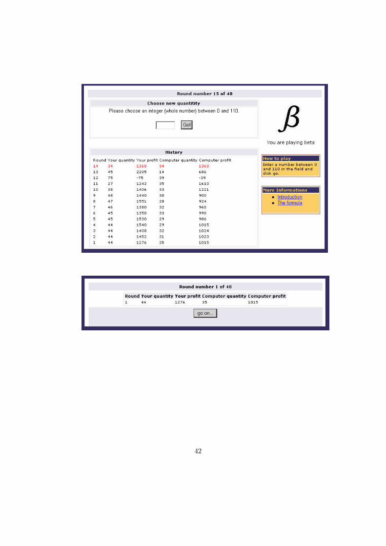
first round. The computer displayed a new window with the results for the
current round including the number of the round, the subject’s quantity, the
subject’s profit, the computer’s quantity as well as the computer’s profit (see
Appendix B for screenshots). A subject had to acknowledge this information
before moving on to the following round. Upon acknowledgment, a new page
appeared with an input field for the new quantity. This page also showed a
table with the history of previous round(s)’s quantities and profits for both
players.
After round 40, subjects were asked to fill in a brief questionnaire (see
Appendix) with information on gender, occupation, country of origin, for-
mal training in game theory or economic theory, previous participation in
online experiments, and the free format question “Please explain in a few
words how you made your decisions”. It was possible to skip this ques-
tionnaire. The highscore was displayed on the following page. This table
contained a ranking among all previous subjects, separately for subjects who
were matched against the same computer type and for all subjects. It also
contained the computer’s highscore.
In both the net and the lab setting, subjects were able to see the entire
history from the previous rounds. In an additional internet setting called
“no history” (noh) we restricted this information to that from the previous
12
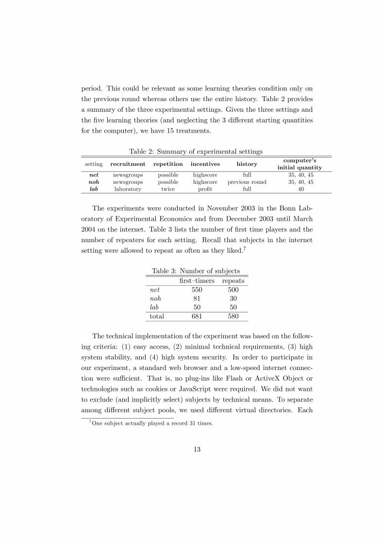
period. This could be relevant as some learning theories condition only on
the previous round whereas others use the entire history. Table 2 provides
a summary of the three experimental settings. Given the three settings and
the five learning theories (and neglecting the 3 different starting quantities
Note: Average quantities over all 40 rounds and all subjects in a given treatment.The Cournot-Nash equilibrium quantity is 36. Standard errors of means in
parentheses.
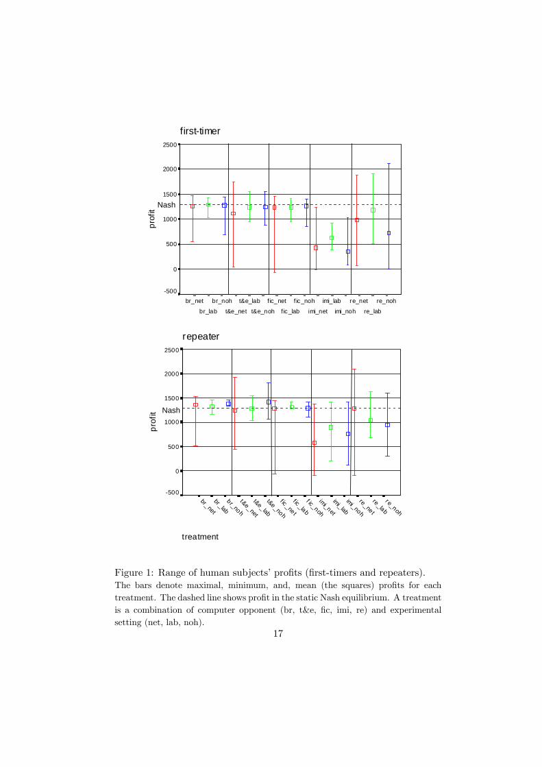
report those measures separately for each of our treatments, i.e. for each
combination of computer type (br, t&e, fic, imi, and re) and setting (net,
lab, noh). The dotted line indicates the profit per round in the Cournot
Nash equilibrium.
First time players who are matched with a computer types br, t&e, or
fic achieve on average slightly less than the Nash equilibrium profit. The
ranges in profits are larger in the internet treatments than in the lab but
roughly comparable across the three computer types. Drastically different,
however, are profits of subjects who were matched against the computer
types imi and re. On average profits against imi were less than half the
profits against the first three computer types. Even the very best subjects
do not reach the Nash equilibrium profit, despite the bias in the noise of
this computer type (see Footnote 4). Profits against computer type re are
15
also substantially lower than against br, t&e, or fic but they are higher than
against imi.8 The range of profits is highest against this type of computer.
Some subjects achieve very high profits that exceed the Stackelberg leader
or collusive profit (of 1458).
Average profits of repeaters are generally higher than those of first time
players. The improvements, however, seem to be more pronounced for the
internet treatments where subjects could repeat several times and had the
choice of computer opponent. While subjects improve somewhat against
computer type imi, average payoffs are still by far the lowest of all computer
types. Against br and fic, subjects on average do better than the Nash
equilibrium profit. The very best subjects played against t&e and re on the
internet.
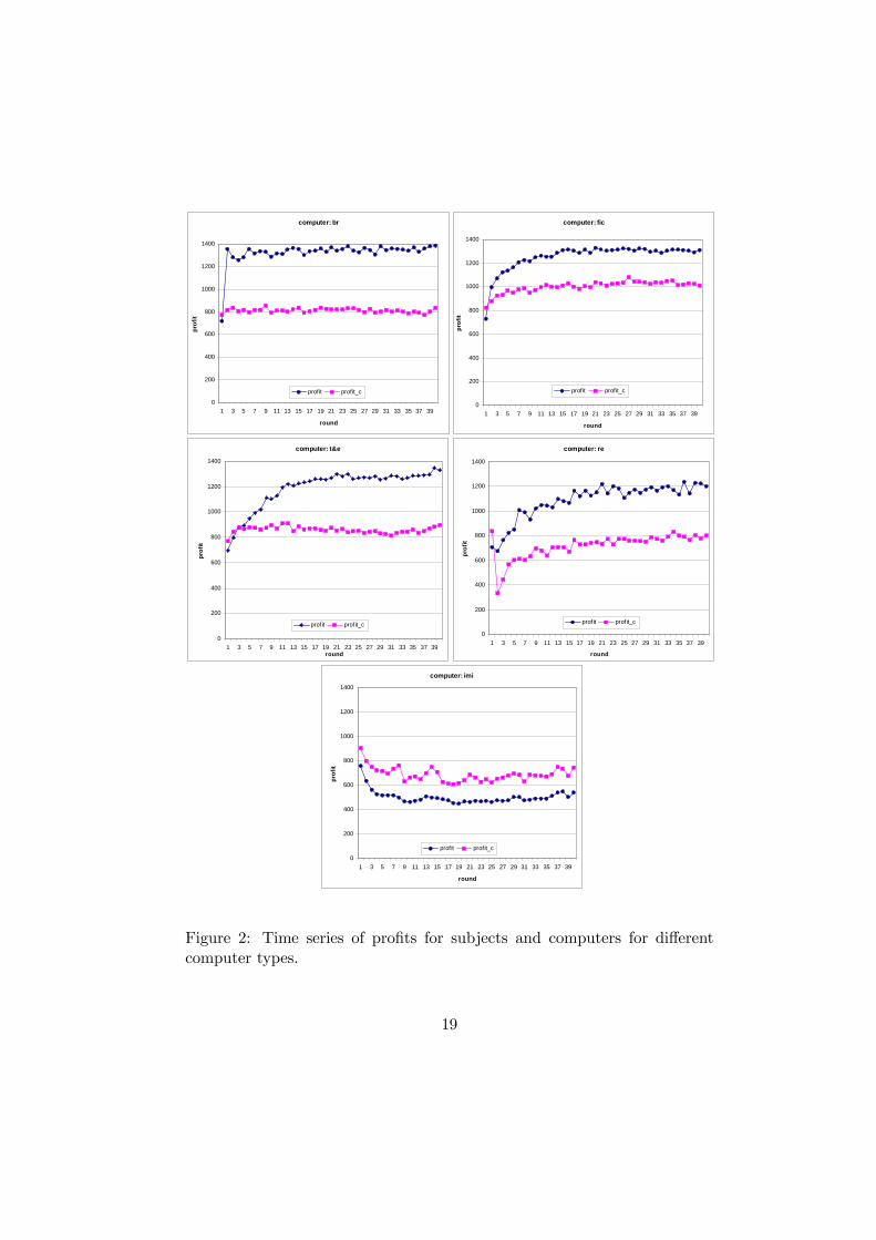
It is also quite instructive to consider average profits over time. Figure
2 shows profits (averaged over settings net, lab, noh and all subjects) of
subjects and computers for all 40 periods. Subjects playing against type
br almost immediately gain a substantive edge over the computer and keep
their profits more or less constant somewhere between the Stackelberg leader
profit and the Nash equilibrium profit. The final result against type fic is
similar but convergence is much more gradual. This shows a considerable
amount of foresight on the side of our subjects. When playing against fic
(in contrast to br), subjects must be more patient and forward looking to
“teach” the computer into a Stackelberg follower positions. The fictitious
play computer is also the most successful among the computer types as it
stabilizes at a profit of above 1000. The time series against types t&e and
re look similar, although against the latter subjects do not even manage to
achieve the Nash equilibrium profit on average.9
Computer type imi yields a totally different picture. In contrast to all
others, payoffs against imi decrease over time, both for subjects and for com-
8For first-time players, profits against re are lower than against br, fic, and t&e accord-ing to two—sided MWU tests at p < 0.01. For repeaters only the first difference remainssignificant at p = 0.02. For both, first-timers and repeaters, profits against re are higherthan against imi at p < 0.001.
9The dip of the computers’ profits in round 2 is due to the high relative weight of the(uniformly distributed) initial weights in early rounds, while the computer quantity inround 1 is not chosen by the learning theory, but set to 35, 40 or 45.
16
first-timer
treatment
re_noh
re_lab
re_net
imi_noh
imi_lab
imi_net
f ic_noh
fic_lab
fic_net
t&e_noh
t&e_lab
t&e_net
br_noh
br_lab
br_net
prof
it2500
2000
1500
1000
500
0
-500
repeater
treatment
re_noh
re_lab
re_net
imi_noh
imi_lab
imi_net
f ic_noh
f ic _lab
f ic _net
t&e_noh
t&e_lab
t&e_net
br_noh
br_labbr_net
prof
it
2500
2000
1500
1000
500
0
-500
Nash
Nash
Figure 1: Range of human subjects’ profits (first-timers and repeaters).The bars denote maximal, minimum, and, mean (the squares) profits for eachtreatment. The dashed line shows profit in the static Nash equilibrium. A treatmentis a combination of computer opponent (br, t&e, fic, imi, re) and experimentalsetting (net, lab, noh).
17
puters. Furthermore, it is the only computer type where subjects’ payoffs
are lower than those of computers. We say more on this below.
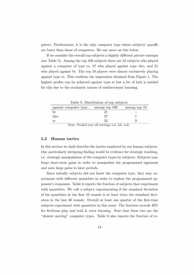
If we consider the overall top subjects a slightly different picture emerges
(see Table 5). Among the top 100 subjects there are 52 subjects who played
against a computer of type re, 27 who played against type t&e, and 21
who played against br. The top 10 players were almost exclusively playing
against type re. This confirms the impression obtained from Figure 1. The
highest profits can be achieved against type re but a lot of luck is needed
for this due to the stochastic nature of reinforcement learning.
Table 5: Distribution of top subjectsagainst computer type... among top 100 among top 10br 21 −t&e 27 1re 52 9
Note: Pooled over all settings net, lab, noh.
5.2 Human tactics
In this section we shall describe the tactics employed by our human subjects.
One particularly intriguing finding would be evidence for strategic teaching,
i.e. strategic manipulation of the computer types by subjects. Subjects may
forgo short-term gains in order to manipulate the programmed opponent
and earn large gains in later periods.
Since initially subjects did not know the computer type, they may ex-
periment with different quantities in order to explore the programmed op-
ponent’s responses. Table 6 reports the fraction of subjects that experiment
with quantities. We call a subject experimenting if the standard deviation
of his quantities in the first 10 rounds is at least twice the standard devi-
ation in the last 30 rounds. Overall at least one quarter of the first-time
subjects experiment with quantities in this sense. The fraction exceeds 40%
for fictitious play and trail & error learning. Note that these two are the
“slowest moving” computer types. Table 6 also reports the fraction of re-
Once subjects have explored and learned about the computer type, they
may use this information to actively manipulate the computer type. Such
manipulations may take on various forms. Probably the most straightfor-
ward form of manipulation is aimed at achieving Stackelberg leadership
through aggressive play of large quantities. Table 6 also reports the fraction
of subjects with such leadership behavior. We define a subject as displaying
20
leadership behavior if he chooses a quantity of least 50 for at least 36 out of
40 rounds. About 15% of the first-timers display such leadership behavior.
When playing against best response or trial & error learning, this behavior
becomes even more pronounced among repeaters. The increase in leader-
ship behavior is most remarkable when subjects play against br. Indeed,
playing aggressively is a quite successful manipulation of br. Figure 3(a)
shows quantities of the most successful subject playing against br and the
corresponding computer quantities. This subject (ranked overall 57th) chose
55 in all 40 periods.10 The computer quickly adjusted to a neighborhood of
the Stackelberg follower quantity with the remaining movement due to the
noise in the computer’s decision rule.
Interestingly, we did not find much evidence for manipulation aimed at
collusion in the repeated Cournot duopoly. We call a player collusive if he
played in the first 5 rounds a quantity of at most 30. Collusive behavior
is below 3% for first-timers and repeaters across all computer types except
for imitate-the-best, where it increases from 1% for first-timers to 16% for
repeaters. Apparently a fraction of repeaters learned that the computer will
quickly imitate high quantities which diminishes profits. So by setting low
quantities, the computer may imitate only those low quantities. Against
computer types br, fic, and imi, collusion is theoretically impossible. Only
for t&e there are theoretical results (Huck, Normann, and Oechssler, 2004a)
which indicate that collusion could occur. However, as data on individual
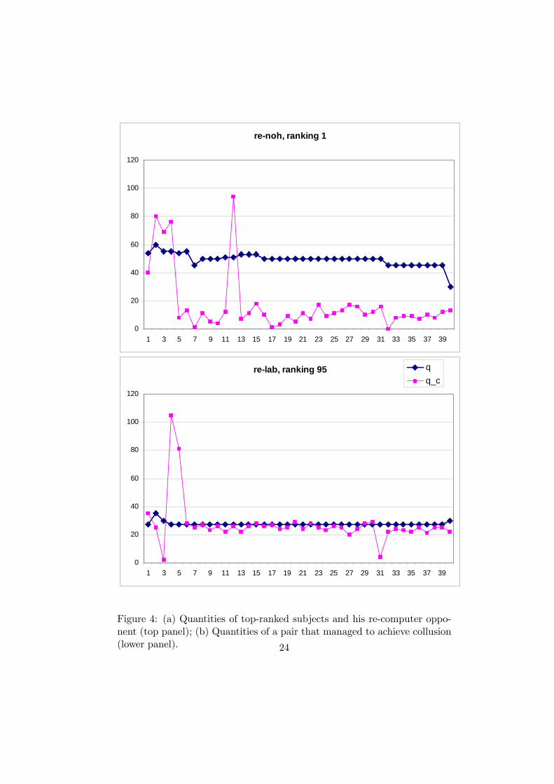
plays reveal, the only successful example of collusion between subject and
computer over a prolonged period occurred against type re (see Figure 4(b)).
Here the computer got locked in at about 27 and the subject consistently
played 27. Of course, the subject could have improved his payoff by deviating
to the best reply to 27 once the computer was locked in sufficiently.
While leadership or collusion may be relatively simple forms of strategic
manipulation, individual data reveal manipulations that can be very sophis-
ticated. We discovered quite interesting, though not very frequent, patterns
that can be seen in the example of Figure 3(b). The subject who played
against best response chose — with only slight variations — the following cycle
10Curiously, none of our subjects chose the exact Stackelberg leader quantity of 54.
21
of 4 quantities: 108, 70, 54, 42, 108, 70, ... Stunningly, this cycle produces
an expected profit per round of 1520, which exceeds the Stackelberg leader
profit.11 By flooding the market with a quantity of 108, the subjects made
sure that the computer left the market in the next period. But instead of
going for the monopoly profit, the subject accumulated intermediate profits
over three periods. This, of course, raises the question, whether a cycle is
optimal and how the optimal cycle looks like. It turns out, that in this game
a cycle of length is four is optimal and, after rounding to integers, the op-
timal cycle is 108, 68, 54, 41, which produces an expected profit of 1522.12
Thus, our subject was within 2 units of the solution for this non—trivial
optimization problem.13
How did the very best subject play? Like all top players, he played
against computer type re. Figure 4(a) reveals that the subject simply got
lucky.14 It was a first-time player in the no-history setting, i.e., a player
with very little information about the game. The reinforcement algorithm
locked in at very low quantities in the range of 10 and the subject roughly
played a best response to that, which resulted in an average profit of 2117.
One benchmark to compare the behavior of our subjects to is the maxi-
mal profit an omniscient, myopic player could achieve against the respective
learning theory. To generate this benchmark, we ran simulations pitting
our 5 computer types against a simulated player who can perfectly forecast
the action his computer opponent is about to take (including the noise) and
plays a best response to that, but disregards the influence of his action on the
future behavior of his opponent. As Figure 5 shows, our repeater subjects
outperform that benchmark against br, re, and t&e. They do worse than the
benchmark against fictitious play but considerably worse only against imi-
tate the best. Given that the myopic best behavior requires a huge amount of
11The only reason the subjects in Figure 3(a) received an even higher payoff was luckdue to favorable noise of the computer algorithm.12See Schipper (2006) for a proof of this claim.13The subject played three times against br and left two comments. The first was “tried
to trick him”, the second “tricked him”.14The description of his strategy was “π mal Daumen”, which roughly translates to
Figure 3: (a) Quantities of subject ranked number 57 and of the br-computeropponent (top panel); (b) Quantities of subject ranked number 61 and ofthe br-computer opponent (lower panel)
Figure 4: (a) Quantities of top-ranked subjects and his re-computer oppo-nent (top panel); (b) Quantities of a pair that managed to achieve collusion(lower panel). 24
knowledge about the opponent, which our subjects can not possibly possess,
since each learning theory incorporates a random element, the only way for
subjects to match or outperform the best myopic benchmark is by playing
better than myopic: By influencing future play of the learning theories.
5.3 Can (myopic) learning theories describe subjects’ behav-ior?
Are the myopic learning theories useful in describing subjects’ behavior? In
this section we analyze whether the same learning theories that were used to
program the computers can be used to organize the behavior of their human
opponents. We shall do so by calculating for each round (except rounds 1
and 2) the quantity q̂ti , which is predicted by the respective theory (without
noise) for round t given the actual history of play up to that moment (i.e.
given all actual decisions of the human subject and the computer opponent
from round 1 through t − 1).15 The predicted action is then compared
to the actually chosen quantity in that round, qti .16 The mean squared
deviation (MSD), (q̂ti − qti)2, is then calculated for each theory by averaging
over all periods t = 3, ..., 40, all subjects, and all treatments. We also
calculate MSDs for the predictions of constant play of the Stackelberg leader
quantity, for constant play of the Cournot Nash equilibrium quantity, for
constant play of the collusive quantity, and for simply repeating the quantity
decision from the previous round (“same”). Finally, as a benchmark we
calculate the MSD that would result from random choice generated by an
i.i.d. uniform distribution on [0,109] (“random”). Figures 6 and 7 show
the resulting average MSD for the settings net and lab separately. Both
figures demonstrate that all predictions perform substantially better than
random choice. Reinforcement has the lowest MSD, followed by trial&error,
same, and imitation.17 Not surprisingly, collusion is very far off the mark.
15Note that we do not replace human play by the theoretical predictions for past rounds.When calculating the history, only actually chosen actions enter.16 In the case of reinforcement learning we take q̂ti to be the expected quantity given the
distribution of propensities.17The performance of “same” may look surprising. But note that subjects who con-
sistently play Stackelberg leader or Cournot would be classified as “same”. Furthermore,in many cases imitation and “same” predict the same action (when the subject has the
25
0 200 400 600 800 1000 1200 1400 1600
fic simulation
fic first time
fic repeat
br simulation
br first time
br repeat
re simulation
re first time
re repeat
imi simulation
imi first time
imi repeat
t&e simulation
t&e first time
t&e repeat
Figure 5: Average profits per round of simulated omniscient, myopicplayer (light grey) vs. actual profits of repeaters (black) and first-time subjects (dark grey) when matched against the different computertypes (e.g. re repeat is the average profit of repeaters against computerre, re simulation is average profit of the omniscient player against re.Note: The omniscient player can perfectly predict the computer’s action (includingnoise).
26
A similar picture emerges for both experimental settings except that MSDs
in the lab are generally much lower than in the internet setting. It seems
that subjects in the lab are better described by our theories.
A slightly different ranking of learning theories is obtained when we con-
sider the theory that best describes a subject’s play (measured by minimum
MSD for all decisions of a given subject in periods 2 through 40). Figure
8 lists the number of subjects’ plays that are best described by the various
theories. Here imitation is most frequently the best fitting theory. Overall,
we see that the myopic learning theories do have some descriptive power.
Yet, given the observed tendency of subjects towards strategic teaching, we
should not be surprised that the fit is all but perfect.
5.4 A comparison with human vs. human data
It should be interesting to compare the behavior of our subjects to that of
subjects in a “normal” experiment where subjects play against other humans
subjects instead of computers. For this purpose we look at the duopoly
treatment of Huck, Normann, and Oechssler (2004b), which has a fairly
similar design as the current experiment.18 A striking difference in results
appears when we compare the average quantities of human subjects. While
in Huck, Normann, and Oechssler (2004b) the average quantity of (human)
subjects is about 9% below the Nash equilibrium quantity, it is more than
33% above the Nash quantity for human subjects in the current experiment
(more than 17% above Nash in lab). That is, when subjects know that their
opponents are also human subjects, they behave slightly collusive. When
they know that they play against computers, they play substantially more
aggressively.
As in the previous subsection we can calculate the MSD for how well
the studied learning theories describe humans’ behavior. Figure 9 shows the
higher profit).18The main differences in the design are that Huck, Normann, and Oechssler (2004b)
use a demand function with p = 100−qi− q−i and a finer grid of strategies. Furthermore,their experiment lasted for only 25 periods. All other design features were essentially thesame.
27
reinforcement
trial&error
sameimitation
Stackelberg leader
fictitious play
best reply
Cournot
collusion
Random
theory
0
200
400
600
800
1,000
1,200
1,400
Ave
rage
MSD
Figure 6: Average MSD for various theoretical predictions, setting netNote: Average is taken over all periods, all subjects, and all treatments.
reinforcement
trial&error
sameimitation
Stackelberg leader
fictitious play
best reply
Cournot
collusion
Random
theory
0
200
400
600
800
1,000
1,200
1,400
Ave
rage
MSD
Figure 7: Average MSD for various theoretical predictions, setting labNote: Average is taken over all periods, all subjects, and all treatments.
28
050
100150200250300350400450500
imita
tion
sam
e
rein
forc
emen
t
Sta
ckel
berg
lead
er
trial
&err
or
Cou
rnot
Fict
itiou
sP
lay
best
resp
onse
Col
lusi
on
Figure 8: Number of plays best described by the various theoretical predic-tions, all settingsNote: A theory is said to best describe a subject’s play if it minimizes MSD overperiods 3-40 of that play.
average MSD for each of the learning theories best response, fictitious play,
imitation, reinforcement learning, and trial & error, for our human vs. com-
puter experiment and Huck et al.’s (2004b) human vs. human experiment,
respectively. Note that the levels of the MSD for the two experiments are
not perfectly comparable since the demand functions differ slightly. Never-
theless, it is striking how much lower the average MSD are for the human
vs. human experiment. In any case, the ranking of the different learning
theories in terms of MSD is informative, and this ranking is almost exactly
reversed: those theories that describe the human behavior worst in our ex-
periment, namely best response and fictitious play, turn out to be those
that describe human behavior best in the context of a human vs. human
situation.
When we look at the average MSD for all 5 learning theories, we see
29
human vs. computer
0
50
100
150
200
250
300
350
400
450
best response fictitious play imitation reinforcement trial & error
Theory
Ave
rage
MS
D
human vs. human
0
50
100
150
200
250
300
350
400
450
best response fictitious play imitation reinforcement trial & error
Theory
Ave
rage
MSD
Figure 9: Average MSD of different learning theories in human vs. com-puters experiment (top panel), and in human vs human experiment (lowerpanel).
30
that descriptive power of those theories becomes better over time. Figure
10 shows the development of average MSD for all theories, separately for
our human vs. computer experiment and Huck et al.’s (2004b) human vs.
human experiment. While there is improvement for both experiments, the
improvement in the human vs. human case is much stronger.
What could account for this? Both, best response and fictitious play
work well when describing play near a Cournot equilibrium. Looking at
Table 4, we see that subjects are more likely to play quantities close to the
Cournot equilibrium when playing against other humans, and consequently
are better described by fictitious play and best response. But why does
this not apply when playing against a computer? It seems that strategic
teaching is more pronounced when playing against a computer. Strategic
teaching in our context usually consists of playing higher quantities to in-
duce the computer to react with lower quantities in future rounds. Since
such forward-looking behavior is not predicted by any of the five (adaptive)
learning theories, average MSDs remain relatively high in the human vs.
computer experiment.
Reasons for the subjects to use less strategic teaching against other hu-
mans could include fairness considerations (the Cournot outcome is “fairer”
than the Stackelberg outcome) and the anticipation of negative reciprocal re-
actions. Alternatively, subjects may believe that real subjects are harder to
fool (or more stubborn) than a simple computer program and are therefore
less susceptible to strategic teaching. Of course, there is no good reason for
supposing that computers could not be programmed to mimic “emotional”
reactions of humans like reciprocity, revenge, or, indeed, rage. But probably
our dominant perception of computers is one of rationally acting machines
without emotions.
5.5 Learning theories and economic value
We define the economic value of a given learning theory as the improvement
in a subject’s profit generated by substituting the learning theory’s recom-
mendation for the actual choice of the subject (compare Camerer and Ho,
2001), where the learning theory’s choice is based on the real history of play
Figure 10: Average MSD of all 5 learning theories over time in humanvs. computer experiment (top panel) and in human vs. human experiment(lower panel).
32
up to that round. Note that this is of course a very myopic point of view:
only improvements in payoffs for the current period are counted whereas
possible long—term gains are ignored.
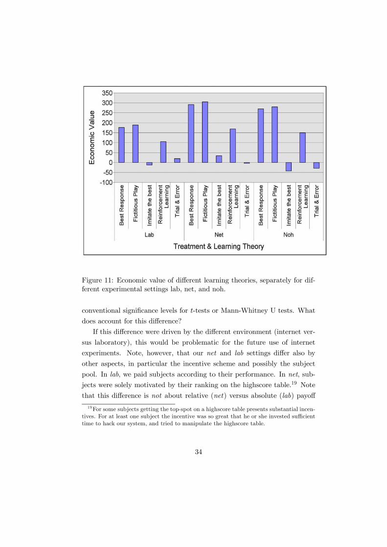
Figure 11 shows the average economic value that the five different learn-
ing theories would have generated for our subjects, separately for the three
experimental settings lab, net, and noh, and the five learning theories. While
the economic value of “imitate the best” is rather low and that of “trial &
error” even negative, there are substantial potential gains from switching to
best response, fictitious play, or reinforcement learning, considering that the
average profit per round was about 1112. Figure 11 shows that the ranking
of the learning theories in terms of economic value are very similar across
experimental settings, but the levels are lower in lab. Just as our subjects
in lab are better described by the learning theories, the additional value of
having those learning theories’ advice is reduced.
As pointed out above, it should not come as a surprise that the economic
values are so high despite the fact that subjects actually achieved much
higher profits than computers. Since economic value does not capture the
long-term effects of a strategy, it does not capture strategic teaching. As we
saw in Section 5.2, quite a number of our subjects were successfully trying
to exploit the learning theories’ algorithms by deliberately foregoing profits
in the current round to induce the computer opponent to play in a way
that enables the human to gain larger profits in future rounds. Thus, high
economic value may just be a sign that a subject is deliberately deviating
from the myopic optimum to maximize long-term profits.
5.6 Experimenting on the internet - does it make a differ-ence?
Looking at Table 4 it is apparent that subjects’ average quantities on the net
seem to be substantially higher than in the lab. In fact, when we aggregate
the mean quantities shown in Table 4 over computer types, we get average
quantities of 48.68 in net and 42.30 in lab. This difference is significant at all
33
Figure 11: Economic value of different learning theories, separately for dif-ferent experimental settings lab, net, and noh.
conventional significance levels for t-tests or Mann-Whitney U tests. What
does account for this difference?
If this difference were driven by the different environment (internet ver-
sus laboratory), this would be problematic for the future use of internet
experiments. Note, however, that our net and lab settings differ also by
other aspects, in particular the incentive scheme and possibly the subject
pool. In lab, we paid subjects according to their performance. In net, sub-
jects were solely motivated by their ranking on the highscore table.19 Note
that this difference is not about relative (net) versus absolute (lab) payoff
19For some subjects getting the top-spot on a highscore table presents substantial incen-tives. For at least one subject the incentive was so great that he or she invested sufficienttime to hack our system, and tried to manipulate the highscore table.
34
maximization. A subjects needs to maximize his absolute payoff in order to
achieve a large highscore.
To sort those things out, we have conducted experiments with two addi-
tional settings. The two new settings are designed to bridge the gap between
the lab and net settings. The setting “lab-f” is just like the lab setting ex-
cept that subjects received a fixed payment of 10 Euros as soon as they
entered the lab.20 Setting “lab-np” is like lab except that subjects received
no payment at all. Thus, in both new settings, a good placement on the
highscore table was the only motivation for subjects. The only difference
between lab-np and net was the environment, that is, the laboratory versus
subjects’ homes or offices. To summarize, the new and old settings can be
ordered as follows.
labincentive vs. fixed pay←→
(p<.001)lab-f
fixed pay vs. no pay←→(p=0.228)
lab-np lab vs. home←→(p=0.224)
net
(5)
The experiments for setting lab-f were conducted in October 2004 in the
Bonn Laboratory of Experimental Economics. There were 50 subjects who
each played twice against the same computer type, just like in setting lab.
Subjects for setting lab-np were volunteers who took part in an introduc-
tion for freshmen during which they visited the laboratory. There were 55
volunteers of which 5 played a second time.
Each of the arrows in (5) could account for the difference in quantities
between lab and net. Table 7 shows mean quantities for the different setting
for first-time players and all subjects, separately.
Table 7 shows clearly that there is a significant difference only for the
first of those arrows, i.e. between lab and lab-f. There are no significant
differences at any conventional level between lab-f, lab-np, and net.21 We
conclude that the difference between lab and net is primarily driven by the
lack of monetary incentives in net and not by the environment of the decision
20 In principle, subjects could have left the lab after receiving the 10 Euros but no onedid.21The p—values shown in equation (5) refer to all subjects’ mean quantities using a
Mann-Whitney U test, treating each subject as one observation. For first-timers the p-values are similar.
35
Table 7: Mean quantities
settingfirst-timers’
mean quantitiesall subjects’
mean quantitieslab 43.14 42.30lab-f 48.21 47.65lab-np 48.85 48.52net 48.69 48.68
Note: Average quantities over all 40 rounds.
maker.22
For future internet experiments we would thus suggest the use of sig-
nificant financial incentives. However, even if we find significantly higher
quantities in net, the main results of the paper holds for both settings net
and lab. Namely, quantities of subjects are much higher than quantities of
the computer against all computer types except imi (see Table 4). They are
also substantially higher than the Nash equilibrium quantity. This indicates
that a large part of our subjects were not just myopic optimizers but instead
tried to actively influence their opponents.
6 Conclusion
In this experiment we let subjects play against computers which were pro-
grammed to follow one of a set of popular learning theories. The aim was
to find out whether subjects were able to exploit those learning algorithms.
The bulk of the (boundedly rational) learning theories that have been stud-
ied in the literature (see Fudenberg and Levine, 1998, for a good overview)
are myopic in nature. Probably the most fundamental insight from our ex-
periment is that we need to advance to theories that incorporate at least a
limited amount of foresight. Many of our subjects were quite able to exploit
the simple myopic learning algorithms. Strategic teaching is an important
phenomenon that needs to be accounted for in the future development of
22For this conclusion to hold, we make the (probably not too implausible) assumptionthat the marginal effect of providing monetary incentives is the same in the laboratoryand on the internet.
36
theory. Yet, a word of caution is in order. A comparison with human vs.
human data reveals that myopic learning theories are much better able to
explain behavior than in our human vs. computer experiment. Why this is
so, remains an interesting question for future work.
Our experiment also provides some methodological lessons with respect
to internet experiments. Although we found significant differences between
our internet and our laboratory setting, we could account for those differ-
ences through the different incentive schemes. Internet experiments are fine,
as long as subjects have proper monetary incentives.
37
Appendix
A Instructions
A.1 Introduction Page Internet
Welcome to our experiment!
Please take your time to read this short introduction. The experiment lasts for
40 rounds. At the end, there is a high score showing the rankings of all participants.
You represent a firm which produces and sells a certain product. There is one
other firm that produces and sells the same product. You must decide how much
to produce in each round. The capacity of your factory allows you to produce
between 0 and 110 units each round. Production costs are 1 per unit. The price
you obtain for each sold unit may vary between 0 and 109 and is determined as
follows. The higher the combined output of you and the other firm, the lower the
price. To be precise, the price falls by 1 for each additional unit supplied. The
profit you make per unit equals the price minus production cost of 1. Note that
you make a loss if the price is 0. Your profit in a given round equals the profit per
unit times your output, i.e. profit = (price 1) * Your output. Please look for an
example here. At the beginning of each round, all prior decisions and profits are
shown. The other firm is always played by a computer program. The computer
uses a fixed algorithm to calculate its output which may depend on a number of
things but it cannot observe your output from the current round before making its
decision. Your profits from all 40 rounds will be added up to calculate your high
score. There is an overall high score and a separate one for each type of computer.
Please do not use the browser buttons (back, forward) during the game, and do not
click twice on the go button, it may take a short while.
Choose new quantity
Please choose an integer (whole number) between 0 and 110.
A.2 Introduction Page lab
Welcome to our experiment!
Please take your time to read this short introduction. The experiment lasts
for 40 rounds. Money in the experiment is denominated in Taler (T). At the end,
38
exchange your earnings into Euro at a rate of 9.000 Taler = 1 Euro. You represent
a firm which produces and sells a certain product. There is one other firm that
produces and sells the same product. You must decide how much to produce in
each round. The capacity of your factory allows you to produce between 0 and 110
units each round. Production cost are 1T per unit. The price you obtain for each
sold unit may vary between 0 T and 109 T and is determined as follows. The higher
the combined output of you and the other firm, the lower the price. To be precise,
the price falls by 1T for each additional unit supplied. The profit you make per unit
equals the price minus production cost of 1T. Note that you make a loss if the price
is 0. Your profit in a given round equals the profit per unit times your output, i.e.
profit = (price 1) * Your output. Please look for an example here. At the beginning
of each round, all prior decisions and profits are shown. The other firm is always
played by a computer program. The computer uses a fixed algorithm to calculate
its output which may depend on a number of things but it cannot observe your
output from the current round before making its decision. Your profits from all 40
rounds will be added up to calculate your total earnings. Please do not use the
browser buttons (back, forward) during the game, and do not click twice on the go
button, it may take a short while.
Choose new quantity
Please choose an integer (whole number) between 0 and 110.
A.3 Example Page
The Formula
The profit in each round is calculated according to the following formula:
Profit = (Price 1) * Your Output
The price, in turn, is calculated as follows.
Price = 109 Combined Output
That is, if either you or the computer raises the output by 1, the price falls
by 1 for both of you. (but note that the price cannot become negative). And the
combined output is simply:
Combined Output = Your Output + Computers Output
Example:
39
Lets say your output is 20, and the computers output is 40. Hence, combined
output is 60 and the price would be 49 (= 109 - 60). Your profit would be (49 1)*20
= 960. The computers profit would be (49 - 1)*40 = 1920. Now assume you raise
your output to 30, while the computer stays at 40. The new price would be 39 ( =
109-40-30). Your profit would be (39 - 1)*30 = 1140. The computers profit would
be (39 - 1)*40 = 1520.
To continue, please close this window.
B Screenshots
40
41
42
References
[1] Alós—Ferrer, C. (2004). Cournot vs. Walras in dynamic oligopolies with
memory, International Journal of Industrial Organization, 22, 193-217.
[2] Apesteguia, J., Huck, S. and Oechssler, J. (2006). Imitation - Theory
and experimental evidence, forthcoming, Journal of Economic Theory.
[3] Brown, G.W. (1951). Iterative solutions of games by fictitious play, in:
Koopmans, T.C. (ed.), Activity analysis of production and allocation,
John Wiley.
[4] Camerer, C., and Ho, T.H. (2001). Strategic learning and teaching in
games, in: S. Hoch and H. Kunreuther (eds.) Wharton on decision
making, New York: Wiley.
[5] Camerer, C., Ho, T.H. and Chong, J.K. (2002). Sophisticated
experience-weighted attraction Learning and strategic teaching in re-
peated games, Journal of Economic Theory, 104, 137-188.
[6] Coricelli, G. (2005). Strategic interaction in iterated zero-sum games,
Homo Oeconomicus, forthcoming.
[7] Cournot, A. (1838). Researches into the mathematical principles of the
theory of wealth, transl. by N. T. Bacon, MacMillan Company, New
York, 1927.
[8] Drehmann, M., Oechssler, J. and Roider, A. (2005). Herding and con-
trarian behavior in financial markets, American Economic Review,
95(5), 1403-1426..
[9] Ellison, G. (1997). Learning from personal experience: One rational
guy and the justification of myopia, Games and Economic Behavior,
19, 180-210.
[10] Erev, I. and Roth, A. (1998). Predicting how people play games: Rein-
forcement learning in experimental games with unique, mixed strategy
equilibria, American Economic Review, 88, 848-881.
43
[11] Fox, J. (1972). The learning of strategies in a simple, two-person zero-
sum game without saddlepoint, Behavioral Science, 17, 300-308.
[12] Fudenberg, D., and Levine, D. (1998). The theory of learning in games,
Cambridge: MIT Press.
[13] Houser, D. and Kurzban, R. (2002). Revisiting kindness and confusion
in public goods experiments, American Economic Review, 94, 1062-
1069.
[14] Huck, S., Normann, H.T., and Oechssler, J. (1999). Learning in Cournot
oligopoly: An experiment, Economic Journal, 109, C80-C95.
[15] Huck, S., Normann, H.T., and Oechssler, J. (2004a). Through trial &
error to collusion, International Economic Review, 45, 205-224.
[16] Huck, S., Normann, H.T., and Oechssler, J. (2004b). Two are few and
four are many: Number effects in experimental oligopoly, Journal of
Economic Behavior and Organization, 53, 435-446.
[17] Ianni, A. (2002). Reinforcement learning and the power law of practice:
Some analytical results, University of Southampton.
[18] Kirchkamp, O. and Nagel, R. (2007). Naive learning and cooperation
in network experiments, Games and Economic Behavior, 58, 269-292.
[19] Laslier, J.-F., Topol, R. and Walliser, B. (2001). A behavioral learning
process in games, Games and Economic Behavior, 37, 340-366.
[20] Lieberman, B. (1962). Experimental studies of conflict in some two-
person and three-person games, in: Criswell, J. H., Solomon, H. and
Suppes, P. (eds.), Mathematical methods in small group processes,
Stanford University Press, 203-220.
[21] Matros, A. (2004). Simple Rules and Evolutionary Selection, University
of Pittsburgh.
44
[22] McCabe, K., Houser, D., Ryan, L., Smith, V. and Trouard, T. (2001).
A functional imaging study of cooperation in two-person reciprocal ex-
change, Proceedings of the National Academy of Sciences, 98, 11832-
11835.
[23] Messick, D.M. (1967). Interdependent decision strategies in zero-sum
games: A computer controlled study, Behavioral Science, 12, 33-48.
[24] Monderer, D. and Shapley, L. (1996). Potential games, Games and Eco-
nomic Behavior, 14, 124-143.
[25] Offerman, T., Potters, J., and Sonnemans, J. (2002). Imitation and
belief learning in an oligopoly experiment, Review of Economic Studies,
69, 973-997.
[26] Robinson, J. (1951). An iterative method of solving games, Annals of
Mathematics, 54, 296-301.
[27] Roth, A. and Erev, I. (1995). Learning in extensive form games: Ex-
perimental data and simple dynamic models in the intermediate term,
Games and Economic Behavior 8, 164-212
[28] Roth, A. and Schoumaker, F. (1983). Expectations and reputations in
bargaining: An experimental study, American Economic Review, 73,
362-372.
[29] Sarin, R. and Vahid, F. (2004). Strategic similarity and coordination,
Economic Journal, 114, 506-527.
[30] Schipper, B.C. (2004), Imitators and optimizers in Cournot oligopoly,
University of California, Davis.
[31] Schipper, B.C. (2006), Strategic Control of Myopic Best Reply in Re-
peated Games, University of California, Davis.
[32] Shachat, J. and Swarthout, J. T. (2002). Learning about learning in
games through experimental control of strategic independence, Univer-
sity of Arizona.
45
[33] Thorndike, E.L. (1898). Animal intelligence: An experimental study of
associative processes of animals, Psychological Monographs, 2 (8).
[34] Vega—Redondo, F. (1997). The evolution of Walrasian behavior, Econo-
metrica, 65, 375-384.
[35] Walker, J., Smith, V.L. and Cox, J.C. (1987). Bidding behavior in first