Page 1
v
RAILROAD TIE LATERAL RESISTANCE ON OPEN-DECK PLATE GIRDER
BRIDGES
John T. Gergel
Thesis submitted to the faculty of the Virginia Polytechnic Institute and State
University in partial fulfillment of the requirements for the degree of
MASTER OF SCIENCE
In
CIVIL ENGINEERING
Matthew H. Hebdon, Chair
Matthew R. Eatherton
Ioannis Koutromanos
December 12, 2019
Blacksburg, Virginia
Keywords: railroad bridges, tie fasteners, lateral resistance
Page 2
RAILROAD TIE LATERAL RESISTANCE ON OPEN-DECK PLATE GIRDER
BRIDGES
ABSTRACT
John Gergel
On open-deck railroad bridges, the crossties (sleepers) are directly supported by the bridge
superstructure and anchored with deck tie fasteners such as hook bolts. These fasteners provide lateral
resistance for the bridge ties. Currently there are no provisions to assist in the calculation of lateral
resistance provided by railroad ties on open-deck bridges, and as a result there are no specific
requirements for the spacing of deck tie fasteners. This has led to different design practices specific to
each railroad, and inconsistent fastener spacing in existing railroad bridges.
A research plan was conducted to experimentally quantify the lateral resistance of timber crossties on
open-deck plate girder bridges using different wood species and types of fasteners. Experimental tests
were conducted on five different species of timber crossties (beech, sycamore, southern pine, Douglas-fir,
and oak) with three different types of fasteners (square body hooks bolt, forged hook bolts, and Quick-Set
Anchors). A structural test setup simulated one half of an open-deck bridge with a smooth-top steel plate
girder, and hydraulic actuators to apply both vertical and horizontal load to a railroad tie specimen. The
three main contributions to lateral resistance on open-deck bridges were identified as friction resistance
between tie and girder due to vertical load from a truck axle, resistance from the fastener, and resistance
from dapped ties bearing against the girder flange. Initial testing isolated each component of lateral
resistance to determine the friction coefficient between tie and girder as well as resistance from just the
fastener itself. Additional testing combined both vertical load and fastener to determine whether or not the
overall resistance is simply the sum of the friction and fastener resistance. Results indicated that friction
resistance varies based on the magnitude of vertical axle load, species of wood, and creosote retention in
the tie, while fastener resistance varies based on type of fastener and lateral displacement of the tie. An
approximation of the lateral resistance as a function of lateral displacement was established depending on
Page 3
the vertical load, type of hook bolt, and coefficient of friction between tie and girder. The approximation
was used in a structural analysis, which modelled a section of railroad track as a beam supported by non-
linear springs spaced at discrete distance. Based on anticipated lateral loads, the analysis was used to
determine a preliminary chart for a safe and economical fastener spacing for a railroad track based on
type of hook bolt, creosote retention, tie species, and curvature of bridge.
Page 4
RAILROAD TIE LATERAL RESISTANCE ON OPEN-DECK PLATE GIRDER
BRIDGES
GENERAL AUDIENCE ABSTRACT
John Gergel
On open-deck railroad bridges, the crossties are directly supported by the steel bridge girders and
connected to the girders with fasteners as hook bolts. These fasteners provide lateral resistance for the
bridge ties. Currently there are no provisions to assist in the calculation of lateral resistance provided by
railroad ties on open-deck bridges, and as a result there are no specific requirements for the spacing of
deck tie fasteners. This has led to different design practices specific to each railroad, and inconsistent
fastener spacing in existing railroad bridges.
A research plan was conducted to experimentally quantify the lateral resistance of timber crossties on
open-deck plate girder bridges using different wood species and types of fasteners. Experimental tests
were conducted on five different species of timber crossties (beech, sycamore, southern pine, Douglas-fir,
and oak) with three different types of fasteners (square body hooks bolt, forged hook bolts, and Quick-Set
Anchors). A structural test setup simulated one half of an open-deck bridge with a smooth-top steel plate
girder, and hydraulic actuators to apply both vertical and horizontal load to a railroad tie specimen. The
three main contributions to lateral resistance on open-deck bridges were identified as friction resistance
between tie and girder due to vertical load from a truck axle, resistance from the fastener, and resistance
from dapped ties bearing against the girder flange. Initial testing isolated each component of lateral
resistance to determine the friction coefficient between tie and girder as well as resistance from just the
fastener itself. Additional testing combined both vertical load and fastener to determine whether or not the
overall resistance is simply the sum of the friction and fastener resistance. Results indicated that friction
resistance varies based on the magnitude of vertical axle load, species of wood, and creosote retention in
the tie, while fastener resistance varies based on type of fastener and lateral displacement of the tie. An
Page 5
v
approximation of the lateral resistance as a function of lateral displacement was established depending on
the vertical load, type of hook bolt, and coefficient of friction between tie and girder. The approximation
was used in a structural analysis, and the analysis was used to determine a preliminary chart for a safe and
economical fastener spacing for a railroad track based on type of hook bolt, creosote retention, tie species,
and curvature of bridge.
Page 6
vi
Table of Contents
ABSTRACT .................................................................................................................................................. ii
GENERAL AUDIENCE ABSTRACT ........................................................................................................ iv
Table of Contents ......................................................................................................................................... vi
List of Figures .............................................................................................................................................. ix
List of Tables ............................................................................................................................................. xiii
ACKNOWLEDGEMENTS ....................................................................................................................... xiv
CHAPTER 1: INTRODUCTION AND BACKGROUND .......................................................................... 1
1.1 Background and Scope .................................................................................................................... 1
1.2 Objectives ........................................................................................................................................ 3
1.3 Overall Approach ............................................................................................................................. 5
1.4 Scope ................................................................................................................................................ 5
1.4.1 Crossties .................................................................................................................................. 7
1.4.2 Species and Treatment ............................................................................................................ 7
1.4.3 Size and Spacing ..................................................................................................................... 8
CHAPTER 2: LITERATURE REVIEW .................................................................................................... 10
2.1 Train Wheel Dynamics ..................................................................................................................... 10
2.1.1 Wheel Hunting ........................................................................................................................... 11
2.2 Rail Loads ......................................................................................................................................... 12
2.2.1 Vertical Dead Loads................................................................................................................... 13
2.2.2 Cooper E80 and Alternative Live Load ..................................................................................... 13
2.2.3 Actual Vertical Train Live Loads .............................................................................................. 14
2.2.4 Centrifugal Force ....................................................................................................................... 17
2.2.5 Research on Centrifugal Wheel-to-Rail Force ........................................................................... 19
2.2.6 Moving Freight Equipment ........................................................................................................ 20
2.2.7 Impact Loading .......................................................................................................................... 21
2.3 Maximum Vehicle Speed on Curves ................................................................................................ 21
2.4 Lateral Load (Net Axle Ratio) .......................................................................................................... 22
2.5 Vertical Tie Reaction ........................................................................................................................ 23
2.5.1 Winkler Base Model .................................................................................................................. 23
2.5.2 Accuracy of Winkler Model ...................................................................................................... 26
Page 7
vii
2.5.3 AREMA, Talbot, and Kerr Equations ........................................................................................ 27
2.6 Track Lateral Resistance ................................................................................................................... 29
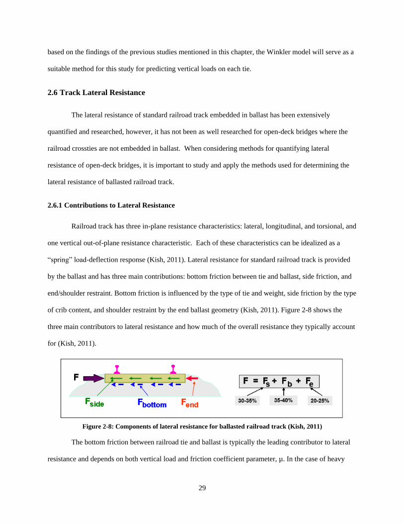
2.6.1 Contributions to Lateral Resistance ........................................................................................... 29
2.6.2 Experimental Methods for Determining Lateral Resistance ...................................................... 30
2.6.3 Predicting Lateral Resistance from STPT .................................................................................. 32
CHAPTER 3: METHODOLOGY .............................................................................................................. 34
3.1 Structural Test Setup ......................................................................................................................... 34
3.2 Friction Testing ................................................................................................................................. 37
3.2.1 Friction Test Methods ................................................................................................................ 37
3.2.2 Wood Species Tested ................................................................................................................. 40
3.2.3 Beech and Sycamore .................................................................................................................. 40
3.2.4 Southern Pine ............................................................................................................................. 41
3.2.5 Oak Species ................................................................................................................................ 43
3.2.6 Douglas-fir Species .................................................................................................................... 45
3.3 Material Testing ................................................................................................................................ 46
3.3.1 Compression Testing ................................................................................................................. 46
3.4 Combined Friction and Fastener Tests .............................................................................................. 48
3.4.1 Combined Square Body Hook Bolt and Forged Hook Bolt Tests ............................................. 48
3.4.2 Combined Friction and Quick-Set Anchor Tests ....................................................................... 52
3.5 Dapped Tie Testing ........................................................................................................................... 54
3.6 Relative Displacement Reading ........................................................................................................ 55
3.7 Cleaning Lateral Load vs. Displacement Data .................................................................................. 58
3.8 Methods of Analysis ......................................................................................................................... 60
3.8.1 Lateral Stiffness Approximations .............................................................................................. 60
3.8.2 Structural Analysis Methods ...................................................................................................... 64
CHAPTER 4: RESULTS AND DISCUSSION .......................................................................................... 70
4.1 Friction Contribution ........................................................................................................................ 70
4.1.1 Friction Test Displacement Corrections .................................................................................... 71
4.1.2 Mixed Hardwood Friction Test Results ..................................................................................... 73
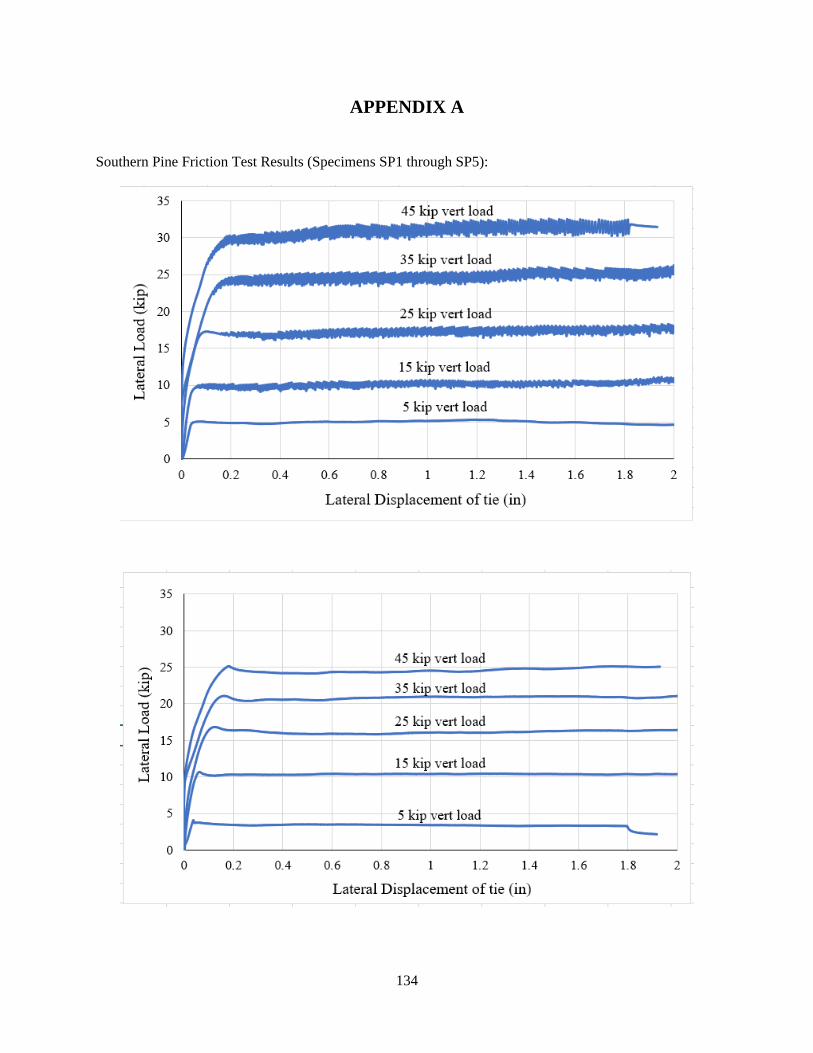
4.1.3 Southern Pine Test Results ........................................................................................................ 74
4.1.4 New Oak Friction Test Results .................................................................................................. 78
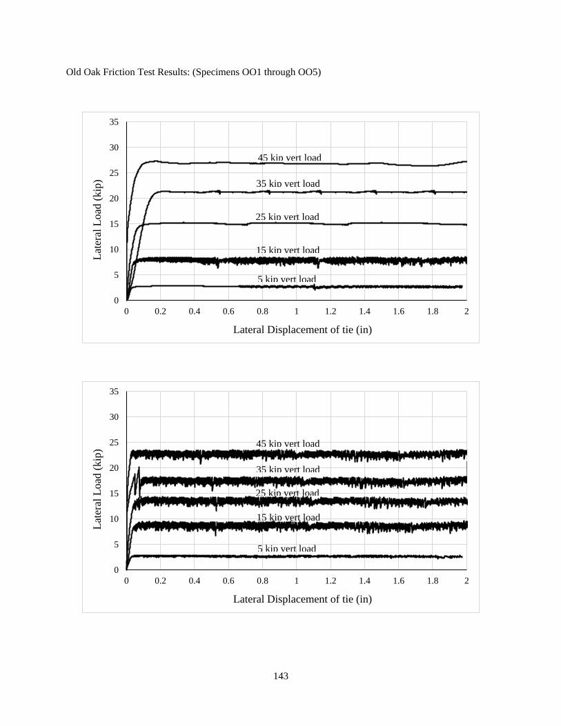
4.1.5 Old Oak Friction Test Results .................................................................................................... 82
4.1.6 Douglas-fir Friction Test Results ............................................................................................... 83
Page 8
viii
4.1.7 Coefficients of Friction .............................................................................................................. 85
4.2 Nut Tightness Dependence on Lateral Resistance ............................................................................ 88
4.3 Combined Friction and Fastener Results .......................................................................................... 91
4.3.1 Combined Testing Displacement Corrections ........................................................................... 91
4.3.2 Combined Friction and Square Body Hook Bolt Results .......................................................... 93
4.3.3 Combined Friction and Forged Hook Bolt Results .................................................................... 98
4.3.4 Combined Friction and Quick-Set Anchor Results .................................................................. 102
4.4 Testing of Dapped Ties ................................................................................................................... 105
4.4.1 Dapped Tie Test Displacement Corrections ............................................................................ 105
4.4.2 Corrected Results of Dapped Tie Tests with no Vertical Load or Fastener ............................. 107
4.4.3 Results of Dapped Tie Tests with Vertical Load and Fastener ................................................ 110
4.5 Lateral Stiffness Approximations ................................................................................................... 111
4.5.1 Friction Only ............................................................................................................................ 111
4.5.2 Friction and Fastener ................................................................................................................ 113
4.5.3 Dapped Ties ............................................................................................................................. 118
4.6 Analysis Results .............................................................................................................................. 120
CHAPTER 5: Conclusions ....................................................................................................................... 129
5.1 Friction Resistance .......................................................................................................................... 129
5.2 Fastener Resistance ......................................................................................................................... 129
5.3 Overall Lateral Resistance .............................................................................................................. 130
REFERENCES ......................................................................................................................................... 131
APPENDIX A ........................................................................................................................................... 134
APPENDIX B ........................................................................................................................................... 151
Page 9
ix
List of Figures
Figure 1-1: Open-deck railway bridge (Unsworth, 2017) ............................................................................. 3
Figure 1-2: Ballasted-deck railway bridge (Unsworth, 2017) ...................................................................... 3
Figure 1-3: Configuration of dapped railroad bridge tie ............................................................................... 4
Figure 1-4: Square body hook bolt (left) and forged hook bolt (right) ......................................................... 6
Figure 1-5: Left - Quick-Set anchor assembly ((Vasudevan, 2018)), Middle - Quick-Set hook bolt, Right -
Quick-Set anchor and bracket installed on ties ((“Patented Quick-Set Hook Bolt System,” 2017)) ............ 7
Figure 1-6: AREMA standard sizes for typical and bridge railroad ties ....................................................... 9
Figure 2-1: Wheelset on straight track (left) vs. wheelset on curved track (right) (Tzanakakis, 2013) ...... 11
Figure 2-2: Cooper E80 live load configuration from AREMA Chapter 15 (AREMA, 2017a) ................. 14
Figure 2-3: Alternate Live Load configuration from AREMA Chapter 15 (AREMA, 2017a) .................. 14
Figure 2-4: Resultant force due to weight of train and centrifugal force (Hook, 2017) ............................. 18
Figure 2-5: Wheel to rail forces assuming a 100-kip axle (Herbert Weinstock, 1980) .............................. 20
Figure 2-6: Beam on an elastic foundation with vertical point load (Tzanakakis, 2013) ........................... 24
Figure 2-7: Rail deflection due to axle loads with Winkler model ............................................................. 26
Figure 2-8: Components of lateral resistance for ballasted railroad track (Kish, 2011) ............................. 29
Figure 2-9: Concept of dynamic uplift in railroad track (Kish, 2011) ........................................................ 30
Figure 3-1: Rendering of test setup ............................................................................................................. 34
Figure 3-2: Photo of structural test setup .................................................................................................... 35
Figure 3-3: Bracing beam and reaction block for structural test setup ....................................................... 36
Figure 3-4: Steel plate bolted to the W27X235 simulated bridge girder .................................................... 37
Figure 3-5: Friction test setup with steel plates, rollers, and angles ........................................................... 39
Figure 3-6: Beech and sycamore bridge ties (Vasudevan, 2018) ................................................................ 41
Figure 3-7: Tie plates, bearing pads, and railroad spikes on top of tie (Vasudevan, 2018) ........................ 41
Figure 3-8: Southern Pine railroad ties donated by CSX ............................................................................ 42
Figure 3-9: Five southern pine specimens cut for testing ........................................................................... 43
Figure 3-10: Four new oak specimens tested (right) and close up of creosote preservative on ties (left) .. 44
Figure 3-11: Five old oak specimens tested (left) and close up of old oak surface (right) ......................... 45
Figure 3-12: Douglas-fir ties donated for testing ........................................................................................ 46
Figure 3-13: Compression test parallel to grain (left) and perpendicular to grain (right) ........................... 47
Figure 3-14: Square body hook bolt (left) and forged hook bolt (right) engaged with the test girder plate49
Figure 3-15: Bridge washer and nut used to tighten hook bolt ................................................................... 50
Figure 3-16: Wooden block used to allow steel plate to lay above hook bolt ............................................ 50
Page 10
x
Figure 3-17: Combined friction and fastener test setup .............................................................................. 51
Figure 3-18: Quick-Set bracket installed on specimens (left) and Quick-Set hook bolt with lock plate
(right) .......................................................................................................................................................... 53
Figure 3-19: Quick-Set Anchor setup ......................................................................................................... 53
Figure 3-20: Combined friction and Quick-Set Anchor setup with wood blocks and larger steel plate on
top ............................................................................................................................................................... 54
Figure 3-21: Dapped tie with 1-inch thick notch (Vasudevan, 2018) ......................................................... 55
Figure 3-22: Lasers used to measure relative displacement of tie and flange ............................................. 57
Figure 3-23: Example of Loess regression to smooth data ......................................................................... 59
Figure 3-24: Typical cross-section of open-deck railroad bridge with forces ............................................ 62
Figure 3-25: Typical open-deck plate girder bridge with fasteners in every third tie ................................. 63
Figure 3-26: Typical rail cross-section (AREA 136) .................................................................................. 65
Figure 3-27: Connector element defined in ABAQUS to represent nonlinear springs ............................... 67
Figure 3-28: ABAQUS model with Cartesian connector elements ............................................................ 68
Figure 3-29: Beam supported by non-linear springs and loaded at location of train wheels ...................... 68
Figure 4-1: Friction force vs. displacement plot for system with high breakaway force (Standard Guide
for Measuring and Reporting Friction Coefficients, 2018) ........................................................................ 70
Figure 4-2: Friction force vs. displacement plot for system with no breakaway force (Standard Guide for
Measuring and Reporting Friction Coefficients, 2018) .............................................................................. 71
Figure 4-3: Relative displacement of tie to girder vs. actuator displacement for entire friction test .......... 72
Figure 4-4: Relative displacement of tie to girder vs. actuator displacement for first 10 seconds of test .. 73
Figure 4-5: Lateral load vs. displacement of mixed hardwood specimen with stick-slip (Vasudevan, 2018)
.................................................................................................................................................................... 74
Figure 4-6: Avg lateral load vs. displacement of all mixed hardwood tests (Vasudevan, 2018) ........ 74
Figure 4-7: Average lateral load vs. displacement of all southern pine tests .............................................. 75
Figure 4-8: Lateral Load vs. displacement plot for southern pine specimen SP1 ....................................... 76
Figure 4-9: Lateral load vs. Displacement graph for southern pine specimen SP2 .................................... 77
Figure 4-10: Creosote between tie and girder (left) and creosote on girder after testing on SP2 (right) .... 78
Figure 4-11: Average Lateral Load vs. Displacement for new oak specimens ........................................... 79
Figure 4-12: Lateral Load vs. Displacement for specimen O2 with low creosote retention ....................... 80
Figure 4-13: Side of O2 with low creosote retention (left) vs. side with high creosote retention (right) ... 81
Figure 4-14: Lateral load vs displacement for specimen O2 with high creosote retention ......................... 81
Figure 4-15: Average lateral load vs. displacement of old oak specimens ................................................. 82
Figure 4-16: Lateral load vs. displacement of specimen DF1 .................................................................... 84
Page 11
xi
Figure 4-17: Average Lateral load vs. displacement of Douglas-fir specimens ......................................... 84
Figure 4-18: -2SD Lateral Load at slip vs. vertical load for all species ...................................................... 86
Figure 4-19: -2SD lateral load during movement vs. vertical load for all species ...................................... 87
Figure 4-20: Lateral load vs. displacement of loose square body hook bolts ............................................. 89
Figure 4-21: Lateral load vs. displacement of loose forged hook bolts ...................................................... 89
Figure 4-22: Average lateral load vs. displacement of tight and loose FHB and SBHB ............................ 90
Figure 4-23: Relative tie displacement for tests with SBHB and vertical load ........................................... 92
Figure 4-24: Lateral load vs. displacement of all combined tests with square body hook bolt .................. 93
Figure 4-25: Lateral Load vs. Displacement to failure of SBHB ............................................................... 94
Figure 4-26: Hook bolt engaging flange (left) and hook bolt folded over flange (right) ............................ 95
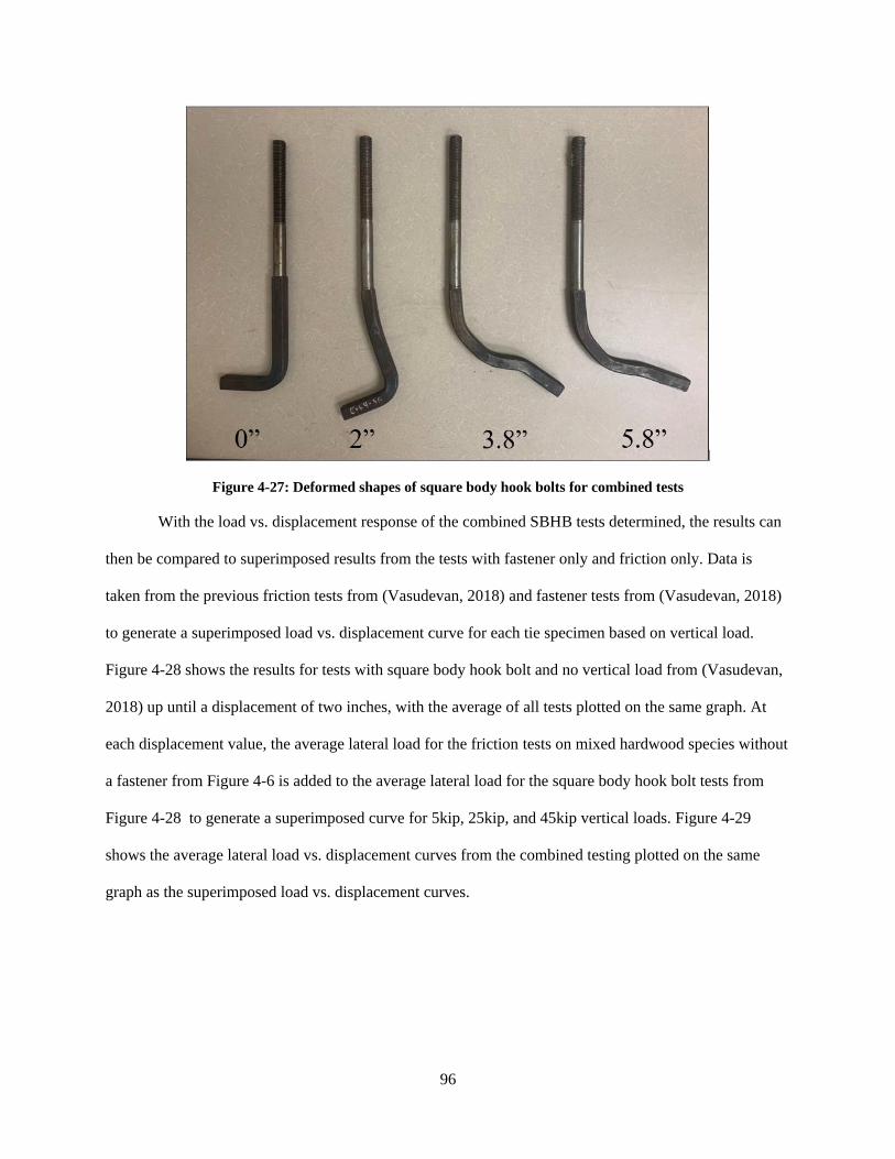
Figure 4-27: Deformed shapes of square body hook bolts for combined tests ........................................... 96
Figure 4-28: Lateral load vs. displacement for square body hook bolts (Vasudevan, 2018) ...................... 97
Figure 4-29: Experimental results vs. superimposed friction and square body hook bolt .......................... 97
Figure 4-30: Lateral load vs. displacement of all combined tests with forged hook bolt ........................... 99
Figure 4-31: Lateral load vs. displacement response to failure of forged hook bolt ................................... 99
Figure 4-32: Forged hook bolt engaging with flange (left) and at fracture (right) ................................... 100
Figure 4-33: Deformed shapes of forged hook bolts for combined tests .................................................. 100
Figure 4-34: Lateral load vs. displacement for forged hook bolts with no vertical load (Vasudevan, 2018)
.................................................................................................................................................................. 101
Figure 4-35: Experimental results vs. superimposed friction and forged hook bolt ................................. 102
Figure 4-36: Lateral load vs. displacement of tests with Quick-Set Anchor and vertical load ................. 103
Figure 4-37: Lateral load vs. displacement of Quick-Set Anchors to 2-inch displacement (Vasudevan,
2018) ......................................................................................................................................................... 104
Figure 4-38: Experimental results vs. superimposed friction and Quick-Set Anchor .............................. 105
Figure 4-39: Relative displacement of tie to girder vs. actuator displacement for entire dapped tests ..... 106
Figure 4-40: Experimental relative tie displacement vs. approximated equation ..................................... 107
Figure 4-41: Lateral load vs. displacement of dapped tests up to 2-inch displacement ............................ 108
Figure 4-42: Lateral load vs. displacement of dapped ties up to 0.5-inch displacement .......................... 108
Figure 4-43: Drawing of dapped tie specimen (Vasudevan, 2018)........................................................... 110
Figure 4-44: Lateral load vs. displacement of dapped ties containing square body hook bolt ................. 111
Figure 4-45: Bi-linear approximation for southern pine tie with 45kip vertical load ............................... 113
Figure 4-46: Experimental data vs. -2SD approximation for combined SBHB ........................................ 115
Figure 4-47: Experimental data vs. -2SD approximation for combined FHB .......................................... 116
Figure 4-48: Experimental data vs. -2SD approximation for combined QSA .......................................... 117
Page 12
xii
Figure 4-49: Experimental data vs. -2SD approximation for dapped ties ................................................. 119
Figure 4-50: Elevation view of full-size dapped railroad tie with shear planes ........................................ 120
Figure 4-51: Example rail seat reactions for ties spaced at 16 inches subjected to two axle loads .......... 121
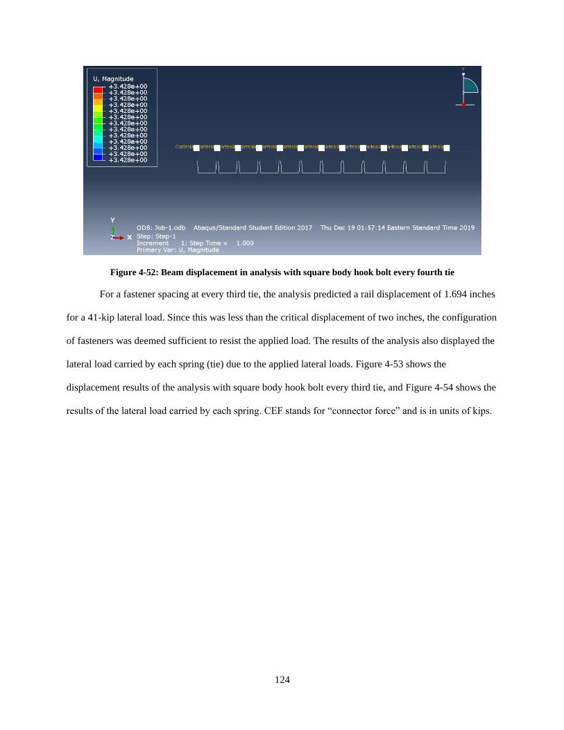
Figure 4-52: Beam displacement in analysis with square body hook bolt every fourth tie ...................... 124
Figure 4-53: Beam displacement in analysis with square body hook bolt every third tie ........................ 125
Figure 4-54: Forces in each spring from finite element analysis .............................................................. 125
Figure 4-55: Wheel to rail loads in kips (from 2010 AREMA Manual Chapter 30: Ties) [7] .................. 127
Page 13
xiii
List of Tables
Table 2-1: Data for dynamic axle loads (all values in kip)(Tobias et al., 2002) ......................................... 15
Table 2-2: Results from TTCI study of current freight car axle loads (Rakoczy & Nowak, 2018) ............ 16
Table 2-3: Nominal vertical wheel loads from AREMA Manual (AREMA, 2017b) ................................. 16
Table 4-1: Average and -2SD coefficients of static friction ....................................................................... 86
Table 4-2: Average and -2SD coefficients of kinetic friction ..................................................................... 87
Table 4-3: Dimensions of tested dapped tie samples with no vertical load or fastener (Vasudevan, 2018)
.................................................................................................................................................................. 109
Table 4-4: Rail seat reactions from Winkler equations ............................................................................. 121
Table 4-5: Example displacement and lateral load points for input into ABAQUS ................................. 123
Table 4-6: Recommended fastener spacing from analysis ........................................................................ 128
Page 14
xiv
ACKNOWLEDGEMENTS
There are many people who helped me throughout this entire research project whom I would like
to thank. Without them, this thesis would not have been possible.
First, I would like to thank Dr. Matthew Hebdon for his continued support and guidance
throughout the entire project. Thank you for believing in me to do the work for this project and
for giving advice throughout the process. I learned a lot along the way.
I would also like to thank lab assistants Garrett Blankenship and Brett Farmer for providing
significant help with getting specimens ready for testing, including helping cut specimens and
transporting them to desired locations. Additionally, I would like to thank Dr. David Mokarem
for help he provided as the structural engineering lab director.
Many thanks are owed to fellow graduate students for their help in testing, particularly Ryan
Stevens, Sam Sherry, Japsimran Singh, and Raul Avellaneda. Without your help and guidance in
running tests and getting equipment ready to run tests, I would not have been able to get all
testing done on time. Thanks is also owed to Colton Keene, Adrian Tola, Trai Nguyen, and Eric
Bianchi for providing help with finite element analysis for this project.
Thank you as well to Dr. Matthew Eatherton and Dr. Ioannis Koutromanos for serving on my
committee and providing project advice along the way.
Finally, I would like to thank my family for their support throughout the entire process.
Page 15
1
CHAPTER 1: INTRODUCTION AND BACKGROUND
1.1 Background and Scope
The primary goal of this research was to determine the lateral resistance of ties on open-deck, plate
girder railroad bridges with flat surfaces. Railroad bridges are typically constructed with either open-deck
bridges or ballasted deck bridges. In the case of open-deck bridges, the railroad crossties are supported
directly by the superstructure. Up until the early 1960’s, bridges were fabricated from riveted built-up
members, which commonly had rivet heads on the top vertical surface of the primary girders. When
crossties were placed on these riveted members, the rivets were impressed into the wood and resulted in
load resistance between the surface of the girder and the surface of the tie. While the lateral resistance of
ties was not evaluated with riveted members, it was commonly acknowledged that the rivets assisted in
preventing movement between the crosstie and girder. Since the 1960’s, most bridges are constructed from
welded built-up members and result in a flat surface supporting the crossties. It is recognized that modern
bridges with flat surfaces on the top flange of supporting members, or smooth-top girders, do not have the
same inter-planar resistance as legacy riveted structures.
Crossties are typically attached to steel plate girders with deck tie fasteners, either in the form of
hook bolts or spring clips. These fasteners also provide lateral resistance for the crossties by bearing against
the flange of the bridge girders. Fasteners are not installed at every tie, however, and can vary in installation
from every other tie to every fourth tie. Typically, during the design of open-deck bridges, the spacing of
these fasteners is arbitrarily selected based upon common owner practices and, as such, varies for different
railroads. Minimal research has been conducted to quantify the lateral capacity of the different types of
crosstie fasteners that are typically used. Additionally, although there has been extensive research
performed on the lateral capacity of ballasted railroad track, minimal research has been performed to
quantify the overall lateral resistance of ties on open-deck plate girder bridges with smooth tops.
Page 16
2
The American Railway Engineers and Maintenance of Way Association (AREMA) manual
includes only a brief section regarding the design and spacing of fasteners to connect crossties to steel plate
girders. Chapter 15 Section 8.3.2.1 of the manual states that for plate girders with rivets on the top flange,
“maximum longitudinal spacing of [fastener anchors] shall be at every 4th tie, but not to exceed 4’-8” centers
(AREMA, 2017a).” However, for plate girders with smooth top flanges containing no rivets, the same
section of the manual states that “consideration should be given to reducing the spacing of anchorages” and
that “the amount of reduction depends upon the amount of lateral and longitudinal force produced, and the
ability of the deck-to-span interface to transmit the force based on the relative smoothness of the interface
(AREMA, 2017a) .” Since the spacing requirement specification for smooth-top girders is not clear, this
has led to inconsistencies in fastener spacing amongst different open-deck bridges.
Open-deck bridges are characterized by ties that rest directly on the steel supporting elements
(girders) and connected by a fastener such as a hook bolt. These types of bridges are still used often,
especially when new bridges are being constructed on top of existing substructures since open-deck
bridges have less dead weight, which can help prevent overloading or creep of a foundation (Unsworth,
2017). Open-deck bridges also have the lowest construction costs and can drain freely, but require more
maintenance than a ballasted bridge deck (Unsworth, 2017). Figure 1-1 shows the cross-section of a
typical open-deck railroad bridge and can be contrasted with Figure 1-2 showing a typical ballasted-deck
railroad bridge. The crossties are typically supported on top of two steel plate girders and fastened to the
top flange of the plate girders with a hook bolt (further described in Section 1.3).
Page 17
3
Figure 1-1: Open-deck railway bridge (Unsworth, 2017)
Figure 1-2: Ballasted-deck railway bridge (Unsworth, 2017)
1.2 Objectives
The primary objective of this research was to experimentally determine the lateral capacity of
timber railroad ties on open-deck plate girder bridges and develop a design aid to assist engineers in
determining a suitable fastener spacing. The three main contributions to the lateral resistance of a tie on
an open-deck bridge were identified as friction resistance between the tie and top girder flange due to
Page 18
4
vertical load from train axle, resistance provided by fastener bearing against the girder flange, and
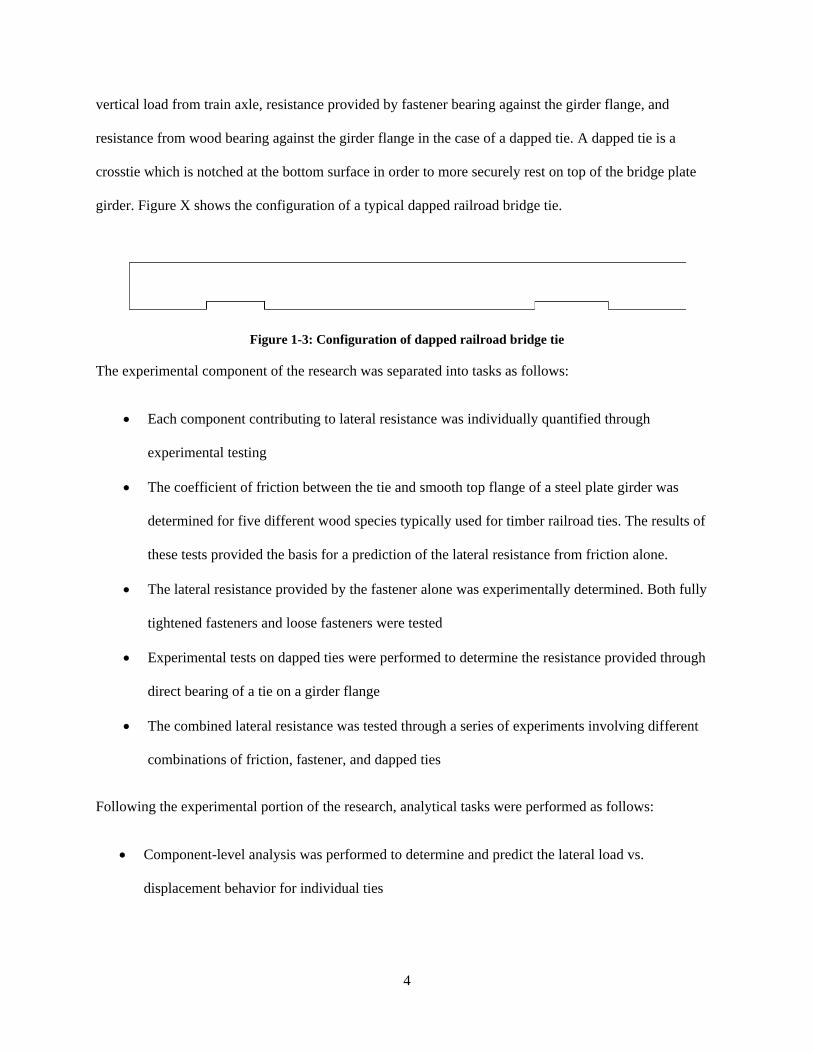
resistance from wood bearing against the girder flange in the case of a dapped tie. A dapped tie is a
crosstie which is notched at the bottom surface in order to more securely rest on top of the bridge plate
girder. Figure X shows the configuration of a typical dapped railroad bridge tie.
Figure 1-3: Configuration of dapped railroad bridge tie
The experimental component of the research was separated into tasks as follows:
• Each component contributing to lateral resistance was individually quantified through
experimental testing
• The coefficient of friction between the tie and smooth top flange of a steel plate girder was
determined for five different wood species typically used for timber railroad ties. The results of
these tests provided the basis for a prediction of the lateral resistance from friction alone.
• The lateral resistance provided by the fastener alone was experimentally determined. Both fully
tightened fasteners and loose fasteners were tested
• Experimental tests on dapped ties were performed to determine the resistance provided through
direct bearing of a tie on a girder flange
• The combined lateral resistance was tested through a series of experiments involving different
combinations of friction, fastener, and dapped ties
Following the experimental portion of the research, analytical tasks were performed as follows:
• Component-level analysis was performed to determine and predict the lateral load vs.
displacement behavior for individual ties
Page 19
5
• Finite element models were created to analyze the system behavior of a bridge with crossties, axle
loads, lateral loads, and resistance from friction and fastener
• The results of the experimental tests and global analysis models were used to create a preliminary
design aid intended to identify appropriate fastener spacing on a bridge
1.3 Overall Approach
Structural testing was performed to experimentally quantify lateral resistance of different tie
configurations. Results from the testing were used to create equations for predicting the lateral stiffness of
different ties. With these lateral stiffness equations, a finite element analysis was performed to determine
a required spacing for ties based on applied lateral and vertical loads from a train.
1.4 Scope
The project was limited to open-deck bridges with timber railroad ties and smooth top flange steel
plate girders. Testing was limited to five different species of wood: Beech, Sycamore, Southern Pine,
Oak, and Douglas-fir, and three different types of fasteners: square body hook bolts, forged hook bolts,
and Quick-Set Anchor.
Square body hook bolts and forged hook bolts are similar in the fact that they are installed in a
railroad tie through a 1-inch diameter pre-drilled hole, and hook onto the top flange of the bridge girder.
Both bolts have an “L” shape with the vertical portion extending up through the railroad tie and horizontal
hook portion bearing against the top flange of the girder. The square body hook bolt is characterized by a
shaft and hook with a square cross-section while the forged hook bolt has a round shaft and hook. The
hook for the square body hook bolt has a uniform thickness while the forged hook bolt has a tapered
thickness. Each of the two types of hook bolts can be seen in Figure 1-4. The hook bolt is attached on the
top of the tie with a washer and nut.
Page 20
6
Figure 1-4: Square body hook bolt (left) and forged hook bolt (right)
The Quick-Set Anchor utilizes a hook bolt shaped similarly to a forged hook bolt, but is unlike
the first two types of fasteners because rather than being installed through an individual railroad tie, it
passes through the gap between adjacent ties, and is bolted to a 14-inch long bracket that is attached at the
top of two ties. The hook bolt threads through a hole in the bracket and is tightened with both a washer
and two nuts. The hook bolt grips the bottom of the top flange of a bridge girder with the help of a lock
plate. When installed, the hook bolt is angled inward 15 degrees to limit lateral and vertical movement of
the deck. Figure 1-5 shows the different components of the Quick-Set assembly and how it is installed on
an open-deck bridge. The Quick-Set Anchor was introduced to the market in 2014 and claimed many
advantages during the installation process. Installing a Quick-Set Anchor on a bridge is easier and quicker
than installing traditional hook bolts because there is no need to drill a hole through the entire tie, and it
can be installed from above the deck rather than below (“Patented Quick-Set Hook Bolt System,” 2017).
Page 21
7
Figure 1-5: Left - Quick-Set anchor assembly ((Vasudevan, 2018)), Middle - Quick-Set hook bolt, Right -
Quick-Set anchor and bracket installed on ties ((“Patented Quick-Set Hook Bolt System,” 2017))
1.4.1 Crossties
Wood is a non-uniform material and its properties vary from species to species. Understanding
the mechanical and physical properties of common wood species was essential for predicting lateral
resistance characteristics of timber crossties. It was also important to understand the size and spacing of
typical timber railroad ties.
1.4.2 Species and Treatment
Wood is the most commonly used material for railroad crossties. Timber makes up approximately
93% of the market for ties installed in North America, while concrete ties are about a 6.5% share, and
steel or plastic/composite ties make up just a 0.5% share (Railway Tie Association, 2019). Wood is used
more often than other materials since it is a renewable resource, a dependable material, has a significant
service life when properly treated, and is generally more economical. Since wood can deteriorate over
time due to decay fungi, insects, and marine borers, timber crossties are treated with chemical
preservatives for protection. Research in this area found that the most common preservative for timber
ties is a creosote solution, which can also be blended with a heavy petroleum oil (Webb, Webb, & Smith,
2016). As of 2016, creosote solutions represented over 90% of preservatives used to treat wood crossties
(Webb et al., 2016).
Page 22
8
The three most important structural properties of timber crossties are their strength—both parallel
and perpendicular to the grain—and flexural strength. Wood is an anisotropic material, meaning its
mechanical properties vary in different directions. The stiffness and compressive strength of wood are not
the same in the direction parallel to the grain as in the direction perpendicular to the grain. Additionally,
wood properties vary based on species. Wood is grouped into two main categories: hardwoods and
softwoods. The two different categories have different physical and mechanical properties which affect
both strength and durability. For example, hardwood species contain vessels that make it easier to
penetrate the surface with preservatives, while softwoods have elongated cells called tracheids that
provide mechanical support. However, hardwood species are not always harder than softwood species
from a structural standpoint. (Webb et al., 2016).
While there are many different species of wood used for crossties, the most commonly used
species are oaks; mixed hardwoods such as maple, beech, sycamore, and hickories; and softwoods such as
Douglas-fir, hemlocks, true firs, and pine (Webb et al., 2016). The species of crossties tested for this
project were beech, sycamore, oak, southern pine, and Douglas-Fir, since these are some of the most
commonly used species. Using both hardwood and softwood species also allowed for an analysis of how
the classification of wood can affect its lateral resistance on an open-deck bridge.
1.4.3 Size and Spacing
The typical size and spacing of railroad bride crossties differ from standard crossties. According
to section 3.1.1.3.1 of Chapter 30 of the AREMA manual, the standard dimensions for a non-bridge
crosstie are 8-inches-wide by 8.5-inches-high by 8.5-to-9 feet long (AREMA, 2017b). The standard
spacing is 19.5 inches center to center (AREMA, 2017b). The AREMA specification for bridge ties, on
the other hand, specified a minimum of 10 feet long and at least 8 inches wide. Typically, bridge ties are
between 8-to-12 inches wide and have a clear spacing of up to 6 inches. This means the center-to-center
spacing of bridge ties is typically between 12 and 18 inches. The height of a bridge tie is dependent on
girder spacing, spacing bars, and walkway requirements, but is typically around 12 inches (AREMA,
Page 23
9
2017b). Figure 1-6 shows how the standard tie sizes from AREMA compare for a typical crosstie and a
bridge crosstie. The bridge tie is both wider, taller, and longer to resist flexural loads.
Figure 1-6: AREMA standard sizes for typical and bridge railroad ties
Page 24
10
CHAPTER 2: LITERATURE REVIEW
A review of past literature for determination of vertical and lateral loads, lateral resistance of
railroad ties, and analysis methods for the design of railroad bridges was performed. This chapter will
describe the different types of loads that a train axle imposes on a railroad track, the fundamentals of train
wheel dynamics, methods for determining lateral resistance of railroad crossties, and analysis techniques
for determining how much vertical and lateral load each railroad tie must resist.
2.1 Train Wheel Dynamics
Before quantifying train loads and determining lateral resistance of railroad track, it was
necessary to have fundamental knowledge of the wheel-to-rail dynamics for a train. Review of literature
describing train wheel-to-rail dynamics was thus necessary for this research.
The dynamics of train wheels is concisely described in a book titled The Railway Track and its
Long-Term Behavior by K. Tzanakakis. According to Tzanakakis, train locomotives and cars have axles,
which have two wheels rigidly connected on either end (Tzanakakis, 2013). Typically, two axles are
connected to a truck (bogie), which is the component of the train car that guides the train on the rails and
provides stable operation. A train car body typically has two trucks. The profiles of the train wheels are
conical rather than flat, allowing for proper steering of the wheelset (axle and wheels)(Tzanakakis, 2013).
When a train is navigating a curve, the wheel on the outside rail (high rail) will have to cover more
distance than the wheel on the inside rail (low rail). The conical shape of the wheel causes the diameter of
the outer wheel to be greater than the diameter of the inner wheel, allowing the wheelset to be forced back
to the center of the track during a curve so that the train can be steered properly (Tzanakakis, 2013). Since
the wheelset is rigid, meaning the wheels rotate at the same angular velocity, when one wheel has a larger
diameter it will cover a greater linear distance than the wheel with smaller diameter, thus allowing the
outer wheel on a curve to move faster than the inner wheel(Tzanakakis, 2013). Figure 2-1 shows the
wheelset of a train and the conical shape of the wheels. The left image shows a wheelset on a straight
Page 25
11
portion of track, where the diameters of the wheels are equal. The right image shows a wheelset on a
curved portion of track, where the rolling diameter of the left wheel (outer wheel) is greater than the
rolling diameter of the right wheel. The flange of the left wheel may also bear against the rail during the
curve.
Figure 2-1: Wheelset on straight track (left) vs. wheelset on curved track (right) (Tzanakakis, 2013)
As the train moves along a curve, both longitudinal and lateral creep forces are generated between
the wheel and rail, as well as a normal force between the wheel flange and the rail. Lateral creep forces
develop on both the low and high rail due to lateral slip of the wheel while the direction of the wheelset
changes along a curve (Nilmani, 2011). A normal flange force is developed if a train is moving fast
enough or travelling on a sharp curve, where lateral creep may not be enough force to allow proper
steering of the vehicle. The flange force is created when the wheel bears against the flange of the high
rail, causing significant lateral force on the rail (Nilmani, 2011). When lateral load is generated due to
creep or flange force, this load is transmitted from the rail to the crossties below.
2.1.1 Wheel Hunting
Although the largest lateral forces on railroad track are generated on curves, railway vehicles can
also have lateral movement on straight tracks, according to AREMA. This movement is referred to as
hunting and occurs when a train reaches a certain critical speed. Hunting is characterized by a continuous
sinusoidal oscillation of the wheelset, and occurs due to “dynamic instability of the vehicle caused by
interaction between the conicity of the wheels, forces acting between wheels and rails, and action of the
Page 26
12
truck suspension”(Wickens, 2010).” Essentially, when a wheelset is hunting, the self-centering action
caused by conicity of the wheels becomes unstable and results in oscillation. The oscillation ultimately
applies lateral load to the rail, meaning that lateral load should be quantified and considered for straight
track as well as curved.
2.2 Rail Loads
Determining the anticipated loads on a railroad bridge is essential for design of the structural
components. A railroad bridge can experience loading in different directions, including lateral, vertical,
and longitudinal. This paper focused mainly on the vertical and lateral loads on the bridge ties since these
are the loads that will affect the design in the lateral direction. This warranted a review of literature
detailing the type and magnitude of the different loads which can be imposed on a rail, primarily the
AREMA manual.
The majority of loads imposed on a railway structure is dynamic loads. According to N.F. Doyle
in his work titled Railway Track Design: A Review of Current Practice Occasional Paper, the dynamic
vertical and lateral loads on a rail structure are commonly expressed as a function of the static loads
through the use of an empirically determined “dynamic impact factor (N.F. Doyle, 1980).” The
relationship between dynamic and static loads is given by the equation
𝑃 = ∅𝑃𝑠 (1)
where P is the design wheel load, Ps is the static wheel load, and Ø is the dimensionless dynamic impact
factor (N.F. Doyle, 1980). Currently there are a variety of methods for determining the dynamic impact
factor, each of which depends on the speed of the train. For most methods, the factor ranges from one to
three, and increases either linearly or parabolically as a function of train speed (Van Dyk, Edwards,
Dersch, Ruppert, & Barkan, 2017).
Page 27
13
2.2.1 Vertical Dead Loads
The vertical loads on individual railroad ties on an open-deck bridge consist of both dead and live
loads. In the case of railroad bridges, the live load on the ties is significantly higher than the dead load,
since the weight of the moving train is much greater than the dead load from the rail and fasteners on each
individual tie. For ties on an open-deck railroad bridge, the dead load consists of just the track rails, inside
guardrails, and their rail fastenings. According to Chapter 15 of the AREMA Manual for Steel Structures,
the dead load should be taken as 200 lb. per linear foot for each track (AREMA, 2017a). If railroad ties
are spaced at 14 inches apart in a bridge, this equates to a dead load of just 0.233 kips per tie per rail. This
load is significantly smaller than the load from train wheels, as will be seen in Sections 2.2.2 and 2.2.3
2.2.2 Cooper E80 and Alternative Live Load
The vertical live load on bridge ties depends on the weight of each train wheel and the dynamic
impact effects for the train. Heavier trains which are moving at a faster speed will have a much greater
vertical live load than trains moving at a slower speed due to dynamic effects. AREMA Chapter 15
establishes two baselines for determining the design live load for bridges: The Cooper E80 Load and the
Alternate Live Load. Both baselines establish design axle loads and spacings for a typical train with
locomotives and cars. Figure 2-2 shows the Cooper E80 and Figure 2-3 shows the Alternative Live load
configuration from the AREMA Manual. The 80 in the “E80” refers to the 80-kip weight of locomotive
drive axles, while the Alternate method uses 100-kip axles (Sorgenfrei & Marianos Jr., 2000). The
Cooper E80 system has been adopted because it provides a universal system for calculating live loads
from trains, for which all other load configurations can be compared (Sorgenfrei & Marianos Jr., 2000).
Both Cooper E80 and Alternate live load establish a common axle spacing of 5 feet for both
locomotives and cars. Loads from different train configurations can be compared to the Cooper E80 and
Alternate live load configurations by calculating Equivalent Cooper E Loadings (ECELs) and Equivalent
Alternate Loadings (EALs). Since both the Cooper E80 and Alternate loading are design loads, they
should be greater than the actual loads from trains in service.
Page 28
14
Figure 2-2: Cooper E80 live load configuration from AREMA Chapter 15 (AREMA, 2017a)
Figure 2-3: Alternate Live Load configuration from AREMA Chapter 15 (AREMA, 2017a)
2.2.3 Actual Vertical Train Live Loads
Recent studies have been conducted to determine actual car and axle load for heavy freight trains
currently running, in order to test the validity of the Cooper E80 and Alternate Loading since freight
trains continue to become heavier and more powerful. An influential study of heavy freight loads was
conducted by Tobias et. al. in 2002. where dynamic loads were recorded for over 35,000 rail cars from
three of the general freight types for trains (Tobias, Foutch, & Choros, 2002). The mean and maximum
axle loads from the study for each of the different types of freight are shown in Table 2-1.
Page 29
15
Table 2-1: Data for dynamic axle loads (all values in kip)(Tobias et al., 2002)
Freight Type
Avg. Axle
Load
Max Axle
Load
Avg. Wheel
Load
Max Wheel
Load
Coal hopper 66 109 33.2 54.5
Coal hopper (91tons) 64 109 31.8 54.5
Coal hopper (100tons) 70 106 35.2 52.9
Ballast hopper 69 107 34.6 53.3
Potash hopper 68 95 34.2 47.5
Four-axle intermodal 36 68 18.0 33.9
Autorack 46 71 22.8 35.5
Five-pack intermodal 34 91 17.1 45.5
Two-axle intermodal 36 68 18.2 33.9
Four-axle mixed
freight 20 95 10.1 47.5
Six-axle locomotive 69 96 34.4 48.0
Four-axle locomotive 70 103 35.2 51.5
The data from Tobias et. al show that the maximum load per wheel for common freight cars and
locomotives fell between 34 kips and 55 kips. Using this data, equivalent Cooper E and Alternative
loadings (ECELs and EALs) for simple bridge spans were also calculated using the maximum measured
loads from the coal hoppers (which produced the highest axle loads). From these calculations it was
concluded that the loading environment from the actual rail cars was approaching the Cooper E80 design
loads, which are supposed to always exceed the actual vertical dynamic loads (Tobias et al., 2002). The
results from Tobias et. al indicate that with increase in weight of freight cars, the design live loads will
probably need to be increased in the future (Tobias et al., 2002).
A more recent study of the current vertical loads from heavy freight cars was conducted by TTCI
in 2017, where the dynamic load was recorded for four different types of fully loaded, 130-ton gross
weight cars (Rakoczy & Nowak, 2018). The mean and maximum axle loads from the TTCI study are
shown in Table 2-2. The results show that the axle loads for these cars all exceeded 80 kips (40 kips per
wheel). Similar to Van Dyk et al., commentary on the study by Rakoczy & Nowak explained how the
actual vertical loads of trains continue to grow over the years and are now exceeding the design Cooper
E80 loads (Rakoczy & Nowak, 2018).
Page 30
16
Table 2-2: Results from TTCI study of current freight car axle loads (Rakoczy & Nowak, 2018)
Chapter 30 of the 2017 AREMA Design Manual used data from studies such as Van Dyk et al., and
Rakoczy & Nowak to generate a consolidated graph of average vertical wheel loads from different types
of trains. Table 2-3 is shows that consolidated graph and displays the average nominal vertical wheel
loads from different types of train cars.
Table 2-3: Nominal vertical wheel loads from AREMA Manual (AREMA, 2017b)
The data from the two studies, along with the tabulated values from the AREMA Manual validate the
choice of using 45kips as the maximum vertical wheel load applied to the tie specimens for this research.
Since the maximum wheel loads for heavy freight tended to be around 40-50 kips, using 45kips for tests
Page 31
17
served as a realistic maximum vertical load that may be applied to a railroad bridge tie. Additionally, the
justification for using 5 kips as the lower bound vertical load is displayed in Table 2-3, which shows how
the data predicts a mean value of 7 kips for an unloaded freight car, likely the lowest vertical wheel load
that will be produced from a standard train. Analyzing studies like these are also important because they
indicate that railway design may change in future years due to the increasing weight of freight trains, and
this should be accounted for when attempting to determine reasonable loads that will be applied to a
railroad bridge.
2.2.4 Centrifugal Force
The AREMA Manual also describes how to deal with centrifugal force, which is the primary
lateral force occurring on a curved railway track. The centrifugal force occurs when a train is moving
along a curved track, and there is a significant lateral force that develops on the rail due to the change in
direction of the velocity of the train. The moving train transmits this centrifugal force to the rail at the
point of wheel contact, which then transmits force to the cross-ties beneath the rail (AREMA, 2003). The
centrifugal force from the train is very important to understand when determining the lateral loads that
will act on railroad crossties and fasteners on a curved railroad bridge.
The centrifugal force is a function of the vehicle load, the degree of the curve, and speed of the
vehicle while it is traversing the curve (AREMA, 2003). The degree of the curve is known based on its
geometry, and train axle load can vary based on the size of the train. The AREMA provisions for the
calculation of the centrifugal force are given in Chapter 15 of the AREMA Manual for Railway
Engineering. The provisions state that the centrifugal force for curves “shall be applied horizontally
through a point 8 feet above the top of rail measured along a line perpendicular to the plane at top of rails
and equidistant from them (AREMA, 2017a).” The centrifugal force is then calculated as a percentage of
each axle load without impact, and is given as
𝐶 = 0.00117𝑆2𝐷 (2)
Page 32
18
where C is the percentage of each axle load (centrifugal factor), S is the speed of the vehicle in miles per
hour, and D is the degree of the curve (AREMA, 2017a). This equation allows for a calculation of the
centrifugal force that is applied to the rail at each wheel during a curve if the wheel axle load is known.
The combination of the centrifugal force and vertical force from the train weight produces a
resultant force that is directed towards the outside rail of the curve. If a train is navigating a curve where
both the outside rail and inside rail are at the same elevation, the resultant force will not align with the
centerline of the track(Hook, 2017). This can be seen in Figure 2-4, which shows how the resultant force
from the lateral and vertical forces lies at a point near the outer rail, causing more weight on the outside
rail (Hook, 2017). From the figure it can also be seen that if the centrifugal force increases with respect to
the weight (this can occur with increase in speed of the train), then the resultant force will fall even
further away from the center of the track. This can be a problem if the resultant force falls outside the
outer rail, which could result in overturning of the train.
Figure 2-4: Resultant force due to weight of train and centrifugal force (Hook, 2017)
In order to reduce the likelihood of a train overturning, superelevation is often utilized, which
involves raising the outer rail slightly higher than the inside rail, and thus rotating the track slightly on its
axis. This allows for the resultant force from the weight and centrifugal force to fall more closely to the
center of the track. When a track has superelevation so that the resultant force falls on the centerline of the
Page 33
19
track, it is said to be in equilibrium position (AREMA, 2003). Typically, a curved railroad track does not
have enough superelevation to be in equilibrium, so the difference between the equilibrium elevation of
the track and actual elevation is called the underbalance (AREMA, 2003). This underbalance can be
measured and is used as a factor for determining the maximum allowable velocity of the train on a curve.
The superelevation of the railway track does not affect the magnitude of the centrifugal force, but it does
affect the point of application of the force. Regardless of superelevation, the centrifugal force will always
act perpendicular to the rail and parallel to the crossties.
2.2.5 Research on Centrifugal Wheel-to-Rail Force
Though an equation is provided for the centrifugal force from a train wheel depending on the
degree of the curve, previous research has investigated the actual lateral wheel to rail loads from a train
truck. A report by Herbert Weinstock in 1980 for the US Department of Transportation attempted to
quantify the wheel/rail force and flange force applied by train trucks navigating curved railroad track
(Herbert Weinstock, 1980). The report develops a procedure for “estimating the conservative bounds for
the wheel/rail forces resulting from curve negotiation of a rigid two-axle truck (Herbert Weinstock,
1980).” With the procedure, the report establishes a wheel to rail lateral load variation with respect to the
degree of curve. The study assumes a two-axle car with a weight of 100 kips (50 kip axle load) for
determining the lateral loads applied to the rail. Figure 2-5 shows a figure from the report describing the
lateral wheel to rail force as a function of degree curve. As can be seen from the figure, the lateral load
from a wheel can exceed 20 kips for curves with a degree greater than 20 degrees when the axle load is 50
kips. This figure shows an example for an upper bound lateral load on a rail, and can be used for
determining the lateral loads in the analysis of railroad track for determining spacing of tie fasteners.
Page 34
20
Figure 2-5: Wheel to rail forces assuming a 100-kip axle (Herbert Weinstock, 1980)
2.2.6 Moving Freight Equipment
While centrifugal effects make up the dominant lateral forces for a curved railroad bridge, there
are also lateral forces that can develop from track irregularities at the wheel-rail interface which were
described in Section 2.2.1. Although the magnitude of the lateral load due to moving equipment is
advanced in nature, its value for design purposes has been simplified with suitable equations. The
AREMA Manual quantifies these lateral forces as 25% of the heaviest axle of Cooper’s EM360 (E80)
load, and studies conducted by Otter et. al have confirmed that this specification is suitable (AREMA,
2017a). For analysis purposes, the lateral load at each axle for a straight track will be determined in this
manner.
Page 35
21
2.2.7 Impact Loading
Impact load due to the dynamic movement of a train is an important load case that is considered
for the design of the bridge’s structural components. Impact load can be due to both vertical and rocking
effects and is an important consideration for open-deck bridges. According to the AREMA Manual,
impact loading from vertical effects should be expressed as a percentage of live load applied to each rail,
and is given by the following equations:
𝐹𝑜𝑟 𝐿 100 𝑓𝑒𝑒𝑡 𝑜𝑟 𝑚𝑜𝑟𝑒: 10 +
1800
𝐿 − 40 (3)
𝐹𝑜𝑟 𝐿 𝑙𝑒𝑠𝑠 𝑡ℎ𝑎𝑛 100 𝑓𝑒𝑒𝑡: 60 −𝐿2
500
where L is the length in feet from center to center of supports for stringers or longitudinal girders
(AREMA, 2017a).
AREMA describes the impact load due to rocking effect as a “load created by transfer of load
from the wheels on one side of a car or locomotive to the other side from periodic lateral rocking of the
equipment” (AREMA, 2017a).” This load is calculated from loads applied as a vertical force couple,
with each being 20 percent of the wheel load without impact and acting downward on one rail and upward
on the other (AREMA, 2017a).
2.3 Maximum Vehicle Speed on Curves
Since the centrifugal force depends on the speed of the vehicle, it is important to determine the
speed of the train as it is moving along the curve. The equation for calculating the maximum design
speed of a train travelling a curve is specified in Chapter 6 of AREMA’s Practical Guide to Railway
Engineering. The equation is given as
𝑉𝑚𝑎𝑥 = √𝐸𝑎 + 3
0.0007𝐷 (4)
Page 36
22
where Vmax is the maximum allowable operating speed, Ea is the average elevation of the outer rail with
respect to the inside rail in inches, D is the degree of the curve in degrees, and the 3 is the amount of
underbalance, which is assumed (AREMA, 2003). This equation shows that the maximum speed can
increase with an increase in superelevation, but the higher the degree of the curve, the smaller the
maximum velocity. This maximum velocity can be used for determining the anticipated centrifugal force
of the train while it is traversing the curve.
2.4 Lateral Load (Net Axle Ratio)
A commonly used ratio for determining the maximum lateral load on a railroad track in the railroad
industry is the L/V ratio. According to literature, the L/V ratio is the lateral to vertical load ratio where
“the net lateral load applied to the track by one axle of a truck resulting from the flanging forces and the
two lateral components of the wheel/rail frictional force at both wheels on the axle are divided by the total
vertical axle load (Kish, Gopal Samavedam, & David Wormley, n.d.).” The industry establishes a limit on
the L/V ratio to prevent derailment or overturning of a train vehicle. According to the FRA, the limit on
the L/V ratio is given with the following equation:
𝐿
𝑉= 0.4 +
5
𝑉
(5)
where L/V is the net axle ratio and V is the vertical load of the axle in kips (Vehicle/Track Interaction
Safety Standards; High-Speed and High Cant Deficiency Operations, 2010). If the vertical axle load is
50 kips, then from Equation 5, the maximum allowable L/V ratio is 0.5. This means that the maximum
lateral load from a 50-kip axle would be 25 kips. This is consistent with the data found by Weinstock,
which predicted a maximum lateral wheel to rail load of just over 25 kips. This equation will be used to
determine the worst-case scenario lateral load on a curved railroad bridge depending on the vertical axle
load, V. This lateral load is assumed to be the worst-case scenario, for a bridge with a very degree of
curvature, and if a track has sufficient lateral resistance to resist these loads, then it will be considered
safe.
Page 37
23
2.5 Vertical Tie Reaction
The lateral resistance of railroad ties on a bridge are heavily influenced by friction between tie
and girder that is caused by vertical load from a train wheel. Thus, it is highly important to understand
how much vertical load is transferred to each tie from the rail when a train moves across a bridge. In this
section, a review of literature regarding the determination of the vertical force carried by a single tie is
provided. In the paper “Understanding Stresses in Rails” by Jude Igwemezie, when a point load from a
wheel is applied to the rail, the load is not only carried by a single tie but instead by multiple adjacent
ties(Igwemezie, 2007). This vertical load distribution is influenced by many parameters, which include
tie spacing, stiffness of the track support (ballast or girder), rail size, and axle spacing (Igwemezie, 2007).
There are a number of different ways to analytically model a train rail to determine the approximate
vertical load carried by each tie, some of which will be analyzed in Section 2.4.
2.5.1 Winkler Base Model
The most popular method in practice for modelling a train rail is a beam on an elastic foundation,
which was first made popular by Emil Winkler in 1867 (Tzanakakis, 2013). The Winkler Base model
operates under the assumption that the distributed reaction force of the railroad track support is linearly
proportional to the vertical rail deflection. The method uses Euler-Bernoulli beam theory and models the
rail as a beam with known bending stiffness, EI, and that is supported by a continuous elastic foundation
(Tzanakakis, 2013). The elastic foundation contains an infinite number of linear springs with known
stiffness. Figure 2-6 shows how a beam on an elastic foundation appears. Using Euler-Bernoulli beam
theory, an equation for deflection of the rail due to a point load P can be calculated with differential
equations and is given as:
𝑦(𝑥) =
−𝑃𝛽
2𝑢𝑒−𝛽𝑥 ∗ [𝑐𝑜𝑠(𝛽𝑥) + 𝑠𝑖𝑛(𝛽𝑥)]
(6)
Where:
Page 38
24
𝛽 = (𝑢
4𝐸𝐼𝑧)
1/4
(7)
For this equation, y(x) is the vertical displacement of the rail as a function of distance, x, from the point
load P, E is the modulus of elasticity of the rail, Iz is the second moment of area of the rail, and u is the
stiffness of the structure supporting the rail (Tzanakakis, 2013). Equation (6) can then be used to solve
for the vertical pressure distribution beneath the rail by multiplying the vertical displacement by the
known vertical stiffness of the supporting structure, as shown in equation (8) below:
𝐹(𝑥) = −𝑢 ∗ 𝑦(𝑥) =𝑃β
2𝑒−𝛽𝑥 ∗ [𝑐𝑜𝑠(𝛽𝑥) + 𝑠𝑖𝑛(𝛽𝑥)] (8)
where F(x) is the vertical pressure reaction at any location x from the load (Selig & Li, 1994). Equation
(8) can then be used to solve for the reaction force at each tie (often called the rail seat load) by
multiplying the pressure reaction F at the center of the tie by the spacing between each tie. This can be
represented by the equation:
𝑄𝑛 = 𝐹𝑛𝑆 (9)
where Qn is the rail seat reaction force, S is the center to center spacing of adjacent railroad ties, and Fn is
the value of the pressure found from Equation (8) at the center of the tie (Selig & Li, 1994). With these
equations, the vertical load experienced by each tie can be determined for any location and magnitude of
load, and any tie spacing.
Figure 2-6: Beam on an elastic foundation with vertical point load (Tzanakakis, 2013)
The use of Equations (8) and (9) can also produce the maximum rail seat load predicted by the Winkler
model, which is often used for the design of railroad ties. The largest force will occur directly beneath the
point load, where x = 0, which means the maximum rail seat load will become:
Page 39
25
𝐹𝑚𝑎𝑥 =𝑃𝛽𝑆
2 (10)
The Winkler equations for rail seat load can also be used for multiple point loads when there is more than
just one axle applying load to the rail. The rail seat load can is determined simply by superimposing the
displacement generated by different loads (Kerr, 2003). Figure 2-7 shows the displacement profile of a
rail predicted by the Winkler equations for two axle loads of 45 kips spaced 5 feet apart, and common
parameters of E=29000 ksi, I = 77.4 in4, and u = 9 ksi. This figure shows how the displacement profiles
due to each load can be superimposed to generate an overall displacement profile, which will be equal in
shape to the rail seat pressure profile. For the Winkler model, the parameter “u” is often referred to as the
track modulus(Selig & Li, 1994). This value is a measure of the vertical stiffness of the rail foundation
and is independent of the rail itself (Selig & Li, 1994). The track modulus value for a typical railroad
track can often be difficult to determine, because it depends on the stiffness of ballast and earth beneath
the ties, along with vertical stiffness of the tie itself (AREMA, 2017b). For an open-deck railroad bridge,
steel bridge girders make up the supporting structure, so determining the stiffness modulus of the steel
girder is essential for determining the deflection and forces in bridge ties. Railroad track on an open-deck
bridge tends to have a greater stiffness than track supported by ballast and subgrade.
A higher track modulus results in a smaller deflection but generally higher rail seat force, whereas
lower modulus has higher deflection, but the load is distributed over more ties resulting in a decrease in
load resisted by a single tie (Van Dyk, Scheppe, Edwards, Dersch, & Barkan, 2016). Therefore, rail seat
loads on open-deck bridges will be greater than that for typical ballasted railroad track.
Page 40
26
Figure 2-7: Rail deflection due to axle loads with Winkler model
2.5.2 Accuracy of Winkler Model
While the Winkler model is easy to use and has the ability to predict deflection of the rail at any
point, it has limitations that affect its overall accuracy. Since the model assumes a continuous elastic
foundation, it neglects the fact that the rail supports are actually spaced apart a discrete amount (tie
spacing) (Tzanakakis, 2013). However, despite this simplified assumption, research done by the Talbot
Committee in 1919 and Wasiutynski in 1937 has shown that the displacement calculated from Winkler is
very similar to displacement calculated from methods assuming the spring supports are spaced at discrete
distances (Kerr, 2003).
Further limitations of the Winkler model include the fact that it assumes a constant track modulus
value, while in reality the modulus may vary from tie to tie, and also assumes that the springs are
independent of each other, which is unrealistic (Sharma, 2016). The model is also limited to only static
loading, whereas in reality dynamic effects from the train can influence deflection. Despite these
limitations, a study conducted by Zakeri and Sadeghi in 2007 more recently challenged the accuracy of
the Winkler model for predicting deflection of the rail due to a vertical point load. The study conducted
-0.09
-0.07
-0.05
-0.03
-0.01
0.01
0.03
0 50 100 150 200 250 300 350 400
Rai
l Def
lect
ion
(in
)
Distance along rail (in)
Axle Load 1 Axle Load 2 Superimposed
P=45kip P=45kip
Page 41
27
field tests by applying a 48.5-kip point load to a rail and measuring the vertical displacement of the rail at
known distances from the load (Zakeri & Sadeghi, 2007). Since the track modulus of the rail was known,
the experimental displacements were then compared to displacements predicted by the Winkler equation.
The authors concluded that the use of the Winkler model is justified for determining deflections, since the
differences in deflection between the experimental and theoretical data did not exceed more than 30%
(Zakeri & Sadeghi, 2007).
Though the Winkler model has proven to be valid for determining rail deflection, its use for
determining rail seat force has been proven inaccurate by experimental tests. A study by Kerr and
Shenton in 1986 showed that predictions from the Winkler model underestimated the maximum rail seat
force by 30% (Kerr & Shenton III, 1986). The authors attributed this inaccuracy to the Winkler
assumption that contact pressures are proportional to rail deflections, as described by Equation (8). The
report found that, in reality, as wheel loads increase, the stiffness of the base increases, meaning the load
vs. deflection response of a ballast base is bi-linear instead of simply linear. Due to this finding, Kerr
recommended that the rail seat force values calculated from the Winkler equation be multiplied by 1.5 for
design purposes (Kerr, 2003). This realization has influenced subsequent predictions for the maximum
rail seat load. While it has been shown that the Winkler model is accurate for predicting rail deflection, it
must be altered in order to accurately calculate the force that is distributed to each tie from the rail.
2.5.3 AREMA, Talbot, and Kerr Equations
Since the adoption of the Winkler method, several equations and codes have subsequently been
generated for quickly calculating the maximum rail seat force due to vertical wheel load. Some of these
methods overcome the limitations of the Winkler model by including dynamic impact loads in the
analysis, along with accounting for the nonlinearity of the track stiffness. These methods involve a
generalized equation for determining the maximum rail seat load based on axle load and tie spacing.
Three of the most common methods developed are the AREMA equation, Talbot equations, and Kerr
equations (Van Dyk et al., 2016). The AREMA equation depends only on tie spacing and wheel axle
Page 42
28
load, while the Talbot equation also depends on track modulus, train speed, and stiffness properties of the
rail, and the Kerr equation further depends on the diameter of the train wheel. The Talbot and Kerr
equations are derived from the beam on elastic foundation theory, and also include a dynamic factor used
to increase the static train loading. The AREMA, Talbot, and Kerr equations, respectively, are given as:
𝑅 =(1.5626𝑆 + 12.811)𝑃
100 (11)
𝑅 =
[𝑃 + 0.01𝑃(𝑉 − 5)] ∗ 𝑆 ∗ (𝑢
4𝐸𝐼)
1/4
2
(12)
𝑅 =
(1 + 0.33𝑉𝐷
) ∗ 𝑃 ∗ 𝑆 ∗ (𝑢
4𝐸𝐼)
1/4
2
(13)
where R is the maximum rail seat load in pounds, S is tie spacing in inches, P is the static wheel load in
pounds, V is train speed in mph, u is track modulus in psi, E is modulus of elasticity of the rail in psi, I is
moment of inertia of the rail in in4, and D is the wheel diameter (Van Dyk et al., 2016). A 2016 study by
Van Dyk et. al. used experimental testing to make a comparison and determine the accuracy of the three
methods. Results from the study found that all methods predicted a lower rail seat load for stiff support
conditions, but in general predicted a slightly higher rail seat load than recorded in the field (Van Dyk et
al., 2016). This study further emphasizes the fact that the stiffness of the support conditions is highly
influential when determining rail seat load.
While maximum rail seat force is important for designing railroad ties, this study is primarily
concerned with the rail seat force in each tie due to a wheel load. Since lateral resistance will increase
with higher rail seat reactions, a smaller rail seat reaction was conservative for this analysis. Therefore,
Page 43
29
based on the findings of the previous studies mentioned in this chapter, the Winkler model will serve as a
suitable method for this study for predicting vertical loads on each tie.
2.6 Track Lateral Resistance
The lateral resistance of standard railroad track embedded in ballast has been extensively
quantified and researched, however, it has not been as well researched for open-deck bridges where the
railroad crossties are not embedded in ballast. When considering methods for quantifying lateral
resistance of open-deck bridges, it is important to study and apply the methods used for determining the
lateral resistance of ballasted railroad track.
2.6.1 Contributions to Lateral Resistance
Railroad track has three in-plane resistance characteristics: lateral, longitudinal, and torsional, and
one vertical out-of-plane resistance characteristic. Each of these characteristics can be idealized as a
“spring” load-deflection response (Kish, 2011). Lateral resistance for standard railroad track is provided
by the ballast and has three main contributions: bottom friction between tie and ballast, side friction, and
end/shoulder restraint. Bottom friction is influenced by the type of tie and weight, side friction by the type
of crib content, and shoulder restraint by the end ballast geometry (Kish, 2011). Figure 2-8 shows the
three main contributors to lateral resistance and how much of the overall resistance they typically account
for (Kish, 2011).
Figure 2-8: Components of lateral resistance for ballasted railroad track (Kish, 2011)
The bottom friction between railroad tie and ballast is typically the leading contributor to lateral
resistance and depends on both vertical load and friction coefficient parameter, µ. In the case of heavy
Page 44
30
axle loads, however, dynamic uplift can occur which can greatly reduce the bottom friction resistance
(Kish, 2011). As shown in Figure 2-9, ties that fall directly under the load have increased resistance, but
ties that are not loaded can have decreased resistance, making the end and side friction even more
important. The concept of dynamic uplift is consistent with vertical rail deflections predicted by Winkler,
as evidenced in Figure 2-9 where there is a predicted upward displacement in certain ties that are not near
the vertical load.
Figure 2-9: Concept of dynamic uplift in railroad track (Kish, 2011)
The components of lateral resistance presented by Kish can be applied to open-deck railroad
bridges by considering similar contributions for ties fastened to bridge girders. The friction between tie
and girder represents the bottom friction component of lateral resistance. Lateral resistance provided by a
fastener, and/or bearing resistance provided by a dapped tie represents the end resistance. Since there is
no ballast on a railroad bridge, there is no side friction to contribute to lateral resistance. Therefore, the
overall lateral resistance for an open-deck bridge can be considered a sum of the resistance from fastener,
dap, and tie-girder friction due to vertical load. The concept of dynamic uplift may also occur for ties on
a railroad bridge, so it should be considered when determining bottom friction resistance.
2.6.2 Experimental Methods for Determining Lateral Resistance
In previous research, there have been two main experimental methods for determining lateral
track resistance. The first is the Track Lateral Pull Test (TLPT), where the total resistance is obtained by
laterally loading an entire track and measuring the deformation curve of a section of track. The second is
a Single Tie Push Test (STPT) where a single tie is separated from the rail and displaced laterally. For the
Page 45
31
TLPT, the lateral resistance is the applied force divided by the distance that the track is deformed, while
for the STPT, the resistance is the applied force divided by the displacement of the individual tie itself
(Zarembski, 2016). Track lateral resistance can thus be represented as either force per length of track or
force per tie.
The single tie push test is the easiest test to perform and is the most common means for obtaining
track lateral resistance. Other advantages of the STPT are that the resistance values determined are not
affected by rail rigidity or rail longitudinal force since the tie is separated from the rail (Samavedam,
Kanaan, Pietrak, Kish, & Sluz, 1995). The main disadvantage of the STPT, however, is that it only
provides resistance for a single tie, and tie resistance can vary along the length, whereas the TLPT
provides a direct measurement of track lateral resistance over a long length (Samavedam et al., 1995).
Thus, the TLPT is more accurate for determining the overall track lateral resistance.
A study conducted by Choros, Zarembski, and Gitlin in 1980 attempted to quantify lateral track
shift and determine the differences in results produced by TLPTs and STPTs. For this experiment, a full-
scale test track was constructed. Four 100-kip capacity hydraulic jacks were used to apply vertical load
and two 50-kip capacity hydraulic jacks were used to apply lateral loads to a loading bolster that
represented a 100-ton capacity freight car. Initially, TLPTs were performed with vertical load applied to
the bolster and then lateral load was applied and increased until reaching a predetermined lateral
deflection of the tie directly at the loading point, after which the lateral load was recorded. This process
was repeated until the tie at the loading point displaced a total of one inch. Deflection values were also
recorded at other ties to obtain an overall track displacement curve and track lateral resistance.
Additionally, STPTs were performed on individual ties that had been removed from the track, where
lateral load was applied to the tie in the same process as for the TLPT until two inches of total
displacement. The lateral stiffness for both the TLPTs and STPTs was determined by fitting a line to the
linear portion of the load vs. displacement plots generated from the tests (Choros, Zarembski, & Gitlin,
1980).
Page 46
32
Results from the TLPTs indicated that the track deflected in the shape of a damped sine wave,
and the lateral stiffness of the track increased with an increase in vertical load (Choros et al., 1980). The
study also found that the single tie push test results produced a greater lateral stiffness than the TLPTs.
The paper ultimately concluded that while the TLPT was more representative of “real track” conditions,
single tie push tests can (and should) be used for determining lateral resistance, as long as a correlation
factor is determined (Choros et al., 1980).
2.6.3 Predicting Lateral Resistance from STPT
Since the Single Tie Push Test has been proven to not be a completely accurate representation of
track lateral stiffness, a correlation factor or method needs to be implemented to use data from an STPT to
predict track resistance. Choros, Zarembski, and Gitlin identified that a correlation factor needs to be
determined in order to make this conversion but did not give information for what this factor might be. A
later study conducted in 1995 by the Federal Railroad Administration (Samavedam et al., 1995) attempted
to determine the correct correlation factor. This study performed both STPTs and TLPTs on railroad ties
in the same track. From the data, the report concluded that the TLPT response can be directly determined
by taking average resistance values from STPTs. The process for converting STPT data to TLPT data
involves treating the rails as a beam on a nonlinear elastic foundation and taking into account the
nonlinear lateral spring stiffnesses determined by the STPTs (Samavedam et al., 1995). Essentially, each
tie can be represented by a nonlinear spring that supports the beam rail in the lateral direction, and an
analysis can be done to measure the lateral displacement of the rail due to a point load. The study was
influential because it proved that it was unnecessary to use an empirical correlation factor, and determined
that STPTs can be performed to accurately predict the overall lateral response of a railway track.
For this report, a variation of the single tie push test was performed due to being easier, cheaper,
and more affordable than a full track laboratory test. The STPTs were performed to determine the
nonlinear lateral stiffness of an individual bridge tie. Then, using the same methods as presented in
Samavedam et al., the data from the STPTs were converted to an overall track response. Similar to
Page 47
33
Choros, Zarembski, and Gitlin, lateral load was applied to the tie up until two inches of displacement, and
the lateral load was recorded at different deflections to generate a load vs. displacement curve.
Page 48
34
CHAPTER 3: METHODOLOGY
3.1 Structural Test Setup
The structural test setup used for the experiments in this project simulated one half of a typical
railroad bridge, utilizing only one-third of a full-length railroad tie and one simulated bridge girder. A
detailed drawing of the test setup is shown in Figure 3-1. For further details regarding the structural test
setup, refer to Appendix C.
Figure 3-1: Rendering of test setup
The test frame had two W21x62 columns, which were spaced at 8 feet, and had a height of 15
feet. Two W21x62 crosshead beams were connected to the columns by six 0.75-inch-diameter A325
bolts at each connection, 13 feet above the ground. A 220-kip capacity vertically oriented MTS actuator
was attached to the crosshead beams through a 21-inch-long W21x101 stub section. An 18-inch x13-inch
x 2-inch steel plate was bolted to the end of the vertical actuator to serve as the surface over which the
vertical load was applied.
Page 49
35
A five-foot-long W27x235 steel beam was situated on the ground directly beneath the vertical
actuator and between the two columns to serve as the simulated girder for the test setup. The vertical
actuator was thus able to apply vertical load directly above the flange of the girder and simulate vertical
load from the rail of a railroad bridge. Another 5-foot-long W27x235 beam was bolted to the floor
perpendicular to the first girder in order to support a 110-kip capacity horizontal MTS actuator. Both of
the girder sections had two 0.5-inch-thick vertical stiffeners on each side of the web spaced at two feet
apart. The horizontal actuator that rested on top of the W27x235 girder was used to apply a lateral load to
the face of a wooden railroad tie specimen that lied on top of and perpendicular to the simulated bridge
girder. Figure 3-2 shows the entire test setup with both the vertical and horizontal actuators.
Figure 3-2: Photo of structural test setup
Since the simulated bridge girder was not bolted to the ground, it was braced in two different
ways to prevent weak axis bending and translation during testing. Two L3x3x1/2 bracing members were
connected to each end of the girder as shown in Figure 3-1 and bolted to the ground. Additionally, a beam
oriented perpendicular to the simulated bridge girder was bolted to the girder web on one end with four
Page 50
36
bolts, and bolted to a reaction block on the other end in order to further brace the girder from rotating
during testing. The reaction block was bolted to a strong floor, and also served as a structure for which the
horizontal actuator could be chained to in order to prevent uplift. The bracing beam and reaction block are
shown in Figure 3-3.
Figure 3-3: Bracing beam and reaction block for structural test setup
In order to make sure the horizontal actuator applied load in the same plane as the face of the tie
specimen, a 36-inch x14-inch x 1-inch steel plate was supported by steel blocks directly on top of the
flange of the simulated girder section. This allowed the plate to be raised 5-inches above the actual flange
of the W27X235 girder, so each tie specimen could rest on top of the plate and be at the same height as
the horizontal actuator. The plate was bolted to the girder flange with four bolts at each corner. Figure 3-4
shows how the plate raises above the flange of the actual simulated bridge girder.
Page 51
37
Figure 3-4: Steel plate bolted to the W27X235 simulated bridge girder
3.2 Friction Testing
The friction resistance between the railroad tie and flange of the bridge girder is one of the main
contributors to the overall lateral resistance of a railroad tie on an open-deck bridge. Friction resistance
can be simply calculated as the product of the normal force applied to the specimen as a result of vertical
load from a train wheel, and the coefficient of friction between the tie and girder flange. The simplified
equation for friction force is given as
𝐹𝑓𝑟𝑖𝑐𝑡𝑖𝑜𝑛 = 𝜇𝑁 (14)
where Ffriction is the friction force, µ is the coefficient of friction, and N is the normal force. In the case of
railroad bridge ties, if the coefficient of friction can be quantified for a type of wood, then the lateral
resistance of a bridge tie with no fastener or dap can be predicted with equation (14).
3.2.1 Friction Test Methods
In order to determine the coefficient of friction for railroad ties on smooth-top bridge girders, tie
specimens with no dap or fastener were tested with the test setup described in Section 3.1. A specimen
with a length of roughly 3.5 feet was placed on the test girder and loaded vertically with the 220-kip
Page 52
38
capacity actuator. The specimen was positioned so that its overhang was approximately 20 inches off the
edge of the flange in the direction facing the horizontal actuator. This was done because bridge survey
observations showed that the edge of a bridge tie on an open-deck bridge is typically 27 to 28 inches
away from the point of application of normal force (train rail). Since the flange of the W27X235 girder
was 14 inches wide, a 20-inch overhang would result in a 27-inch distance from the center of the actuator
plate to the edge of the tie.
Since testing sought to determine friction between just the tie and girder only, the tests required
there to be no friction between the vertical actuator plate and tie. As a result, a combination of rollers and
steel plates were used to eliminate friction between the top of the tie specimen and actuator. The setup of
rollers and steel plates is shown in Figure 3-5. A 12-inch x18-inch x 0.75-inch steel plate was placed on
top of the tie specimen directly beneath the actuator plate, and four 13-inch-long by 1-inch diameter steel
rollers were spaced equally along the plate. A second steel plate of the same size was placed on top of the
rollers, and the vertical actuator applies load to this upper plate. The rollers were greased to reduce
friction even further. Additionally, as a safety measure in case any of the rollers disengage from under
the load, angles were clamped to the specimen on either side of the actuator plate, as shown in Figure 3-5.
Page 53
39
Figure 3-5: Friction test setup with steel plates, rollers, and angles
To allow the specimen to move laterally in the same plane, two 12-inch-long L3x3x1/2 angles
were clamped to the girder plate on either side of specimen, which can be seen in Figure 3-5. A specified
vertical load was then applied to the specimen and treated as a static load. The vertical load was measured
with a load cell connected to the actuator. With vertical load applied, the horizontal actuator was moved
so that it contacted the end of the tie specimen, as seen in Figure 3-5. For all friction tests, the horizontal
actuator simulating lateral load displaced at 1 inch per minute for a total of two minutes and displacement
was measured with an LVDT. This results in a 2 inch overall lateral displacement of the actuator since 2
inches was determined to be a displacement significant enough to cause a train derailment in a bridge.
Load applied by the horizontal actuator was measured with a load cell, and since the test was
displacement controlled, the lateral load vs. displacement response of the horizontal actuator was
returned. The data from the lateral load vs. displacement provided insight on the lateral resistance
provided by friction.
Page 54
40
3.2.2 Wood Species Tested
For this research, railroad crossties from five different wood species were tested in order to
investigate whether species of wood has an effect on the lateral resistance provided by friction between
the tie and steel bridge girder while a train is moving across a bridge. For this project, railroad crossties
made from a mixed hardwood species of beech and sycamore, southern pine, oak, and Douglas-fir were
tested to determine how the friction coefficient between tie and girder varies with type of railroad tie.
3.2.3 Beech and Sycamore
The first batch of ties donated for testing were identified as beech and sycamore ties. Friction
testing on the beech and sycamore ties was performed by Vasudevan. As classified by the Railway Tie
Association, both beech and sycamore fall under a larger group known as “mixed hardwoods”, which is
the second most used group of wood for railroad ties behind oak. Mixed hardwoods are higher in density
and material surface hardness than southern pine but slightly lower than oak. They also tend to have a
lower rail seat compressive strength than other species(Webb et al., 2016). Both beech and sycamore are
labelled by the Railroad Tie Association as species that are most difficult to treat with creosote
preservative(Webb et al., 2016).
The beech and sycamore ties were donated by Norfolk Southern Railroad Company and are
shown in Figure 3-6. The bridge ties were removed from a bridge in North Carolina after being in service
for 15 years. The length of individual ties varied from 11 feet to 12 feet. The cross-sectional dimensions
also varied between 7.5 inches to 8 inches for the horizontal dimension and 10 inches to 12 inches for the
vertical dimension. The ties had two daps (notches at the bottom of the tie so that it can rest securely on
the bridge girder) on either end. The dap length varied from 13 inches to 23 inches and the dap height
varied from 0.25 inches to 2.5 inches. The mixed species ties had a low creosote preservative retention,
although some specimens had a coating of grease on the outside.
Page 55
41
Figure 3-6: Beech and sycamore bridge ties (Vasudevan, 2018)
The mixed hardwood bridge ties were cut into 3.5-foot-long segments with a chainsaw to be
prepared for testing. All ties had tie plates and bearing pads held in place by railroad spikes as shown in
Figure 3-7. All components of the rail fastening system such as bearing pads, tie plates, hook bolts, and
railroad spikes were removed from the ties prior to testing. Railroad spikes were pried from the wood
using a railroad spike puller.
Figure 3-7: Tie plates, bearing pads, and railroad spikes on top of tie (Vasudevan, 2018)
3.2.4 Southern Pine
The second type of wood species tested was southern yellow pine. Southern pine is classified as a
softwood species by the Railway Tie Association, and is less dense than other wood species such as oak
or mixed hardwoods (Webb et al., 2016). Southern pine also has a lower surface hardness than oak and
mixed hardwoods, but a higher modulus of elasticity and modulus of rupture. The southern pine ties used
for testing were donated by CSX. These ties were previously used in an existing railroad viaduct and were
Page 56
42
donated after being removed from service. In total, 15 southern pine crossties were donated, all
approximately 120 inches in length. Each crosstie had a 0.75-inch thick dap on both sides, as is shown in
Figure 3-8.
Since the friction testing needed to be done on un-dapped specimens, the southern pine crossties
were cut into thirds using a chainsaw. Five cross-ties were cut in total, so that the ~40” middle section cut
from the tie could be used as a specimen for testing in the loading apparatus. The tops of each of the
specimens had been weathered as shown in Figure 3-8, with uneven surfaces created by wood chipping
away. The rest of the surfaces of the specimens were relatively smooth and contained minimal
preservatives such as creosote.
Figure 3-8: Southern Pine railroad ties donated by CSX
The five southern pine specimens tested ranged from 3’-3” to 3’-5” in length, 9.5 inches to 10.5
inches in height, and 9.75 inches to 10.3 inches in width. To differentiate between each, all specimens
were labelled “SPX” with SP standing for southern pine and X corresponding to a different number from
1 to 5. All specimens except for SP4 were taken from the middle of the full-length crosstie, meaning four
out of five did not have a dap. In the case of SP4, there was a 1’-5” long, 0.75-inch-deep dap in the
middle of the specimen. In order to both save time in cutting another tie and to see how the lateral
Page 57
43
resistance might differ on a different side of the tie, specimen SP4 was turned upside-down on the girder
so that the dap was at the top. This left the weathered, un-dapped side of the specimen as the side
contacting the girder. The top was then shimmed with 0.75-inch steel plates in order for the 12-inch x18-
inch steel plate connected to the vertical actuator to rest flat on the top of the tie.
Five tests were performed on each of the five southern pine specimens at five different vertical
loads. All tested specimens are shown in Figure 3-9. The vertical loads for testing were 5 kip, 15kip,
25kip, 35kip, and 45kip.
Figure 3-9: Five southern pine specimens cut for testing
3.2.5 Oak Species
The third species of wood that was tested was oak. According to the Railway Tie Administration,
oak is a hardwood and the most common wood species used for railroad crossties. Oak as a construction
material has a very high hardness (higher than southern pine and mixed hardwoods), as well as a high
density. The high hardness and ability to be chemically treated allow oak railroad ties to be highly durable
and have a long service life (Webb et al., 2016).
Both new and old oak railroad ties were donated to Virginia Tech for testing. Two full-size
brand-new oak railroad ties were donated to Virginia Tech by CSX, both of which were about 10 feet in
Page 58
44
length. Both were covered extensively by a dark creosote and had a dap on either end. Similar to the
southern pine ties, the new oak ties were cut into ~42-inch pieces with a chainsaw in order to be tested.
Four testable specimens were able to be cut from the ties. The specimens were marked with a white pencil
and labelled “OX” with the “O” corresponding to oak and X corresponding to a different number, 1
through 4. Figure 3-10 shows the four new oak specimens that were prepared for testing, along with a
closer look at how much preservative was retained on the surface of the ties. The new oak specimens
ranged from 10-inches to 11-3/16 inches in height, while maintaining a consistent 10-inch width.
Figure 3-10: Four new oak specimens tested (right) and close up of creosote preservative on ties (left)
Additionally, about 10 old oak railroad ties were donated by CSX, each of which had a
significantly lower creosote retention than the brand-new oak ties. The ties were a dark brown color rather
than dark black and were all about 7 inches in width and 9 inches in height. All ties had a dap on either
end, so for testing, specimens were cut from the centers of the ties. In total, five specimens were cut from
five different old oak ties, and labelled “OOX” with X ranging from 1 to 5. The five old oak railroad tie
specimens cut for testing are shown in Figure 3-11.
Page 59
45
Figure 3-11: Five old oak specimens tested (left) and close up of old oak surface (right)
3.2.6 Douglas-fir Species
The final type of wood tested for this project was Douglas-fir. Similar to southern pine, Douglas-
fir is classified as a softwood. According to the Railway Tie Administration, Douglas-fir is a relatively
popular species of wood used for railroad ties primarily in Canada and the western United States. It has
also been used extensively for bridge timber (Webb et al., 2016). Douglas-fir has a lower density than
oak, mixed hardwoods, and southern pine, and a material surface hardness lower than hardwoods and oak
but slightly greater than southern pine (Webb et al., 2016).
Approximately 10 Douglas-fir railroad ties were donated to Virginia Tech by Union Pacific. The
ties were old railroad ties that had been in service on a bridge in Council Bluffs, Iowa, and are shown in
Figure 3-12.
Page 60
46
Figure 3-12: Douglas-fir ties donated for testing
The ties were 12 feet in length on average, and had cross-sectional dimensions of 10 inches in
width and 12 inches in height, similar to the mixed hardwood ties. Each tie had a dap on either end. Four
ties were cut with a chainsaw to acquire a ~42-inch un-dapped tie specimen from the center of the tie.
The ties were each labelled “DFX” with DF corresponding to Douglas-fir and X ranging from 1 to 4
depending on the order of testing. All ties had a very low creosote retention.
3.3 Material Testing
Compression testing both perpendicular and parallel to the grain of wood was performed for all
different species of railroad ties tested for this project. This was done in order to identify important
material properties for the wood such as compressive strength and modulus of elasticity in both grain
directions. Additionally, each type of wood used was examined under a microscope in order to verify the
species of wood.
3.3.1 Compression Testing
All wood was tested according to ASTM D143: Standard Test Methods for Small Clear
Specimens of Timber. One crosstie of each different species used for testing was cut into 4-inch long
segments using a bandsaw. The segments were then further shaped with a table saw into wood specimens
Page 61
47
that were 4 inches x 1-inch x 1-inch. Each specimen was oriented so that the grains ran parallel to the 4-
inch long dimension. For each species, 20 specimens were cut to be tested and each were labelled and
measured to obtain exact dimensions.
A universal testing machine (UTM) was used to test each of the specimens. 10 specimens of each
species were loaded parallel to the grain and 10 specimens loaded perpendicular to the grain as seen in
Figure 3-13. The specimens parallel to the grain were each compressed at a rate of 0.012 inches per
minute until reaching a maximum displacement of 1 inch or when the load dropped by more than 100 lbs.
from the ultimate load. The specimens perpendicular to the grain were also loaded at a 0.012 inches per
minute rate until a maximum displacement of 1 inch. The load vs. displacement curve for each test was
plotted, and then converted to stress vs. strain diagram based on the original cross-sectional dimensions
and length of each specimen. The stress-strain curves allowed for a compressive strength and modulus of
elasticity to be calculated for each species of wood in each direction.
Figure 3-13: Compression test parallel to grain (left) and perpendicular to grain (right)
Page 62
48
3.4 Combined Friction and Fastener Tests
The previous phase of this project involved separating the lateral resistance from friction between
tie and girder, and lateral resistance from fasteners installed in the tie. This was done by running two
separate types of tests: tests with a fastener attached to the specimen but no vertical load applied, and tests
with vertical load applied but with no fastener installed. The overall resistance of an un-dapped railroad
tie with a fastener is a combination of the two components, but it is not explicitly clear that the overall
resistance is simply the sum of the two. Therefore, in order to analyze how both the fastener and friction
work together to provide resistance, tests were run with specimens having both fasteners installed, and
vertical load applied. These tests were referred to as “combined tests” since they combined the two
components of friction and fastener. The same three types of fasteners tested in the first phase of the
project were all tested for the second phase: square body hook bolts, forged hook bolts, and Quick-Set
Anchors.
3.4.1 Combined Square Body Hook Bolt and Forged Hook Bolt Tests
The test method for the combined friction and fastener tests was the same as for the friction tests
described in Chapter 3.3, except that a fastener was installed to the tie. For installing the square body
hook bolts and forged hook bolts, a 1-inch diameter hole was drilled through the center of the specimen
using a Heavy-Duty Hole Hawg Drill at a distance of 20 inches from the edge of the specimen in the long
direction. The specimen was then placed on the test girder plate and a hook bolt was placed through the
hole until the hook engaged with the bottom of the top flange of the girder as seen in Figure 3-14. The
hook bolt was then secured to the girder with a bridge washer and tightened with a 0.75-inch hexagonal
nut that was snug tightened using a wrench.
Page 63
49
Figure 3-14: Square body hook bolt (left) and forged hook bolt (right) engaged with the test girder plate
As seen in Figure 3-15, when the hook bolt was installed, it protruded out from the top of the tie
by a few inches. Since the fastener protruded at a point that was underneath the vertical actuator plate, an
additional wooden block needed to be added on top of the tie so that the fastener did not affect the bottom
steel plate that supported the rollers for the friction tests. The wooden block and overall setup can be seen
in Figure 3-16. With the setup the same as shown in Figure 3-16, the vertical load can be applied and the
test is the same as for the friction tests, with the specimen being displaced at 1 inch per minute.
For both the square body hook bolts and forged hook bolts, combined tests were performed at
vertical loads of 5 kips, 25 kips, and 45kips. The tie specimens used were un-dapped specimens, meaning
that the specimens laid flat on the girder, and no lateral resistance was provided from bearing of wood
against the girder flange. The species of wood used for the specimens was the same beech/sycamore used
for the first phase. Figure 3-17 shows what the combined tests with vertical load and fastener looked like
during testing.
Page 64
50
Figure 3-15: Bridge washer and nut used to tighten hook bolt
Figure 3-16: Wooden block used to allow steel plate to lay above hook bolt
Page 65
51
Figure 3-17: Combined friction and fastener test setup
A total of eight tests were run with square body hook bolts. Two tests were run until 2 inches of
displacement at each of the three vertical loads, while two tests were run until failure of the hook bolt at
45kip vertical load. The specimens for testing ranged from 3’-1” to 3’-6” in length, 1’-0” in height, and
about 10 inches in width. Each specimen was labelled “CFFX” with “CFF” standing for “combined
friction and fastener” and X ranging from 1 to 8. During each test, the load vs. displacement
characteristics were measured and plotted to gain a better understanding of the behavior.
As for the forged hook bolts, a total of seven combined friction and fastener tests were performed.
Two tests were run with a 5-kip vertical load to two inches of displacement, two tests with 25-kip vertical
load to two inches of displacement, and three tests with 45-kip vertical load to failure of the hook bolt.
The specimens for testing ranged from 3’-3” to 3’-8” in length, 9.5” to 10.25” in width, and 11.25” to
12.25” in height. Each specimen was labelled CFFX with X ranging from 9 to 15. Same as for the tests
with the square body hook bolts, the lateral load vs. displacement response was recorded to analyze the
overall lateral capacity.
Page 66
52
3.4.2 Combined Friction and Quick-Set Anchor Tests
The fastener tests with Quick-Set Anchors were different from the tests with square body and
forged hook bolts because two tie specimens were loaded at the same time as opposed to just one. The
Quick-Set Anchor assembly needed to be assembled on the ground before lifting onto the test girder. Two
tie specimens were spaced at five inches apart on the ground since the typical clear spacing for bridge ties
is between four and six inches. The ends of both specimens were flushed with each other so that the
horizontal actuator could apply load equally to both ties. The steel Quick-Set bracket (as seen in Figure
3-18) was then placed on top of the ties at about 22 inches from the end of the loaded edge of the
specimens. Holes with 0.375-inch diameter were then drilled in the ties in the location of the holes on the
Quick-Set bracket. Two 0.625-inch x 7.5-inch high strength lag screws were then pushed through each of
the two pre-drilled holes using an air wrench in order to fasten the bracket to the ties. Figure 3-18 shows
the Quick-Set bracket secured to two adjacent specimens with the lag screws.
With the bracket secured, the tie specimens were lifted into the test setup with a crane so that they
hung about 20 inches over the edge of the girder plate. A Quick-Set hook bolt with a lock plate was then
inserted through the hole in the middle of the bracket between the two ties. The hook bolt is shown in
Figure 3-18. Once the hook bolt was in position so that the hook engages with the bottom of the plate, a
0.75-inch diameter washer and two 0.75-inch diameter hexagonal nuts were snug tightened with a wrench
at the top of the bracket in order to secure the hook bolt to the girder. The overall setup can be seen in
Figure 3-19.
Page 67
53
Figure 3-18: Quick-Set bracket installed on specimens (left) and Quick-Set hook bolt with lock plate (right)
Figure 3-19: Quick-Set Anchor setup
For the Quick-Set Anchor tests with vertical load applied, a mechanism to distribute the vertical
load to both specimens was required. To distribute the load and separate the bracket from the vertical
actuator during loading, wood blocks were stacked on top of the two specimens as seen in Figure 3-20.
The wood was stacked high enough so that a 24-inch x 24-inch x 1-inch steel plate could be placed on top
of the wood to support the rollers. Since the plate was two feet wide, the load from the actuator, which
was transferred to the plate, was distributed to both specimens evenly. With the rollers spaced equally
Page 68
54
apart on the steel plate, the load was applied in the same way as the previous friction tests with a 12-inch
x18-inch x1-inch steel plate on top of the rollers. The tests were then run with the same 1 inch per minute
displacement rate as the friction tests until either a maximum displacement of 4.5 inches was reached, or
failure of the hook bolt occurred.
Figure 3-20: Combined friction and Quick-Set Anchor setup with wood blocks and larger steel plate on top
For the combined friction and Quick-Set Anchor tests, a total of eight tests were performed.
Three tests were run with 5-kip and 25-kip vertical load, and two tests were run with 45-kip vertical load.
The tie specimens used for the tests were Beech/Sycamore species ties, and were the same specimens
used for testing of the combined forged hook bolts tests. A total of eight different ties and four Quick-Set
brackets (four setups) were used for the eight tests.
3.5 Dapped Tie Testing
In the previous phase of the project, dapped tie samples were used for testing the contribution to
lateral resistance from a dap only, with no vertical load applied nor hook bolt installed to the tie. For this
phase of the research, tests were performed on dapped specimens with both vertical load and fastener in
Page 69
55
order to see whether friction and fastener resistance affect the overall resistance of a dapped tie specimen.
Dapped specimen testing was performed on the mixed hardwood ties, only.
For the tests, the dapped portion of the tie was placed on the steel plate such that the end facing
the horizontal actuator was approximately 18-20 inches from the edge of the steel plate as shown in
Figure 3-21. In order to induce a shear failure of wood in the dapped tie, each tie specimen was notched at
a distance of 12 inches away from the girder flange as shown in Figure 3-21. Introducing this notch
prevented moment in the tie during loading while also keeping the length of the shear plane constant. For
testing with no vertical load or fastener, five dapped ties were notched and tested. The specimens were
loaded by the horizontal actuator displacing at a constant rate of 1 inch per minute until a dap failure
occurred. The tie width and dap depth were recorded before testing.
Figure 3-21: Dapped tie with 1-inch thick notch (Vasudevan, 2018)
3.6 Relative Displacement Reading
For the majority of the tests performed in this project, the displacement of the tie was assumed to
be the same as the displacement of the horizontal actuator, which was measured by an LVDT connected
to the actuator. After analyzing videos of the tests, an observation was made that despite bracing from the
beam and two angles, the simulated bridge girder rotated about its strong axis when load was being
Page 70
56
applied. This meant that the displacement reading for the tests was not actually the relative displacement
between the tie and girder since it did not account for this slight rotation.
In order to correct the load vs. displacement results for the previous tests, additional tests were
conducted with an alternative method to measure the relative displacement between the tie and girder
flange. For these tests, an angled steel plate was screwed to one side of the tie specimen. Two lasers were
attached with C-clamps to a vertical HSS tube, with one laser pointing at the steel plate serving as the
simulated top flange, and one laser pointing at the angled steel plate, attached to the side of the tie, as
shown in Figure 3-22.
The lasers were connected to a CR1000 data logger so that the displacement of both the tie and
the girder flange could be measured at every 0.1 second during the test. The relative displacement could
then be determined simply by subtracting the displacement of the flange from the displacement of the tie
at each recording. This data allowed for a plot of lateral tie displacement vs. time, which could then be
used to correct the load vs. displacement data for the previous tests using the actuator displacement. Since
the original tests returned actuator force and displacement at every 0.1 seconds, the displacement readings
from the actuator could simply be replaced by the relative displacement readings from the lasers to
generate a plot of actuator force vs. relative tie displacement.
Page 71
57
Figure 3-22: Lasers used to measure relative displacement of tie and flange
Tests with the lasers were run on one Douglas fir specimen at all five of the vertical loads tested
for friction testing (5kip, 15kip, 25kip, 35kip and 45kip) and the relative displacement vs. time graphs
were plotted for each. It was assumed that the relative displacement vs. time curve for the Douglas fir ties
would be very similar for the other species at the same vertical loads. Therefore, the results from the tests
on Douglas fir were used to correct all load vs. displacement curves for the friction tests on all species.
Additionally, tests with the laser displacement readings were run on Douglas fir specimens with a
hook bolt installed. Three tests were run with a square body hook bolt: one with no vertical load, one with
25-kip vertical load, and one with 45-kip vertical load. Two tests were run with a Quick-Set Anchor
installed, one with no vertical load and one with 25kip vertical load. The relative displacement readings
from the square body hook bolt tests were assumed to be very similar to readings for forged hook bolt
tests, so the previous load vs. displacement plots for the tests with square body hook bolt, forged hook
bolt, and Quick-Set Anchors were updated accordingly.
Page 72
58
Finally, a test with the lasers was run on a dapped specimen. The test was conducted with a 45kip
vertical load and square body hook bolt. It was assumed that the relative displacement readings for the
dapped tests with vertical load and square body hook bolt up until dap failure would be similar to relative
displacement readings of dapped tests with no vertical load or fastener.
3.7 Cleaning Lateral Load vs. Displacement Data
For some of the tests, during application of lateral load the simulated bridge girder would slip
beneath the tie, causing a large oscillation in lateral load vs. lateral displacement. The consistent
“slipping” that occurred caused the measured load vs. displacement response to be messy and not
representative of the actual behavior of the load during the test. In order to clean this data, a Loess
regression algorithm with a smoothing parameter of 0.1 was used to generate a smooth-fit curve through
the data points. The Loess method is a common method used to fit a smooth line to a series of noisy data
values. Figure 3-23 shows an example of how the Loess regression was used to generate a smooth lateral
load vs. displacement curve.
In order to more succinctly display the lateral load vs. displacement data of multiple tests run with
similar conditions (such as two different friction tests run at a 5-kip vertical load), average lateral load vs.
displacement curves were determined. For each test, the lateral load measured by the horizontal actuator
was returned for every 0.1 seconds during the test. As described in Chapter 3.6, the lateral displacement
vs. time is assumed to be the same for similar tests. For example, the lateral displacement vs. time was
assumed to be equal for all friction tests run with a 5-kip vertical load. Therefore, the average load vs.
displacement curve could be generated by averaging all lateral load values occurring at the same time,
since they were all at the same displacement for similar tests. This allowed for an average curve to be
generated that still maintained the same shape as the individual tests and gave an accurate but concise
representation of the test results.
Page 73
59
Figure 3-23: Example of Loess regression to smooth data
While the average lateral load vs. displacement curves were useful for predicting the actual
behavior of the tests, for design purposes it was also useful to generate a curve that represented the lateral
load two standard deviations less than the average lateral load. Assuming that the lateral resistance of an
individual tie within a population of similar railroad ties (i.e. same species, same fastener type) was
normally distributed, a curve that is 2 standard deviations less than the mean curve will represent a lateral
resistance that is less than 95% of ties. Thus, this would generate a conservative lateral load vs.
displacement curve that could be used for design purposes on a railroad.
Since similar tests recorded the lateral load at the same displacements, the standard deviation of
the lateral load for all tests in the sample of tests can be computed with the following equation:
𝜎 = √∑ (𝐹𝑖 − 𝐹𝑎𝑣𝑔)2𝑁
𝑖=1
𝑁 − 1 (15)
where σ is the sample standard deviation of lateral load at a specific displacement , N is the number of
tests in the sample, Fi is the lateral load of the test at the specific displacement, and Favg is the average
0
5
10
15
20
25
30
35
0 0.2 0.4 0.6 0.8 1 1.2 1.4 1.6 1.8 2
Lat
eral
Load
(kip
)
Lateral Displacement of tie (in)
Experimental Curve Smooth Curve with Loess
Page 74
60
lateral load of all tests in the sample at that specific displacement. With the standard deviation of lateral
load determined, a -2SD force for each displacement value can be generated by multiplying the standard
deviation by two and subtracting from the average lateral load at each displacement. In order to make sure
the curve maintains the same shape, a ratio is generated by dividing the -2SD force at each displacement
by the average force at that displacement. For example, if the average lateral load at a displacement of
0.25 inches is 5.00 kips, and the standard deviation of lateral load at 0.25-inch displacement is 1.00 kips,
the -2SD force becomes 5.00kip – 2*(1.00kip) = 3 kips. The ratio of -2SD load to average load is thus
3kip / 5kip = 0.60 at a displacement of 0.25 inches. This ratio value is then averaged amongst all data
points (displacement values). With an average ratio determined, the -2SD lateral load vs. displacement
curve is generated by multiplying each average load value by the average ratio.
3.8 Methods of Analysis
This section details the methods for determining the lateral stiffness of an individual railroad tie, and
how this data is used to predict the overall strength of a section of railroad track.
3.8.1 Lateral Stiffness Approximations
The goal of experimental testing was to ultimately provide a recommendation for fastener spacing
which would allow railroads to be more consistent with their spacing and only provide fasteners when
necessary to provide lateral resistance. In order to do this, equations had to be generated for predicting the
lateral stiffness of a section of railroad track. Testing for this research provided lateral load vs. lateral
displacement curves for many different types of railroad ties, including un-dapped ties with no fastener,
un-dapped ties with a fastener, dapped ties with no fastener and dapped ties with a fastener. To accurately
predict the lateral stiffness of an individual railroad tie, approximate equations could be generated based
on the minus-2 standard deviation lateral load vs. displacement curves from the experimental tests. The
minus-2 standard deviation curves were used since they were conservative approximations which is
important from a structural design standpoint.
Page 75
61
For the majority of the experimental tests, the lateral load vs. displacement response could be
approximated with either a bi-linear curve or a tri-linear curve. As will be shown in Chapter 4, friction
tests on un-dapped ties with no fastener produced a bi-linear lateral load vs. displacement curve, while
tests on un-dapped ties with both a fastener and vertical load produced a tri-linear curve. After solving
for the approximate minus-2 standard deviation curve from the experimental tests, the curve itself was
split into its different linear portions. For example, for the friction tests, the curve was split into an initial
linear increase in load portion and a constant zero stiffness portion. With the curves split accordingly, a
best-fit line was approximated for each linear portion of the load vs. displacement curve. The equations of
each approximated line were returned in the form of
𝐹(𝑥) = 𝑚𝑥 + 𝐶𝑜𝑛𝑠𝑡𝑎𝑛𝑡 (16)
where F(x) is the lateral load in kips, x is the lateral displacement in inches, m is the slope of the line in
kips/inch, and the “Constant” is the y-intercept of the line in kips. The lateral displacement where the
lines intersect could be determined by setting the equations equal to each other and solving for
displacement. This analysis resulted in a piecewise approximation for predicting the lateral resistance of
a railroad tie based on its lateral displacement.
When attempting to predict the lateral stiffness of a railroad tie on an open-deck bridge, it is
important to understand the lateral loads which will be applied to the tie and what type of lateral
resistance the tie will have. Figure 3-24 shows a typical cross-section of an open-deck railroad bridge
with un-dapped ties and the types of forces that are applied while a train is moving across. Figure 3-25
further shows what an open-deck bridge might look like in 3 dimensions, showing how different ties have
different lateral resistance depending on if a hook bolt is installed or not.
Page 76
62
Figure 3-24: Typical cross-section of open-deck railroad bridge with forces
The wheels of the train apply concentrated loads to the rail in both the vertical and lateral
direction. The vertical wheel load is transferred from the rail to the tie to the primary supporting girders.
This will create a normal force between the tie and girder flange which creates friction resistance. As a
train is moving across the bridge, especially on a curved bridge, the wheels apply lateral load to the top of
the rail, which is then transferred to the tie which is attached to the rail. From Figure 3-24, if a bridge is
curving to the right, then the centrifugal force will cause lateral loads to be acting to the left.
As per Figure 3-24, for an un-dapped railroad tie with a fastener on both ends, the lateral loads
will be resisted by a combination of friction due to normal force between tie and girder, and fastener
bearing against the flange. When lateral forces are acting in the direction as shown in Figure 3-24, only
the inner fastener will be bearing against the flange as the tie tries to displace in the direction of the lateral
forces. The outer fastener will provide lateral resistance if the bolt is tight and there is tension between the
hook bolt and the bottom of the top flange.
Page 77
63
Figure 3-25: Typical open-deck plate girder bridge with fasteners in every third tie
Since not all fasteners are always tightly bolted to the tie, the lateral resistance of the outer
fastener was ignored in this analysis for conservatism. Therefore, the overall resistance of the tie seen in
Figure 3-24 was considered a combination of friction resistance from the outer girder, and friction plus
fastener resistance from the inner girder. In the case that a railroad tie is un-dapped and has no fasteners,
the lateral resistance will simply be a combination of friction resistance in the two girders. Testing for this
research simulated only half of a railroad bridge, which meant data needed to be superimposed in order to
quantify the overall lateral capacity of the tie. For simplicity, the lateral resistance was assumed to simply
be a sum of the resistance of the two girders.
The overall lateral resistance of an individual railroad tie could be calculated with the following
equations:
Un-dapped ties with no fastener:
Page 78
64
𝐹(𝑥) = 2 ∗ 𝐹𝑓𝑟𝑖𝑐𝑡𝑖𝑜𝑛(𝑥) (17)
Un-dapped ties with fastener:
𝐹(𝑥) = 𝐹𝑓𝑟𝑖𝑐𝑡𝑖𝑜𝑛(𝑥) + 𝐹𝑓𝑟𝑖𝑐𝑡𝑖𝑜𝑛+𝑓𝑎𝑠𝑡𝑒𝑛𝑒𝑟(𝑥) (18)
Dapped ties with no fastener:
𝐹(𝑥) = 2 ∗ 𝐹𝑓𝑟𝑖𝑐𝑡𝑖𝑜𝑛+𝑑𝑎𝑝(𝑥) (19)
Dapped ties with fastener:
𝐹(𝑥) = 𝐹𝑓𝑟𝑖𝑐𝑡𝑖𝑜𝑛+𝑑𝑎𝑝(𝑥) + 𝐹𝑓𝑟𝑖𝑐𝑡𝑖𝑜𝑛+𝑓𝑎𝑠𝑡𝑒𝑛𝑒𝑟+𝑑𝑎𝑝(𝑥) (20)
For these equations, Ffriction(x) is the approximated lateral load vs. displacement from friction testing on
one girder, Ffriction+fastener(x) is approximated lateral load vs. displacement from combined friction and
fastener testing on one girder, Ffriction+dap(x) is approximated lateral load vs. displacement from combined
friction and dap testing on one girder, and Ffriction+fastener+dap(x) is the approximated lateral load vs.
displacement from combined friction, dap, and fastener testing on one girder. These equations are used
for determining the overall lateral resistance of a railroad tie for use in the finite element analysis, which
is described in Section 3.8.2.
3.8.2 Structural Analysis Methods
For determining if a configuration of railroad ties on an open-deck bridge was sufficient for
resisting anticipated lateral loads, the track was modelled in finite element analysis software ABAQUS as
a beam supported by non-linear springs spaced at a discrete distance. As per (Samavedam et al., 1995),
the track lateral resistance can be accurately represented by data acquired from single tie push tests if each
tie is modelled as a non-linear spring with lateral stiffness equal to the experimental lateral stiffness from
single tie push tests. Thus, for the ABAQUS analysis, each non-linear spring supporting the beam
represented an individual railroad tie, and each spring was spaced at the center-to-center distance of the
bridge tie spacing, which is typically between 14” and 16” for an open-deck bridge. Each spring was
given an appropriate lateral stiffness which was determined from the approximate equations generated
Page 79
65
from experimental data. The beam used in the finite element analysis was given a rectangular section
with a moment of inertia equal to the weak axis moment of inertia of two rail sections spaced at a known
distance of 4’-8.5” which is the typical spacing between rails for a railroad. Figure 3-26 shows the typical
configuration of a railroad track used for the analysis. The dimensions for the rail sections were taken as
the same as AREA 136 rail dimensions, since this is a common section for a rail (Wabtec, n.d.).
Figure 3-26: Typical rail cross-section (AREA 136)
The moment of inertia assigned to the beam was calculated using the parallel axis theorem. If loads are
applied in the horizontal direction of Figure 3-26 (as shown by the arrows labelled “Flat”), the moment of
inertia resisting the load should be taken about an axis running vertical and located in the center of the
two rails, as shown by the middle dashed line in the figure. The moment of inertia for the AREA 136 rail
section about its weak axis (as shown by the red dashed line in the figure) was calculated using the known
dimensions of the rail. The moment of inertia about the vertical axis in the center of the track was
determined to be about 31,110 in4. As a result, for the finite element model, the beam was given a
rectangular section with a moment of inertia in the strong direction of 31,000 in4 to simulate the actual
moment of inertia of the railroad track in the lateral direction.
For determining the appropriate lateral stiffness that was assigned to each non-linear spring, the
normal force in the each tie needed to be known in order to plug into the lateral load vs. displacement
approximations for determining the lateral resistance. In order to calculate these values, the Winkler base
method as described in Chapter 2 was used. The track was modelled as a beam on an elastic foundation
with a track modulus of 15,000 psi. The vertical rail seat load for each tie, as determined from the
Winkler base model equations in Chapter 2, was used as the normal force for predicting the lateral
Page 80
66
stiffness of the tie. An Excel spreadsheet was developed with the Winkler base equations to quickly
calculate rail seat loads given any vertical load, tie spacing, and location of ties relative to the vertical
load. For this analysis, both a 45-kip vertical load and 5-kip vertical load were used in the Winkler base
model since these were the upper and lower bound wheel loads determined for this project. Two point
loads were applied to simulate two wheels in a typical train truck.. The modulus of elasticity of the rail
was assigned to be 29,000 ksi and moment of inertia of the rail was assigned a value of 93.7 in4 since this
is the moment of inertia in the strong direction for an AREA 136 rail section (Steel, 2014).
For determining the vertical rail seat reaction, the vertical point loads were spaced at 5 feet apart
as per the Cooper E80 wheel spacing, and superimposed to generate an overall displacement curve.
Additionally, although on a typical curved railroad track the vertical load on the high rail will be greater
than on the low rail, for the anlysis the axle load was asssumed to be distributed evenly over the two rails,
so the rail seat load in an individual tie was assumed to be the same for both rails
With the rail seat load and coefficient of static friction for each railroad tie in the analysis
determined, appropriate stiffnesses could then be applied to each non-linear spring representing a railroad
tie. In the ABAQUS program, the non-linear springs were represented as Cartesian connector elements
connected to the ground. Each connector element is defined to be non-linear in the y-direction, and lateral
load vs. displacement values can be input into ABAQUS to define the non-linear spring behavior, as
shown in Figure 3-27. In the figure, “F2” represents the force in the direction perpendicular to the beam,
which is the direction of lateral resistance.
Page 81
67
Figure 3-27: Connector element defined in ABAQUS to represent nonlinear springs
From the Winkler base model, if center to center tie spacing is 16 inches, typically 13 ties were
influenced by two vertical point loads from the wheels spaced at 5 feet apart. Therefore, in the model, a
section of rail containing 13 ties is modelled, and the stiffness characteristics are assigned to each
connector element representing a tie based on the lateral load vs. displacement approximations established
from experimental testing. Figure 3-28 shows an example of the ABAQUS model containing a beam with
13 Cartesian connector elements. The process for determining the appropriate input values for each
connector element in ABAQUS will be further described in Chapter 4.
Page 82
68
Figure 3-28: ABAQUS model with Cartesian connector elements
When the load vs. displacement for all spring elements were inputted, concentrated loads were
applied to the beam to simulate lateral loads originating from the location of the wheels. The loads were
spaced at the typical wheel spacings designated by the Cooper E80 live loads, which designates a wheel
spacing of 5 feet for two axles in the same truck as seen in Figure 2-2. The worst-case scenario lateral
load was assumed to occur when there are two wheels within a truck applying lateral load to the track.
Figure 3-29 shows a diagram of what the analyzed beam looks like supported by springs and having
concentrated loads applied.
Figure 3-29: Beam supported by non-linear springs and loaded at location of train wheels
The magnitude of the lateral load applied to the rail was determined using Equation 5 for the
maximum L/V load. For a 10-kip vertical axle load (5-kip wheel load), the maximum allowable L/V ratio
was determined as 0.9, while for a 90-kip vertical axle load (45-kip wheel load), the maximum allowable
Page 83
69
L/V ratio was determined to be 0.45. This resulted in a 9 kip lateral load for a 10-kip vertical axle load,
and a 41 kip lateral load for a 90-kip vertical xle load. Since the 10-kip axle load represents the lower
bound of vertical load for this research, and 90-kip axle load represents the upper bound, analysis was
performed for both bounds to ensure that both conditions were satisfied. When there is a smaller axle
load, although the lateral load is smaller, the lateral resistance is also smaller due to less friction
resistance.
To determine the safest and most economical tie spacing, in the analysis fasteners were initially
assumed to be spaced at every fourth tie. A fastener was assumed to be located at the tie in the center of
the two lateral loads, since this left the ties directly underneath the load as far away as possible from a
fastener. A static analyis was then run with the applied lateral loads. If the configuration of nonlinear
springs produced a beam (rail) displacement greater than two inches, the configuration was determined to
be insufficient. When a configuration did not pass, the fastener spacing was then reduced to every third tie
and the analysis was run again. The analysis was run until the beam showed a displacement less than two
inches, and this fastener spacing was determined to be the most economical for the given scenario.
Page 84
70
CHAPTER 4: RESULTS AND DISCUSSION
4.1 Friction Contribution
Two kinds of friction coefficients were calculated from the data obtained by the friction tests.
Lateral load vs. displacement curves were plotted for all ties tested. As per ASTM G115-10 Measuring
and Reporting Friction Coefficients, a system with higher static friction than kinetic friction exhibits a
large breakaway force before it begins sliding, as shown in Figure 4-1 (Standard Guide for Measuring
and Reporting Friction Coefficients, 2018).
Figure 4-1: Friction force vs. displacement plot for system with high breakaway force (Standard Guide for
Measuring and Reporting Friction Coefficients, 2018)
In the case where the system exhibits a large breakaway force, the coefficient of kinetic friction is
determined by dividing the F’ friction force by the normal force, while the coefficient of static friction is
determined by dividing the F friction force by the normal force.
For a system with higher kinetic friction than static friction, no breakaway force is produced
according to ASTM G115-10 due to lack of interlocking between the two friction surfaces, and the
friction force vs. displacement plot will look similar to the shape given in Figure 4-2 (Standard Guide for
Measuring and Reporting Friction Coefficients, 2018).
Page 85
71
Figure 4-2: Friction force vs. displacement plot for system with no breakaway force (Standard Guide for
Measuring and Reporting Friction Coefficients, 2018)
In the case where the system does not exhibit a large breakaway force, the coefficient of kinetic friction is
determined by dividing the F friction force by the normal force, while the coefficient of static friction is
determined by dividing the F’ friction force by the normal force.
For the friction tests, some of the specimens exhibited a high breakaway force while others did
not. For specimens with a high breakaway force, the F value was determined to be the maximum load
right before a drop in load, while the F’ value was determined to be the average lateral load following
initial slip. For specimens with no breakaway force, the F’ value was located at the approximate point on
the plot where there was a sudden decrease in slope between two consecutive data points, while the F
value was determined as the average lateral load on the graph following the slipping point, as specified by
ASTM G115-10.
4.1.1 Friction Test Displacement Corrections
As discussed in Chapter 3, a friction test with lasers to measure the relative displacement between
tie and girder was conducted at each of the five vertical loads. Figure 4-3 and Figure 4-4 show the lateral
displacement of the tie relative to the girder flange vs. time for each of the five different vertical loads
plotted on the same graph as the actuator lateral displacement vs. time, which is a linear plot with a slope
of 1 inch / 60 seconds. Figure 4-3 shows the lateral displacement for the entirety of each friction test
Page 86
72
which were run for 120 seconds total (2 minutes), while Figure 4-4 shows a zoomed in portion of the test
for only the first ten seconds.
Figure 4-3: Relative displacement of tie to girder vs. actuator displacement for entire friction test
Figure 4-3 shows that for all friction tests, the relative displacement of the tie to girder followed more of a
second order polynomial curve with respect to time than the assumed linear shape. For the first half of the
test, the relative displacement was less than the displacement of the actuator, while for the second half of
the test, the relative displacement became greater than the actuator displacement. As shown in Figure 4-4,
at the very beginning of the test, the relative displacement of the tie to girder was substantially less than
the actuator displacement. This is important because this affects the initial slope of the lateral load vs.
displacement curve (lateral stiffness). The figure shows that with increasing vertical load, the smaller the
relative displacement at the beginning of the test. This indicates that the initial lateral stiffness of the
railroad ties due to friction was greater than predicted by using the actuator displacement. This is
important because on an actual railroad track, if the initial stiffness of one tie is greater, less of the lateral
load will be distributed to the adjacent ties, meaning that an individual tie will have to resist an increased
amount of lateral load.
0
0.5
1
1.5
2
2.5
3
0 20 40 60 80 100 120
Lat
eral
Dis
pla
cem
ent
(in)
Time (s)
Page 87
73
Figure 4-4: Relative displacement of tie to girder vs. actuator displacement for first 10 seconds of test
4.1.2 Mixed Hardwood Friction Test Results
In the previous phase of the project, Vasudevan performed testing on five different un-dapped
beech and sycamore specimens with a vertical load and no fastener. For each of the specimens tested, no
breakaway force was observed as all load vs. displacement plots followed a shape similar to that in Figure
4-2. The lateral load increased at roughly the same rate for each test before reaching a maximum load at a
displacement less than 0.2 inches, after which the load remained constant. For four of the five specimens,
the load vs. displacement data was smooth, however in the case of one of the specimens, fluctuations in
lateral load occurred as seen in Figure 4-5, which can be attributed to stick-slick behavior. The stick-slip
behavior occurred due to surface interaction of the tie and the steel flange plate supporting the tie under
application of lateral load, and resulted in a series of bangs as the tie slipped across the plate. Figure 4-6
shows the average lateral load vs. displacement of the five specimens at each of the five vertical loads.
0
0.05
0.1
0.15
0.2
0.25
0.3
0 1 2 3 4 5 6 7 8 9 10
Lat
eral
Dis
pla
cem
ent
(in)
Time (s)
15kip vert load
45kip vert load
35kip vert load
25kip vert load
5kip vert load
Page 88
74
Figure 4-5: Lateral load vs. displacement of mixed hardwood specimen with stick-slip (Vasudevan, 2018)
Figure 4-6: Avg lateral load vs. displacement of all mixed hardwood tests (Vasudevan, 2018)
4.1.3 Southern Pine Test Results
A graph of lateral load vs. displacement up until two inches was plotted for each of the five tests
on each southern pine specimen. For each southern pine test, there was a linear increase in load until the
Page 89
75
point of initial slip, after which the load stopped increasing and became constant for the remainder of the
test. Regardless of vertical load, the slope of the linear portion of the load vs. displacement plot was
roughly the same for each test, and generally the same for each specimen. The load at which initial slip
occurred varied as a function of the vertical load, with an increase in vertical load corresponding to a
subsequent increase in lateral load required to move the specimen. Figure 4-7 shows the average load vs.
displacement response at each vertical load for the five specimens. From inspection of the average lateral
load vs. displacement graph, it is apparent that the tested southern pine specimens had a significantly
higher lateral resistance due to friction than the mixed hardwood specimens.
Figure 4-7: Average lateral load vs. displacement of all southern pine tests
The average response shows that in general, the southern pine specimens did not experience a
high initial slip condition, and that the maximum lateral resistance varies linearly with vertical load. The
maximum lateral resistance of the specimen due to friction was about 29 kips for a 45-kip vertical load,
while the resistance was, on average, 3 kips for a 5kip vertical load.
Though the lateral load vs. displacement plots for each test followed generally the same shape,
certain specimens exhibited different characteristics. For example, both specimen SP1 and SP4 exhibited
stick-slip behavior following initial slip. This behavior was observed through loud bangs during testing as
Page 90
76
the specimen moved and resulted in oscillations in lateral load. This behavior can be seen in Figure 4-8
which shows the lateral load vs. displacement response of specimen SP1.
The load vs. displacement response for specimen SP2 differed from the other specimens due to it
having a slightly higher initial slip condition. The lateral load vs. displacement of specimen SP2 can be
seen in Figure 4-9, and it shows that for all tests, the lateral load dropped slightly after slip, before
remaining constant for the rest of the test.
Figure 4-8: Lateral Load vs. displacement plot for southern pine specimen SP1
Page 91
77
Figure 4-9: Lateral load vs. Displacement graph for southern pine specimen SP2
One reason why this behavior may have occurred for specimen SP2 specifically is the fact that
the specimen had a higher creosote retention than the other specimens, and there was more creosote
preservative on the bottom surface. This creosote rubbed off onto the girder and remained on the girder
after testing, as shown in Figure 4-10. Additionally, the overall lateral resistance due to friction for
specimen SP2 was lower for each test than for the other four specimens, which may also be an indication
that creosote on the bottom surface can reduce the lateral resistance provided by friction between tie and
girder.
Page 92
78
Figure 4-10: Creosote between tie and girder (left) and creosote on girder after testing on SP2 (right)
4.1.4 New Oak Friction Test Results
The lateral load vs. displacement plots for the new oak specimens were different than those for
southern pine and mixed hardwood in the fact that all specimens exhibited a high initial slip condition.
After an initial linear increase, the lateral load dropped suddenly before becoming relatively constant for
the remainder of the test. The new oak specimens also had significantly lower lateral resistance than the
southern pine and mixed hardwood specimens. Figure 4-11 shows the average lateral load vs.
displacement response at each vertical load for the new oak specimens. Along with having low
resistance, the new oak ties had a very high initial stiffness, as the slope of the initial linear increase in
load was very high.
Page 93
79
Figure 4-11: Average Lateral Load vs. Displacement for new oak specimens
The response curves in Figure 4-11 only include the tests on specimens O1, O3, and O4 due to
the fact that those three specimens experienced similar behavior while the results from specimen O2 were
significantly different. The second oak specimen (O2) was treated with creosote, however, the bottom
surface of the specimen (surface touching the girder) had a lower creosote retention and some of the wood
beneath was visible. The lateral load vs. displacement graph for specimen O2, which can be seen in
Figure 4-12, did not exhibit a high initial slip condition, but instead looked more similar to the shape of
the graphs for the southern pine and mixed hardwood specimens. The lateral load required to displace the
specimen was also significantly higher than for the other new oak specimens tested.
Page 94
80
Figure 4-12: Lateral Load vs. Displacement for specimen O2 with low creosote retention
Due to the fact that the data acquired for this specimen was much different than the other
specimens, additional tests were run with specimen O2. For these tests, however, the specimen was
rotated 180 degrees so that the opposite side contacted the girder. This surface was covered with a more
thick, uniform layer of creosote (higher retention). Figure 4-13 shows the side touching the girder for the
first round of testing compared to the opposite side with more creosote. These tests were performed not
only in hopes that the data would be more similar to the data for the other new oak specimens, but also to
see whether a difference in creosote thickness on the surface touching the girder has a noticeable impact
on the frictional resistance.
The results of the tests on the opposite side are shown in Figure 4-14, and it is clear that the
lateral load vs. displacement behavior was different for these new tests than the initial tests on specimen
O2 despite being the same exact specimen. For the new tests, there was a high initial slip condition, and
the lateral resistance was similar to the other three specimens tested.
Page 95
81
Figure 4-13: Side of O2 with low creosote retention (left) vs. side with high creosote retention (right)
Based on these results, there might be reason to conclude that an increase in creosote retention
both significantly decreases the lateral resistance due to friction, and also causes a high initial slip
condition. This would also be consistent with results found for the southern pine tests, where specimen
SP2 with higher creosote retention had a slightly higher initial slip condition, and lower resistance than
the specimens with a lower creosote retention.
Figure 4-14: Lateral load vs displacement for specimen O2 with high creosote retention
Page 96
82
4.1.5 Old Oak Friction Test Results
Unlike the new oak ties which were covered in creosote, the old oak ties did not experience a
high initial slip condition, and generally had a significantly higher lateral resistance from friction. Of the
five specimens tested, two exhibited stick-slip behavior resulting in oscillation of lateral loads. Figure
4-15 shows the average lateral load vs. displacement for the five oak specimens tested at five different
vertical loads.
Figure 4-15: Average lateral load vs. displacement of old oak specimens
Similar to all other friction tests, the lateral load increased linearly up until a certain
displacement, after which the lateral load remained constant. The results from the old oak tests indicated
that creosote may significantly reduce the lateral resistance from friction. The old oak ties had lost
creosote retention after being in service for many years, and had a significantly higher lateral resistance
than the new oak ties of the same species but with fresh creosote on the surface. As a result of these tests,
it was clear that creosote retention must be considered when determining the friction resistance of railroad
ties.
Page 97
83
4.1.6 Douglas-fir Friction Test Results
Friction tests were conducted on four different Douglas-fir railway tie specimens at five different
vertical loads. During testing of the Douglas-fir specimens, the simulated girder continuously slipped as
the tie moved across, causing for oscillation in load measurements following the initial slip of the
specimen. As a result, the Loess method described in Section 3.6 was used to clean the load
measurements to generate a smooth lateral load vs. displacement curve. The behavior of the Douglas-fir
ties was very similar in shape and magnitude to the mixed hardwood specimens. Unlike the new oak ties
with creosote, there was no high breakaway force as there was a smooth transition from the initial linear
increase in load to the more constant load. However, two specimens (DF1 and DF2) experienced a slight,
gradual decrease in load following initial slip. The load vs. displacement response of DF1 is shown in
Figure 4-16, which shows the gradual decrease in lateral load after slip. The average lateral load vs.
displacement of all four tested Douglas-fir specimens is shown in Figure 4-17.
Although two of the specimens had a slightly higher load at slip than during movement of the
specimen, the Douglas-fir specimens were treated as following the shape of Figure 4-2 of a system with
no breakaway force, and the coefficients of static and kinetic friction were calculated accordingly.
Page 98
84
Figure 4-16: Lateral load vs. displacement of specimen DF1
Figure 4-17: Average Lateral load vs. displacement of Douglas-fir specimens
Page 99
85
4.1.7 Coefficients of Friction
With data from friction tests on mixed hardwoods, southern pine, oak, and Douglas-fir, the
coefficients of friction between the bottom of tie and girder can be determined. These coefficients of
friction could allow a lateral resistance to be calculated based on the vertical axle load. This was
important because in the railroad industry, loads are often determined as a function of axle load as
opposed to track displacement.
There are typically two coefficients of friction between two surfaces (static and kinetic), with
static being related to the load at initial slip of the specimen and kinetic related to load required to move
the specimen after initial slip. For determining the coefficient of static friction corresponding to each
tested tie species, a graph of lateral load at initial slip vs. vertical load was plotted for all tests on the
species, and for the coefficient of kinetic friction, a graph of lateral load during movement vs. vertical
load was plotted. For the southern pine, mixed hardwood, and old oak species, 25 data points are plotted
(5 at 5 different vertical loads) while for the new oak species and Douglas-fir species, 20 data points are
plotted (4 at 5 different vertical loads). Tables showing the plotted lateral loads for each test are in
Appendix A.
With a plot of friction force vs. vertical load, the coefficients of friction can be determined by
fitting a linear trend line through the data points. Since the lateral load (friction force), Ffriction, was plotted
on the y-axis, and vertical load N – which was equal to the normal force between the girder and tie—was
plotted on the x-axis, the slope of the trend lines could be equated to the coefficients of kinetic and static
friction as per equation (14). For each tie species, plots were made for both the average friction force as
well as the minus-2 standard deviation friction force. The minus-2 standard deviation friction force was
determined by the same methods as described in Chapter 3. Tables containing the lateral friction force at
slip and during movement for all of the friction tests are included in Appendix A. The coefficients of
kinetic and static friction for each tie species could be easily compared and visualized by plotting the
average friction force at each vertical load for each species on the same graph and illustrating the trend
Page 100
86
lines. Figure 4-18 and Figure 4-19 show the plots for determining the minus-2 standard deviation static
and kinetic coefficients of friction for each species, respectively. Table 4-1 and Table 4-2 show the
calculated average and -2SD coefficients of static and kinetic friction for each species, respectively.
Figure 4-18: -2SD Lateral Load at slip vs. vertical load for all species
Table 4-1: Average and -2SD coefficients of static friction
Coefficient of Static Friction
Species Average Friction
Coefficient
Minus 2SD
Friction
Coefficient
R2
Southern Pine 0.645 0.541 0.989
Old Oak 0.532 0.439 0.998
Douglas-fir 0.479 0.378 0.996
Mixed Hardwood 0.396 0.338 0.988
New Oak 0.245 0.195 0.989
Page 101
87
Figure 4-19: -2SD lateral load during movement vs. vertical load for all species
Table 4-2: Average and -2SD coefficients of kinetic friction
Coefficient of Kinetic Friction
Species Average Friction
Coefficient
Minus 2SD
Friction
Coefficient
R2
Southern Pine 0.655 0.528 0.985
Old Oak 0.569 0.469 0.999
Douglas-fir 0.473 0.408 0.993
Mixed Hardwood 0.435 0.375 0.997
New Oak 0.216 0.162 0.988
From the tables and graphs displaying the calculated coefficients of friction, it is clear that the
southern pine ties offered the most lateral resistance while the new oak ties with creosote offered
significantly less resistance than all other species. The results suggest that older ties with less creosote
will have a higher coefficient of friction because there will be more interlocking between the two surfaces
than ties with higher creosote retention. The old oak ties had a -2SD coefficient of static friction of 0.439,
which is more than double the -2SD coefficient of static friction of 0.195 for the new oak ties despite
being the same species of wood. Additionally, the data shows that there is no real correlation between
Page 102
88
surface hardness and friction coefficient. The southern pine ties have the lowest surface hardness and
highest friction coefficient, but the old oak ties have a higher surface hardness than Douglas-fir but a
slightly higher coefficient of friction. The -2SD coefficients of static friction can be useful in creating an
equation for the lateral resistance of a railroad tie depending both on the species of tie and the vertical
load applied to the tie.
4.2 Nut Tightness Dependence on Lateral Resistance
Bridge surveys conducted by Vasudevan for this research identified that for many existing
railroad bridges, the installed hook bolts were not snug tight to the top flange of the girder, either due to a
loose nut or no nut at all. As a result, tests were conducted for this research to determine how the tightness
of the nut securing the hook bolt to the girder affects the lateral resistance of the hook bolt. Similar to the
tests with a snug tight nut, five tests were conducted for both square body hook bolts and forged hook
bolts with no nut installed. Figure 4-20 shows the lateral load vs. displacement results of the five tests
with square body hook bolt, including the average, and Figure 4-21 shows the lateral load vs.
displacement results of the five tests with forged hook bolt, including the average. Figure 4-22 displays
the average lateral load vs. displacement for the tight forged and square body hook bolts as compared to
the average lateral load vs. displacement for the loose forged and square body hook bolts. The average
curves are compared because they are a concise and accurate representation of the overall behavior of the
hook bolts.
Page 103
89
Figure 4-20: Lateral load vs. displacement of loose square body hook bolts
Figure 4-21: Lateral load vs. displacement of loose forged hook bolts
Page 104
90
Figure 4-22: Average lateral load vs. displacement of tight and loose FHB and SBHB
As can be seen in Figure 4-22, for the forged hook bolts, the tightness of the nut initially did not
have a significant effect on the lateral resistance. However, after about 0.6 inches of displacement, the
loose forged hook bolt began to lose stiffness as the resistance levelled off, while the tight forged hook
bolt continued to increase steadily in lateral resistance. On the other hand, for the square body hook bolt,
the tightness of the nut did not appear to have a significant effect on the shape of lateral capacity of the
hook bolt. The data square body hook bolts showed that initially the tight bolts have a slightly higher
resistance than the loose hook bolts, but after about 1 inch of displacement, the loose hook bolts showed a
higher average resistance. The difference in resistance is very small, however, so it is safe to conclude
that on average, the lateral resistance of a square body hook bolt does not depend much on the tightness of
the bolt.
Page 105
91
4.3 Combined Friction and Fastener Results
This section describes the results from tests with both a hook bolt installed, and vertical load
applied to the railroad tie specimen. The results include plots of lateral load vs. displacement for each test
with comparison to superimposed data from tests conducted by Vasudevan.
4.3.1 Combined Testing Displacement Corrections
For correcting the lateral displacement of the tests with fastener and vertical load, two tests were
run with a square body hook bolt installed and vertical load applied using the lasers to measure
displacement. One test was run with a 25-kip vertical load and one test was run with a 45-kip vertical
load. No test was run at 5-kip vertical load since this was considered a vertical load small enough where
the relative displacement would not be significantly different than the test with no vertical load. Figure
4-23 shows the relative tie displacement from the two tests as compared to the actuator displacement. As
shown in the figure, the relative displacement of the tie with a 25-kip vertical load had a displacement
closer to the assumed actuator displacement of 1 inch per minute. In order to clean the test data, a best-fit
line was approximated for the 45-kip vertical load test. This test was chosen because it represented a more
conservative approximation for the lateral load vs. displacement. Since the initial displacement for both
tests was similar, the initial stiffness of the tests was well represented by the approximation. The 45-kip
vertical load test showed a lower relative displacement than the 25-kip vertical load test, which was
conservative since it gave the tie greater stiffness without increasing the lateral resistance. An increased
stiffness will cause more load to be resisted by an individual tie for the analysis, which will be more
conservative.
Page 106
92
Figure 4-23: Relative tie displacement for tests with SBHB and vertical load
The relative displacement of the tie could be best approximated with a power function. This power
function was defined as:
𝑥(𝑡) = 0.0063𝑡1.175 (21)
where x(t) is the relative tie displacement as a function of time t in seconds. This relative tie displacement
vs. time approximation was used for all square body hook bolt, forged hook bolt, and Quick-Set anchor
tests with a vertical load applied, and the displacement data was corrected accordingly. This equation was
used regardless of vertical load. One equation was chosen to be used for simplicity, and it represented the
most conservative displacement approximation.
Page 107
93
4.3.2 Combined Friction and Square Body Hook Bolt Results
The lateral load vs. displacement behavior for each of the eight tests conducted with vertical load
and a square body hook is shown in Figure 4-24. The blue colored plots represent the tests at 5-kip
vertical load, red color represents 25-kip vertical load, and green colors represent 45-kip vertical load.
The figure shows that although there was consistency in the shape of the lateral load vs.
displacement curves, there was not much consistency between the lateral capacities of the tests at the
same vertical loads. All curves had an initial linear increase in load, which was provided mostly by the
frictional resistance. Following initial slip, the load vs. displacement curves continued to increase but at a
slower rate than the initial linear portion. For each of the tests run until two-inch displacement, the hook
bolt bent backwards about 25 degrees, and was permanently deformed but did not fracture.
Figure 4-24: Lateral load vs. displacement of all combined tests with square body hook bolt
In the case of specimens CFF6 and CFF7, the test was run past two inches of displacement. CFF6
was run until the hook bolt began to fold up over the flange, after which the test was stopped. Test CFF7
was continued even after the hook bolt folded up over the flange, until eventually the hook bolt almost
completely lost all resistance. Figure 4-25 shows the load vs. displacement response of the specimen for
both tests.
Page 108
94
The two tests had similar load vs. displacement behavior, as they reached a peak load at roughly 2
inches of displacement and decreased gradually until the hook bolt engaged with the flange. Shortly after
engaging, the load increased at a very fast rate until decreasing again once the bolt began to fold over the
flange. Figure 4-26 shows what the hook bolt looked like when it engaged the flange (left), and when it
completely folded up over the flange (right). Test CFF6 saw the hook bolt begin to fold over the flange at
a displacement of about 3.8 inches and load of 38 kips, while CFF7 had the hook bolt fold over at about
3.25 inches of displacement, and 41-kip load. In the case of test CFF7, after the hook bolt had completely
folded up over the flange, the load gradually decreased back to a value similar to the resistance of the
specimen with no hook bolt, demonstrating that once the hook bolt folds up over the flange, it loses all of
its lateral capacity.
Figure 4-25: Lateral Load vs. Displacement to failure of SBHB
Page 109
95
Figure 4-26: Hook bolt engaging flange (left) and hook bolt folded over flange (right)
Figure 4-27 shows the final deformed shapes of the tested square body hook bolts with vertical
load. The deformed shape of the hook bolt up until two inches is similar to the shape of the tested square
body hook bolts with no vertical load. The deformed shape of the square body hook bolts to failure shows
the very high ductility of the bolt. The bolt is bent completely backwards and is no facing the complete
opposite direction. From this image it is evident how the hook bolt folded up over the girder flange during
testing.
Page 110
96
Figure 4-27: Deformed shapes of square body hook bolts for combined tests
With the load vs. displacement response of the combined SBHB tests determined, the results can
then be compared to superimposed results from the tests with fastener only and friction only. Data is
taken from the previous friction tests from (Vasudevan, 2018) and fastener tests from (Vasudevan, 2018)
to generate a superimposed load vs. displacement curve for each tie specimen based on vertical load.
Figure 4-28 shows the results for tests with square body hook bolt and no vertical load from (Vasudevan,
2018) up until a displacement of two inches, with the average of all tests plotted on the same graph. At
each displacement value, the average lateral load for the friction tests on mixed hardwood species without
a fastener from Figure 4-6 is added to the average lateral load for the square body hook bolt tests from
Figure 4-28 to generate a superimposed curve for 5kip, 25kip, and 45kip vertical loads. Figure 4-29
shows the average lateral load vs. displacement curves from the combined testing plotted on the same
graph as the superimposed load vs. displacement curves.
Page 111
97
Figure 4-28: Lateral load vs. displacement for square body hook bolts (Vasudevan, 2018)
Figure 4-29: Experimental results vs. superimposed friction and square body hook bolt
For the 5kip and 25kip vertical loads, the superimposed plot appears to be an accurate
representation of the average load vs. displacement curve. However, for the 45kip vertical load, the
superimposed plot underestimates the overall lateral capacity. The shapes of the superimposed curves are
somewhat similar to the shapes of the curves from the combined tests but have a smaller initial stiffness.
Page 112
98
These results might indicate that simply adding the resistance from both friction and square body hook
bolt is accurate for lower axle loads, but for higher axle loads, an interaction between the two components
causes an increased lateral resistance.
4.3.3 Combined Friction and Forged Hook Bolt Results
The lateral load vs. displacement curves for each of the seven tests with both vertical load and
forged hook bolt are plotted in Figure 4-30 up until a displacement of 2 inches. The figure shows that the
load vs. displacement response for tests at equal vertical loads is more precise than for the square body
hook bolt testing with vertical load. The lateral capacities for the tests at the same vertical loads are very
similar and follow identical shapes. Similar to the square body hook bolt testing, the curves show that the
system has an initial stiffness up until the specimen slips, after which the lateral load continues increasing
but at a smaller stiffness. The shape of the forged hook bolt testing is different from square body hook
bolt testing, however, in that the slope of the graph directly following initial slip is greater for the forged
hook bolts than for square body.
For the three tests with vertical load of 45kips, the specimen was displaced until failure of the
hook bolt. Unlike the failure of the square body hook bolts, the forged hook bolts failed by fracturing in a
brittle manner. Figure 4-31 shows the lateral load vs. displacement response of these three tests. After
extending past the two inches of displacement, the hook bolt eventually engaged with the flange as shown
in Figure 4-31, which caused the load to increase at a quicker rate for all tests. Eventually the bolt reached
its maximum capacity before fracturing and causing a significant drop in load.
Page 113
99
Figure 4-30: Lateral load vs. displacement of all combined tests with forged hook bolt
Figure 4-31: Lateral load vs. displacement response to failure of forged hook bolt
Specimens CFF15 and CFF16 fractured at a displacement of about 5 inches, while CFF14 did not fracture
until 6 inches of displacement. Tests CFF 14, 15, and 16 reached lateral loads of 53 kips, 42 kips, and 48
kips, respectively, before fracturing completely.
Page 114
100
Figure 4-32: Forged hook bolt engaging with flange (left) and at fracture (right)
Figure 4-33 shows the deformed shapes of the forged hook bolts for the combined tests with
vertical load. The deformed shape of the hook bolt to 2 inches is the same as for the tests with no vertical
load. The hook bolts to failure of the bolt show how the bolt fractured in a brittle manner and separated
from the body of the hook bolt.
Figure 4-33: Deformed shapes of forged hook bolts for combined tests
With the lateral load vs. displacement curves plotted, the next step was to compare the
experimental results to the superimposed data from the previous phase of the project. Similar to the
Page 115
101
square body hook bolts, the superimposed curves were generated by adding the capacity from the friction
tests at each vertical load to the capacity of the forged hook bolt tests performed previously. Figure 4-34
shows the results from (Vasudevan, 2018) for tests with forged hook bolt and no vertical load. Figure
4-35 shows the lateral load vs. displacement data from the experimental tests compared to the
superimposed load vs. displacement curves up until a two-inch displacement.
Figure 4-34: Lateral load vs. displacement for forged hook bolts with no vertical load (Vasudevan, 2018)
In general, the superimposed curves for the forged hook bolts followed the same shape as the
experimental data, but tended to underestimate the capacity, especially for the higher vertical loads. For
the tests with 5kip vertical load, the superimposed curve is close to the average test data. On the other
hand, for both the 25-kip and 45-kip vertical load, the superimposed curve is an underestimation, falling
entirely below the plots for the combined tests. Like the SBHB combined tests, this could be an indication
that at higher axle loads, there is a relationship between the resistance from friction and fastener that
increases the lateral resistance of the overall system. Thus, it is not completely accurate to simply add the
contribution from the fastener and friction when determining resistance at large axle loads.
Page 116
102
Figure 4-35: Experimental results vs. superimposed friction and forged hook bolt
4.3.4 Combined Friction and Quick-Set Anchor Results
As described in Chapter 3, a total of eight tests were conducted with Quick-Set Anchors with a
vertical load applied. Due to the difficulty of placing the specimens in such a manner that each of the
loaded ends were flush with each other, some of the tests for the combined vertical load and Quick-Set
Anchors resulted in a significant stick-slick behavior. During testing, this caused the horizontal load to
fluctuate a significant amount. The lateral load vs. displacement data for these tests was cleaned using
methods described in section 3.7. Figure 4-36 shows the lateral load vs. displacement results of the tests
with vertical load and Quick-Set Anchor up until a displacement of two inches.
Page 117
103
Figure 4-36: Lateral load vs. displacement of tests with Quick-Set Anchor and vertical load
Most of the tests followed similar shapes, with the lateral load required to displace the specimen
increasing linearly up until a certain point, and then following more of a logarithmic shape. For one of the
tests at 5-kip vertical load, the fastener began to slip up over the girder flange prior to a two-inch
displacement, and the lock plate eventually fractured at a displacement of about 1.2 inches. In the case of
one of the tests at 45-kip vertical load, there was a brittle fracture of the Quick-Set Anchor hook bolt at
slightly less than 1.7 inches of displacement, causing a very sudden decrease in load. In general, the
failure mode of the Quick-Set Anchor for the combined tests was the same as for the tests on the Quick-
Set Anchor with no vertical load, which was a fracture of the lock plate causing the hook of the fastener
to climb up over the steel plate. After two inches of displacement, the majority of the tests began to
experience slipping of the hook bolt over the flange and eventually a fracture of the lock plate.
The results from the experimental tests with Quick-Set Anchor and vertical load were compared
to the superimposed lateral load vs. displacement data for the tests with Quick-Set Anchor only and with
vertical load only. The results from testing with no vertical load from (Vasudevan, 2018) are shown in
Figure 4-37.
Page 118
104
Figure 4-37: Lateral load vs. displacement of Quick-Set Anchors to 2-inch displacement (Vasudevan, 2018)
The superimposed lateral load vs. displacement curves from Figure 4-37 and Figure 4-6 are
shown as compared to all experimental combined tests in Figure 4-38. As shown in the figure, the
superimposed curves generally followed a similar shape to the experimental combined tests. There were
slight differences in the slope of the lateral load vs. displacement curves following initial slip, as the
slopes of the superimposed curves were greater than the slopes of the experimental tests, in general. The
magnitude of load required to displace the specimens were also similar between the superimposed and
experimental results for all three vertical loads tested. This graph proves that in the case of Quick-Set
Anchors, the overall lateral resistance is likely the sum of both the friction component from vertical load
and the fastener itself.
Page 119
105
Figure 4-38: Experimental results vs. superimposed friction and Quick-Set Anchor
4.4 Testing of Dapped Ties
In the previous phase of this project, five dapped tie specimens were tested without a vertical load
to investigate the resistance contribution due to a dap. Since there was significant rotation of the test
bridge girder during these tests, corrections were made to the lateral load vs. displacement results from
these tests.
4.4.1 Dapped Tie Test Displacement Corrections
During testing, the dapped portion of the tie contacted the simulated girder flange, and as a result
caused a significant amount of rotation of the simulated bridge girder, meaning the top flange had a high
lateral displacement during the test. This meant that during loading of the dapped tie, the relative lateral
displacement of the tie with respect to the girder was significantly less than the measured actuator
displacement. Figure 4-39 shows the measured actuator displacement vs. the relative tie displacement
with respect to time, as measured by the lasers. The relative tie displacement is only plotted to about 50
seconds since the dap failed at this time.
Page 120
106
Figure 4-39: Relative displacement of tie to girder vs. actuator displacement for entire dapped tests
As can be seen from the figure, initially the actuator displacement was the same as the relative
displacement, but after about 10 seconds, the relative displacement became significantly less than the
measured actuator displacement. The relative tie displacement for each of the dapped tests prior to failure
of the dap was approximated with a piecewise function. The relative displacement remained linear up
until 10 seconds, after which it followed a power function. Thus, the relative displacement of the tie vs.
time for dapped testing up until dap failure was approximated with the equation
𝑥𝑑𝑎𝑝(𝑡) = {0.0129𝑡
0.0461𝑡0.447
𝑖𝑓 𝑡 ≤ 10 𝑠𝑖𝑓 𝑡 > 10 𝑠
(22)
where x(t) is the relative tie displacement as a function of time, t in seconds. Figure 4-40 shows this
approximate piecewise equation as compared to the experimental displacement. The lateral load vs.
relative tie displacement plots for all dapped tie tests are corrected based on this equation.
Page 121
107
Figure 4-40: Experimental relative tie displacement vs. approximated equation
For tests with both vertical load and a fastener installed, the relative displacement of the tie after
failure of the dap was assumed to increase at the same rate as the relative displacement determined for the
combined friction and fastener tests. Therefore, the displacement following failure of the dap was
determined with Equation (21) with an offset for the displacement at which the dap failed. For example, if
the dap failed at a relative tie displacement of 0.2 inches, then 0.2 inches would be added to Equation (21)
for determining the relative tie displacement for the tests after failure of the dap.
4.4.2 Corrected Results of Dapped Tie Tests with no Vertical Load or Fastener
The lateral load vs. displacement plots for each of the five dapped tie tests with no vertical load or
fastener can be seen in Figure 4-41. The daps failed in shear parallel to the grain at a lateral force in the
range of 50 kip to 60 kip between only 0.15 inches to 0.3 inches of lateral tie displacement relative to the
top flange. Figure 4-42 shows a more zoomed-in graph of the lateral load vs. displacement data to get a
better view of the behavior. For this graph, the lateral displacement on the x-axis only goes to a maximum
of 0.5 inches, rather than a maximum of 2 inches as in Figure 4-41.
Page 122
108
Figure 4-41: Lateral load vs. displacement of dapped tests up to 2-inch displacement
Figure 4-42: Lateral load vs. displacement of dapped ties up to 0.5-inch displacement
Page 123
109
As can be seen by the figures, the lateral load increased linearly up until a certain failure load, after which
there was a shear failure in the wood and all lateral capacity was lost. It can be seen in Figure 4-41 that
the rate at which lateral load increases with lateral displacement is similar for all five specimens. Slight
differences in the initial slope portion of the curves for each specimen are predicted to be a result of
surface irregularities such as the tie surface not being exactly perpendicular to the lateral actuator during
lateral loading, and inconsistencies in tie dimensions.
The dimensions of each tie specimen tested with no vertical load or fastener were recorded prior
to testing as seen in Table 4-3. The height of the dap measured closer to the notch is referred to as dap
height A, and the dap height away from the notch is referred to as dap height B as seen in Figure 4-43.
The area of the horizontal shear plane was calculated by multiplying the width of the tie by the distance
between the notch and the edge of the dap bearing against the steel plate as seen in Figure 4-43. The
horizontal shear stress at this plane was determined by dividing the ultimate lateral load in kips by the
shear plane area. It can be observed that the dapped specimens failed at an average horizontal shear stress
of 0.46 ksi (Vasudevan, 2018).
Table 4-3: Dimensions of tested dapped tie samples with no vertical load or fastener (Vasudevan, 2018)
Page 124
110
Figure 4-43: Drawing of dapped tie specimen (Vasudevan, 2018)
The results in Table 4-3 show the average ultimate shear stress in the tie from five samples. For design
purposes, it is more useful to determine the minus-2 standard deviation ultimate shear stress of the five
samples. Using equation (15), the shear stress standard deviation is 0.04 ksi, meaning that the minus-2
standard deviation shear stress is equal to 0.38 ksi for dapped ties from testing.
4.4.3 Results of Dapped Tie Tests with Vertical Load and Fastener
The lateral load vs. relative tie displacement results of the three tests on dapped specimens with a
vertical load applied and square body hook bolt installed, are shown in Figure 4-44. As per the figure, it
is apparent that the magnitude of the vertical load did not have an effect on the overall lateral strength of
the tie before failure of the dap. The lateral resistance of the specimen tested at 25kip vertical load was
higher than the resistance for the specimen at 45kip vertical load. All specimens tested had equivalent
cross-sectional dimensions of 10 inches wide by 12 inches high, and the length of the shear plane was 12
inches for all three specimens, so the greater resistance for the specimen at 25-kip vertical load cannot be
attributed to a greater shear plane. Thus, we can conclude that resistance of a dapped tie does not depend
on the magnitude of vertical load, but instead only on the shear strength of the wood.
Page 125
111
Figure 4-44: Lateral load vs. displacement of dapped ties containing square body hook bolt
After failure of the dap at a relative tie displacement of about 0.25 inches, the lateral resistance of the
system dropped significantly, but then regained strength due to friction and fastener. After dap failure, the
ties then began to act in the same manner as the combined friction and square body hook bolt ties. This
indicates that if there were to be a shear failure in a dapped tie, it would still have lateral resistance from
both friction and fastener.
4.5 Lateral Stiffness Approximations
With all lateral load vs. displacement data acquired from testing, lateral stiffness approximations
could be made for a single railroad tie based on coefficient of static friction determined from testing, and
vertical rail seat load in the tie. As mentioned in Chapter 3, the equations were determined based on the
minus-2 standard deviation lateral load vs. displacement results.
4.5.1 Friction Only
The lateral load vs. displacement due to friction alone was approximated with a simple bi-linear
approximation. For ties with no breakaway force, such as the old oak, southern pine, Douglas-fir, and
mixed hardwood ties, the lateral load as a function of lateral displacement was approximated as:
Page 126
112
𝐹𝐹𝑟𝑖𝑐𝑡𝑖𝑜𝑛−𝑙𝑜𝑤𝑠𝑙𝑖𝑝(𝑥) = {400𝑥
𝜇𝑠𝑁𝑖𝑓 𝑥 < 0.0025𝜇𝑠𝑁𝑖𝑓 𝑥 ≥ 0.0025𝜇𝑠𝑁
(23)
where µs is the minus-2 standard deviation coefficient of static friction for the tie species, and N is the
vertical rail seat load of the tie in kips.
For ties with a high breakaway force, such as the new oak ties with high creosote retention, the
approximated lateral load as a function of tie displacement was given as:
𝐹𝐹𝑟𝑖𝑐𝑡𝑖𝑜𝑛−ℎ𝑖𝑔ℎ𝑠𝑙𝑖𝑝(𝑥) = {400𝑥
𝜇𝑘𝑁𝑖𝑓 𝑥 < 0.0025𝜇𝑘𝑁𝑖𝑓 𝑥 ≥ 0.0025𝜇𝑘𝑁
(24)
where µk is the minus-2 standard deviation coefficient of kinetic friction for the tie species and N is the
vertical rail seat load of the tie in kips.
For the ties with a high breakaway force, the coefficient of kinetic friction was used for the
approximation since it was smaller and more conservative. The opposite was true of the species with a
low breakaway force. Equations (23) and (24) only accounted for the friction force for one girder, so for a
tie with no fastener, these equations were multiplied by two to account for both girders. The initial slope
of 400 kips/in was a conservative estimation based on the initial slope taken from tests. A constant value
for the initial slope was chosen for both simplicity and due to uncertainty in the actual slope of the lateral
load vs. displacement curve since the slip displacement of the tie was very small. As an example of what
the bi-linear approximation looked like compared to experimental results, Figure 4-45 shows the
approximation for a southern pine tie compared to experimental results with 45-kip vertical load and
minus-2 standard deviation coefficient of static friction of 0.541 as determined for southern pine.
Page 127
113
Figure 4-45: Bi-linear approximation for southern pine tie with 45kip vertical load
As per the figure, the bi-linear approximation was a conservative approximation of the lateral
resistance of the southern pine tie specimens. Since the initial slope was greater than the average initial
slope for experimental tests, the predicted slip displacement is lower than experimental slip, which was
conservative for this analysis. The shape of the load vs. displacement behavior was also relatively well
represented by the bi-linear approximation.
4.5.2 Friction and Fastener
The approximation of the lateral load vs. displacement for the combined friction and fastener tests
with square body hook bolts, forged hook bolts, and Quick-Set Anchors was a tri-linear approximation as
determined by the methods in Chapter 3. Since mixed hardwood ties were the only species tested with
fasteners, the approximate equations were generated assuming a minus-2 standard deviation coefficient of
static friction of 0.338 as determined by friction testing. The equations were designed to predict the
behavior of any railroad tie with a fastener if the type of fastener, vertical rail seat load, and coefficient of
friction between tie and girder are known. For the approximate equations, µs represents the minus-2
standard deviation coefficient of static friction, N represents the vertical rail seat load of the tie in kips, x
Page 128
114
represents the lateral displacement of the tie in inches, and F(x) represents the lateral resistance of the tie
in kips.
The equation for determining the minus-2 standard deviation lateral load as a function of lateral
tie displacement of un-dapped ties with vertical load and square body hook bolts up until two inches of
displacement was given as:
𝐹𝐹𝑟𝑖𝑐𝑡𝑖𝑜𝑛+ 𝑆𝐵𝐻𝐵(𝑥) = {400𝑥
6.70𝑥 + 0.788𝜇𝑠𝑁1.46𝑥 + 1.03𝜇𝑠𝑁 + 1.28
𝑖𝑓 𝑥 < 𝑥1
𝑖𝑓 𝑥1 ≤ 𝑥 < 𝑥2
𝑖𝑓 𝑥2 ≤ 𝑥 < 2” (25)
Where:
𝑥1 = 0.002𝜇𝑠𝑁 (𝑖𝑛)
𝑥2 = 0.048𝜇𝑠𝑁 + 0.24 (𝑖𝑛)
The constant initial stiffness of 400 kips per inch was used for consistency with the friction only
approximation. From analysis of experimental data, the slope of the lateral load vs. displacement
remained roughly the same regardless of lateral load, but the y-intercept value of the trendlines varied
based on coefficient of friction and vertical load, as shown in the equation. The equations were a
conservative approximation of the resistance of experimental load vs. displacement data recorded in tests
but maintained a similar shape. Figure 4-46 shows the tri-linear approximations for 5-kip, 25-kip and 45-
kip vertical rail seat load as compared to the experimental data.
Page 129
115
Figure 4-46: Experimental data vs. -2SD approximation for combined SBHB
The minus-2 standard deviation approximation significantly underestimated the experimental
lateral capacity due to the high variation of data lateral load for tests at the same vertical load. However,
the behavior of the approximation accurately captured the experimental behavior.
The equation for determining the minus-2 standard deviation lateral load as a function of lateral
tie displacement of un-dapped ties with vertical load and forged hook bolt up to two inches of
displacement was given as:
𝐹𝐹𝑟𝑖𝑐𝑡𝑖𝑜𝑛+ 𝐹𝐻𝐵(𝑥) = {400𝑥
21.0𝑥 + 0.85𝜇𝑠𝑁1.20𝑥 + 1.71µ𝑠𝑁 + 4.31
𝑖𝑓 𝑥 < 𝑥1
𝑖𝑓 𝑥1 ≤ 𝑥 < 𝑥2
𝑖𝑓 𝑥2 ≤ 𝑥 < 2" (26)
Where:
𝑥1 = 0.0022µ𝑠𝑁 (𝑖𝑛)
𝑥2 = 0.043µ𝑠𝑁 + 0.218 (𝑖𝑛)
Similar to the experimental data from the square body hook bolt tests, the slope of the lateral load vs.
displacement curve was independent of vertical load at all displacements. Since the variation of the
Page 130
116
experimental data for the combined tests with forged hook bolts was relatively small, the minus-2
standard deviation approximation is only a slightly conservative approximation as per the experimental
data. Figure 4-47 shows the approximations compared to the experimental lateral load vs. displacement
curves from the combined tests.
Figure 4-47: Experimental data vs. -2SD approximation for combined FHB
Finally, the equation for determining the minus-2 standard deviation lateral load as a function of
lateral tie displacement of un-dapped ties with vertical load and Quick-Set Anchor up until two inches of
displacement was given as:
𝐹𝐹𝑟𝑖𝑐𝑡𝑖𝑜𝑛+𝑄𝑆𝐴(𝑥) = {
400𝑥7.5𝑥 + 0.966𝜇𝑠𝑁 + 3.121.53𝑥 + 1.10µ𝑠𝑁 + 4.3
𝑖𝑓 𝑥 < 𝑥1
𝑖𝑓 𝑥1 ≤ 𝑥 < 𝑥2
𝑖𝑓 𝑥2 ≤ 𝑥 < 2" (27)
Where:
𝑥1 = 0.0025µ𝑠𝑁 + 0.0795 (𝑖𝑛)
𝑥2 = 0.0224µ𝑠𝑁 + 0.149 (𝑖𝑛)
Page 131
117
The slope of the lateral load vs. displacement approximation remained the same regardless of vertical
load, while the y-intercept values of the three approximated lines varied with coefficient of static friction
and vertical rail seat load. Figure 4-48 shows the approximated lateral load vs. displacement curves for 5-
kip, 25-kip, and 45-kip vertical rail seat loads as compared to the experimental results.
Figure 4-48: Experimental data vs. -2SD approximation for combined QSA
As is evidenced by the graphs showing the minus-2 standard deviation approximations compared
to the experimental results, the approximations maintained similar shapes to the experimental data, but
had a conservative approximation of the lateral resistance. These equations could then be used to
represent the load vs. displacement characteristics of the non-linear springs included in the structural
analysis of the railroad track as described in Chapter 3. It is important to note that the above equations
were only for one girder on the bridge, and to determine the overall stiffness of a tie, they were
superimposed as per equations in Chapter 3.
Page 132
118
4.5.3 Dapped Ties
The approximation for the minus-2 standard deviation lateral load vs. displacement of dapped ties
based on the experimental data is a bi-linear approximation given by the following equation:
𝐹𝑑𝑎𝑝(𝑥) = {67.25𝑥
549𝑥 − 76.5
𝑖𝑓 𝑥 ≤ 0.159 𝑖𝑛 𝑖𝑓 0.159 𝑖𝑛 < 𝑥 ≤ 𝑥𝑓𝑎𝑖𝑙
(28)
Where:
𝑥𝑓𝑎𝑖𝑙 =𝐴𝑠ℎ𝑒𝑎𝑟𝜎 + 76.5
549
In Equation (28), Fdap(x) is the lateral resistance of a dapped tie in kips as a function of lateral tie
displacement, x in inches, xfail is the expected lateral displacement in inches at which shear failure of the
dap will occur, with Ashear being the area of the shear plane in square inches and σ is the minus-2 standard
deviation ultimate shear stress (equal to 0.37 ksi for the experimental ties). The area of the shear plane
was calculated by multiplying the width of the tie by the length of the dap, which in all tests was 12
inches. Figure 4-49 shows the lateral load vs. displacement approximation calculated from Equation (28)
as compared to the experimental results for the dapped ties. The figure only plots up to 0.5 inches on the
x-axis as opposed to 2 inches in order to show a better representation of the behavior. The slope of the
approximation is the average of the slopes found from the tests, while the ultimate load at failure is the
minus-2 standard deviation lateral resistance. For this approximation, the value of Ashear is taken as 120
square inches and σ is equal to 0.37 ksi.
Page 133
119
Figure 4-49: Experimental data vs. -2SD approximation for dapped ties
The approximation given in Equation (28) is for one side of a dap bearing against a girder flange.
Typically there will be a dap on either end of the tie, meaning there will be two shear planes for there to
be a shear failure in the tie. Figure 4-50 shows a diagram of what a full-size tie will look like with both
shear planes. Equation (28) can be superimposed to determine the overall dap strength of a full-size
railroad tie, with the area of the shear plane determined by the length of the shear plane, which will be
different for both sides.
Based on the results from testing, it was determined that dapped ties would not need to be further
analyzed for this project since the lateral resistance provided is significantly higher than anticipated lateral
loads occurring on a railroad bridge tie. Testing found that for only half of a railroad tie with just a 12-
inch-long shear plane, the minus-2 standard deviation lateral resistance is 44 kips. This exceeds the
maximum lateral load for this analysis of 41 kips that is applied at one axle of a train. Since the length of
the shear plane for a full size railroad tie will be significantly higher than just 12 inches, the lateral
resistance of a dapped tie will far exceed 44 kips and thus, will provide more than enough lateral
resistance for a railroad bridge tie.
0
10
20
30
40
50
60
70
80
90
0.0 0.1 0.2 0.3 0.4 0.5
Lat
eral
Load
(kip
)
Lateral Displacement of tie (in)
D1 D3
D5D2 D4
Page 134
120
Figure 4-50: Elevation view of full-size dapped railroad tie with shear planes
4.6 Analysis Results
The end goal of this project was to create a design aid which could recommend a fastener spacing
on a bridge based on species of railroad tie and type of fastener. With the approximated lateral load vs.
displacement equations for any vertical rail seat load, coefficient of friction between tie and girder, and
type of fastener, the analysis methods described in Section 3.8.2 were used to determine an economical
fastener spacing for different bridge configurations. An example for a bridge with 16-inch center-to-
center tie spacing, un-dapped old mixed hardwood ties with high creosote retention, and square body
hook bolts will be shown to describe the general process for determining fastener spacing.
The first step of the analysis was to determine the vertical rail seat loads in the ties underneath the
vertical loads from the train wheels. Using the Winkler equations and parameters defined in Section 3.8.2,
the rail seat loads for all 13 ties in the model were determined. In an Excel sheet, wheel loads were placed
at 160 inches and 220 inches from an arbitrary origin location, and ties were spaced at 16 inches starting
at the origin location. Figure 4-51 shows a diagram of the rail seat reaction forces for the ties with the
wheel loads at 160 inches and 220 inches, as represented by the arrows. Each point on the graph
represents an individual tie. A seen by the image, the general shape of the rail seat reaction force as a
function of tie location was the same shape as the expected deflection of the rail as predicted by the
Winkler equations. Table 4-4 tabulated the vertical tie deflection, tie pressure, and rail seat reaction for all
Page 135
121
13 ties which had a normal force (rail seat reaction) due to the vertical wheel loads applied. The negative
values for rail seat reaction in the table indicate that the tie was predicted to have a normal force due to
the point loads.
Figure 4-51: Example rail seat reactions for ties spaced at 16 inches subjected to two axle loads
Table 4-4: Rail seat reactions from Winkler equations
The loads from the “Tie Reaction” column of Table 4-4 were then taken and substituted for the
normal force, N, in the approximate lateral load vs. displacement equations. Initially, fasteners were
Page 136
122
assumed to be located every fourth tie, with fasteners at locations of 128 inches, 192 inches, and 256
inches. This configuration was chosen because it placed fasteners as far as possible from the ties directly
under the vertical load, or the ties with the greatest rail seat reactions.
For ties with no fasteners, the lateral load as a function of tie displacement for one girder was
determined using Equation (23) since the mixed hardwood ties being analyzed did not have a high initial
slip condition. The overall lateral load vs. displacement approximation for the entire tie could then be
defined according Equation (17). For input into ABAQUS, only three data points were necessary for the
bi-linear approximation of lateral stiffness for ties with no fastener: the initial zero load and displacement
before load application, slip load and displacement, and load at 2-inch displacement. The slip load is
defined as 2*µs*N as per Equations (24) and (17) while the slip displacement is previously defined as
0.0025*µs*N as per equation (24). Additionally, the load at 2-inch displacement is the same as the load at
slip. These three values were inputted into ABAQUS, with µs equal to 0.338, which is the minus-2
standard deviation for coefficient of static friction for the old mixed hardwood ties, and N equal to the rail
seat reaction load, which varied for each tie depending on its location relative to the assumed location of
the wheels.
For the ties with fasteners, the lateral load vs. displacement of the overall tie was defined
according to equation (18), which is a sum of Equations (24) and equation (25). When the two equations
were superimposed, the overall lateral load vs. displacement equation became a quadrilinear
approximation since the slip displacement for a girder with no fastener was approximated to be different
than the slip displacement of a girder with fastener. Therefore, for input into ABAQUS, five data points
were necessary for the approximation with a fastener: initial zero load and displacement (1), displacement
and load at slip of girder with no fastener contribution (2), displacement and load at slip of the inner
girder with fastener contribution (3), displacement and load at slope transition of tri-linear approximation
(4), and displacement and load at 2-inch displacement (5). For example, for the tie located at 192 inches
which was assumed to contain a square body hook bolt, µs = 0.338 and N = 11.089 kips were substituted
Page 137
123
into Equations (24) and (25) and the two equations were summed together to determine the five data
points. The results for the five points for the tie are given in Table 4-5.
Table 4-5: Example displacement and lateral load points for input into ABAQUS
Point
Displacement
(in)
Lateral Load
(kip)
1 0 0
2 0.0075 6.01
3 0.0094 6.76
4 0.417 9.50
5 2 11.81
Data similar to that from Table 4-5 was inputted into ABAQUS for all ties which have a fastener to give
the properties of the connector element.
With all properties entered, 41-kip lateral loads were applied to the beam at locations of 160
inches and 220 inches, the same as the locations of the vertical loads, and the analysis was run. For a
configuration of a square body hook bolt every fourth tie, the analysis indicated that the displacement of
the rail due to 41-kip lateral point loads would be 3.428 inches, as seen in Figure 4-52. In the figure, U
represents the lateral displacement of the non-linear springs in inches. The analysis predicted that all
springs will displace the same distance. Since the predicted displacement was greater than two inches, the
fastener spacing was then reduced to every third tie and the process was repeated.
Page 138
124
Figure 4-52: Beam displacement in analysis with square body hook bolt every fourth tie
For a fastener spacing at every third tie, the analysis predicted a rail displacement of 1.694 inches
for a 41-kip lateral load. Since this was less than the critical displacement of two inches, the configuration
of fasteners was deemed sufficient to resist the applied load. The results of the analysis also displayed the
lateral load carried by each spring (tie) due to the applied lateral loads. Figure 4-53 shows the
displacement results of the analysis with square body hook bolt every third tie, and Figure 4-54 shows the
results of the lateral load carried by each spring. CEF stands for “connector force” and is in units of kips.
Page 139
125
Figure 4-53: Beam displacement in analysis with square body hook bolt every third tie
Figure 4-54: Forces in each spring from finite element analysis
As seen from Figure 4-54, the greatest amount of load was carried by the ties closer to the points
of lateral load application because they had a higher rail seat load and thus more friction resistance. The
ties with fasteners also carried a higher load due to the fastener contribution. From the figure, the
maximum force carried by a single tie was 11.36 kips, which was carried by the center tie containing the
fastener. The 11.36 kips was less than the maximum lateral resistance of the tie of 11.81 kips at a 2-inch
displacement predicted by the approximations. Although the configuration of square body hook bolts
every third tie barely passed, it was important to note that the loads applied were the maximum possible
Page 140
126
loads that could result in a sharp curved track, and likely would never occur on an actual track. The
configuration was again checked by applying a 5-kip vertical wheel load and a 9-kip lateral load for the
lower bound vertical forces. The analysis for this configuration predicted a rail displacement of 0.626
inches, so the configuration was safe for the lower bound vertical load as well. Therefore, it was safe to
conclude that a square body hook bolt at every third tie was sufficient for mixed hardwood ties.
Since the analysis was successful for a square body hook bolts spaced at every third tie, a fastener
spacing of every third tie was recommended for old, un-dapped mixed hardwood ties with square body
hook bolt on curved track which could result in a worst-case 41-kip lateral load from a 45-kip wheel load
on each rail and 9-kip lateral load from a 5-kip wheel load on each rail. The 41-kip lateral load was a
conservative estimate for the maximum lateral load on a rail since it is larger even than the specified
maximum lateral loads in the AREMA Manual. Figure 4-55 shows Table 30-1.3 from Chapter 30 of the
AREMA Manual, which tabulates maximum wheel to rail loads in kips for different track geometries and
types of trains[7]. The table indicates that the maximum possible lateral load on a track 30 kips, which is
significantly less than the 41 kips used for this analysis.
Page 141
127
Figure 4-55: Wheel to rail loads in kips (from 2010 AREMA Manual Chapter 30: Ties) [7]
The process for determining appropriate fastener spacings was then repeated for different
configurations by altering the tie species and type of hook bolt, and a design aid was developed from the
results. Table 4-6 shows the results from the analysis and presents a potential preliminary design aid
which could be incorporated into a design manual for open-deck railroad bridges to create a more uniform
fastener spacing.
The table is able to quickly recommend a fastener spacing based on the type of fastener used, the
species of tie, and the age of the tie (which relates to creosote retention). Table 4-6 assumes that the
coefficient of friction of new railroad ties for southern pine, Douglas-fir, and Beech/Sycamore will be
roughly half the coefficient of friction determined for the old ties, which would be consistent with the new
oak ties having about half of the measured resistance of the old oak ties.
Though this table was developed from anticipated worst-case lateral loads and uses
approximations generated from experimental data, it is recommended that this table be refined and not yet
used in practice. The spacing is conservative because a low-end estimate of the lateral resistance is used
Page 142
128
due to using the minus-2 standard deviation resistance, as well as using Winkler base theory to determine
the vertical load in each tie, and using an applied lateral load much larger than which would normally
occur on the bridge. A more refined finite element analysis with a more careful consideration of loads is
recommended to justify the fastener spacing recommended in this paper. Additionally, the label of “new”
vs. “old” for age of railroad tie is vague. The concept of creosote retention reducing the coefficient of
friction between tie and girder should be further researched, as well as how the creosote retention in a tie
changes with age.
Table 4-6: Recommended fastener spacing from analysis
Page 143
129
CHAPTER 5: Conclusions
5.1 Friction Resistance
• Static and kinetic coefficients of friction were experimentally found for railroad ties supported by a
smooth topped flange of a steel plate girder. Crosstie species included Beech, Sycamore, Oak,
Douglas Fir, and Southern Pine.
• The quantity and thickness of creosote on the surface of the crossties influenced the friction
resistance. Larger amounts of creosote resulted in lower frictional resistance between the crosstie and
the top flange of the steel plate girder.
5.2 Fastener Resistance
• The lateral load capacity of three types of fasteners was experimentally obtained. Fasteners studied
included Square-body hook bolts, Forged hook bolts, and Quick-Set Anchors.
• Square body hook bolts demonstrated a ductile plastic deformation of the hook, but only at extreme
displacements well beyond the maximum expected in-situ lateral displacement.
• Forged hook bolts had an ultimate capacity primarily influenced by the tensile rupture capacity of the
rod after deformation of approximately 2.5 inches.
• The ultimate capacity of Quick-Set anchors occurred through disengagement of the hook with the
steel plate girder as the hook rolled over the top flange. There was significant scatter in the range of
displacement prior to failure ranging from less than 2 inches to 4 inches.
• The initial stiffness of the lateral resistance of ties with loose nuts on the hook bolts was not
significantly impacted. In addition, the maximum load capacity of the loose hook bolts was only
minimally reduced.
Page 144
130
5.3 Overall Lateral Resistance
• Experimental results demonstrated that, for light axle weights, the total lateral resistance is a
summation of both fastener resistance and friction resistance. As the axle weight increases, the simple
summation of fastener resistance and friction resistance has significant conservatism.
• Lateral load vs. displacement approximations were generated to predict the response of a railroad tie
based on the species, type of fastener installed (if any), and vertical rail seat load in the tie.
• The global system track stiffness was evaluated using finite element models calibrated with
experimental data.
• A preliminary design aid was created suggesting an appropriate fastener spacing based upon a
combination of tie species, and fastener type.
Page 145
131
REFERENCES
AREMA. (2003). Railway Track Design. In Practical Guide to Railway Engineering (pp. 217–234).
American Railway Engineering and Maintenance-of-Way Association. Retrieved from
https://www.arema.org/files/pubs/pgre/PGChapter6.pdf
AREMA. (2017a). Steel Structures. In AREMA Manual for Railway Engineering. Lanham, Maryland:
American Railway Engineering and Maintenance-of-Way Association.
AREMA. (2017b). Ties. In AREMA Manual for Railway Engineering. Lanham, Maryland.
Choros, J., Zarembski, A. M., & Gitlin, I. (1980). Laboratory Investigation of Lateral Track Shift.
Washington D.C.
Herbert Weinstock. (1980). Analysis of Wheel/Rail Force and Flange Force During Steady State Curving
of Rigid Trucks. Cambridge, MA.
Hook, J. G. (2017). Fundamentals of Railway Curve Superelevation. Retrieved from
https://www.jghtech.com/assets/applets/LFLSRM-Fundamentals-of-Railway-Curve-Superelevation-
current.pdf
Igwemezie, J. (2007). Understanding Stresses in Rails. Interface Journal.
Kerr, A. D. (2003). Response of Track to Wheel Loads. In Fundamentals of Railway Track Engineering
(1st ed., pp. 84–134). Omaha: Simmons-Boardman Books.
Kerr, A. D., & Shenton III, H. W. (1986). Railroad Track Analyses and Determination of Parameters.
Journal of Engineering Mechanics, 112(11), 1117–1134.
Kish, A. (2011). On the Fundamentals of Track Lateral Resistance. American Railway Engineering and
Maintenance of Way Association.
Kish, A., Gopal Samavedam, & David Wormley. (n.d.). Fundamentals of Track Lateral Shift for High-
Speed Rail Applications.
N.F. Doyle. (1980). Railway Track Design: A Review of Current Practice Occasional Paper. BUREAU
OF TRANSPORT ECONOMICS BHP Melbourne Research Laboratories.
Nilmani. (2011). Tracking and Curving by Railway Vehicle: Issues in Heavy Haul. Pune. Retrieved from
www.iricen.gov.in/iricen/ipwe_seminar/2011/nilmani.pdf%0D
Patented Quick-Set Hook Bolt System. (2017). Retrieved from https://www.lewisbolt.com/quick-set-
hook-bolt
Railway Tie Association. (2019). Frequently Asked Questions. Retrieved from https://www.rta.org/faqs-
main
Rakoczy, A. M., & Nowak, A. S. (2018). Live Load Spectra for Railway Bridges in USA. In Konferencja
Naukowa. Krynica.
Samavedam, G., Kanaan, A., Pietrak, J., Kish, A., & Sluz, A. (1995). Wood Tie Track Resistance
Characterization and Correlations Study. Washington D.C.
Page 146
132
Selig, E. T., & Li, D. (1994). Track Modulus: Its Meaning and Factors Influencing It. Transportation
Research Record: Journal of the Transportation Research Board.
Sharma, S. (2016). Evaluating the Effects of Major Assumptions in Layered Elastic Theory on Railroad
Track Response Prediction Through the Development of an Improved Track Analysis Software.
Boise State University.
Sorgenfrei, D. F., & Marianos Jr., W. N. (2000). Railroad Bridges. In W.-F. Chen & L. Duan (Eds.),
Bridge Engineering Handbook (pp. 1–16). Boca Raton: CRC Press.
Standard Guide for Measuring and Reporting Friction Coefficients. (2018). West Conshohocken, PA.
Retrieved from https://compass-astm-
org.ezproxy.lib.vt.edu/EDIT/html_annot.cgi?G115+10%5C(2018%5C)
Steel, H. (2014). 136-lb AREMA. Retrieved December 2, 2019, from
http://www.harmersteel.com/v2/wp-content/themes/kayjayone/catalog/25.pdf
Tobias, D. H., Foutch, D. A., & Choros, J. (2002). Loading Spectra for Railway Bridges under Current
Operating Conditions. Journal of Bridge Engineering. https://doi.org/10.1061/(asce)1084-
0702(1996)1:4(127)
Tzanakakis, K. (2013). The Railway Track and Its Long Term Behaviour. https://doi.org/10.1007/978-3-
642-36051-0
Unsworth, J. F. (2017). Design and Construction of Modern Steel Railway Bridges (2nd ed.). CRC Press.
Van Dyk, B. J., Edwards, J. R., Dersch, M. S., Ruppert, C. J., & Barkan, C. P. L. (2017). Evaluation of
dynamic and impact wheel load factors and their application in design processes. Proceedings of the
Institution of Mechanical Engineers, Part F: Journal of Rail and Rapid Transit.
https://doi.org/10.1177/0954409715619454
Van Dyk, B. J., Scheppe, A. J., Edwards, J. R., Dersch, M. S., & Barkan, C. P. L. (2016). Methods for
quantifying rail seat loads and a review of previous experimentation. Proceedings of the Institution
of Mechanical Engineers, Part F: Journal of Rail and Rapid Transit.
https://doi.org/10.1177/0954409715569862
Vasudevan, V. M. (2018). Determination of Lateral Resistance of Railroad Deck Tie Fasteners in Smooth
Top Bridge Girders. Virginia Polytechnic Institute and State University.
Vehicle/Track Interaction Safety Standards; High-Speed and High Cant Deficiency Operations. (2010).
Wabtec. (n.d.). Rail Sections. Retrieved December 2, 2019, from
https://www.wabtec.com/uploads/outlinedrawings/Track-Components-Section.pdf
Webb, D. A., Webb, G. V., & Smith, S. (2016). The Tie Guide. (A. M. Zarembski, T. Conners, & J. C.
Gauntt, Eds.) (2nd ed.). Fayetteville, GA: The Railroad Tie Association.
Wickens, A. H. (2010). Paper 1: The Dynamics of Railway Vehicles on Straight Track: Fundamental
Considerations of Lateral Stability. Proceedings of the Institution of Mechanical Engineers,
Conference Proceedings, 180(6), 29–44. https://doi.org/10.1243/pime_conf_1965_180_177_02
Zakeri, J. A., & Sadeghi, J. (2007). Field investigation on load distribution and deflections of railway
track sleepers. Journal of Mechanical Science and Technology. https://doi.org/10.1007/BF03177452
Page 147
133
Zarembski, A. M. (2016). Survey of Techniques and Approaches for Increasing the Lateral Resistance of
Wood Tie Track. Newark, Delaware.
Page 148
134
APPENDIX A
Southern Pine Friction Test Results (Specimens SP1 through SP5):
Page 151
137
Mixed Hardwood Friction Test Results (Specimens MH 1 through MH5)
0
5
10
15
20
25
30
35
0 0.2 0.4 0.6 0.8 1 1.2 1.4 1.6 1.8 2
Lat
eral
Load
(kip
)
Lateral Displacement of tie (in)
5 kip vert load
15 kip vert load
25 kip vert load
35 kip vert load
45 kip vert load
Page 152
138
0
5
10
15
20
25
30
35
0 0.2 0.4 0.6 0.8 1 1.2 1.4 1.6 1.8 2
Lat
eral
Load
(kip
)
Lateral Displacement of tie (in)
5 kip vert load
15 kip vert load
25 kip vert load
35 kip vert load
45 kip vert load
0
5
10
15
20
25
30
35
0 0.2 0.4 0.6 0.8 1 1.2 1.4 1.6 1.8 2
Lat
eral
Load
(kip
)
Lateral Displacement of tie (in)
5 kip vert load
15 kip vert load
25 kip vert load
35 kip vert load
45 kip vert load
Page 154
140
New Oak Friction Test Results: (Specimens O1 through O4)
0
5
10
15
20
25
30
35
0 0.2 0.4 0.6 0.8 1 1.2 1.4 1.6 1.8 2
Lat
eral
Load
(kip
)
Lateral Displacement of tie (in)
35 kip vert load
15 kip vert load
5 kip vert load
45kip vert load
25 kip vert load
0
5
10
15
20
25
30
35
0 0.2 0.4 0.6 0.8 1 1.2 1.4 1.6 1.8 2
Lat
eral
Load
(kip
)
Lateral Displacement of tie (in)
35 kip vert load
15 kip vert load
5 kip vert load
45kip vert load
25 kip vert load
Page 155
141
0
5
10
15
20
25
30
35
0 0.2 0.4 0.6 0.8 1 1.2 1.4 1.6 1.8 2
Lat
eral
Load
(kip
)
Lateral Displacement of tie (in)
35 kip vert load
15 kip vert load
5 kip vert load
45kip vert load
25 kip vert load
0
5
10
15
20
25
30
35
0 0.2 0.4 0.6 0.8 1 1.2 1.4 1.6 1.8 2
Lat
eral
Load
(kip
)
Lateral Displacement of tie (in)
35 kip vert load
15 kip vert load
5 kip vert load
45kip vert load
25 kip vert load
Page 156
142
New Oak Friction Test Results: Opposite side of specimen O2
Page 157
143
Old Oak Friction Test Results: (Specimens OO1 through OO5)
0
5
10
15
20
25
30
35
0 0.2 0.4 0.6 0.8 1 1.2 1.4 1.6 1.8 2
Lat
eral
Load
(kip
)
Lateral Displacement of tie (in)
5 kip vert load
15 kip vert load
25 kip vert load
35 kip vert load
45 kip vert load
0
5
10
15
20
25
30
35
0 0.2 0.4 0.6 0.8 1 1.2 1.4 1.6 1.8 2
Lat
eral
Load
(kip
)
Lateral Displacement of tie (in)
5 kip vert load
15 kip vert load
25 kip vert load
35 kip vert load
45 kip vert load
Page 158
144
0
5
10
15
20
25
30
35
0 0.2 0.4 0.6 0.8 1 1.2 1.4 1.6 1.8 2
Lat
eral
Load
(kip
)
Lateral Displacement of tie (in)
5 kip vert load
15 kip vert load
25 kip vert load
35 kip vert load
45 kip vert load
0
5
10
15
20
25
30
35
0 0.2 0.4 0.6 0.8 1 1.2 1.4 1.6 1.8 2
Lat
eral
Load
(kip
)
Lateral Displacement of tie (in)
5 kip vert load
15 kip vert load
25 kip vert load
35 kip vert load
45 kip vert load
Page 159
145
0
5
10
15
20
25
30
35
0 0.2 0.4 0.6 0.8 1 1.2 1.4 1.6 1.8 2
Lat
eral
Load
(kip
)
Lateral Displacement of tie (in)
5 kip vert load
15 kip vert load
25 kip vert load
35 kip vert load
45 kip vert load
Page 160
146
Douglas-fir Friction Test Results: (Specimens DF1 through DF4)
0
5
10
15
20
25
30
35
0 0.2 0.4 0.6 0.8 1 1.2 1.4 1.6 1.8 2
Lat
eral
Load
(kip
)
Lateral Displacement of tie (in)
5 kip vert load
15 kip vert load
25 kip vert load
35 kip vert load
45 kip vert load
0
5
10
15
20
25
30
35
0 0.2 0.4 0.6 0.8 1 1.2 1.4 1.6 1.8 2
Lat
eral
Load
(kip
)
Lateral Displacement of tie (in)
5 kip vert load
15 kip vert load
25 kip vert load
35 kip vert load
45 kip vert load
Page 161
147
0
5
10
15
20
25
30
35
0 0.2 0.4 0.6 0.8 1 1.2 1.4 1.6 1.8 2
Lat
eral
Load
(kip
)
Lateral Displacement of tie (in)
5 kip vert load
15 kip vert load
25 kip vert load
35 kip vert load
45 kip vert load
0
5
10
15
20
25
30
35
0 0.2 0.4 0.6 0.8 1 1.2 1.4 1.6 1.8 2
Lat
eral
Load
(kip
)
Lateral Displacement of tie (in)
5 kip vert load
15 kip vert load
25 kip vert load
35 kip vert load
45 kip vert load
Page 162
148
Tables for determining coefficient of kinetic friction:
Page 164
150
Tables for determining coefficient of static friction:
Page 165
151
APPENDIX B
Front-View of Test Setup (with SBHB or FHB):
Page 166
152
Elevation View of Test Setup:
Page 167
153
Front View of Test Setup: (with Quick-Set Anchor)