RainMon: An Integrated Approach to MiningBursty Timeseries Monitoring Data

Ilari Shafer, Kai Ren, Vishnu Naresh Boddeti, Yoshihisa Abe, Gregory R. Ganger,Christos Faloutsos

Carnegie Mellon University

ABSTRACTMetrics like disk activity and network traffic are widespreadsources of diagnosis and monitoring information in datacen-ters and networks. However, as the scale of these systemsincreases, examining the raw data yields diminishing insight.We present RainMon, a novel end-to-end approach for min-ing timeseries monitoring data designed to handle its sizeand unique characteristics. Our system is able to (a) minelarge, bursty, real-world monitoring data, (b) find signifi-cant trends and anomalies in the data, (c) compress the rawdata effectively, and (d) estimate trends to make forecasts.Furthermore, RainMon integrates the full analysis processfrom data storage to the user interface to provide accessiblelong-term diagnosis. We apply RainMon to three real-worlddatasets from production systems and show its utility in dis-covering anomalous machines and time periods.

Categories and Subject DescriptorsK.6.2 [Installation Management]: Performance and us-age measurement; H.2.8 [Database Applications]: Datamining

General TermsAlgorithms, Design, Management, Performance

KeywordsSystem Monitoring, PCA, Bursty Data

1. INTRODUCTIONMany modern computing clusters consist of dozens to

thousands of machines that work together to perform a va-riety of tasks. The size and complexity of these systems hascreated a burden for administrators. Additionally, a movetowards commodity hardware has produced more frequentfailures that must be diagnosed and repaired [3]. These chal-lenges have inspired considerable interest in monitoring toolscatered towards system administrators, who are often alsofaced with monitoring external network links in addition tothe datacenter itself.

Permission to make digital or hard copies of all or part of this work forpersonal or classroom use is granted without fee provided that copies arenot made or distributed for profit or commercial advantage and that copiesbear this notice and the full citation on the first page. To copy otherwise, torepublish, to post on servers or to redistribute to lists, requires prior specificpermission and/or a fee.KDD’12, August 12–16, 2012, Beijing, China.Copyright 2012 ACM 978-1-4503-1462-6 /12/08 ...$10.00.

Oct 10 Oct 11 Oct 12Time

0

100

200

300

400

500

600

700

(Rea

d/W

rite)

Dis

kR

eque

sts

ImbalancedMachines

OtherMachines

−0.20 −0.15 −0.10 −0.05 0.00W:,1

−0.3

−0.2

−0.1

0.0

0.1

0.2

W:,

2

Read RequestsWrite RequestsImbalanced MachinesOther Machines

Figure 1: Two anomalous machines discovered withRainMon. The system can summarize bursty time-series monitoring data (top plot) and allows easydiscovery of groups of machines that share the samebehavior: the four dots separated from the others inthe bottom plot correspond to the imbalanced ma-chines at top. Many tools used in current practiceonly offer the top view—without the helpful color-ing. For details of the analysis, see Sec. 5.1.

Complicating matters further, analysis at the level of asingle machine is often insufficient. To provide a concreteexample that we analyze in this paper, applications likeHadoop [1] distribute work across multiple machines. Signif-icant imbalances in monitoring observations between groupsof machines are a problem worthy of human attention. Atask of growing importance is understanding when problemslike these occur, and determining which tasks, machines, ornetwork links are responsible. Furthermore, administratorsalso would like to know about problems and potential ca-pacity shortages as soon as possible [9], and predictions offuture trends would be valuable.

To provide visibility into their behavior, systems emit avariety of timeseries streams — for example, CPU utiliza-tion, disk traffic, and network transfers. Such streams arewidely used for datacenter monitoring through tools likeGanglia [24], Nagios [25], Zenoss [36], and Tivoli [13]. Typi-cally, these tools provide summaries of performance throughaverages or roll-ups of streams across machines, or requireadministrators to look at machine status individually. Anomaly

and outlier detection are often accomplished by thresholdingindividual metric values.

Unfortunately, the increased number of incoming moni-toring streams due to the scale of modern systems makesdiagnosis with these tools difficult. For example, simplyoverlaying monitoring data from many machines producesan unintelligible view (for example, at top in Fig. 1), yetsimilar views are common in the tools used in practice [24,25, 36]. Another significant obstacle to human-intelligiblemonitoring is the burstiness of many of these streams: notonly is the raw data visually noisy, it also poses difficultiesfor many timeseries analyses, such as modeling techniquesthat assume a smooth time evolution of data [17]. For exam-ple, alerts based on thresholds can produce false positives.

Despite the wide variety of anomaly detection and sum-marization approaches that have been proposed (we survey afew in Sec. 2), there exists a need for approaches that handlereal-world data sources, focus on bursty data, and integratethe analysis process. To meet those goals, RainMon is anend-to-end system for mining anomalies and trends frombursty streams, compressing monitoring data, and forecast-ing trends. We have integrated RainMon with multiple realdata streams produced by complex real systems to produceinsight into datacenter behavior. It has isolated problemswith machines and tasks like the ones shown in Fig. 1 inthe Hadoop framework and unearthed network glitches. Itcan compress data more effectively than a non-integratedapproach and can estimate future state. These applicationsare not disjoint, but rather the result of judicious combina-tion of a few techniques from the literature into a knowledgediscovery tool.

Contributions: We make three primary contributions.First, we describe a novel multi-stage analysis techniquecatered towards bursty timeseries monitoring streams fromdatacenters and networks. Second, we show its utility througha series of case studies on real-world monitoring streams.Third, we describe our end-to-end system that incorporatesstorage, modeling, and visualization.

2. RELATED WORKA variety of data mining techniques have been applied to

timeseries monitoring, many existing monitoring tools pro-vide data infrastructure, and some consider effective visual-ization of the output [8]. Here we focus on RainMon’s re-lation to the wide body of related work on stream anomalydetection and forecasting as applied to system monitoring.More background on the techniques we use is provided inSec. 3; broader surveys of anomaly detection [7] and time-series forecasting [6] are available.

Multiple data mining approaches have been proposed forsummarizing relatively smooth portions of timeseries mon-itoring data. Patnaik et al. have developed an approach tocooling a datacenter based on finding frequent “motifs” [28].The Intemon tool explores the use of dimensionality reduc-tion to monitoring timeseries [12], and a case study considersapplying the system to finding anomalies in environmentalmonitoring data. We use the same core algorithm (SPIRIT[27, 35]) as a technique for mining correlations and trends,and expand its applicability to cope with the bursty aspectof systems data. The symbolic SAX representation is alsopromising for anomaly detection and visualization [21].

Considerable work on automated detection of anomaliesand bursts in timeseries data has resulted in a variety of tech-

niques, such as wavelet decomposition [37], changepoint de-tection [10, 26], incremental nearest-neighbor computation[4], and others. PCA and ICA have been applied to monitor-ing data for a variety of features (e.g., by [16]). Other formsof matrix decomposition have also been applied to networkmonitoring data to find anomalies, though evaluations of-ten focus on small or synthetic datasets [11]. Many otherautomated approaches (e.g., [5, 14]) complement this work:rather than defining what constitutes a violation of a trend,we focus on modeling and presenting the data.

Forecasting of timeseries monitoring data has often beenexamined independently of the mining techniques above.For example, ThermoCast [18] uses a specialized model forpredicting timeseries temperature data in a datacenter. Sometechniques like DynaMMo [19] and PLiF [20] learn lineardynamical systems for multiple time sequences for the pur-poses of both forecasting and summarization, and the latteris evaluated in part on network monitoring data (though forthe purposes of clustering). Linear Gaussian models like theKalman filter used here are surveyed in [31].

3. APPROACHWe address our three goals described in Sec. 1 in the fol-

lowing manner. First, in order to achieve efficient compres-sion of monitoring data and facilitate the generation of itsintelligible summaries, we decompose the raw data into spikedata and streams that are amenable to these two objectives.Then, actual creation of summaries is performed using in-cremental PCA, which produces a lower-dimensional repre-sentation of the original data. Finally, we predict future sys-tem state by modeling the variables in the lower-dimensionalrepresentation. This process is illustrated in Fig. 2. Also,the core steps of the problem are formally defined as follows:

Problem Statement: Given N labeled timeseries streams,we have at each of T time ticks a vector of observationsyt = [yt,1, . . . , yt,N ]. Each reported value yt,i ∈ R≥0. Weseek to find M < N streams st = st,1 . . . st,M at each timetick that form a summary of the data, and other modelparameters that can be displayed to indicate outliers andanomalies. Additionally, we seek to forecast sT+f for somef > 0 — that is, predict future system trends.

Raw Streams

Decompose

Smooth +

Threshold

Normalize +

Transform

Smooth Streams

Summarize

update energy

and PCs

update PC

estimate

Spikes

Stream Model

Predict

parameter

maximization

parameter

expectation

Hidden Variables

Figure 2: Multi-stage RainMon data flow. Rawstreams are decomposed and then modeled.

In the following sections, we describe each step in detail.In each of these sections, we refer to the input of each stageas yt and its output as xt. Note that the decompositionand summarization stages of the analysis are streaming al-gorithms; that is, they can produce xt+1 given yt+1 and themodel parameters estimated from y1 . . . yt. This aspect isimportant in a monitoring setting, since data arrives in anincremental fashion as systems produce it; streaming analy-ses allow for efficiency through incremental updates.

3.1 DecompositionOne of the domain challenges of modeling datacenter time-

series is the burstiness of many system metrics, such as net-work and disk I/O [17]. Much of this burstiness is irrelevantfor diagnosis, but significant bursts and long-term trendsare useful features. This motivates us to borrow ideas fromCypress [30], a framework for decomposing datacenter time-series data into smoothed trends, spiky bursts, and residualdata. We show concretely how decomposition can be usedto effectively compress relevant data in Sec. 5.5.

Raw Streams

Decompose

Moving Average +

Spikes

(B)

(B)

(A)

(C)

(D)

(E)

> 3 -

Figure 3: Stream decomposition: data is low-passfiltered; spikes that are 3σ larger than the residualsare segregated and stored separately.

In order to obtain a smoothed representation of the signal,the raw data (A in Fig. 3) is passed through a low-pass filterwith cut off frequency fs/2m [29], where fs is the samplingfrequency of the timeseries and m is an application-specificparameter that is tunable based on the nature of the datastreams. We use an exponential moving-average filter:

xt = αyt + (1− α)xt−1 α =∆t

m∆t/π + ∆t

where ∆t is the interval between time ticks, and m can beexperimentally determined by performing spectrum analysison examples of the data streams [30]. Currently, we simplyuse m = 60 sec in the filtering of testing data.

The presence of significant spikes can be useful for time-based anomaly detection. In this kind of analysis, the mostpronounced spikes in the signal are the most relevant. To de-tect these spikes, we apply a threshold to the “noise,” whichis the signal obtained by subtracting the band-limited sig-nal (B) from the original signal (A). We choose 3σ as thethreshold, where σ is the standard deviation of the “noise.”

0 100 200 300 400 500 600 700 8000

50

100(a) Original timeseries data

0 100 200 300 400 500 600 700 8000

50

100(b) Smoothed trends using low pass filter

0 100 200 300 400 500 600 700 800−50

0

50(c) Spiky bursts detected after low pass filter

0 100 200 300 400 500 600 700 800−50

0

50(d) Residual data by removing (b) and (c) from raw data

CP

UU

tiliz

atio

n(p

erce

nt)

Time (seconds)

Figure 4: Sample of timeseries data decomposition.Observe the burstiness of the CPU monitoring data.

Fig. 4 illustrates a timeseries signal (CPU utilization) ateach of the stages described above; the letters correspondto those in Fig. 3. We then pass the smoothed signal (E)with amplitude-constrained residuals to the next stage —summarization through dimensionality reduction.

3.2 SummarizationFor the purposes of producing summaries that capture the

overall behavior of the system, we use incremental PCA. Weuse the hidden variables it produces as timeseries summariesand its weight matrix to help identify anomalous streams.Additionally, the algorithm we use (SPIRIT [27]) adapts thenumber of hidden variables; addition or removal can signifya change in behavior.

The underlying model is that the N -dimensional data arewell-modeled by M ≤ N hidden variables. As each new vec-tor of observations yt ((E) in Sec. 3.1) arrives, we update themodel with the technique shown in Algorithm 1. We chooseSPIRIT for two primary reasons. First, it is incremental,with complexity O(MN). Second, in the datasets under ex-amination, we expect linear correlations between streams inany case (e.g., the similar cluster resource utilization pat-terns in Sec. 5). The output xt from this stage is used asthe summary st.

Algorithm 1 SPIRIT update

Require: A number of principal components Mt, weightmatrix W , new observation yt+1 of dimensionality N , en-ergy vector d, energy thresholds fE and FE , previous en-ergies Ex, Ey, λ = 0.99

Ensure: Updated W , d, M , reconstruction yt+1, hiddenvariables xt+1

r ← yt+1

for i ← 1 . . .M doz = WT

i · r (where Wi is the ith column of W )di ← λdi + z2

Wi ← Wi + z(r−zWi)di

r ← r − zWi

end forW ← orthonormalize(W )xt+1 ← WT · yt+1

yt+1 ← W · xt+1

Ex ← λEx + ||xt+1||2Ey ← λEy + ||yt+1||2if Ex < fEEy thenM ← max(0,M − 1)

else if Ey > FEEx thenM ← min(N,M + 1)

end if

PCA-based algorithms like SPIRIT function best whenthe magnitudes of the features are approximately equal.This is decidedly not true of monitoring data; metrics likenetwork bytes written are on the order of 107, while CPUusage is delivered as a value between 0 and 100. For batchanalysis, we simply normalize the data. For streaming anal-ysis, we use domain knowledge of the data to associate a“maximum” value with each stream. This maximum is onlyaccurate to an order of magnitude, but looking ahead in astream to find the true maximum runs counter to the philos-ophy of incremental updates. We use a linear transform fordata that is less bursty, and use a logarithmic transform forI/O-related metrics. For parameters Rmin and Rmax, whichdefine the typical order-of-magnitude range of a value, thetransform for a value v is:

Linear: f(v) =v −Rmin

Rmax −Rmin

Logarithmic: f(v) =ln(v + 1)

ln(Rmax)

3.3 PredictionTo forecast future system trends, we estimate future val-

ues of the streams output by the summarization stage. Thisproblem amounts to multivariate timeseries forecasting, forwhich there is a wide body of work. We select a Kalman filtersince it generalizes recursive linear regression. Other studieshave compared forecasting models for datacenter event time-series [33]. Alternative approaches like ARIMA [6] could beapplied in this stage.

Given the response of SPIRIT (xt in Sec. 3.2, denoted ythere), we learn a state evolution model with hidden statesxt as follows:

xt+1 = Axt + w

yt = Cxt + v

where A is the state transition matrix, C captures the ob-servation model, and w ∼ N(0, Q) and v ∼ N(0, R) are thestate evolution and observation noise models, respectively.See Fig. 5 for a pictorial representation of the model evolu-tion. The two main sub-problems associated with learningthese models are inference and parameter learning. Infer-ence deals with issues of estimating the unknown hiddenvariables given some observations and a given fixed modelparameters. Parameter learning pertains to estimating themodel parameters given only the observations.

A

v

C

w A

v

C

w

xt-1

yt-1

A

...

v

C

w

xt

yt

xt+1

yt+1

...

Figure 5: Kalman filter model. Hidden variablesfrom dimensionality reduction (y) are further mod-eled with hidden states x.

With every observation yt, we update the model parame-ters as detailed in Appendix A.1. Then, we smooth the pre-dictions by iterating backwards (see Appendix A.2). Withthe forward predictions and smoothed reverse predictions,we use the standard Expectation-Maximization (EM) pro-cedure both to learn the parameters and to predict the la-tent state variables (see Appendix A.3). That is, given theobservations, we use the current model parameters to pre-dict the latent state variables. Then given these latent stateparameters and the observations, we determine the modelparameters by maximum likelihood estimation.

4. IMPLEMENTATIONRainMon is an end-to-end system, accommodating the

knowledge discovery process from storage through analy-sis to visualization. An overview of the system design isshown in Fig. 6. The tool can obtain data directly fromexisting monitoring systems using RRDtool [24, 32] anda database that stores terabyte-scale timeseries data [34].Since both these data sources provide data in ranges, werun both streaming algorithms in batch fashion. The analy-sis process in RainMon is distributed; although we currentlyonly run the analysis on a single machine, it can be parti-

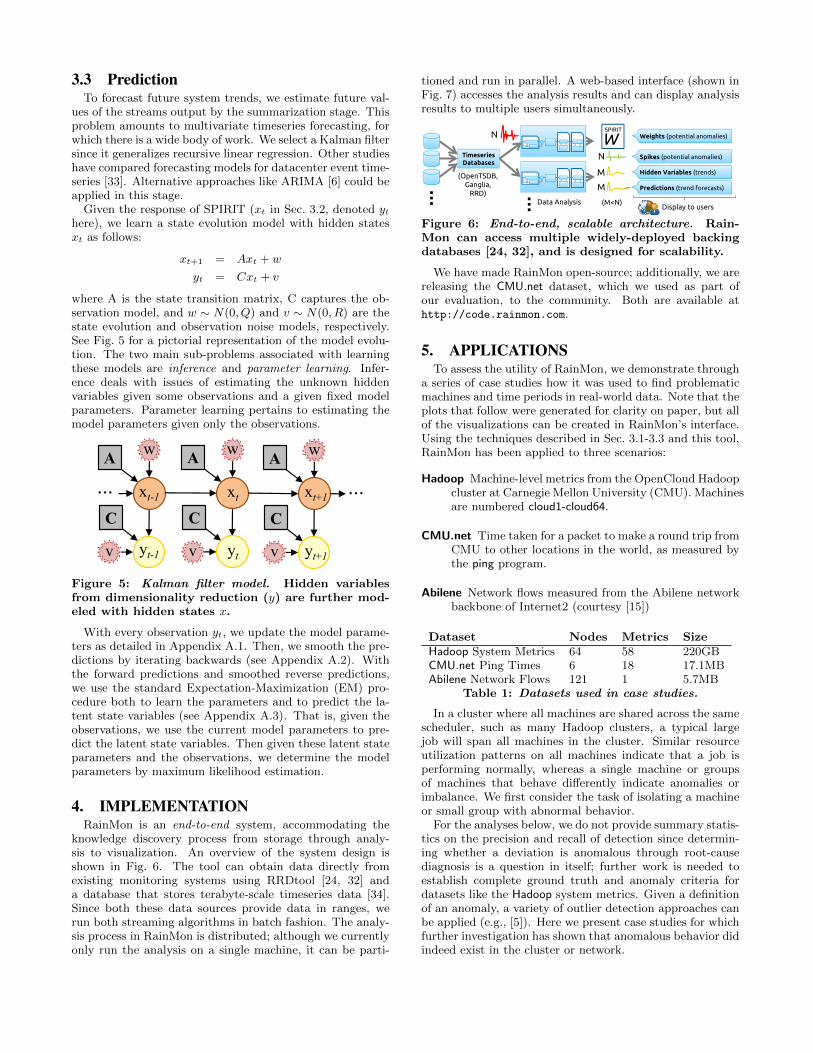
tioned and run in parallel. A web-based interface (shown inFig. 7) accesses the analysis results and can display analysisresults to multiple users simultaneously.

(M<N)

(OpenTSDB,Ganglia,

RRD)Data Analysis

TimeseriesDatabases

N

N

M

M

Hidden Variables (trends)

Weights (potential anomalies)

Spikes (potential anomalies)

Predictions (trend forecasts)

WSPIRIT

Display to users

Figure 6: End-to-end, scalable architecture. Rain-Mon can access multiple widely-deployed backingdatabases [24, 32], and is designed for scalability.

We have made RainMon open-source; additionally, we arereleasing the CMU.net dataset, which we used as part ofour evaluation, to the community. Both are available athttp://code.rainmon.com.

5. APPLICATIONSTo assess the utility of RainMon, we demonstrate through

a series of case studies how it was used to find problematicmachines and time periods in real-world data. Note that theplots that follow were generated for clarity on paper, but allof the visualizations can be created in RainMon’s interface.Using the techniques described in Sec. 3.1-3.3 and this tool,RainMon has been applied to three scenarios:

Hadoop Machine-level metrics from the OpenCloud Hadoopcluster at Carnegie Mellon University (CMU). Machinesare numbered cloud1-cloud64.

CMU.net Time taken for a packet to make a round trip fromCMU to other locations in the world, as measured bythe ping program.

Abilene Network flows measured from the Abilene networkbackbone of Internet2 (courtesy [15])

Dataset Nodes Metrics SizeHadoop System Metrics 64 58 220GBCMU.net Ping Times 6 18 17.1MBAbilene Network Flows 121 1 5.7MB

Table 1: Datasets used in case studies.

In a cluster where all machines are shared across the samescheduler, such as many Hadoop clusters, a typical largejob will span all machines in the cluster. Similar resourceutilization patterns on all machines indicate that a job isperforming normally, whereas a single machine or groupsof machines that behave differently indicate anomalies orimbalance. We first consider the task of isolating a machineor small group with abnormal behavior.

For the analyses below, we do not provide summary statis-tics on the precision and recall of detection since determin-ing whether a deviation is anomalous through root-causediagnosis is a question in itself; further work is needed toestablish complete ground truth and anomaly criteria fordatasets like the Hadoop system metrics. Given a definitionof an anomaly, a variety of outlier detection approaches canbe applied (e.g., [5]). Here we present case studies for whichfurther investigation has shown that anomalous behavior didindeed exist in the cluster or network.

Figure 7: RainMon interface. Overlaid in black boxes is the workflow of the tool. At bottom are the scatterplotof W:,2 vs W:,1 and a machine “energy” heatmap. In the central pane are linked, zoomable, customizabletimeseries plots. An interactive demonstration of the interface is available at http://demo.rainmon.com.

5.1 Outlier Machine IsolationCaused by Machine: After selecting a region of data

to analyze ((1) in Fig. 7), a useful visualization for quicklyidentifying machines that do not behave like others is a plotof the projection coefficients of the first two hidden variablesto each smoothed data stream, i.e., W:,2 vs W:,1 of the PCAweight matrix W (from Algorithm 1, (2) in Fig. 7). If diskreads were closely correlated over time on all machines, anddisk writes were also correlated, we would see two clusterson the plot — one for each metric. For example, in the caseshown in Fig. 8, we see that this is the situation for almostall of the machines (points), but that the metrics for onemachine (cloud11) were far from those for the others.

−0.3 −0.2 −0.1W:,1

−0.3−0.2−0.1

0.00.10.20.30.40.5

W:,

2

cloud11cloud1

Read RequestsWrite Requests

Figure 8: Outlier node discovery. RainMon’s scat-terplot of W:,2 vs W:,1 shows that the coefficients ofcloud11 are separated from the other machines.

From this point, the tool provides the ability to easilyconstruct overlaid timeseries plots of multiple metrics ((3)in Fig. 7). An examination of the disk read behavior ofcloud11 compared with two other cluster members is shownin Fig. 9. Observe that during periods of heavy read activityon other machines it was idle (around Oct. 12), and that

the collection process on the machine failed (the flat linefrom Oct. 13 onwards). Additionally, from the spike datawe found that a burst of read activity on cloud11 occurredbefore a burst on most other nodes.

Oct 12 Oct 13 Oct 14 Oct 15Time

050

100150200250300350400450

Dis

kR

ead

Req

uest

s

Other Nodescloud11

Figure 9: Individual machine examination. Afteridentifying candidate outliers, RainMon allows usersto build custom plots and overlay timeseries data.

Caused by Task: As another example of identifying out-lier nodes in a representative cloud workload, we explicitlyintroduced load imbalance to a job running in the Hadoopcluster. The job is an email classification task running on aHadoop-based machine learning framework [2]. Specifically,in the example input dataset, we generated a number ofduplicated emails under a specific newsgroup topic, so thatthe total amount of input data is approximately an order ofmagnitude larger than that of the other topics. This causedthe Mapper processes handling the topic to last longer andconsume more resources than the others, because of the un-even input distribution.

Fig. 10 compares three different ways of visualizing CPU-related metrics of the Mahout workload in RainMon. Thetop graph shows raw user-level CPU usage of a set of ma-

chines that processed the task, and the middle graph showsspikes of this data extracted by decomposition. The bot-tom graph shows the first and second hidden variables com-puted from the set of CPU-related metrics including user-level CPU usage. The injected excessive input was processedby cloud9 and cloud28, increasing their resource usage. Eventhough the outliers are visible in the original data, they con-sist of multiple datapoints and require a threshold to distin-guish from other behavior. In the extracted spike data, eachsingle datapoint greater than zero can be treated as a po-tential anomaly, and general trends can be observed in thehidden variables hv0 and hv1. Note that spikes can alsobe negative, further emphasizing that domain knowledge isimportant to interpret the meaning. For example, a suddenworkload increase may be witnessed by positive CPU spikes,whereas a brief network problem may manifest through neg-ative network spikes.

22:02:00 22:07:00 22:12:00 22:17:00 22:22:00 22:27:00Time

02468

101214

CP

UU

sage

(Use

r) Original Data

cloud9cloud28other nodes

22:02:00 22:07:00 22:12:00 22:17:00 22:22:00 22:27:00Time

−4−2

02468

10

CP

UU

sage

(Use

r) Extracted Spikes

cloud9cloud28other nodes

22:02:00 22:07:00 22:12:00 22:17:00 22:22:00 22:27:00Time

−10−5

05

101520

Valu

e

Hidden Variables

hv0hv1

Figure 10: Separation of trends and spikes. Anoma-lous timeseries spikes caused by overburdened tasksand overall trends are distinguished by RainMon.

5.2 Machine Group DetectionIt is not always the case that a single machine is an out-

lier. In many cases of uneven workload distribution acrossmachines in a cluster, groups of machines may behave dif-ferently. For example, we identified a case with RainMonwhere all machines were reading data as expected, but therewere two groups of writers—only about half the machineswere writing heavily. Fig. 11, the plot of W:,2 against W:,1,illustrates the two groups of machines, which we have high-lighted with gray rectangles. This was caused by a largeHadoop job whose tasks did not generate even output loadsacross machines. Some of those tasks generated more outputdata than other tasks, causing the machines running thesetasks to experience higher disk write traffic. A programmercan fix this problem by partitioning the data more evenlyacross machines.

5.3 Detecting Correlated RoutersTo demonstrate the applicability of RainMon to network

monitoring, as well as within-datacenter monitoring, we ana-lyze the packet flow count in the Abilene network [15]. Abi-lene is a nationwide high-speed data network for researchand higher education. This public dataset was collectedfrom 11 core routers with packet flow data between every

0.0 0.1 0.2 0.3 0.4W:,1

−0.4

−0.2

0.0

0.2

0.4

W:,

2

Read Requests Write Requests

Figure 11: Machine group discovery. From the scat-terplot, RainMon can also identify groups of ma-chines with different behavior.

−0.10 −0.05 0.00 0.05 0.10 0.15 0.20W:,1

−0.4

−0.3

−0.2

−0.1

0.0

0.1

0.2

W:,

2

Router IPLS

(a) Scatterplot of W:,2 vs W:,1

0 500 1000 1500 2000Time (tick)

−0.06

−0.04

−0.02

0.00

0.02

Nor

mal

ized

Pac

kets

(cou

nt)

(b) Timeseries from the circled group in (a)

Figure 12: Correlated anomaly identification. Rain-Mon’s scatterplot illustrates a cluster of nodes andallows visualization of the anomalous streams. Allstreams shown in (b) correspond to a single routernamed “IPLS.”

pair of nodes for a total of 121 packet flow streams. Weanalyzed a week’s worth of data binned at 5 minute inter-vals for a total of 2016 time ticks. Visualizing this data viathe scatterplot of W:,2 vs W:,1 reveals some tightly clusteredstreams (see Fig. 12(a)) that interestingly all correspond topacket flows from a single router named “IPLS.” Examiningin detail the corresponding data streams, this correlation be-tween “IPLS” and other routers becomes quite evident (seeFig. 12(b)) in the abnormal behavior on its part around timetick 400.

5.4 Time Interval Anomaly DetectionIn addition to finding anomalous machines, RainMon can

be useful in detecting anomalous time intervals. The trendsobserved in hidden variables provide an overall picture oftrends in smoothed data and anomalies across a multi-ticktimescale. This can be helpful in finding unusual behaviorin time from inspection of only a single trend.

Dec 31 Jan 05 Jan 10 Jan 15−11.4−11.2−11.0−10.8−10.6−10.4−10.2

Valu

e

Hidden Variable 1

Dec 31 Jan 05 Jan 10 Jan 150.12

0.16

0.20

0.24

PS

UP

ing

(s)

Time0.21

0.22

0.23

0.24

0.25

Qat

arP

ing

(s)

PSUQatar

Figure 13: Trend discovery. Change in ping time be-havior (Qatar) and sustained increase (PSU) foundfrom the first hidden variable. Absolute values onthe “Value” axis should not be interpreted.

When applying the tool to one year of data from theCMU.net dataset, we could rapidly identify changes in a sin-gle ping destination by examining the first hidden variable.Fig. 13 illustrates one of the cases: we observed a suddenpoint change in the trend that was retained after decom-position around Jan. 5, 2012, and an increase starting atapproximately Jan. 10. From inspection of the weight coef-ficients of the first hidden variable, we isolated two unusualbehaviors on two of the links. First, a point increase in pingtime is clearly observable in the PSU timeseries. Second, thechanges towards the end of the time window shown in thefigure helped identify a change in the “normal” ping time toQatar. This time was nearly constant at 0.221 sec beforeJan. 10, and became 0.226 sec in the period after Jan. 15, achange difficult to localize from the traditional display cur-rently used for the data. A network administrator confirmedthat these sustained changes were legitimate and likely occurdue to maintenance by a telecommunications provider.

5.5 CompressionTo further show concretely how decomposition is effective,

we show how RainMon can compress data, since the sum-mary from dimensionality reduction can be projected backinto the space of the original data. That is, by retaininghidden variables st and the weight matrix W , RainMon canstore a lossy version of the timeseries data — but, by keep-ing spike data, it can also maintain potential anomalies withfull fidelity. Since W is adapted over time in Algorithm 1,one would need to store this matrix at multiple points intime. Therefore, for this evaluation, we perform PCA overan interval of time, rather than use incremental PCA, anduse a fixed number of hidden variables.

Fig. 14 shows the total compressed size of the data seg-ment when stored with a combination of hidden variablesand weight matrix (in red) and spike data (black). For com-parison, we show two alternative compression approaches:using dimensionality reduction on the non-decomposed in-put (blue bars) and storing the original data (green line).

8 12 16 24 32 64Number of Hidden Variables

0

100

200

300

400

Siz

e(k

iloby

tes) HVs + W (With Decomposition)

HVs + W (No Decomposition)

Spike

Original (gzip)

Figure 14: Space savings: storing hidden variablesuses less space than the baseline lossless compressionapproach (green “Original” line).

8 12 16 24 32 64Number of Hidden Variables

0.6

0.7

0.8

0.9

1.0

Rec

onst

ruct

ion

Acc

urac

y WithDecomp.

NoDecomp.

Figure 15: Greater accuracy through decomposition:Storing lossless spike data separately provides im-proved accuracy relative to no decomposition.

For fairness, we apply generic (gzip) compression to thedata in all cases, which is a standard baseline approach tostoring timeseries monitoring data [22]. For M = 16 hid-den variables and eleven 56-hour intervals of 118 streamsof disk access data from the Hadoop dataset, the reduced-dimensionality data and spikes together occupy 114± 5KB.This is 26.5% the size of the gzip-compressed original data(430 ± 80KB), and only requires 16KB (14%) of additionalstorage for the sparse, highly-compressible spike data.

Though spike data requires slightly more space, it yieldsbetter accuracy than using non-decomposed input. For thesame data shown in Fig. 14, Fig. 15 shows the reconstruc-tion accuracy of smoothed+spike data (“With Decomp.”)and PCA as run on the original data (“No Decomp.”)—the former has both higher mean accuracy and lower vari-ance1. Additionally, since spikes are stored with full fidelity,anomaly detection and alerting algorithms that require pre-cise values could operate without loss of correctness.

5.6 PredictionWe further consider how effectively the trends captured

in hidden variables can be forecasted. If projected back intothe original space, future machine utilization can be usefulfor synthetic workload generation and short-term capacityplanning [9]. RainMon uses a Kalman filter as describedin Sec. 3.3 to produce adaptive predictions. To provide anindirect comparison to other approaches, we instead force afixed look-ahead and also run vector autoregression (VAR)[23] and trivial last-value prediction (Constant) for the same

1Reconstruction accuracy A is computed as the geometricmean of the coefficient of determination R2 for each time-series; we compare data where A is defined for both models:

A =

(N∏i=1

1−∑Tt=1(yt,i − yt,i)2∑Tt=1(yt,i − yi)2

)1/N

0 100 200 300 400 500 600 700Time Tick

−25

−20

−15

−10

−5

0Va

lue

Hidden Variable 1Kalman Prediction

(a) Hadoop Prediction

0 10 20 30 40 50Mean Squared Error

0.0

0.2

0.4

0.6

0.8

1.0

Cum

ulat

ive

Freq

uenc

y

ConstantVARKalman

(b) Hadoop MSE

0 500 1000 1500 2000Time Tick

−0.4

−0.3

−0.2

−0.1

0.0

0.1

0.2

0.3

Valu

e

Hidden Variable 1Kalman Prediction

(c) Abilene Prediction

0.000 0.005 0.010 0.015 0.020 0.025Mean Squared Error

0.0

0.2

0.4

0.6

0.8

1.0

Cum

ulat

ive

Freq

uenc

y

ConstantVARKalman

(d) Abilene MSE

Figure 16: Kalman filter predictive performance. A Kalman filter model was used to predict summarizedhidden variables two hours into the future. Fig. (a) shows the prediction overlaid on the first hidden variablefor a 5-day slice of memory and disk metrics on the Hadoop dataset; (b) shows a CDF of the mean squarederror between the prediction and data as compared to vector autoregression and simple constant prediction.Figs. (c) and (d) show the same for the Abilene dataset.

look-ahead. As seen in Fig. 16, on a slice of Hadoop data,the Kalman filter slightly outperforms VAR, whereas bothVAR and the Kalman filter have less predictive power thanconstant forecast for the Abilene data. Though further workis needed to fully characterize these datasets, this highlightsthe limitation of RainMon’s model-based predictor on par-ticularly self-similar or difficult data.

6. CONCLUSION AND DISCUSSIONUnderstanding usage and behavior in computing clusters

is a significant and growing management problem. Integrat-ing decomposition, dimensionality reduction, and predictionin an end-to-end system has given us enhanced ability toanalyze monitoring data from real-world systems. RainMonhas enabled exploration of cluster data at the granularity ofthe overall cluster and that of individual nodes, and allowedfor diagnosis of anomalous machines and time periods.

Our experience with RainMon has helped to define itslimitations, and we highlight three directions of ongoingwork here. First, parameter selection is both involved andnecessary given the diversity of datacenter streams, and asbriefly glimpsed in Sec. 5.6 the ability to mine monitoringdata varies across environments. Mining other datasets us-ing similar techniques, or optimizing them for the ones westudy, is an ongoing and future challenge.

Second, understanding how analysis results are interpretedis key to improving their presentation. Initial feedback fromindustry visitors and a few administrators has resulted inchanges to RainMon’s interface, but active deployment ofRainMon on more systems and studies with administratorsand cluster users are needed to enhance its utility.

Third, scaling these techniques to larger systems will re-quire further towards performance tuning. Currently, thedownsampling and slicing capabilities of our storage ap-proach have enabled us to handle large datasets like theHadoop streams. However, robustness at even greater scalesremains to be demonstrated. Larger systems also complicatecollection, aggregation, and fault-tolerance.

7. ACKNOWLEDGEMENTSWe greatly appreciate the CMU network operations team

for enabling the use of RainMon on the CMU.net data andthe assistance of OpenCloud administrators. Feedback fromLei Li, Raja Sambasivan, and the anonymous reviewers wasvery helpful in improving this paper. We thank the membersand companies of the PDL Consortium (including Actifio,

APC, EMC, Emulex, Facebook, Fusion-io, Google, Hewlett-Packard Labs, Hitachi, Intel, Microsoft Research, NEC Lab-oratories, NetApp, Oracle, Panasas, Riverbed, Samsung,Seagate, STEC, Symantec, VMware, and Western Digital)for their interest, insights, feedback, and support. This re-search was sponsored in part by Intel via the Intel Scienceand Technology Center for Cloud Computing (ISTC-CC).Ilari Shafer is supported in part by an NDSEG Fellowship,which is sponsored by the Department of Defense.

8. REFERENCES[1] Apache Hadoop, http://hadoop.apache.org/.

[2] Apache Mahout: Scalable machine learning and datamining, http://mahout.apache.org/.

[3] L. Barroso and U. Holzle. The datacenter as acomputer: An introduction to the design ofwarehouse-scale machines. Morgan & ClaypoolPublishers, San Rafael, CA, 2009.

[4] K. Bhaduri, K. Das, and B. Matthews. Detectingabnormal machine characteristics in cloudinfrastructures. In Proc. ICDMW’11, Vancouver,Canada.

[5] M. Breunig, H. Kriegel, R. Ng, and J. Sander. LOF:identifying density-based local outliers. In Proc.SIGMOD’00, Dallas, Texas. ACM.

[6] P. J. Brockwell and R. A. Davis. Introduction to timeseries and forecasting. Springer-Verlag, 2002.

[7] V. Chandola, A. Banerjee, and V. Kumar. Anomalydetection: A survey. ACM Comput. Surv.,41(3):15:1–15:58, July 2009.

[8] D. Fisher, D. Maltz, A. Greenberg, X. Wang,H. Warncke, G. Robertson, and M. Czerwinski. Usingvisualization to support network and applicationmanagement in a data center. In Proc. INM’08,Orlando, FL.

[9] D. Gmach, J. Rolia, L. Cherkasova, and A. Kemper.Workload analysis and demand prediction ofenterprise data center applications. In Proc.IISWC’07, Boston, MA.

[10] V. Guralnik and J. Srivastava. Event detection fromtime series data. In Proc. KDD’99, San Diego, CA.

[11] S. Hirose, K. Yamanishi, T. Nakata, and R. Fujimaki.Network anomaly detection based on eigen equationcompression. In Proc. KDD’09, Paris, France.

[12] E. Hoke, J. Sun, J. Strunk, G. Ganger, andC. Faloutsos. InteMon: continuous mining of sensor

data in large-scale self-infrastructures. ACM SIGOPSOperating Systems Review, 40(3):38–44, 2006.

[13] IBM Tivoli,http://www.ibm.com/developerworks/tivoli/.

[14] M. P. Kasick, J. Tan, R. Gandhi, and P. Narasimhan.Black-box problem diagnosis in parallel file systems.In Proc. FAST’10, San Jose, CA.

[15] A. Lakhina, M. Crovella, and C. Diot. Diagnosingnetwork-wide traffic anomalies. In Proc.SIGCOMM’04, Portland, OR.

[16] Z. Lan, Z. Zheng, and Y. Li. Toward automatedanomaly identification in large-scale systems. IEEETransactions on Parallel and Distributed Systems,21(2):174 –187, Feb. 2010.

[17] W. Leland, M. Taqqu, W. Willinger, and D. Wilson.On the self-similar nature of Ethernet traffic. In Proc.SIGCOMM’93, San Francisco, CA.

[18] L. Li, C. Liang, J. Liu, S. Nath, A. Terzis, andC. Faloutsos. ThermoCast: A cyber-physicalforecasting model for data centers. In Proc. KDD’11,San Diego, CA.

[19] L. Li, J. McCann, N. Pollard, and C. Faloutsos.DynaMMo: Mining and summarization of coevolvingsequences with missing values. In Proc. KDD’09,Paris, France.

[20] L. Li, B. A. Prakash, and C. Faloutsos. Parsimoniouslinear fingerprinting for time series. In Proc.VLDB’10, Singapore.

[21] J. Lin, E. Keogh, L. Wei, and S. Lonardi. ExperiencingSAX: a novel symbolic representation of time series.Data Min. Knowl. Discov., 15(2):107–144, Oct. 2007.

[22] C. Loboz, S. Smyl, and S. Nath. DataGarage:Warehousing massive performance data on commodityservers. In Proc. VLDB’10, Singapore.

[23] H. Lutkepohl. New Introduction to Multiple TimeSeries Analysis. Springer, 2007.

[24] M. L. Massie, B. N. Chun, and D. E. Culler. Theganglia distributed monitoring system: design,implementation, and experience. Parallel Computing,30(7):817–840, July 2004.

[25] Nagios, http://www.nagios.org.

[26] H. Nguyen, Y. Tan, and X. Gu. PAL:Propagation-aware anomaly localization for cloudhosted distributed applications. In Proc. SLAML’11,Cascais, Portugal.

[27] S. Papadimitriou, J. Sun, and C. Faloutsos. Streamingpattern discovery in multiple time-series. In Proc.VLDB’05, Trondheim, Norway.

[28] D. Patnaik, M. Marwah, R. Sharma, andN. Ramakrishnan. Sustainable operation andmanagement of data center chillers using temporaldata mining. In Proc. KDD’09, Paris, France.

[29] J. G. Proakis and M. Salehi. Fundamentals ofCommunication Systems. Prentice Hall, 2004.

[30] G. Reeves, J. Liu, S. Nath, and F. Zhao. Cypress:Managing massive time series streams with multi-scalecompressed trickles. In Proc. VLDB’09, Lyon, France.

[31] S. Roweis and Z. Ghahramani. A Unifying Review ofLinear Gaussian Models. Neural Computation,11(2):305–345, Feb. 1999.

[32] RRDtool, http://www.mrtg.org/rrdtool/.[33] R. K. Sahoo, A. J. Oliner, I. Rish, M. Gupta, J. E.

Moreira, S. Ma, R. Vilalta, and A. Sivasubramaniam.Critical event prediction for proactive management inlarge-scale computer clusters. In Proc. KDD’03, NewYork, NY.

[34] B. Sigoure. OpenTSDB: The distributed, scalable timeseries database. In Proc. OSCON’11, Portland, OR.

[35] J. Sun, S. Papadimitriou, and C. Faloutsos.Distributed pattern discovery in multiple streams. InProc. PAKDD’06, Singapore.

[36] Zenoss, http://www.zenoss.com/.

[37] Y. Zhu and D. Shasha. Efficient elastic burst detectionin data streams. In Proc. KDD’03, Washington, DC.

APPENDIXA. KALMAN FILTER DETAILS

A.1 PredictionGiven the initial model parameters (µt|t and Pt|t) for the

linear dynamical system and the current observation (yt),we update the model parameters to compute µt+1|t+1 andPt+1|t+1 as follows:

Vt = APt|tAT +Σw

Kt+1 = VtCT (CVtC

T +Σv)−1

µt+1|t+1 = Aµt|t+Kt+1(yt+1−CAµt|t)

Pt+1|t+1 = Vt−VtCT (CVtC

T +Σv)−1CVt

A.2 SmoothingGiven the predictions xt|t and Pt|t from above that were

computed over the past T time samples, we compute thesmoothed predictions using predictions from the future:

Ast = Pt|tA

T (Vt)−1

µst = µt|t+As

t (xst+1−Axt|t)

Pst = Pt|t+As

t (Pst+1−Vt)AsT

t

where µst and P 2t are the smoothed estimates of the model

parameters computed by using the observations in the fu-ture. We start at t = T and go backwards to t = 1. Theseare useful for parameter learning as described next.

A.3 Parameter LearningGiven the forward Kalman filter predictions and the smoothed

reverse predictions we estimate all the model parameters asfollows, where n refers to the EM iteration index:

E[xt] = µst

E[xtxTt−1] = Ps

t AsTt−1+µs

t µsTt−1

E[xtxTt ] = Ps

t +µst µ

sTt

An = (∑T

t=2 E[xtxTt−1)(

∑Tt=1 E[xtx

Tt ])−1

Σnw =

∑Tt=2 E[xtx

Tt ]+AnE[xt−1xT

t−1]AnT

T−1−∑T

t=2 E[xtxt−1]AnT +AnE[xt−1xt]

T−1

Cn = (∑T

t=1 ytE[xTt ])(∑T

t=1 E[xtxTt ])−1

Σnv =

∑Tt=1 yty

Tt +CnE[xtx

Tt ]CnT

T−

ytxsTt CnT +Cnxs

tyTt

T

µn0 = E[xt]

Σn0 = E[xtx

Tt ]−E[xt]E[xt]T