Raman Spectroscopy on Biochar - PoliTO

POLITECNICO DI TORINO

MASTER THESIS

Raman Spectroscopy on Biochar

Author:Jacopo ACQUAFRESCA

Supervisor:Prof. Alberto TAGLIAFERRO

Carbon GroupDepartment of Applied Science and Technology

April 4, 2018

http://www.johnsmith.com

http://www.jamessmith.com

http://researchgroup.university.com

http://department.university.com

ii

POLITECNICO DI TORINO

AbstractNanotechnologies for ICTs

Department of Applied Science and Technology

Raman Spectroscopy on Biochar

by Jacopo ACQUAFRESCA

Raman Spectroscopy is one the most used techniques to study materials and nano-materials. After the technical improvement of the equipment used to perform thespectroscopy in the past thirty years, especially in terms of resolution and filter, ithas estabilished as the principal instrument to evaluate and study carbons. The ap-plications are very wide and with well known results, in particular for what concernscrystalline materials like diamond, graphene and grafite, for which is relatively easyto indentify properties and quality of different samples. The important knowledgeslearned in studying these materials had lead to shift the focus to more complex al-lotropes or coumponds, especially amorphous carbons and carbon nano-fibers. Inthis project, we studied a particular type of amorphous carbon: the Biochar. Biocharcan be made in a lot of different ways, using different precursors (that are basicallykind of woods) and differents amount of time and temperature during the processof pyrolysis. The purpose was to find some patterns in the spectra of this extremelydisordered material and being able to relate them to different physical and chem-ical properties of different samples. The majority of work has being done almostentirely in Politecnico di Torino, only the production of the materials has been donealmost entirely at the UK Biochar Research Centre. The process it was divided insome steps: first we perform spectroscopy to every samples to obtain the spectra.Then, using a Matlab program developed in Politecnico di Torino, we refined thespectra drawing the baseline, normalizing data between each other and fitting theresults with a proper set of functions. Finally we confronted the signals finding somecorrespondance in terms of disorder, mostly due to the evolution of the state of thematerials through different temperatures.

http://faculty.university.com

http://department.university.com

iii

AcknowledgementsThis dissertation presents the cumulative results of more than six months of research.During this time, I was greatly supported by many people who contributed in dif-ferent ways and without whom this work would not have been possible.First andforemost, I would like to thank my supervisor Prof. Alberto Tagliaferro – I have feltprivileged to be her Master student and experience the kindly, friendly, and support-ive supervision. Then, special thanks go to Massimo Rovere. He was my supervi-sor for daily activities and experiments planning.I thank some of my colleagues notonly for the help and association in many projects done in these years but also forthe friendship. I would also like to thank all my friends, Giulia and my family foralways being there to help and support me.

iv

Contents

Abstract ii

Acknowledgements iii

1 Introduction 11.1 How to Study Carbons and Why . . . . . . . . . . . . . . . . . . . . . . 11.2 XPS Spectroscopy . . . . . . . . . . . . . . . . . . . . . . . . . . . . . . . 31.3 EELS . . . . . . . . . . . . . . . . . . . . . . . . . . . . . . . . . . . . . . 51.4 Infrared Spectroscopy . . . . . . . . . . . . . . . . . . . . . . . . . . . . 6

2 Raman Spectroscopy 92.1 Introduction to Raman Spectroscopy . . . . . . . . . . . . . . . . . . . . 92.2 Theoretical Basis of Incoherent Light Scattering . . . . . . . . . . . . . . 92.3 Classical Treatment of Raman Scattering . . . . . . . . . . . . . . . . . . 112.4 Selection Rule for Fundamental Vibrations . . . . . . . . . . . . . . . . 122.5 Quantum Mechanical Treatment of Raman Scattering . . . . . . . . . . 14

2.5.1 Vibrational Raman Scattering . . . . . . . . . . . . . . . . . . . . 202.5.2 Vibrational Resonance Raman Scattering . . . . . . . . . . . . . 21

2.6 Applications of Raman Spectroscopy . . . . . . . . . . . . . . . . . . . . 252.6.1 Diamond . . . . . . . . . . . . . . . . . . . . . . . . . . . . . . . . 262.6.2 Hexagonal Diamond . . . . . . . . . . . . . . . . . . . . . . . . . 262.6.3 Graphite and Graphene . . . . . . . . . . . . . . . . . . . . . . . 272.6.4 Amorphous Carbons . . . . . . . . . . . . . . . . . . . . . . . . . 312.6.5 Single-Wall Carbon Nanotubes . . . . . . . . . . . . . . . . . . . 312.6.6 Carbon Nanofibers . . . . . . . . . . . . . . . . . . . . . . . . . . 322.6.7 Glassy Carbon . . . . . . . . . . . . . . . . . . . . . . . . . . . . . 33

3 Experiment 353.1 Experiment Material: Biochar . . . . . . . . . . . . . . . . . . . . . . . . 35

3.1.1 General Considerations about the Raman Spectrum of Biochar . 373.2 Micro-Raman Apparatus . . . . . . . . . . . . . . . . . . . . . . . . . . . 373.3 Measurements . . . . . . . . . . . . . . . . . . . . . . . . . . . . . . . . . 403.4 Analysis of the Raw Signals: Intensity and Fluoresce . . . . . . . . . . . 42

4 Treatment of the Signals 464.1 Baseline . . . . . . . . . . . . . . . . . . . . . . . . . . . . . . . . . . . . . 464.2 Normalization . . . . . . . . . . . . . . . . . . . . . . . . . . . . . . . . . 484.3 Fitting . . . . . . . . . . . . . . . . . . . . . . . . . . . . . . . . . . . . . . 48

5 Analysis of Fitted Spectra 505.1 Characteristics of the Fitted Signals . . . . . . . . . . . . . . . . . . . . . 505.2 Comparisons of ID/IG for Different Materials at the Same Temperature 505.3 Comparison of Id/Ig for Different Temperatures for the Same Material 53

v

5.4 Comparisons of the Width of the Components for Different Tempera-tures of the Same Material . . . . . . . . . . . . . . . . . . . . . . . . . . 55

5.5 Final Integrations of the Work . . . . . . . . . . . . . . . . . . . . . . . . 57

6 Conclusions 64

A Physics formulas 66A.1 Terms of polarizability tensor resulting from the Herzberg-Teller cou-

pling simplifications . . . . . . . . . . . . . . . . . . . . . . . . . . . . . 66A.2 Terms of polarizability tensor resulting from the separation of vibra-

tional terms from the electronic terms . . . . . . . . . . . . . . . . . . . 67

B Biochar data 69

Bibliography 80

vi

List of Figures

1.1 Carbon Atom . . . . . . . . . . . . . . . . . . . . . . . . . . . . . . . . . 11.2 Hybridization of carbon . . . . . . . . . . . . . . . . . . . . . . . . . . . 21.3 Adventitious carbon . . . . . . . . . . . . . . . . . . . . . . . . . . . . . 31.4 Graphene XPS spectra . . . . . . . . . . . . . . . . . . . . . . . . . . . . 41.5 D-Value of XPS . . . . . . . . . . . . . . . . . . . . . . . . . . . . . . . . 41.6 EELS Representation . . . . . . . . . . . . . . . . . . . . . . . . . . . . . 51.7 Carbon EELS . . . . . . . . . . . . . . . . . . . . . . . . . . . . . . . . . . 61.8 IR scheme . . . . . . . . . . . . . . . . . . . . . . . . . . . . . . . . . . . 71.9 IR scheme2 . . . . . . . . . . . . . . . . . . . . . . . . . . . . . . . . . . . 81.10 IR interpretation . . . . . . . . . . . . . . . . . . . . . . . . . . . . . . . . 8

2.1 Electromagnetic field . . . . . . . . . . . . . . . . . . . . . . . . . . . . . 102.2 Dipole displacement . . . . . . . . . . . . . . . . . . . . . . . . . . . . . 132.3 Tripole displacement . . . . . . . . . . . . . . . . . . . . . . . . . . . . . 132.4 Tripole displacement . . . . . . . . . . . . . . . . . . . . . . . . . . . . . 142.5 Resonance Level Scattering . . . . . . . . . . . . . . . . . . . . . . . . . 172.6 Herzberg’s electric dipole . . . . . . . . . . . . . . . . . . . . . . . . . . 192.7 Herzberg’s electric dipole 2 . . . . . . . . . . . . . . . . . . . . . . . . . 202.8 Dipole transition in AIV . . . . . . . . . . . . . . . . . . . . . . . . . . . 232.9 Dipole transition in AIV: other case . . . . . . . . . . . . . . . . . . . . . 242.10 Dipole transition in BIV . . . . . . . . . . . . . . . . . . . . . . . . . . . 252.11 Another case of Dipole transition in BIV . . . . . . . . . . . . . . . . . . 252.12 Diamond Lattice . . . . . . . . . . . . . . . . . . . . . . . . . . . . . . . . 262.13 Diamond Spectrum . . . . . . . . . . . . . . . . . . . . . . . . . . . . . . 262.14 Hexagonal Diamond . . . . . . . . . . . . . . . . . . . . . . . . . . . . . 272.15 Graphite lattice structure . . . . . . . . . . . . . . . . . . . . . . . . . . . 272.16 Graphite Phonon Dispersion . . . . . . . . . . . . . . . . . . . . . . . . . 282.17 Graphene Raman Spectrum . . . . . . . . . . . . . . . . . . . . . . . . . 292.18 Phonon processes in Graphite and Graphene . . . . . . . . . . . . . . . 292.19 Edges of Graphene . . . . . . . . . . . . . . . . . . . . . . . . . . . . . . 302.20 Graphene to Graphite . . . . . . . . . . . . . . . . . . . . . . . . . . . . . 312.21 Amorphous Carbons . . . . . . . . . . . . . . . . . . . . . . . . . . . . . 322.22 Carbon Nanotube . . . . . . . . . . . . . . . . . . . . . . . . . . . . . . . 322.23 Carbon Nanotube Raman Spectrum . . . . . . . . . . . . . . . . . . . . 332.24 Carbon Nanofibers . . . . . . . . . . . . . . . . . . . . . . . . . . . . . . 332.25 Carbon Nanofibers Raman Spectrum . . . . . . . . . . . . . . . . . . . . 342.26 Glassy Carbon Raman Spectrum . . . . . . . . . . . . . . . . . . . . . . 34

3.1 Biochar . . . . . . . . . . . . . . . . . . . . . . . . . . . . . . . . . . . . . 353.2 Biochar Raman Spectrum . . . . . . . . . . . . . . . . . . . . . . . . . . 383.3 Second order Raman Peaks . . . . . . . . . . . . . . . . . . . . . . . . . 383.4 Representation of a micro-Raman Apparatus . . . . . . . . . . . . . . . 393.5 Picture of a micro-Raman Apparatus . . . . . . . . . . . . . . . . . . . . 39

vii

3.6 Lasers . . . . . . . . . . . . . . . . . . . . . . . . . . . . . . . . . . . . . . 403.7 Internal picture of a micro-Raman Apparatus . . . . . . . . . . . . . . . 403.8 Comparison between Raman Apparata . . . . . . . . . . . . . . . . . . 423.9 Comparison of Raw Signals . . . . . . . . . . . . . . . . . . . . . . . . . 433.10 Fluorescence . . . . . . . . . . . . . . . . . . . . . . . . . . . . . . . . . . 433.11 Comparison between spectra of WSP . . . . . . . . . . . . . . . . . . . . 443.12 Comparison between spectra of Mischantus . . . . . . . . . . . . . . . . 443.13 Comparison between spectra of RH . . . . . . . . . . . . . . . . . . . . 45

4.1 Example of a linear baseline . . . . . . . . . . . . . . . . . . . . . . . . . 474.2 Gaussian baseline . . . . . . . . . . . . . . . . . . . . . . . . . . . . . . . 474.3 Gaussian baseline . . . . . . . . . . . . . . . . . . . . . . . . . . . . . . . 484.4 Normalized signals . . . . . . . . . . . . . . . . . . . . . . . . . . . . . . 49

5.1 Focus in first order of Biochar . . . . . . . . . . . . . . . . . . . . . . . . 505.2 Focus in second order of Biochar . . . . . . . . . . . . . . . . . . . . . . 515.3 Focus in second order of Biochar . . . . . . . . . . . . . . . . . . . . . . 525.4 Normalized willows spectra . . . . . . . . . . . . . . . . . . . . . . . . . 535.5 Fitted willow spectrum . . . . . . . . . . . . . . . . . . . . . . . . . . . . 545.6 Comparison between spectra of WSP . . . . . . . . . . . . . . . . . . . . 565.7 Comparison between spectra of WSP . . . . . . . . . . . . . . . . . . . . 565.8 Comparison between spectra of WSP . . . . . . . . . . . . . . . . . . . . 565.9 Comparison between spectra of WSP . . . . . . . . . . . . . . . . . . . . 575.10 Comparison of OSR samples at four different temperatures . . . . . . . 585.11 Comparison between OSR 2200 signal and Graphene spectrum . . . . 585.12 OSR 1500 fitted . . . . . . . . . . . . . . . . . . . . . . . . . . . . . . . . 595.13 OSR 2200 fitted . . . . . . . . . . . . . . . . . . . . . . . . . . . . . . . . 605.14 OSR 700 fitted 1st order . . . . . . . . . . . . . . . . . . . . . . . . . . . 615.15 OSR 1500 fitted 1st order . . . . . . . . . . . . . . . . . . . . . . . . . . . 625.16 OSR 2200 fitted 1st order . . . . . . . . . . . . . . . . . . . . . . . . . . . 625.17 Graphite vs OSR 2200 . . . . . . . . . . . . . . . . . . . . . . . . . . . . . 63

B.1 Biochar List . . . . . . . . . . . . . . . . . . . . . . . . . . . . . . . . . . 69

viii

List of Tables

3.1 List of type of Biochar studied . . . . . . . . . . . . . . . . . . . . . . . . 363.2 Characteristics of the produced materials with respect to the heating

temperature . . . . . . . . . . . . . . . . . . . . . . . . . . . . . . . . . . 37

5.1 Library of Gaussian functions used in the fitting . . . . . . . . . . . . . 515.2 Data of the resulting fitted functions for RH 700-626 . . . . . . . . . . . 515.3 Id/Ig for every material heated at 700 C . . . . . . . . . . . . . . . . . . 525.4 Library of Gaussian functions used in the fitting of willow samples . . 545.5 Data of the resulting fitted functions for Willow 750 series 1011/3 . . . 555.6 Id/Ig for every willow sample . . . . . . . . . . . . . . . . . . . . . . . 555.7 Library of Gaussian functions used in the fitting of mischantus samples 555.8 Id/Ig for every mischantus sample . . . . . . . . . . . . . . . . . . . . . 555.9 Data of the resulting fitted functions for OSR 1500 . . . . . . . . . . . . 595.10 Data of the resulting fitted functions for OSR 2200 . . . . . . . . . . . . 60

1

Chapter 1

Introduction

1.1 How to Study Carbons and Why

Carbon is a chemical element, with atomic number 6 and it belongs to group 14 ofthe periodic table.

FIGURE 1.1: The Bohr representation of a 12-Carbon atom

It one of the most interesting, useful and complex elements because it forms alarge variety of compounds, around the number of ten million, more than any othersingle element, and play a primary role in the life of every living being. It can bondswith many other type of atoms, including carbon, and in very different ways (sin-gle bonds, double bonds and even triple bonds), forming usually multiple stablecovalent bonds. Its exceptional behaviour is due mainly to its hybridization fea-tures: carbon has the electron configuration of 1s2 2s2 2p2, this means that carbonwould have 2 unpaired electrons in its p orbitals and that it will only form 2 bonds,but through the mixing of atomic orbitals it can assume planar (sp hybridization),triangular (sp2 hybridization) or even tetrahedral (sp3 hybridization) shape.

Carbons are a broad class of ordered or disordered solid phases composed pri-marily of elemental carbon. Both synthetic and natural materials belong to this

2 Chapter 1. Introduction

FIGURE 1.2: The hybridization of carbon atoms and some examples.At Rigth from up to down: Methane(CH4),Ethyne(C2H2) and Carbon

Dioxide (CO2)

category and amid the most famous and studied materials we found a lot of al-lotropes of pure carbon, for example graphene, graphite, diamond, carbon nan-otubes, fullerenes, glassy carbon and other materials like carbon fibers, amorphoushydrogenated carbon graphene oxide and chars. The fields of applications are virtu-ally unlimited strarting from mechanical and thermal applications, to electronic andphotonic devices. Carbons can be used in the fabrication of smart and high tech-nology materials, in the area harsh environment, energy storage and conversion,biology, medicine and many other applications of the present and the future. Thekey in discovering the properties of a carbon material is studying its chemical com-position and atomic structure. The main method of investigation is spectroscopythat is defined as the study of the interaction of the matter with radiative energy.

In general we can use different type of radiative energy and different kind ofinstrumentation that exploit different physical phenomena to study this kind of ma-terials. The most important and used ones are:

• XPS

• EELS

• IR Spectroscopy

• Raman Spectroscopy

Now we will briefly discuss these techniques and then we’ll focus on Raman Scat-tering

1.2. XPS Spectroscopy 3

1.2 XPS Spectroscopy

X-ray photoelectron spectroscopy (XPS) is a technique suitable for determining theionization potentials of molecules and so it is avaluable help when it takes the ele-mental composition (in terms of atomic percentage) or the quantitative differentia-tion of the same element in different chemical environments, and that peculiarity isvery useful when you study carbon materials. This techique is performed in a UltraHig Vacuum chamber (expensive and slow) irradiating a material with X-rays andacquiring the subsequently emitted photoelectrons. This procedure is very surface-sensitive because the radiation is composed by electrons with energies below 1500eV that interact with the sample in a way that allow only the electrons from the topatomic layers to escape from the surface. Analysing the energyies of the collectedphotoelectrons we can relate them to the the binding energy of the core levels of anatom that depends on the number of electrons that are located in the valence band. Ina few words you can obtain informations abour the chemical state of the moleculeson the surface of a solid sample of any kind, conductor, insulator or semiconductoras long as compatible with the vacuum environment.

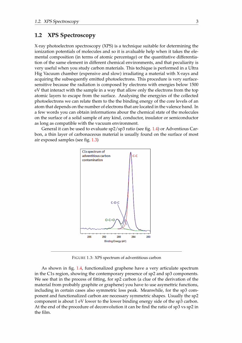
General it can be used to evaluate sp2/sp3 ratio (see fig. 1.4) or Adventious Car-bon, a thin layer of carbonaceous material is usually found on the surface of mostair exposed samples (see fig. 1.3)

FIGURE 1.3: XPS spectrum of adventitious carbon

As shown in fig. 1.4, functionalized graphene have a very articulate spectrumin the C1s region, showing the contemporary presence of sp2 and sp3 components.We see that in the process of fitting, for sp2 carbon (a clue of the derivation of thematerial from probably graphite or graphene) you have to use asymettric functions,including in certain cases also symmetric loss peak. Meanwhile, for the sp3 com-ponent and functionalized carbon are necessary symmetric shapes. Usually the sp2component is about 1 eV lower to the lower binding energy side of the sp3 carbon.At the end of the procedure of deconvolution it can be find the ratio of sp3 vs sp2 inthe film.


FIGURE 1.4: XPS spectra of Graphene Oxide and Graphene

FIGURE 1.5: X-Ray induced C KLL spectra of of a sample of HOPGand Diamond. Right: Grafic scheme of the percentual of sp2 content

in various kind of carbons

Apart from some exceptions like in previous case, it is hard to find a manner to fituniquely mixed sp2/sp3 spectra. If you are studying non functionalized materialsit is more useful focusing on the C KLL Auger peak (a phenomenon stil caused byX-ray irradiation), that is a invaluable method to distinguish sp2 carbon by the sp3component in a semi quantitative way. Shown in fig. 1.5, you can see how it isderived the D-parameter from the differentiated form of the C KLL spectrum. The

1.3. EELS 5

value of that variable is directly linked with the quantity of sp2 and sp3 present in thematerial. This system is instead suitable with more difficulty in the of functionalizedcarbon materials.

1.3 EELS

EELS, or electron energy loss spectroscopy, include all the techniques that study thedifference of energy between electrons sent towards a specimen and the same elec-trons after the interaction with the matter. Also this kind of spectroscopy is veryuseful to determine the chemical properties and the molecular structures of a mate-rial obtaining information about the kind, the number and the chemical state of theatoms and the interactions between them. In the specific of the most important ofthese techniques, trasmission EELS, exploits electrons with kinetic energies from 0.1to 0.3 MeV that penetrate and get through the entire specimen, hitting the detectorbelow. This procedure is performed in a transimission electron microscope (TEM).

FIGURE 1.6: Schematic representation of an electron-sample interac-tion

Among the electrons that arrive at the sample, some of them continue their pathwith unaltered trajectory and energy, some others interact with the materials un-dergo elastic scattering or inelastic scattering (losing energy). This last possibilitylead the specimen to an excited state. The excited state is due to the promotion of acore electron to a higher energy state when it is hitting by an incident electron. Inparticular, it can only get to an empty state of the atoms that can be above the Fermienergy (what we usually mean as the anti bonding orbitals of the molecular orbitaltheory) or even above the vacuum level. TEM detect the energy loss of the scatteredelectrons and correlating that with the energy of the states of the atoms of the stud-ied material find which kind of elements, molecules and bonding is composed thespecimen. There are some applications in the field of carbons: EELS can be usedto detect particles of diamond, fullerene and graphite. This allotropes have similar


absorption peaks because are formed by the same element, usually around 284 eV(obviously due to the electronic states of that element). Fig. 1.7 shows the differ-ences between the EELS spectra of graphite, fullerene and diamond. For example ingraphite we observe a sharp peak that corresponds to excitation of the electron 1sorbital (K shell) to a π anti bonding orbital, that is empty. You can’t find this peak inthe spectrum of diamond because the previously mechanism is impossibile in thatmaterial (there is no π anti bonding orbital).

FIGURE 1.7: EELS spectra of Graphene, Fullerene and Diamond sam-ples

At the end of the day the results and the applications of EELS are very similarto XPS but electron spettroscopy scan a very smaller volume of matter with respectto the X-ray spettroscopy. Another important thing to underline is about the in-strument that performs the EELS. Infact, Trasmission Electron Microscope is a veryexpensive instrument and the sample studied need a specific preparation. The lastimportant thing that it has to be taken in account that generally electrons carry moreenergy to the matter with respect to light rays and there are more probability ofdamaging the sample.

1.4 Infrared Spectroscopy

IR spettroscopy is an analytical technique useful in the study of virtually any kindof material in any physical state. It’s based on incident radiations with wavelenghtcomprise between 4000 and 400 cm-1 (infrared spectrum). Collecting informationsabout the absorption or emission spectrum of a material you can correlate the peaksof the resulting signal directly to the bonds between atoms of the studied mate-rial and then to the elemental composition of the sample[16]. The analysis of thespectrum is not very simple because the interatomic bonds can vibrate in a lot of

1.4. Infrared Spectroscopy 7

different motions (mainly stretching and bending) and may absorb more than oneinfrared frequency. In general stretching produce more relevant peaks than bending,but bending peaks are useful when you have to differentiating types of bonds, likearomatic substitution, that are very similar between each others. The classical the-ory treatment explained the conditions for a material to be infrared active: at leastone of the dipole moment component derivatives with respect to the normal coor-dinate, taken at the equilibrium position, should be non-zero. fig. 1.8 the plot of acomponent of the dipole moment against the normal coordinate that has a gradientdifferent from zero. For example, neither of the carbon-carbon bonds in ethene orethyne absorb IR radiation.

FIGURE 1.8: Dipole moment variations and infrared activities for anA-A and an A-B molecule

Studying accurately the transmitted (or absorbed) spectrum it can be seen themolecular structure of some kind of materials because functional groups give rise tocharacteristic bands both in terms of intensity and position (frequency). For examplecan be used to characterized films of amorphous carbon nitride. fig. 1.10 reveal theposition of some important carbon bonding.


FIGURE 1.9: Dipole moment variations and infrared activities for alinear A-B-A molecule

FIGURE 1.10: Scheme of the interpretation of a IR spectrum

9

Chapter 2

Raman Spectroscopy

2.1 Introduction to Raman Spectroscopy

Raman scattering is one of the most important and used form of molecular spec-troscopy. It’s based on the vibrational transitions of the molecules when irradiatingwith electromagnetic radiation, so Raman spectroscopy is similar to IR spectroscopy,but here are some evident differences between them. First, Raman scattering is a twophoton event meanwhile IR is a one photon event (one photon absorbed and thenone photon emitted). Second, it exploits another property of the matter, the changein the polarizability of the molecule with respect to its vibrational motion. Then aninduced dipole moment arises from the interaction of the polarizability with the in-coming radiation, and this dipole emitted a radiation containing both Rayleigh andRaman scattering. Raman radiation is the light scattering with a shifted frequency ofthe incident radiation due to the loss or the absorption of vibrational energy in themolecule, whereas the Rayleigh radiation is the main peak at the same frequency ofthe light source. The loss of vibrational energy is called anti-Stokes Raman scatter-ing, while if the molecule gains energy we called that phenomenon Stokes Ramanscattering[6].

2.2 Theoretical Basis of Incoherent Light Scattering

For a material, the origin of a scattered radiation are the oscillating electric and mag-netic multipole moments induced by an electromagnetic radiation, in this case a lightray that can be treated in a strictly classical way for both semiclassical and quantumtheories. There are mainly three kinds of source for the multipole moments: the os-cillating electric dipole, the oscillating magnetic dipole and the electric quadrupole.The most intense is the oscillating electric dipole and in most cases is the only phe-nomenon that can be taken in account to evaluate the light scattering because theelectric field can be approximate as constant over a molecule . Chiral systems re-quires the inclusion of the other two terms. The electric dipole radiates a light raywith intensity I:

I = k′ωω4s p2

0 sin2 θ (2.1)

Where p0 is the amplitude of the induced electric dipole with frequency ωs. Themain point for the theorical treatments is to find how ωs and p0 are determined bythe properties of the scattering molecule and the incident electromagnetic radiationof frequency ω1.

One practical way to treat a molecular system in a weak electric field is exploit-ing the perturbation theory for an hamiltonian of a charges system expanding theinteraction system U in a Taylor series in the absence of the field[5].

10 Chapter 2. Raman Spectroscopy

FIGURE 2.1: Illustration of an incoherent light scattering

U[(E)0] = (U)0 + (Eρ)0[∂U

∂(Eρ)0] +

12(Eρ)0(Eσ)0[

∂2U∂(Eρ)0∂(Eσ)0

]

+16(Eρ)0(Eσ)0(Eτ)0[

∂3U∂(Eρ)0∂(Eσ)0∂(Eτ)0

] + . . . (2.2)

In this case it has also known (for hypothesis) that the perturbation is causedinterely by the electric dipole:

U = (U)0 − p0(E0) (2.3)

If we now differentiate eq. (2.2) with respect to E we obtain for the p componentof the total dipole moment, both permanent and induced, of the molecule in thepresence of a static electric field the following result:

pρ = pperρ +

12

αρσ(Eσ)0 +16

βρστ(Eσ)0(Eτ)0 + . . . (2.4)

pper = [∂U

∂(Eρ)0]0 (2.5)

αρσ = [∂2U

∂(Eρ)0∂(Eσ)0] (2.6)

βρστ = [∂3U

∂(Eρ)0∂(Eσ)0∂(Eτ)0] (2.7)

where pperρ is the ρ component of the permanent electric dipole vector pper

ρ and αρσ isa coefficient which relates the σ component of E0 to the ρ component of p.It is evidentthat nine coefficients are required to relate the three components of the vector E0 tothe three components of the vector p. The nine coefficients of αρσ are the componentsof the electric polarizability tensor, a second-rank tensor. Furthermore, βρστ is acoefficient which relates the σ and τ components of E0 to the ρ component of p.Inthe same way of the previous case, 27 such components are needed to relate the ninedyads of the electric field components to the three electric dipole components. The

2.3. Classical Treatment of Raman Scattering 11

twenty-seven coefficients are the components of the third rank tensor, the electrichyperpolarizability tensor βρστ. Using these definitions eq. (2.4) may be written intensor form as:

p = pperρ + α · E +

12

β : E + . . . (2.8)

To simplify we can say:p = pper

ρ + pind (2.9)

pind = p(1) + p(2) + p(3) + . . . (2.10)

p(1) = α · E (2.11)

In the next paragraphs we studied only p(1) that is the dominant terms in the formulaof electric dipole moment and contains the polarizability tensor, the key factor in theRaman Effect.

2.3 Classical Treatment of Raman Scattering

From equation (2.11) we have αρσ that is the and E is the strength of electric field ofthe incident EM wave. For the incident EM wave, the electric field may be expressedas:

E = E0 cos (ω1t) (2.12)

Where ω1 is the angular frequency of the monochromatic EM wave. Instead the po-larizability depends on the relative location of the individual atoms that usually canchange of a little fraction from the equilibrium position. For such small displacementthe variation of the polarizability with vibrations of the molecule can be expressedby expanding each component of the polarizability tensor a in a Taylor series withrespect to the normal coordinates of vibration, as follows:

αρσ = (αρσ)0 + ∑k(

∂αρσ

∂Qk)0Qk +

12 ∑

k,l(

∂2αρσ

∂Qk∂Ql)0QkQl + . . . (2.13)

where (αρσ)0 is the value of αρσ at the equilibrium configuration, Qk Ql . . . are normalcoordinates of vibration associated with the molecular vibrational frequencies ωkωl . . . , and the summations are over all normal coordinates. Then we can truncatethe polynomial to the first two terms and then take in account only one mode ofvibration. So:

αρσ = (αρσ)0 + (∂αρσ

∂Qk)0Qk (2.14)

If we take in account only simple harmonic motion, the time dependence of Qk isgiven by:

Qk = Qk0 cos (ωkt) (2.15)

Where Qk0 is the normal coordinate amplitude. Substituting eq. (2.15) in eq. (2.14)and eq. ( (2.14), (2.12)) in eq. (2.11) we obtain:

p(1) = (αρσ)0E0 cos (ω1t) + (∂αρσ

∂Qk)0E0Qk0 cos (ωkt) cos (ω1t) (2.16)


and then applying trigonometrical substitution:

p(1) = (αρσ)0E0 cos (ω1t) +12(

∂αρσ

∂Qk)0E0Qk0 cos (ω1 + ωk)t

+12(

∂αρσ

∂Qk)0E0Qk0 cos (ω1 −ωk)t (2.17)

then we can name:αRay = (αρσ)0 (2.18)

αRamk =

12(

∂αρσ

∂Qk)0E0Qk0 (2.19)

Eq. (2.17) give you already a lot of informations: you find the three distinct fre-quencies, called ω1, (ω1 −ωk) and (ω1 + ωk), where are created the induced dipolemoments. The first scattered frequency corresponds to the Rayleigh scattering (elas-tic scattering), and it has the same value of the incident frequency, so the conditionis that αRay be non-zero. We know and it is evident that every kind of moleculeis polarizable to a greater or lesser extent, and the classical equilibrium polariz-ability tensor (αρσ)0 will always have some non-zero components and so αRay willbe always non-zero. The results is that all molecules exhibit Rayleigh scattering.The other two frequencies are shifted to higher or lower frequencies and are conse-quently inelastic processes. The scattered light in these two events is called Ramanscattering, with the shorter wavelength shifting (up-shifted frequency) referred to asanti-Stokes scattering, and the longer wavelength shifting (down-shifted frequency)referred to as Stokes scattering. In this cases, the indispensable requirement for Ra-man scattering associated with a molecular frequency ωk is that αRam

k be non-zero.So you need that one of the components of the derived polarizability tensor is non-zero. In general, if we want reassuming, the vibrational displacement of atoms andtherefore a particular vibrational mode lead to a change in polarizability[8].

2.4 Selection Rule for Fundamental Vibrations

Consider a diatomic molecule with maximum vibrational displacement Q0. Whenthe molecule is at maximum extension, the electrons are more readily displaced byan electromagnetic field due to the greater separation causing a lower influence fromthe other atom. Thus the polarizability is increased at the maximum bond length. .In the other case, when it is at maximal compression, the electrons of a given atomfeel the effects of the other atom’s nucleus and hence, they are not perturbed asmuch. Therefore the polarizability is minor for the minimum bond length. Fig. 2.2shows how the behaviour of polarizabily as a function of displacemente near thepoint of equilibrium, for the case of a diatomic molecule. Meanwhile in the case of alinear and non-linear three-atomic molecule, we have a larger number of directionsas shown in fig. 2.3 and fig. 2.4: In general classical theory gives the correct fre-quency dependence for Rayleigh scattering and vibrational Raman scattering. So itleads to good results of equilibrium dipole tensor (αρσ)0 and it can be used to exti-

mate (∂αρσ

∂Qk)0 only in the case of vibrational frequencies of very simple molecules. It

cannot be applied to molecular rotations as classical theory can’t provide the solu-tion for specific discrete rotational frequencies to molecular systems. The results arethat the classical polarizability tensors of the classical treatment can offer only a qual-itative insight to the properties of molecules. In comparison, the quantum transition

2.4. Selection Rule for Fundamental Vibrations 13

FIGURE 2.2: Polarizzability of a diatomic A-B molecule as a functionof vibrational displacement about equilibrium

FIGURE 2.3: Polarizability of a triatomic A-B-A molecule as a functionof vibrational displacement about equilibrium


FIGURE 2.4: Polarizability of a triatomic non-linear A-B-A moleculeas a function of vibrational displacement about equilibrium

polarizability tensors can provide a quantitative understanding about fundamentalmolecular properties and give a much deeper vision of the factors that characterizeRaman scattering. Also the classical amplitude Qk is not very precise and has to bereplaced with a quantum mechanical amplitude.

2.5 Quantum Mechanical Treatment of Raman Scattering

In the quantum mechanical treatment of light-scattering phenomena, we treat theinteracting molecule in the material system quantum mechanically but continue totreat the electromagnetic radiation classically. We shall be concerned in particularwith the allowed transitions between states of the molecule when it is under the per-turbing influence of the incident radiation and the frequency-dependent multipoletransition moments associated with such transitions. The properties of the scatteredradiation can then be determined by regarding such frequency-dependent multi-pole transition moments as classical multipole sources of electromagnetic radiation.In the case of quantum mechanical picture the induced electric dipole of classicaltheory is replaced by the transition electric dipole associated with a transition in themolecule between two states: i, the initial state, and f the final state, that is the resultof the influence on the molecule by the incident electromagnetic radiation of fre-quency ω1 [7]. Hence, we write for the total induced transition electric dipole vectoran equation very similar to eq. 2.10 that was used for the classical treatment:

pindf i = p(1)f i + p(2)f i + p(3)f i + . . . (2.20)

where p(1)f i is linear in E, p(2)f i is quadratic in E, p(3)f i is cubic in E and so on.

2.5. Quantum Mechanical Treatment of Raman Scattering 15

In the same way of the classical treatment we study only the first grade term thattakes this explicit form:

p(1)f i = ( p(1)f i ) + ( p(1)f i )∗ (2.21)

p(1)f i = 〈Ψ(1)f | p|Ψ

(0)i 〉+ 〈Ψ

(0)f | p|Ψ

(1)i 〉 (2.22)

where the Ψ(0)f e Ψ(0)

i are the time-dependent unperturbed wave function of the ini-

tial of the initial and final states of the molecule, the Ψ(1)f and the Ψ(1)

i the perturbedones and p is the electric dipole moment operator. Then, the method for evaluatingeq. 2.22 is as follows. The first thing that we need is the correlation between theperturbed time-dependent wave functions Ψ(1)

i and Ψ(1)f , and the unperturbed time-

dependent wave functions Ψ(1)i and Ψ(0)

f of the system. To find these relationshipswe have to make the following assumptions about the nature of the perturbation:

• First order perturbation

• Interaction hamiltonian for the perturbation is entirely electric dipole in nature

• Perturbation is produced by the time-dependent electric field associated witha plane monochromatic electromagnetic wave of frequency ω1

At this point you can substitute Ψ(1)i and Ψ(1)

f in eq. 2.22. Furthermore, youhave to gather the resulting terms according to their wavelength dependence andidentify the terms which coincide to Rayleigh and Raman radiation. If we wantto preserve generality in the analysis of the incident electromagnetic radiation wemust consider the el. field amplitudes to be complex. On the other hand, for thenext steps of the treatment (to ease the calculations), we take the time-independentwave functions to be real. We need complex wave functions only in a few and rarecases, namely when we have to take in account the magnetic filed or the moleculeshave degenerate states. In general if we apply the quantum mechanics perturbationtheory at the equation following The procedure we have just outlined we obtain forthe ρ component of p(1)f i for real wave functions[2]:

(p(1)ρ ) f i =1

2h ∑r 6=i

{⟨ψ f∣∣ pρ |ψr〉〈ψr| pσ |ψi〉ωri −ω1 − iΓr

Eσ0exp[−i(ω1 −ω f i)t]

+

⟨ψ f∣∣ pρ |ψr〉〈ψr| pσ |ψi〉ωri + ω1 + iΓr

E∗σ0exp[i(ω1 + ω f i)t]}

+1

2h ∑r 6=i

{⟨ψ f∣∣ pσ |ψr〉〈ψr| pρ |ψi〉ωr f −ω1 − iΓr

E∗σ0exp[i(ω1 + ω f i)t]

+

⟨ψ f∣∣ pσ |ψr〉〈ψr| pρ |ψi〉ωr f + ω1 + iΓr

Eσ0exp[−i(ω1 −ω f i)t]}

+ complex conjugate (2.23)

According to Placzek (1934) who call for a theorem made by Klein (1927), the termsin eq. 2.23 involving (ω1 − ω f i) describe the origination of Rayleigh and Ramanscattering provided that (ω1−ω f i) > 0. If ω f i is negative, that is the final state is lessenergetic than the initial state, as in anti-Stokes Raman scattering, this requirementis always satisfied. In the same way, if ω f i is zero, the solution is that the initialand final states have the same energy, and we are talking about Rayleigh scattering,


this requirements is always satisfied. If ω f i is positive, that is the final state is moreenergetic than the initial state, as in Stokes Raman scattering, then the requirementh(ω1 − ω f i) > 0, or equivalently (hω1 > hω f i) > 0 suggests that the energy ofthe irradiating light must be more than sufficient to reach the final state f from theinitial state i. In the case of vibrational or rotational transitions which don’t changethe electronic state, if we take in account frequencies that are in the range of thevisible or the ultraviolet spectrum, this condition is always satisfied. After makingthese assumptions, we can say that the Stokes and anti-Stokes Raman part of the ρcomponent of the real induced transition electric dipole moment can be write in thisway:

(p(1)ρ ) f i =1

2h ∑r 6=i, f

{ 〈 f | pρ |r〉〈r| pσ |i〉ωri −ω1 − iΓr

+〈 f | pσ |r〉〈r| pρ |i〉

ωr f + ω1 + iΓr

}Eσ0exp(−iωst)

+ complex conjugate (2.24)

And knowing the relation between the polarizability tensor and the induced electricdipole from eq. (2.11):

(αρσ) f i =1h ∑

r 6=i, f

{ 〈 f | pρ |r〉〈r| pσ |i〉ωri −ω1 − iΓr

+〈 f | pσ |r〉〈r| pρ |i〉

ωr f + ω1 + iΓr

}(2.25)

The outcomes of the quantum mechanical analysis are generally analogous in formto those obtained from the classical treatment described previously, but instead hav-ing a polarizzability and an oscillating el. dipole, we find a transition electric dipoleand a polarizability tensor.

Unlike the classical polarizability, the quantum mechanical polarizability can de-scribe in theory the properties of the molecules from the informations given from thescattered radiation because is defined in terms of wave functions and energy levelsof the molecules. First, We discuss the frequency denominators (ωri − ω1 − iΓr)which appear in the first term of the transition polarizability (αρσ) f i given by eq.(2.31). In achiving this equation there was no condition that hω1, the energy of aphoton of the incident electromagnetic field, should bear any specific affiliation toany absorption energy hωri of the scattering molecule. Also, no requirements wasmade about the energies of the states |r〉. However, as shown in fig. 2.5 we have intwo main possibilities that can help the calculations: first it is when the frequency ofthe exciting radiation ω1 is very much smaller than any absorption frequency ωri ofthe molecule, that is ωri � ω1 for all r. Then ωri −ω1 ≈ ωri for all states |r〉 and theΓr can be neglected because they are small relative to the ωri. In this case Here thesystem is represented as interacting with incident light of frequency ω1 and makinga transition from an initial stationary state |i〉 to a so-called virtual state and then toa final stationary state | f 〉 with another transition. In particular we noted that thevirtual state which isn’t, as matter of fact, a stationary state of the system. Conse-quently we can say that doesn’t belong to the set of solutions of a time-independentSchrödinger equation and so does not correspond to a well-defined value of the en-ergy. This process, that is a case absorption without energy conservation, give rise tosuch a state is called virtual absorption. When ωri ≈ ω1 the Raman process is illus-trated in fig. 2.5(c) and is called discrete resonance Raman scattering.Meanwhile, ifhω1 is large enough to reach the dissociative continuum energy levels of the systemthe Raman process is illustrated in fig. 2.5(d) and is called continuum resonance Ra-man scattering. Instead, if we focus on the frequency denominator (ω f r + ω1 + iΓr)


in the second term of the transition polarizability (αρσ) f i given by eq. (2.31) we findthat, because is taken in account the sum of ω f r and ω1, this denominator doesn’tbecome small and cannot lead to dominant terms in the sum over r. Consequently,when the first term in (αρσ) f i has one or more dominant terms the other term willbecome relatively unimportant. Now it is very important to point out that the weexpected in the event of resonance Raman scattering a very higher intensity withrespect to normal Raman scattering because, as we know, when ωri ≈ ω1 the firstterm in the formula becomes very small, , but remains large if ωri � ω1. To con-clude, we can say the second term in the expression for (αρσ) f i can be neglected inthe resonance scattering except for stimulated emission which doesn’t concern ushere.

FIGURE 2.5: Four types of Raman Scattering processes

We specified in the introduction to this chapter that we need to introduce somesimplifications to make the general formula for (αρσ) f i more tractable. In this chapterand the subsequent ones we consider these modifications in some detail. Through-out the rest of this chapter we will consider the time-independent wave functionsto be real. The first and fundamental step in solving the more general expressionfor (αρσ) f i given by eq. (2.31) is to apply the adiabatic approximation (from Bornand Oppenheimer, 1927) which enables the electronic and nuclear motions to betreated separately. We expand the notation for a general jth electronic–nuclear stateso that its electronic, vibrational and rotational parts are represented by their respec-tive quantum numbers ej, vj and Rj and write:

|j〉 =∣∣∣ejvjRj

⟩(2.26)


The Born–Oppenheimer, or adiabatic, approximation empower us to set:

|j〉 =∣∣∣ej⟩ ∣∣∣vj

⟩ ∣∣∣Rj⟩

(2.27)

for the state |j〉 and, for its energy,

ωejvjRi = ωej + ωvj + ωRj (2.28)

The general state function is now a product of the discrete electronic, vibrational androtational terms; and the energy is given by the separate electronic, vibrational androtational parts. We now apply the Born–Oppenheimer approximation to eq. (2.31)by introducing equations (2.27) and (2.28). We express the outcome as:

(αρσ)e f v f R f :eivi Ri =⟨

R f∣∣∣ ⟨v f

∣∣∣ ⟨e f∣∣∣ αρσ(er, vr, Rr)

∣∣∣ei⟩ ∣∣∣vi

⟩ ∣∣∣Ri⟩

(2.29)

Now the modifications we can make are effecting closure over the complete set ofrotational states associated with each electronic/vibrational level, and this is pos-sible for most of the practical situations where Raman scattering is observed underexperimental conditions in which the rotational structure is not resolved, and settingei = eg, so assuming that the initial state for the electron is in every case the groundstate, so we assuming that the molecules are fully “relaxed”. So the equation became:

(αρσ)e f v f :egvi =⟨

v f∣∣∣ ⟨e f

∣∣∣ αρσ(er, vr) |eg〉∣∣∣vi⟩

(2.30)

Now we have to consider two different methods. The first one is more radical, weintroduce a number of quite profound approximations, more or less simultaneously,and obtain relatively simple results. This is the method developed by Placzek (1934).The other approach, require the introduction of the approximations in stages. Thisprocedure is particularly precise for the treatment of resonance Raman scatteringand electronic Raman scattering so we will use this second method. From the previ-ous results:

(αρσ)e f v f :egvi =1h ∑

r 6=i, f

{⟨v f∣∣ (pρ)e f er |vr〉〈vr| (pσ)ereg

∣∣vi⟩ωereg + ωvrvi −ω1 − iΓervr

+

⟨v f∣∣ (pσ)e f er |vr〉〈vr| (pρ)ereg

∣∣vi⟩ωereg + ωvrvi + ω1 + iΓervr

}(2.31)

With:(pρ)e f er =

⟨e f∣∣∣ pρ |er〉 (2.32)

(pρ)ereg = 〈er| pρ |eg〉 (2.33)

For these last equations we have to take in account the slight dependence of the elec-tronic transition moments on the normal coordinates of vibration Qk which arisesfrom the dependence of the Hamiltonian of the system itself. This process was firstproposed by Herzberg and Teller (1933) and is called after them. So the electronic


transition dipoles become:

(pρ)e f ′er ′ = (pρ)0e f er +

1h ∑

es 6=er∑

k(pρ)

0e f es

hkeser

ωer −ωesQk

+1h ∑

et 6=e f∑

k(pρ)

0eter

hke f et

ωe f −ωetQk (2.34)

(pσ)er ′eg ′ = (pσ)0ereg +

1h ∑

es 6=er∑

k(pσ)

0eseg

hkeres

ωer −ωesQk

+1h ∑

et 6=eg∑

k(pσ)

0eret

hketeg

ωeg −ωetQk (2.35)

With hkeaeb that is a coupling integral defined in this way:

hkeaeb = 〈ψea(Q0)| (∂He/∂Qk)0 |ψeb(Q0)〉 (2.36)

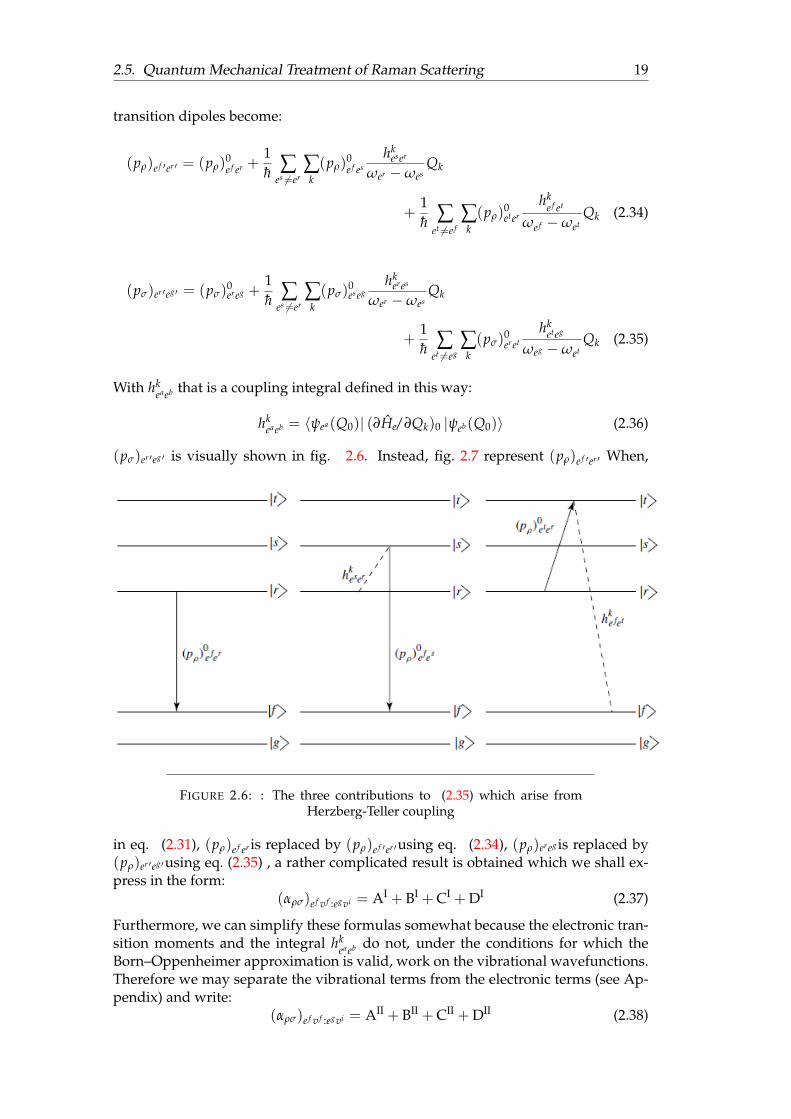
(pσ)er ′eg ′ is visually shown in fig. 2.6. Instead, fig. 2.7 represent (pρ)e f ′er ′ When,

FIGURE 2.6: : The three contributions to (2.35) which arise fromHerzberg-Teller coupling

in eq. (2.31), (pρ)e f er is replaced by (pρ)e f ′er ′using eq. (2.34), (pρ)ereg is replaced by(pρ)er ′eg ′using eq. (2.35) , a rather complicated result is obtained which we shall ex-press in the form:

(αρσ)e f v f :egvi = AI + BI + CI + DI (2.37)

Furthermore, we can simplify these formulas somewhat because the electronic tran-sition moments and the integral hk

eaeb do not, under the conditions for which theBorn–Oppenheimer approximation is valid, work on the vibrational wavefunctions.Therefore we may separate the vibrational terms from the electronic terms (see Ap-pendix) and write:

(αρσ)e f v f :egvi = AII + BII + CII + DII (2.38)


FIGURE 2.7: The three contribution to eq. (2.34) which arise fromHerzberg-Teller coupling

2.5.1 Vibrational Raman Scattering

Further simplifications of eq. (2.38) are possible because we are interested only inpure vibrational Raman scattering for our purposes and equipment because Elec-tronic Raman Scattering is prominent at very low frequencies (is difficult to dividefrom Rayleigh signal). So in our case e f = eg, and we can distinguish two prem-inent situations if we make specific assumptions regarding the relationship of thevibronic absorption frequencies ωervr :egvi , or equivalently ωereg + ωvrvi , to ω1 the fre-quency of the exciting radiation. . If the frequency of the exciting radiation is wellremoved from any electronic absorption frequencies, that is ωereg + ωvrvi � ω1 forall er and vr we have non-resonance or normal vibrational Raman scattering. Asa consequence, ωereg + ωvrvi − ω1 is insensitive to the ωvrvi and may be substitutedby ωereg − ω1. Also provided ω1 � ωvrv f , ωere f + ωvrv f + ω1 can be substitutedby ωere f + ω1; this last simplification does not require that ωere f � ω1. Further, asωereg − ω1 and ωere f + ω1 are now much larger than the damping factor iΓervr thatin this case may be neglected. An important consequence of these modifications inthe frequency denominators is that closure over the set of vibrational states in eachelectronic state er becomes allowed because the denominators are not vr dependent.As opposed to the resonance case which we consider later, a large number of excitedelectronic states |s〉will contribute to the BII, CII and DII terms of eq. (2.38) throughthe matrix elements of the type hk

eaeb delineated in eq. (2.36). The relative magni-tudes of these contributions cannot be easily estabilished and so it is more realisticin the non-resonance situation to use a less explicit equation than that used in eqs.(2.34) and (2.35). Therefore we can write:

(pρ)e f ′er ′ = (pρ)0e f er + ∑

k(pρ)

ke f er Qk (2.39)

Corresponding relationships for (pσ)e f ′er ′ ,(pρ)er ′eg ′ and (pσ)er ′eg ′ are easily given. Wenow introduce into eq. (2.38) the simplifications we have previously debated: theneglection of ωvrvi , ωvrv f and the iγervr , closure over vibrational states, e f = eg andThe use of equations of the type (2.39) instead of eqs. (2.34) and (2.35). When these


conditions are introduced, eq. (2.38) is replaced by:

(αρσ)v f :vi = AIII + BIII + CIII + DIII (2.40)

With:

AIII =1h ∑

er 6=eg

{(pρ)0

eger(pσ)0ereg

ωereg −ω1+

(pσ)0eger(pρ)0

ereg

ωereg + ω1

}(2.41)

BIII + CIII =1h ∑

er 6=eg∑

k

{(pρ)k

eger(pσ)0ereg + (pρ)0

eger(pσ)kereg

ωereg −ω1

+(pσ)0

eger(pρ)kereg + (pσ)k

eger(pρ)0ereg

ωereg + ω1

}⟨v f∣∣∣Qk

∣∣∣vi⟩

(2.42)

DIII =1h ∑

er 6=eg∑k,k′

{(pρ)k

eger(pσ)k′ereg

ωereg −ω1+

(pσ)k′eger(pρ)k

ereg

ωereg + ω1

}⟨v f∣∣∣QkQk′

∣∣∣vi⟩

(2.43)

2.5.2 Vibrational Resonance Raman Scattering

Instead, if the excitation frequency lies within the contour of an electronic absorp-tion band the approximations employed in the treatment of normal scattering areno longer valid. The dependence of the frequency denominator on the vibrationalquantum numbers cannot be disregarded; the frequency difference ωereg +ωvrvi −ω1is very small and proportional to the damping factor iΓervr and so this factor cannotbe ignored; and the explicit dependence of the first-order term in the Herzberg–Tellerformulation on the excited states |s〉 must be taken into account. Nonetheless, fur-ther simplifications are possible. When ω1 reaches some particular electronic ab-sorption frequency ωereg + ωvrvi , the excited electronic state involved will dominatethe summation over states in the expression for the transition polarizability. It isthen generally adequate to consider one or at most two electronic manifolds in theanalysis of Raman scattering in the case of resonance. Another important thing isthat under resonant conditions, only the first term in each of eqs. AII, BII, CII and DII

can be significant. The second term contributes only a slowly varying backgroundand may be disregarded. Therefore, we can restrict the summation over vibrationalstates to one sum over the states

∣∣∣vr(r)⟩

; and we must contemplate coupling of the

resonant electronic state |er〉 to only one excited electronic state, |es〉 in the BIV termsand

∣∣et⟩ in the CIV terms, and only two excited states |es〉 and∣∣∣es′⟩

where s and s′

could be the same) in the DIV terms. In the same way we can restrict the sum to a sin-gle normal coordinate Qk in the BIV and CIV terms and a pair of normal coordinatesQk and Qk

′ (where k and k′ may be equal) in the DIV term. Results are:

(αρσ)v f :vi = AIV + BIV + CIV + DIV (2.44)

AIV =1h(pρ)

0eger(pσ)

0ereg ∑

vrk

〈v f (g)k |vr(r)

k 〉〈vr(r)k |v

i(g)k 〉

ωervrk :egvi

k−ω1 − iΓervr

k

(2.45)


BIV =1h2 (pρ)

0eges

hkeser

ωer −ωes(pσ)

0ereg ∑

vrk

⟨v f (g)

k

∣∣∣Qk

∣∣∣vr(r)k

⟩〈vr(r)

k |vi(g)k 〉

ωervrk :egvi

k−ω1 − iΓervr

k

+1h2 (pρ)

0eger

hkeres

ωer −ωes(pσ)

0eseg ∑

vrk

〈v f (g)k |vr(r)

k 〉⟨

vr(r)k

∣∣∣Qk

∣∣∣vi(g)k

⟩ωervr

k :egvik−ω1 − iΓervr

k

(2.46)

CIV =1h2

hkeget

ωeg −ωet(pρ)

0eter(pσ)

0ereg ∑

vrk

⟨v f (g)

k

∣∣∣Qk

∣∣∣vr(r)k

⟩〈vr(r)

k |vi(g)k 〉

ωervrk :egvi

k−ω1 − iΓervr

k

+1h2 (pρ)

0eger(pσ)

0eret

hketeg

ωeg −ωet∑vr

k

〈v f (g)k |vr(r)

k 〉⟨

vr(r)k

∣∣∣Qk

∣∣∣vi(g)k

⟩ωervr


k

(2.47)

DIV =1h3 (pρ)

0eges

hkeser hk′

erek′

(ωer −ωes)(ωer −ωes′ )(pσ)

0es′ eg ∑

vrk ,vr

k′

⟨v f (g)

k

∣∣∣Qk

∣∣∣vr(r)k

⟩ ⟨vr(r)

k′

∣∣∣Qk′∣∣∣vi(g)

k′

⟩ωervr


k

(2.48)In these equations the exclusions |er〉 6= |eg〉,|es〉 6= |er〉,

∣∣∣es′⟩6= |er〉 and

∣∣et⟩ 6= |eg〉apply, and an additional sign has been introduced on the vibrational quantum num-bers which appear in the numerators to underline to which electronic state theybelong. Hence, the symbols vki(g) and vk f (g) imply that the initial and final state vibra-tional quantum numbers vki and vk f respectively associate to the ground electronicstate |eg〉. Equally, symbols such as vkr(r) and vkr(s) imply that the intermediate statevibrational quantum number vi

k associate to the intermediate electronic states |er〉and |es〉 respectively with the exclusion that r, s 6= g. The CIV term which is for-mulated in eq. (2.47) involves the vibronic coupling of the ground electronic state|eg〉 to an excited electronic state

∣∣et⟩. In the case of a large energy separation be-tween the ground electronic state and the excited electronic states this term is likelyto be trivial and we shall not consider it further. The DIV term which is delineated ineq. (2.48) relates the vibronic coupling of the excited electronic state |er〉 to two otherexcited electronic states |es〉 and |es ′〉. This term is likely to be very small and willalso not be considered further.

For the AIV term to be non-zero, two conditions must be satisfied. Both thetransition dipole moments (pρ)0

eger and (pσ)0ereg which emerge as a product must be

non-zero; and the multiplication of the vibrational overlap integrals, 〈v f (g)k |vr(r)

k 〉 and

〈vr(r)k |v

i(g)k 〉, must also be non-zero for at least one vr(r)

k value. The first condition isunequivocal. It plainly orders the resonant electronic transition to be electric-dipoleallowed. For strong scattering the transition dipole moments that we are takingin account should have appreciable magnitudes. So the excitation within the con-tour of an intense absorption band, as for example a band arising from a chargetransfer mechanism or a π∗ − π transition, would be favourable.Instead, excitationwithin the contour of a weak band, like one resulting from a ligand-field or spin-forbidden transition, would not be able to generate a considerable AIV term. Wenow examine the second condition, shrinking the discussion to the case of harmonicpotential functions. In the case of orthogonal vibrational wave functions, the vibra-tion overlap integrals , 〈v f (g)

k |vr(r)k 〉 and 〈vr(r)

k |vi(g)k 〉 are zero unless v f (g)

k = vr(r)k and


vr(r)k = vi(g)

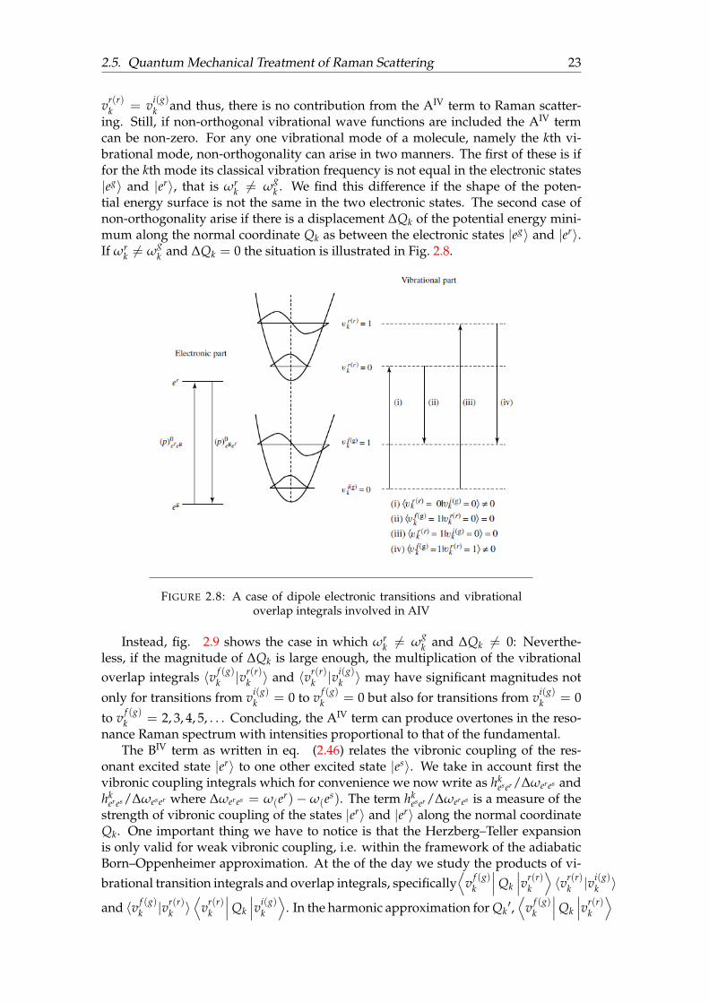
k and thus, there is no contribution from the AIV term to Raman scatter-ing. Still, if non-orthogonal vibrational wave functions are included the AIV termcan be non-zero. For any one vibrational mode of a molecule, namely the kth vi-brational mode, non-orthogonality can arise in two manners. The first of these is iffor the kth mode its classical vibration frequency is not equal in the electronic states|eg〉 and |er〉, that is ωr

k 6= ωgk . We find this difference if the shape of the poten-

tial energy surface is not the same in the two electronic states. The second case ofnon-orthogonality arise if there is a displacement ∆Qk of the potential energy mini-mum along the normal coordinate Qk as between the electronic states |eg〉 and |er〉.If ωr

k 6= ωgk and ∆Qk = 0 the situation is illustrated in Fig. 2.8.

FIGURE 2.8: A case of dipole electronic transitions and vibrationaloverlap integrals involved in AIV

Instead, fig. 2.9 shows the case in which ωrk 6= ω

gk and ∆Qk 6= 0: Neverthe-

less, if the magnitude of ∆Qk is large enough, the multiplication of the vibrationaloverlap integrals 〈v f (g)

k |vr(r)k 〉 and 〈vr(r)

k |vi(g)k 〉 may have significant magnitudes not

only for transitions from vi(g)k = 0 to v f (g)

k = 0 but also for transitions from vi(g)k = 0

to v f (g)k = 2, 3, 4, 5, . . . Concluding, the AIV term can produce overtones in the reso-

nance Raman spectrum with intensities proportional to that of the fundamental.The BIV term as written in eq. (2.46) relates the vibronic coupling of the res-

onant excited state |er〉 to one other excited state |es〉. We take in account first thevibronic coupling integrals which for convenience we now write as hk

eser /∆ωeres andhk

eres /∆ωeser where ∆ωeres = ω(er)− ω(es). The term hkeser /∆ωeres is a measure of the

strength of vibronic coupling of the states |er〉 and |er〉 along the normal coordinateQk. One important thing we have to notice is that the Herzberg–Teller expansionis only valid for weak vibronic coupling, i.e. within the framework of the adiabaticBorn–Oppenheimer approximation. At the of the day we study the products of vi-brational transition integrals and overlap integrals, specifically

⟨v f (g)

k

∣∣∣Qk

∣∣∣vr(r)k

⟩〈vr(r)

k |vi(g)k 〉

and 〈v f (g)k |vr(r)

k 〉⟨

vr(r)k

∣∣∣Qk

∣∣∣vi(g)k

⟩. In the harmonic approximation for Qk

′,⟨

v f (g)k

∣∣∣Qk

∣∣∣vr(r)k

⟩


FIGURE 2.9: A different case of dipole electronic transitions and vi-brational overlap integrals involved in AIV

is non-zero only if v f (g)k = vr(r)

k + 1 and⟨

vr(r)k

∣∣∣Qk

∣∣∣vi(g)k

⟩is non-zero only if vr(r)

k =

vi(g)k + 1. If we consider only diagonal vibrational overlap integrals, that is those for

which vr(r)k = vi(g)

k and v f (g)k = vr(r)

k , the multiplications of the vibrational transi-

tion integrals and overlap integrals are non-zero only if v f (g)k = vr(r)

k + 1. If uppervibrational levels of the kth mode are empty, a case usually described as the lowtemperature limit, then vi(g)

k = 0i(g)k and v f (g)

k = 1 f (g)k so that only two such products

contribute. If we insert the values of the vibrational quantum numbers explicitlyand also give them electronic state sign labels, the two contributing products takethe forms

⟨1 f (g)

k

∣∣∣Qk

∣∣∣0r(r)k

⟩〈0r(r)

k |0i(g)k 〉 and 〈1 f (g)

k |1i(g)k 〉

⟨1r(r)

k

∣∣∣Qk

∣∣∣0i(g)k

⟩. The equa-

tion for BIV term now assumes the following distinct shape which contains onlytwo terms:

αBIV

eg1 fk :eg0i

k=

1h2 (pρ)

0eges

hkeser

∆ωeres(pσ)

0ereg

⟨1 f (g)

k

∣∣∣Qk

∣∣∣0r(r)k

⟩〈0r(r)

k |0i(g)k 〉

ωer0rk :eg0i

k−ω1 − iΓer0r

k

+1h2 (pρ)

0eger

hkeres

∆ωeres(pσ)

0eseg

〈1 f (g)k |1r(r)

k 〉⟨

1r(r)k

∣∣∣Qk

∣∣∣0i(g)k

⟩ωer1r

k :eg0ik−ω1 − iΓer1r

k

(2.49)

The further application of eq. (2.44) inevitably implicate consideration of the sym-metry of the scattering molecule and of its vibrations and you have to apply grouptheory [1]. We can distinguish three important cases: molecules with only one andtotally symmetric mode of vibrations, molecules with a few totally symmetric modeof vibrations and molecules with non-totally simmetric mode of vibrations.

2.6. Applications of Raman Spectroscopy 25

FIGURE 2.10: 0-0 resonant vibronic transition

FIGURE 2.11: 1-0 resonant vibronic transition

2.6 Applications of Raman Spectroscopy

An application that is now assuming considerable importance is the use of vibra-tional Raman spectra solely for the identification of molecular species. Until rela-tively recently Raman spectra could only be obtained from appreciable amounts ofmaterials and these had to be free from fluorescent contaminants. Thus analyticalapplications were very limited. However the situation has now been transformed


completely by quite dramatic advances in the techniques available for exciting, de-tecting and recording Raman spectra. As a result vibrational Raman spectra can nowbe obtained from minute amounts of material in almost any condition or environ-ment. Raman spectra can be obtained from particular points in a sample and it ispossible, for example, to construct maps of the amount of a particular species acrossa surface.

2.6.1 Diamond

Diamond has a characteristic peak at 1332 cm-1 that is the result of the vibration ofits lattice, composed by cell of two units and sp3-sp3 bond (7.02 eV).

FIGURE 2.12: Lattice structure of diamond

FIGURE 2.13: Raman Spectrum of Diamond

2.6.2 Hexagonal Diamond

Lonsdaleite or hexagonal diamond is an allotrope of carbon. It can be found in na-ture only when a meteorite containing graphite strikes the Earth. It has the pecu-liarity of maintaining a hexagonal graphite lattice structure composed by stack of


“chair like” atomic plan staps containing only sp3 sites. The sp3-sp3 bonds are lessenergetic with respect to the pure diamond ones (7.015 eV) and this is reflected oncorresponding Raman spectra that shows the dowshifted value of less then 10 cm-1(=1325 cm-1) for the main D peak[12].

FIGURE 2.14: Lonsdaleite “chair like” lattice structure

2.6.3 Graphite and Graphene

Graphite is with diamond the principal crystalline allotrope of carbon. It has layeredand planar structure The individual layers are called graphene. In each layer, thecarbon atoms are hybridized sp2 and they are arranged in a honeycomb lattice withseparation of 0.142 nm, and the distance between planes is 0.335 nm.

FIGURE 2.15: Graphite lattice structure

The phonon dispersion, of graphene plays a very important role in interpretingtheir Raman spectra. In graphene the unit cell is composed by 2 atoms, consequentlysix phonon dispersion modes as shown in Fig. 2.16 out of which three are acoustic(A) and three are optical (O) phonon modes. In the case of both acoustic and opticalmodes we have out-of plane (Z) phonon mode and the other two are in-plane modes,one longitudinal (L) and the last one transverse (T). Therefore, starting from the


FIGURE 2.16: Graphite Phonon Dispersion

highest energy at the Γ point in the Brillouin zone the various phonon modes arenamed as LO, TO, ZO, LA, TA and ZA as seen in fig. 2.16.

The most interesting phonons are the optical ones in the zone-center (Γ) and zoneedge (K and K′) region, considering they are accessible by Raman spectroscopy. TheΓ point optical phonons are doubly degenerate with E2g symmetry for unperturbedgraphene. The vibrations coincide to the rigid relative dislocation of the A and B sub-lattices. This phonon mode is Raman active and accountable for the Raman G modein graphene. The LO phonon branch in the proximity of the Γ point is not Ramanactive in a one phonon process in defect free graphene, since that it has finite wavevector. Nevertheless, when there are some defects in the lattice, it can be activated.Like the LO phonons near the Γ point, the TO phonon branch in the proximity of thezone edge is accessible by a two-phonon Raman process, which gives rise to the G’(also named 2D) mode.

The most intense attributes in the Raman spectrum of monolayer graphene arethe so-called G band appearing at 1582 cm-1 and the 2D band at about 2700 cm-1using laser radiation at 2.41 eV. Instead, if we have a disordered sample or we’relooking at the edge of a graphene sample, we can also see the so-called disorder-induced D-band (or GeA), at around half of the wavelenght of the 2D band (around1350 cm-1 using laser excitation at 2.41 eV). The G-peak in the first-order Ramanspectrum, coincides to the optical mode vibration of two adjacent carbon atoms ona sp2-hybridized graphene layer. There is a perpendicular stretching of the σ bondsalong the plane generating the Raman G peak, which is one phonon intra-valleyscattering process at the Γ point. The double-resonance (DR) process that seen in thecenter and right side of fig. 2.18 begins with an electron of wave-vector k around K


FIGURE 2.17: Example of a Graphene Raman Spectrum

FIGURE 2.18: Phonon processes in Graphite and Graphene

absorbing a photon of the laser source[9].Then, the electron is inelastically scatteredby a phonon or a defect of wavevector q and energy equal to kinetic energy of thephoton to a site near around the K point, with wavevector k+q.Subsequently, theelectron is then scattered back to a k state, and radiates a photon by recombiningwith a hole at a k point. Instead, if we are talking aboutIn the G’-band (in our caseis called 2D), both processes are inelastic scattering events and two phonons are re-quired. The triple-resonance process can happen by both scattering of electrons andholes and the recombination takes place at the inequivalent K’ point with respect toK point with a photon emission as result. In the case of the D band, the general beliefwas that the two scattering processes consist of one elastic scattering event by defectsof the crystal and one inelastic scattering event by emitting or absorbing a phonon,and consequently the 2D was considered its overtones. Recent studies, [11], shows


that it is implausible the relation with the defects of the crystal but instead the peakis due to the edges of the lattice. It is important focus on edges, because their chiral-ity determines the electronic properties. The edge can be formed by carbon atomsorganized in the zigzag or armchair configuration as shown in Fig. 2.19 . Zigzagedges are made of carbon atoms that all belong to one and the same sublattice, whilethe armchair edges contain carbon atoms from either sublattice. For a zigzag edgethe momentum can only be transferred in a direction dz which does not allow theelectron to return to the original valley in reciprocal space as seen in Fig. 2.19 . There-fore zigzag edges don’t give rise to D peak in Raman spectroscopy. In graphene withdefect free edges, if two edges make an angle of 120°, they should be the same. Incontrast, Coupled Double Resonance Raman scattering conditions are fulfilled on Aedge bonds that are simmetric to in-plane K phonon.

FIGURE 2.19: Raman Double Resonance mechanism at the edges

The most important characteristics of G’ (also called 2D) like position, line widthand intensity depend on the number of layers ‘n’ of the graphene layer, as seen inFig. 2.20. This is due to the evolution of the bands of the mono-layer, bi-layer andfew-layer graphene formations. These features can be used to describe the numberof graphene layers ‘n’ in few layer graphene specimen [4]. The G’ band for 1-LG atroom temperature shows a single Lorentzian or Gaussian feature (symmetric peak).For bilayer graphene with Bernal AB layer stacking, both the electronic and phononbands split into two elements. Four different DR processes can occur in bilayer case.Therefore a Raman spectrum of a bilayer graphene specimen with AB stacking canbe fitted with four Lorentzians or Gaussians. Using group theory method for a 3-LG, the number of permitted Raman peaks in the G’ band become fifteen. The highfrequency side of the G’ band begins to dominate starting from 4-LG to HOPG asseen in Fig. 2.20. The G’ band is a convolution of peaks along the entire kz axis.

The recognition of the number of layers by Raman spectroscopy is well knownonly for graphene specimen with AB Bernal stacking. Instead, if we take the exam-ple of randomly rotation stacking like turbostratic graphite, Raman shows a G’ bandthat is a single Lorentzian or Gaussian as in monolayer graphene but with a largerFull Width Half Maximum and much smaller ratio of IG’ versus IG. This is comingfrom the missing of an interlayer interaction between the graphene planes. Recently,


FIGURE 2.20: The measured G’ band with 2.41 eV laser energy forone, two, three and four layer graphene and HOPG

Intravalley R’ peak with center at around 1625 cm-1 is recognized in randomly pro-duced bilayer graphene due to a rotational-induced intervalley Double Resonancescattering. Its features are due on the mismatch rotation angle and can be used as anoptical label for superlattices in bilayer graphene.

2.6.4 Amorphous Carbons

Amorphous Carbon materials are very versatile and very variegated and their pe-culiar properties depends mainly on the ratio of sp2 (graphite-like) to sp3 (diamondlike) bond. There are many types of sp2 bonded carbons with various degrees ofgraphitic ordering, varying from micro-crystalline graphite to glassy carbon. In gen-eral, an amorphous carbon can display any combination of sp3, sp2 and even sp1sites, with the ulterior possibility of showing some traces of hydrogen and nitrogen[3]. This is shown very clearly in fig. 2.21

2.6.5 Single-Wall Carbon Nanotubes

Carbon nanotubes have exceptional electrical, mechanical, magnetic and even opti-cal properties, which make them a suitable contender for use in various applicationssuch as solar cells, memory devices, conductive composites, hydrogen and energystorages, fuel cells, and super capacitors, but this is only a portion of the possibleuses. They are cylindrical tubes formed by sp2 bonded carbon atoms. A CNT is ba-sically a roll of graphene planar sheet so-called single-wall CNT(SWCNT). They canshows well delineated narrow “G” Raman peaks and a sharp GeA peak correspond-ing to vacancies. For such Raman spectrum, no aliphatic bands are noticed and onlysome weak C5/C7 bands between the G and the GeA peak, suggesting some welldefined armchair type edge on internal edges of vacancies.


FIGURE 2.21: Ternary phase diagram of amorphous carbons. Thethree corners correspond to diamond graphite and hydrocarbons, re-

spectively

FIGURE 2.22: Schematic visualization of a SWCNT

2.6.6 Carbon Nanofibers

Carbon Nanofibers (CNF) are discontinous filaments of disordered material which isknown to contain mainly sp2 hybridized carbons and some traces of sp3 carbon [14].They exibhit a sort broader “D” and “G” bands than for graphene what confirm thedisorder, the existence of vacancies and voids with disordered internal edges GeAband, similar to CNT but broader according to the higher level of disorder in thismaterial. However the G band appears to be somewhat upshifted, the D band is ob-served at the expected and theoretical frequency of around 1330 cm-1. If you take inaccount the precise features of the spectrum, in addition to the main D and G band,we can see some broad DG and GG aliphatic bands, C5/C7 rings band and a Dd


FIGURE 2.23: At left, an image of CNTs (photo taken by SEM). Atright raman spectra of two different CNTs.

band probably due to some disordered diamond phase. CNF can be obtained witha wide variety of methods but in every case you have to use CVD, usually at lowpressure and lower temeperatures wih respect to the fabrication of single wall car-bon nanotubes. The high amount of internal carbon hybridized sp3 in contrast withthe composition of CNT could be obtained by a disordered hexagonal diamondlikeH6 analog to the interfacing material structure between the hexagonal graphene sur-face layers and a diamondlike cubic SiC substrate after high temperature treatment.Thus, the so-labelled Ddisorder band or GeA band is in fact a superposition of adisordered diamond peak (Dd) with a vacancy internal edge GeA band.

FIGURE 2.24: Picture of Carbon Nanofibers

2.6.7 Glassy Carbon

Glassy carbon is another kind of amorphous carbon: brittle and nongraphitizable.The spectrum of this material usually exhibit relatively narrow and well definedmain “D” and “G” bands similar to semiconducting SWCNT. Knowing that glassycarbon is produced with high temperature heating of polymers (between 1000/2000°K),


FIGURE 2.25: Raman Spectrum of Carbon Nanofibers

and that corresponding Raman spectrum is analogous to CNT one, it is generallyconsidered a material made by carbon sp2 clusters. Nevertheless, several glassy car-bon features suggest this model can be perfectioned: higher hardness than graphenicand fullerenic material (in the 10GPa/15GPa range) and elasticity, high diffusionbarrier characteristics although of its porosity and particular Raman up and down-shift of the different Raman peaks and band shifting with precursor material typesand with the annealing temperature. On many glassy carbon Raman spectra we cansee a stress upshifted “G” peak (around 1600/1610cm-1) and a distinct upshifted “Ddiamond” peak (around 1350cm1) (with a stress upshifting of the same magnitudethan the shifting of the “G” peak). This upshifted “D diamond peak” is overlappedto a less intense broader “GeA” band, which is not stress upshifted and in parallelto a ample and soft G2p (“2D”) band.

FIGURE 2.26: Raman Spectrum of Glassy Carbon

35

Chapter 3

Experiment

3.1 Experiment Material: Biochar

FIGURE 3.1: Biochar

Heating biomass in a zero-oxygen environment to temperatures of 250°C or greaterproduce energy-rich gases and liquids, and a black porous solid residue called char-coal, or char. When this char has been made expressly to have an application infavor of the nature biologically sostenible, for instance as a soil improver or to storecarbon, we can name this material biochar.So, BIochar is mostly pure carbon andthe thermal process used to produce biochar is called pyrolysis, and by altering thepyrolysis conditions, it’s possible to change the attributes of the biochar. Usually,higher temperatures of the pyrolysis process mean a smaller quantity of char, but itcould lead to a production of a material carbon more stable. The procedure can takefrom minutes to days and eliminate volatile compounds such as water, methane,hydrogen, and tar, and leaves behind around 20-30% of black mass and powder ofthe original weight. The quality of biochars are determined by various chemicaltraits, despite the fact the peculiarities are interrelated, but they are calculated andexaminated separately. The majority of the attributions correlated with the charcoalquality are derived by studies done in the field of the industry, in particular steel andchemical About the quality of the biochar, better chemical characteristics of charcoal

36 Chapter 3. Experiment

are obtained generally with higher levels of fixed carbon and lower levels of ash andvolatiles. It is connected with high amounts of lignin and low quantities of holocel-luloses and extractives in wood. So, the most important properties of Biochar are:

• • The moisture content: it lowers the calorific or heating value of charcoal.Thus, charcoal fresh from the kiln contains usually less than 1% of moisture,but the moisture content could reach 5-10%, as absorption of moisture fromthe humidity of the air itself is rapid. Moreover, when the hygroscopitity ofcharcoal is increased, the moisture content of charcoal can rise to 15% or evenmore. High quality charcoal has the moisture content of around 5-15% of thegross weight of charcoal. Our moisture is very low.

• • The charcoal’s ash content: it is another very important charcoal’s chemi-cal property that define its quality,it is linked to fixed carbon and varies from0.5% to more than 5% depending on raw materials and on carbonization. Ourbiochars exhibit a very high ash content

• The fixed carbon content: it ranges from a low of about 50% to a high or around95%.

• Volatile matter: it is linked to the amount of fixed carbon and depends stronglyon the carbonization temperature varying from 300 ° C to 1000 ° C. Thus at lowtemperatures (300°C) the content of volatiles is high, at carbonization temper-atures of 500-600°C volatiles are lower, at temperatures of around 1000°C thevolatile content is almost zero and yields is around 25%. In general, the volatilematter in charcoal can vary from a high of 40% or more down to 5% or less.

• Yield: at low temperatures (300°C) the charcoal yield is nearly 50%, at car-bonization temperatures of 500-600°C yields is 30%, at temperatures of around1000°C yields is around 25%.

• Hydrogen and oxygen content.

• Toxic residues

Tab. 3.1 resume the informations about the materials we studied (see Appendix forin-depth data).

Acronym Feedstock Nominal HT(°C) Production

OSR Oil Seed Rape 550, 700, 1500, 2200 Pilot-scale rotaryStraw Pellets kiln pyrolysis unit

MSP Mischantus 550, 700 SameStraw Pellets

WSP Wheat Straw Pellets 550, 700 SameSWP Soft Wood Pellets 550, 700 SameRH Rice Husk 550, 700 SameSS Sewage Sludge 550 SameMischantus 350, 550, 750 SameWillow 350, 550, 750 SamePine 550 SamePKS Palm Kernel Shell 550 Same

TABLE 3.1: List of type of Biochar studied

3.2. Micro-Raman Apparatus 37

Nominal HT 550 700(°C)

Moisture (%wt) 1.5-1.8 1-3.6

Carbon (%wt) 46-85 48-90

Hydrogen (%wt) 1.2-2.7 0.6-1.8

Oxygen (%wt) 2.4-10.6 2-7

BiocharYield (%wt) 21-37 17-32

VolatileMatter (%wt) 7-13 7-16

Ash (%wt) 7-16 7-16

TABLE 3.2: Characteristics of the produced materials with respect tothe heating temperature

3.1.1 General Considerations about the Raman Spectrum of Biochar

The two most important things about biochar’s raman spectrum has to be taken inaccount always are:

• Band broadening is always associated to atomic disorder

• Frequency well-defined Raman peak correspond to a resonance and conse-quently to a ordered material structure

First we have to focused on the first orders peak and bands that are present be-tween 1000 to 1700 cm-1 as shown in fig. 3.2 The profile in this section of the spec-trum resemble very much the features of other types of amorphous carbon, for ex-ample hydrogenated amorphous carbon or carbon nano fibers. G peak due to thevibrational mode of aliphatic sp2-sp2 bonds is somewhat upshifted from 1580 toalmost 1600 meanwhile the so-called D peak is in between the Ddiamond peak at1330 cm-1 and the so-called Ddisorder (or GeA) peak at 1350 cm-1. This is due veryprobably to the sovrapposition of the effects and so revealed both the presence ofcarbon atoms hybridized sp3 and vacancies of internal A edges. But the broadeningis so much extended that we can’t excluded the presence of other effects and internalpeaks for example Gc5 and Gc7 peaks at 1490 cm-1 and 1540 cm-1 generated fromcarbon rings of five and seven atoms[10].

Meanwhile for what concerns the “2D zone” between 2300 cm-1 and 3300 cm-1 in fig 3.2, we see a very broad band that covers three main peaks at 2700, 2910,3170. According to recent studies these peaks arise from seven different processes ofRaman resonance scattering[15] , as shown in fig.. 3.3.

3.2 Micro-Raman Apparatus

A micro-raman apparatus is usually made by these important components: an exci-tation source, notch filters, focusing mirrors, a microscope apparatus, a grating anda detector as shown in fig. as well as a PC and a dedicated software [6]. The processis described below:


FIGURE 3.2: Raman spectrum of a sample of Biochar (SWP700-BX20130410)

FIGURE 3.3: Second order Raman peaks

1. The excitation source, usually a laser source, produce a electromagnetic radia-tion of a very precise frequency

2. The light is amplified and then focused on the sample through mirrors and amicroscope

3. The light is scattered by the sample and come back from the same path

3.2. Micro-Raman Apparatus 39

4. Various filters eliminates unwanted frequencies during the route, for exampleRayleigh peak, “useless” and very intense

5. The grating select and split the right frequencies

6. A Charge Coupled Device detector absorb the radiation and convert it intodigital values

FIGURE 3.4: Schematic Representation of a micro-Raman Apparatus

Our measurements have been taken in a Politecnico Lab with two very similar microraman apparatus. The first Raman apparatus is an old Renishaw model, equippedwith only one Laser source at 514.5 nm, and an “open air” microscope stage. Theother one is a more modern Raman Spectrometer InviaH from Renishaw, equippedwith three different laser source (one “green” at 514.5 nm, one red and one blue) an“enclosed” stage and an updated software.

FIGURE 3.5: The most recent Raman Apparatus in PoliTo


FIGURE 3.6: Three different lasers behind Raman apparatus

FIGURE 3.7: What a Raman apparatus looks like inside and how itworks

3.3 Measurements

Making measurements with a Raman apparatus is a relatively easy process and canbe divide in some distinct steps:

1. Switch on the PC, the Laser source and the spectrograph

3.3. Measurements 41

2. Start the software that controls the instrument

3. Calibrate the instrument using a silicon sample because we know that it hasonly one peak precisely at 520 cm-1

4. Prepare the Biochar sample put less than a cubic centimeter of material powderon the microscopic slide, than compress it to obtain a compact planar structure,easier to visualize and to focus

5. Visualization and focusing of the magnified sample

6. Search of a flat and not too “light” fragment of material

7. Select the mode of acquisition, the number of cycle of acquisitions and thepower of the light ray

8. Start the acquisition of the signals

9. Repeat the process of acquisitions at least another time to have consistent sig-nal and avoid wrong results

10. Take the slide, remove the material, clean the slide

11. Repeat from step 4 to step 9 of the process

The most interesting thing we found in making measurements with the two RamanApparatus was that the results were slightly different even considered the amor-phous nature of the sample and the impossibility of finding the exactly same grainfor the measurements. Even if officially the difference between the two should beonly the more easiness of use and the possibility of using more than one laser for themore recent Raman apparatus, we think that could be some difference in sensibility.fig 3.8 shows clearly the problems that arise when we studied Raman spectra ofbiochar materials taken by different instruments. In this case we have four differentsignals of the exactly same sample (SS30) measured with our two Raman apparata.After the normalization related to G peaks, we see that the signals are consistent ifwe considered the same instrumentation and this is a proof that the instruments arenot broken but we cannot confront them between each others. It seems that the oldRaman (Raman 2 in the picture) tend to flattened and compensate the G peak, re-sulting to a greater ID/IG ratio. We came to the conclusion that we had to use onlyone instrument to make all the measurements. So we decide to use only the more“advanced” and more recent micro Raman apparatus.

At the end of the day these are the characteristics of our measurements and thesettings for InviaH Renishaw Raman Spectrometer:

• Light source: green Argon laser with 514.5 nm of wavelength and 2 µm ofdiameter

• Power of the light source: 5 mW (1%)

• Cycles of acquisitions: 3 (some minutes to complete the processes)

• Exposure time for each acquisition: 10 seconds

• Microscope magnification: 50x

• Range of acquisition: from 400 cm-1 to 3500 cm-1


FIGURE 3.8: Comparison of sensibilities between two Differentmicro-Raman Apparata

3.4 Analysis of the Raw Signals: Intensity and Fluoresce

When you have a Raman raw signal you can check and study few things related tothe intensity and fluorescence of the signal, because we use Raman for qualitativeinformation more than for quantitative Intensity of the signal in Biochar materialsis due generally to . Factors like focus, fluctuations in laser intensity and the orien-tation of the sample relative to the laser beam and Direct comparison of intensityvalues obtained from two separate data collection is a little problematic because weare talking about more of of an instrumental data (with an arbitrary unit) rather thana physical data. the difference in intensity is just an artifact in sample preparationand the concentration of the sample in our case can’t be properly controlled beforemeasurements.

So there isn’t clear correlation between the type of wood from which is derivedthe biochar or the temperature of production and the intensity of the signal A plainexample is showed in fig. 3.9: there are three signals from three different samplesof the same material produced in the exactly same way: the most intense one it wastaken days before the other two signals by two different persons. It’s obvious that theintensity of the two almost equal signals is due to the fact that the signals were takenat distance of few minutes and in the same ways. Furthermore, after the treatmentof the signals we confirmed that all the three signals are pratically indistinguishable.

Fluorescence is instead an important phenomenon in spectroscopy and in our ex-periment considered in general unwanted because is competing with Raman scatter-ing especially at low frequencies because in most cases the emitted light has a lowerenergy than the absorbed radiation. As we know, a laser photon hit a molecule andlooses a specific quantity of energy that allows the molecule to vibrate (this the caseof Stokes scattering). Thus, the scattered photon has less energy and the detectedlight shows a frequency shift. The various frequency shifts associated with differ-ent molecular vibrations generates a spectrum that is peculiar of a specific element

3.4. Analysis of the Raw Signals: Intensity and Fluoresce 43

FIGURE 3.9: Comparison of Raw Signals Between Different Materials

or material. Instead, fluorescence or luminescence emission follows an absorptionprocess. For a better understanding, one can refer to fig. 3.10.

FIGURE 3.10: Comparison between Raman scattering and fluores-cence

Fluorescence derives from the emission of a photon from the lowest vibrationallevel of an excited electronic state, succeeding a direct absorption of the photon andrelaxation of the material from its vibrationally excited level of the electronic stateback to the lowest vibrational level of the electronic state. A fluorescence process


(A) Raw signal of asample of Wsp 550

(B) Raw signal of asample of Wsp 700

FIGURE 3.11: Comparison between spectra of WSP

(A) Raw signal of asample of Mischantus

350

(B) Raw signal of asample of Mischantus

750

FIGURE 3.12: Comparison between spectra of Mischantus

generally requires more than 10-9s. Instead, Raman scattering is completed withina picosecond or less. If the excitation photon does not furnish adequate energy tothe molecule, the necessary transition to give rise to fluorescence will not take place.Nevertheless, if fluorescence is produced, it is often much stronger than the Ramansignal, covering Raman features.

This is typical of organic compounds so, in Biochar materials is a good indicatorof the state of carbonization of the sample. So results confirm this hypothesis: asshown in fig 40 there is a clear difference between signals of Biochars at 550 C vs 700C: at lower temperature the fluorescence is higher. This is more evident compairingsamples with larger differences in temperature for example 350 vs 750 (see fig41).The only material that shows similar fluorescence besides the different value of tem-perature is RH. In particular fluorescence for 750 samples is more emphatized thanthe other materials at the same temperature as seen in fig. 3.13.

3.4. Analysis of the Raw Signals: Intensity and Fluoresce 45

(A) Raw signal of asample of RH 550

(B) Raw signal of asample of RH 700

FIGURE 3.13: Comparison between spectra of RH

46

Chapter 4

Treatment of the Signals

As previously said, raw signals of amorphous carbon materials give fews informa-tions, so it is needed a method to refine the spectra and obtain more maneageablesignals. In PoliTo we developed a complete MatLAB program that in few passagesit can extrapolate a fitted signal. The importance of having a fitted and numericallyexact spectrum is justified by the things that we can find after the fitting of the signal:

• The value of the Id vs Ig ratio

• The values of the width of the peaks or bands

• The evolution of the material with the temperature

• The comparison between different materials

In order to achive these results we have modify the spectrum in some distinctpassages:

1. Modifies the values of the spectra taking in account the quantic detection effi-ciency of the detector

2. Draw the baseline for every signal

3. Normalize the spectra between each others

4. Fitting the signals with an appropriate set of functions

Point one is very easy to satisfies, because we know the QDE of our detector, sothe program will make a simple operation for every “point” taken by the CCD inrelation with the wavelength of the light source. In the next sections we will analyzeone by one the next three steps.

4.1 Baseline

Drawing a baseline for a Biochar’s raman spectrum is a fundamental operation be-cause as we previously said the fluorescence in these kinds of materials is very highand we need to eliminate it in order to being able to fit properly the signal. So wedrawed the baseline after make some proper considerations about the fluorescenceand the spectrum itself. The operation of the baseline itself is done thorugh veryprecise and unskippable passages.

First we have to delineate the range of signal that we want to study. In our case isvirtually the entire spectrum so we can leave it untouched but in certain cases at theboundaries the spectra there can be some strumental alterations. In those situationswe cut away the unnecessary part from the data.

4.1. Baseline 47

Then we have to choose the kind of functions that are going to draw the baseline.In general there are a lot of program, unspecific as Origin or specific as the softwareprovide by Renishaw itself, that use a line or a series of line to draw the baseline.This is not phisically justified by theoretical tractation of fluorescence and the effectson materials spectra. Lorentzian and Gaussian functions represent much better thisphenomenon, as shown in fig. 4.2 After choosing the type of functions, we haveto underline the background of the spectrum where there isn’t presence or sign ofpeaks (see fig.. 4.2). You can also choose manually singular points that will be takenin account by the program during the fitting. Finally, we have to choose the methodof interpolation of the functions: we can use the method of func or fminsearch. Thefirst one is faster but less reliable so we used always the second one.

FIGURE 4.1: Example of a linear baseline

FIGURE 4.2: Example of Gaussian baseline

48 Chapter 4. Treatment of the Signals

FIGURE 4.3: Results of Gaussian baseline

4.2 Normalization

After drawing the baselines for all the spectra we have to normalize the signals be-tween each other because, as we know, the intensities of the spectra are in arbitraryunits and we don’t care about those, but we are interested only in the correlationsbetween the shape of the signals. Since we are primarly interested in studying theID/IG region and 2D region heigth is in a certain way we can choose either the Gpeak or the D peak to normalize the spectra regardless. We chose the G peak andperformed the normalizations with another simple program indipendent from thatone we used for fitting and baseline.

4.3 Fitting

The fitting process has to be done strictly after the baseline drawing but it can bedone indipendently the normalization, knowing that the only differences would bein the evaluation of absolute area of the fitting functions. In general, we made firstthe process of normalization and then we fitted the signals, we find this method assimpler, faster and more practical.

The initial procedure is relatively simple: you have to choose a set of functionsthat the program will manipulate to obtain a fitted signal, composed by the sumof all those functions, that minimize the error with respect to the real signal. Thisis a matematical and precisely a numerical process that doesn’t count any physicalinterpretation. Also, the results can slightly vary from time to time, even for the samespectrum. When you choose for the first time the library of functions it is importantto use a set of a lot of functions to be sure of obtain the best fitting possible. Thenyou find how many functions has been used actually and eliminate the worthlessfunctions. After finding the right number of functions that are needed to properly fitthe signals, we found ourselves in the most critical and arbitrary part of the project.

4.3. Fitting 49

FIGURE 4.4: Example of normalizations on G peak

There are two main ways to prosecute the work and we could use two differentapproaches to comparate the materials:

1. Leave to the software the faculty of finding for each signal the best solutionsand then comparate the components of the fitted solutions for every sample

2. Make some attempts for various samples and materials in order to find a set offunctions that can be the same for every spectrum. Then fitting every samplemaintaining fixed centers for every functions

If the materials don’t show a visible peak shifting the second method could bemore maneageagle and lead to more informations because you have only to careabout heights and widths of the components of the fitted spectrum. So we preferredto use the second method.

50

Chapter 5

Analysis of Fitted Spectra

5.1 Characteristics of the Fitted Signals

The general characteristics of the fitted signal are the same for every materials westudied. D peak and G peak zone is perfectly fitted using four gaussians, two foreach peak as shown in fig. 5.1

FIGURE 5.1: D and G bands of OSR 700

For the 2D zone we fitted with three gaussians (see fig. 5.2), hinting at the prob-able derivation from the three peaks that we find in graphene materials at thosewavelengths.

5.2 Comparisons of ID/IG for Different Materials at the SameTemperature

The first important study and comparation we did it was focused on find if differentwoods from which derived the materials and lead to different properties can havedifferent features in Raman spectra. We decided to make comparation between OSR,SWP, WSP, MSP and RH biochars at 700 C, because they are the only materials atthat precise temperature and they are the materials for which we have the most

5.2. Comparisons of ID/IG for Different Materials at the Same Temperature 51

FIGURE 5.2: Second order zone of the spectrum of OSR 700

complete and detailed datasheet (see Appendix). We used a “fixed center” fittingusing a library with those characteristics:

Acronym of the Peak Center of the Peak (cm-1)

D(1) 1298.4D(2) 1348.7G(1) 1542.7G(2) 1587.9

2D(1) 2695.92D(2) 2936.62D(3) 3154.6

TABLE 5.1: Library of Gaussian functions used in the fitting

A similar kind of library was used in fig. 5.1 and fig. 5.2. One result is shownbelow:

Amplitude Center Width Shape ID/IG(Arb. Un.) (cm-1) (cm-1) 1.26

2.83 1298.4 116.1 Gau0.73 1348.7 47.9 Gau1.98 1542.7 87.1 Gau0.85 1587.9 25.5 Gau1.35 2695.9 170.2 Gau0.66 2936.6 105.9 Gau0.22 3154.6 64.8 Gau

TABLE 5.2: Data of the resulting fitted functions for RH 700-626

52 Chapter 5. Analysis of Fitted Spectra

FIGURE 5.3: RH 700-626

Id/Ig ratio was calculated adding the first two gaussians (D(1) and D(2)) anddividing by the sum of the third and fourth functions (G(1) and G(2)). Looking at fig.5.3 is straigthforward the reason which we used a fixed center fitting: the materialsare so amorphous that it’s not easy to divide the “real” D band from the “real” Gband, also because, as we saw in chapter 4.1, that structure is probably formed bysome others resonance raman scatterings. So the absolute value of Id/Ig can’t giveprecise informations about the material but using a properly set of functions withfixed centers we can at least comparate two separate but very similar raman spectra.

Name Id/Ig Name Id/Ig

MSP 700-10 1.13 RH700-627 1.18OSR 700-828 1.25 RH 700-530 1.15OSR 700-621 1.18 RH 700-701 1.06OSR 700-508 1.12 SWP 700-415 1.10WSP 700-429 1.19 SWP 700-410 1.09WSP 700-513 1.14 SwP 700-424 1.14WSP 700-205 1.25 SWP 700-617 1.16RH 700-626 1.26 SWP 700-823 1.15SWP 700-819 1.13

TABLE 5.3: Id/Ig for every material heated at 700 C

As we see from the list above the Id/Ig ratios for our biochar materials are alwaysaround the value of 1.1. The variations that we found (from a minimun value 1.06to maximum value 1.25) we think they can be due to some factors. These signalpass through the step of acquisition, the drawing of the baseline, the normalization

5.3. Comparison of Id/Ig for Different Temperatures for the Same Material 53

and then the mathematical fitting so some discrepancies are taken in account. Also,we see that the different values of Id/Ig are usually distributed equally for everykind of materials, infact if we would make the mean of the values we would obtainpratically the same results for every material. To conclude we can say there are nodifferences in the spectra of different materials.

5.3 Comparison of Id/Ig for Different Temperatures for theSame Material

After demonstrate that it’s very difficult ricavate differences and peculiarity of dif-ferent Biochar’s samples from their raman spectra we focused in the evolution ofthe raman spectra for the same starting material (same woods) and same fabricationfeatures but different NHT (nominal heat temperature). Mischantus and Willowsamples provided by the University of Edinburgh were suited for this purpose: asseen in Appendix we have three different samples at three different temperatures(350, 550 and 750) for both kind of biochar. We noted from the drawing of the base-line and the subsequent normalization that could be some evidences of an evolutionin the features of the raman spectrum for every biochar material. If we compare thesignals, even without mathematical and analytical instrument, we can roughly esti-mate an increment of the “D peak” with respect to the “G peak”. This is shown infig. 5.4:

FIGURE 5.4: Willows of the series 1011/3

To validate our hypotesis we submit these samples to the same procedure viewedin chapter 6.2. For Willows we used this library of functions:



D(1) 1283.4D(2) 1358.0G(1) 1548.7G(2) 1586.3

2D(1) 2676.02D(2) 2930.22D(3) 3162.0

TABLE 5.4: Library of Gaussian functions used in the fitting of willowsamples

One of the results is shown below (fig. 5.5):

FIGURE 5.5: Fitted willow of the series 1011/3

The general results of ID/IG for every willows samples are shown in the nextlist:

From these results it is clear the slight evolution of the ID/IG ratio with respectto the temperature.

We made the same procedure with Mischantus using another type of library offunctions:

And the Id/Ig ratio of every sample is :Even in this case we see the increasing of Id/Ig ratio with respect to the increas-

ing of NHT. The differences between Mischantus and Willow at the same tempera-ture are mainly due to the differences between the set of functions chosen.

5.4. Comparisons of the Width of the Components for Different Temperatures ofthe Same Material

55

Amplitude Center Width Shape ID/IG(Arb. Un.) (cm-1) (cm-1) 1.29

3.32 1283.4 110.2 Gau2.08 1358.0 60.2 Gau3.16 1548.7 76.9 Gau1.04 1586.3 24.9 Gau1.52 2676.0 129.4 Gau1.80 2930.2 128.1 Gau3.02 3162.0 66.9 Gau

TABLE 5.5: Data of the resulting fitted functions for Willow 750 series1011/3

Willow350 Id/Ig Willow550 Id/Ig Willow750 Id/Ig

1009-171 0.94 1009-171 1.02 1009-171 1.231009-177 0.91 1009-177 1.03 1009-177 1.301011-3 0.78 1011-3 1.04 1011-3 1.29

TABLE 5.6: Id/Ig for every willow sample


D(1) 1283.4D(2) 1358.0G(1) 1527.9G(2) 1582.7

2D(1) 2719.72D(2) 2959.22D(3) 3147.3

TABLE 5.7: Library of Gaussian functions used in the fitting of mis-chantus samples

Mischantus350 Id/Ig Mischantus550 Id/Ig Mischantus750 Id/Ig

1011-9 0.67 1011-9 0.85 1011-9 1.041011-17 0.77 1011-17 0.95 1011-17 1.031011-23 0.76 1011-23 0.90 1011-23 1.21

TABLE 5.8: Id/Ig for every mischantus sample

5.4 Comparisons of the Width of the Components for Differ-ent Temperatures of the Same Material

We found to this point differences in Id/Ig ratios vs nominal heating temperatures.So we thought that could be differences in the materials due mainly to the increasingof the heating temperatures. One practical way to analyse the evolution of similarspectra, for example spectra with fixed center’s fitting functions, as in our case, isfocusing on the width of the peaks. Thus, starting from the solutions of the previouschapter (6.2), we relate the value of the width vs NHT for Mischantus and willow:





5.5. Final Integrations of the Work 57


From these results we can extrapolate neat considerations about Biochars: al-though there isn’t an unequivocal trend in the width of the peaks between 350 and550, if we compare the width of the peaks at 350 with the width of the same peaksat 750 we find always a consistent drop for each kind of peak. The behaviour ofthe widths of the peaks are not so clear when you passed from a heating tempera-ture of 350 to 550 for a few reasons: first one is the biochar is at low temperatures,so it is very hard to distinguish very disordered structures, second one is due to itsrelatively small shift in temperature (only 150 degrees), last one is due to the impos-sibility in finding the same spot for different measurements.

5.5 Final Integrations of the Work

Following the previous intuitions, we tried to complete the work studying the Ra-man Spectra of Biochar at much higher temperature. We expected to see a furthernarrowing of the main peaks, D G and the three peaks around 3000 cm-1, that wecan explain as the crystallization and in particular the graphitization of the sample[13]. So we took some spectra from sample of OSR heated at 1500 C at 2200 C, akind of biochar already studied at 550 C and 700 C in chapter 6.2. Fig. 5.10 showsthe non-fitted results, but the main characteristics of the signals are already prettyevident:


FIGURE 5.10: OSR signals

To make clearer the considerations about these last signals we can make a com-parisons with the spectrum of a sample of graphene, as for example in fig. 5.11:

FIGURE 5.11: Comparison between OSR 2200 signal and Graphenespectrum


The obvious next step involve the fitting of the signals. We find these solutions:

FIGURE 5.12: OSR 1500 fitted

Peak Amplitude Center Width Shape ID/IG(Arb. Un.) (cm-1) (cm-1) 1.12

D(1) 5.19 1345.8 26.6 GauD(2) 7.79 1386.0 105.8 GauG(1) 3.14 1576.7 10.5 GauG(2) 8.46 1584.8 36.7 Gau

0.52 1604.3 12.2 Gau2D(1) 5.95 2692.9 42.1 Gau2D(2) 2.37 2697.3 17.1 Gau

9.77 2787.9 233.9 Gau0.75 2930.2 38.2 Gau0.11 3174.5 22.53 Gau0.38 3230.7 14.29 Gau

TABLE 5.9: Data of the resulting fitted functions for OSR 1500


FIGURE 5.13: OSR 2200 fitted

Peak Amplitude Center Width Shape ID/IG(Arb. Un.) (cm-1) (cm-1) 0.45

D 3.19 1352.8 19.1 Gau7.79 1451.0 139.4 Gau

G(1) 3.14 1580.6 21.3 GauG(2) 8.46 1580.8 8.06 Gau

0.52 1619.9 10.1 Gau5.95 2447.4 25.3 Gau

2D(1) 2.37 2693.7 37.0 Gau2D(2) 9.77 2697.0 191.7 Gau

0.75 2941.4 30.8 Gau0.11 3065.5 12.6 Gau0.38 3233.0 15.5 Gau0.38 3230.7 14.29 Gau

TABLE 5.10: Data of the resulting fitted functions for OSR 2200

The comprehension of the elements of the fitted signal is a little bit different fromthe case of lower temperatures, as we studied in previous paragraphs. At these lev-els of crystallization we can distinguish many more peaks and bands than beforeand so we have to use a larger set of functions, but the gaussians will be narrower.As we see from fig. 5.10 in the range of wavelenght of second order raman scatteringwe see a very high 2D peak, this is typical of graphene and graphite (fig. 5.11), andwe explained the meaning in chapter 3.6.3. Instead, in the range of first order ramanscattering (mainly D and G band) we can notice for OSR1500 a substantial narrow-ing of the peaks and for OSR2200 even a great change for D peak, that become a


single gaussian meanwhile the gaussians that was the second D peak become a sim-ple background between D and G bands. Furthermore, the Id/Ig ratios emerge asincomparable each others. Fig . 5.14, 5.15 and 5.16 illustrate very well the differ-ences between the raman spectra. Finally in fig. 5.14, we see the differences betweena sample of graphite and OSR2200. Although very blurred (this is due to the in-strument) graphite has narrower peaks and a lower D peaks with respect to Biochar.Therefore, OSR2200 still shows traces of its (previous) disordered nature.

FIGURE 5.14: OSR 700 fitted in the 1st order "zone"





FIGURE 5.17: Comparison between graphite and OSR2200 spectra

64

Chapter 6

Conclusions

The analytical study of the Raman spectra of carbons has been an ample, variegatedand discussed scientific field in the past few years. The increasing of the precisionand sensibility of the newest machines that performs this type of spectroscopy andthe increasing of the potential applications for a wide variety of carbon based ma-terials have made the process of raman scattering worth of deep researches. Ourproject had and still continue to have great ambition: find correlations between ra-man spectra and properties of biochars is a challenge that could lead to improve-ment and understanding of the material and the mechanisms of scattering and alsofor raman instrument. During the work we deal with a lot of difficulties due to thenature of the material and in some cases also the lack of technical specifications andinformations about some aspects of the behaviour of the raman spectrometer andtheoretically informations about the Raman scattering in biochars. Our initials hy-pothesis and data on the two micro-Raman apparatus state that there shouldn’t bedifferences in sygnals acquired by the two instruments. Instead, results show a cleardistinction in shape between the Raman spectra, probably due to the different sensi-bility and capacity of focus, so we had to study signals take by one only instrumentto deduce consistent conclusions. Theoretical studies and reaserches about the na-ture of the peaks and the bands of amorphous materials and in particular Biocharsare relatively recents and there is still an opening debate about the classification andthe mechanisms of resonance scatterings. In general we can assume that each ofdiscovered and hypotized photon scattering between the range of wavelenght fromaround 1200 cm-1 to 1600 cm-1, mainly sp3-sp3, sp2-sp2 and A-edges vibrations,could have a small or large impact in the formation of Raman spectrum. Unfortu-nately the singular mechanism in the shape of Biochar spectra is pratically uniden-tifiable due to the large number of scatterings, extreme band broadening. Further-more, the process of fitting, made with our software implemented in MatLab, actsonly in a mathematical way and so we can’t trust in it when we have to make phys-ical assumptions. However,we had also taken in account the intrinsic inconsistencyof amorphous materials produced by pyrolysis heating and the single-point Ramanspectroscopy: we can’t be sure that the signal represents the values of carbonizationsthe chemical composition and the electronic state of the entire material. This is oneof the reason why we analyse more samples produced in similar or even identicalways, and for every sample we took at least two different signals in two differentregions. This give us more confidence and lead to more significant conclusions.At the end of the day, we find no distinguishable differences and peculiarities be-tween Biochars produced with slightly different methods of productions (mostlydifferences in time and contaminants) and different wood derivation. Instead, theNominal Highest Treatment Temperature represent a pretty characterizable featurewhen we study the Raman spectra of Biochars. We can see clear evidence in theevaluation of fluorescence of a sample: at higher temperature the material undergo

Chapter 6. Conclusions 65

to a deeper process of carbonization and crystallization, losing its original organicaspect, therefore we notice a reduction of the photoluminesce in the material. Moreaccurately, we find a clear and coherent path in the evolution of the Raman spec-trum of every Biochar. Evaluating the Id/Ig ratio as the sum of every function in therange of the so-called D band divided by the sum of every function in the range ofthe so-called G band we see a regular and constant increment of this factor betweenthe range of 350 C to 750 C. In parallel we notice a complementar narrowing of thewidth of each component of the spectrum whit the increasing of the temperature ofproduction, even in this case from 350 C to 750 C. Finally, in order to avvalorate oursuppositions, we study the signal of Biochar made at much higher temperatures, forexample 1500 C or 2200 C, and we acknowledge beyond a shadow of a doubt theprogresses of and the evolutions of the Raman spectra of Biochars. The process ofgraphitization and crystallization become a lot more clear and this mean more orderand as a consequence we obtain a more detailed spectrum with more and narrowerpeaks.

66

Appendix A

Physics formulas

A.1 Terms of polarizability tensor resulting from the Herzberg-Teller coupling simplifications

AI =1h ∑

ervr 6=egvi ,e f v f

{⟨v f∣∣ (pρ)0

e f er |vr〉〈vr| (pσ)0ereg

∣∣vi⟩ωervr :egvi −ω1 − iΓervr

+

⟨v f∣∣ (pσ)0

e f er |vr〉〈vr| (pρ)0ereg

∣∣vi⟩ωervr :e f v f + ω1 + iΓervr

}(A.1)

BI =1h2 ∑


{⟨v f∣∣∑es 6=er ∑k(pρ)0

e f eshk

eserωer−ωes

Qk |vr〉〈vr| (pσ)0eres


+

⟨v f∣∣∑es 6=er ∑k(pσ)0

e f eshk

eserωer−ωes

Qk |vr〉〈vr| (pρ)0ereg


}

+1h2 ∑


{⟨v f∣∣ (pρ)0

e f er |vr〉〈vr|∑es 6=er ∑khk

eserωer−ωes

Qk(pσ)0eseg


+

⟨v f∣∣ (pσ)0

e f er |vr〉〈vr|∑es 6=er ∑khk

eserωer−ωes

Qk(pρ)0eseg


}(A.2)

CI =1h2 ∑


{⟨v f∣∣∑et 6=e f ∑k

hke f et

ωe f −ωet

Qk(pρ)0eter |vr〉〈vr| (pσ)0

ereg


+

⟨v f∣∣∑et 6=e f ∑k

hke f et

ωe f −ωet

Qk(pσ)0eter |vr〉〈vr| (pρ)0

ereg


}

+1h2 ∑


{⟨v f∣∣ (pρ)0

e f er |vr〉〈vr|∑et 6=eg ∑k(pσ)0eret

hketeg

ωeg−ωetQk∣∣vi⟩

ωervr :egvi −ω1 − iΓervr

+

⟨v f∣∣ (pσ)0

e f er |vr〉〈vr|∑es 6=er ∑k(pρ)0eret

hketeg

ωeg−ωetQk∣∣vi⟩

ωervr :e f v f + ω1 + iΓervr

}(A.3)

A.2. Terms of polarizability tensor resulting from the separation of vibrationalterms from the electronic terms

67

DI =1h3 ∑


{⟨v f∣∣∑es 6=er ∑k(pρ)0

e f eshk

eserωer−ωes

Qk |vr〉〈vr|∑es′ 6=er ∑k′hk′

er es′

ωer−ωes′

Qk′(pσ)0es′ eg


+

⟨v f∣∣∑es′ 6=er ∑k′(pσ)0

e f es′hk′

es′ erωer−ω

es′Qk′ |vr〉〈vr|∑es 6=er ∑k

hkeres

ωer−ωesQk(pρ)0

eseg


}

(A.4)

A.2 Terms of polarizability tensor resulting from the separa-tion of vibrational terms from the electronic terms

AII =1h ∑


{(pρ)0

e f er(pσ)0ereg

ωervr :egvi −ω1 − iΓervr

+(pσ)0

e f er(pρ)0ereg

ωervr :e f v f + ω1 + iΓervr

}〈v f |vr〉〈vr|vi〉 (A.5)

BII =1h2 ∑

ervr 6=egvi ,e f v f∑

es 6=er∑

k

{(pρ)0

e f es hkeser(pσ)0

eres

(ωer −ωes)(ωervr :egvi −ω1 − iΓervr)

+(pσ)0

e f es hkeser(pρ)0

ereg

(ωer −ωes)(ωervr :e f v f + ω1 + iΓervr)

}⟨v f∣∣∣Qk |vr〉〈vr|vi〉

+1h2 ∑


es 6=er∑

k

{(pρ)0

e f er hkeres(pσ)0

eseg

(ωer −ωes)(ωervr :egvi −ω1 − iΓervr)

+(pρ)0

e f er hkeres(pσ)0

eseg

(ωer −ωes)(ωervr :e f v f + ω1 + iΓervr)

}〈v f |vr〉〈vr|Qk

∣∣∣vi⟩

(A.6)

CII =1h2 ∑


et 6=e f eg∑

k

{hk

e f et(pρ)0eter(pσ)0

ereg

(ωe f −ωet)(ωervr :egvi −ω1 − iΓervr)

+hk

e f et(pσ)0eter(pρ)0

ereg

(ωe f −ωet)(ωervr :e f v f + ω1 + iΓervr)


+1h2 ∑


es 6=er∑

k

{(pρ)0

e f er(pσ)0eret hk

eteg

(ωeg −ωet)(ωervr :egvi −ω1 − iΓervr)

+(pσ)0

e f er(pρ)0eret hk

eteg

(ωeg −ωet)(ωervr :e f v f + ω1 + iΓervr)

}〈v f |vr〉〈vr|Qk

∣∣∣vi⟩

(A.7)

68 Appendix A. Physics formulas

DII =1h3 ∑


eses′ 6=er∑k,k′

{(pρ)0

e f es hkeser hk′

eres′ (pσ)0es′ eg

⟨v f∣∣Qk |vr〉〈vr|Qk′

∣∣vi⟩(ωer −ωes)(ωer −ωes′ )(ωervr :egvi −ω1 − iΓervr)

+(pσ)0

e f es′ hk′hk

es′ er hkeres(pρ)0

eseg

⟨v f∣∣Qk′ |vr〉〈vr|Qk

∣∣vi⟩(ωer −ωes′ )(ωer −ωes)(ωervr :e f v f + ω1 + iΓervr)


(A.8)

69

Appendix B

Biochar data

FIGURE B.1: Biochar list

70 Appendix B. Biochar data

Basic Utility Properties Mean Run-to-Run Variation, SD(n)

Moisture(a) wt% (a.r.) 1.83 0.12 (4)

Ctot wt% (d.b.) 75.41 2.75 (4)

H wt% (d.b.) 2.42 0.30 (4)

O (by difference) wt% (d.b.) 9.24 2.30 (4)

H:Ctot Molar ratio 0.38 0.04 (4)

O:Ctot Molar ratio 0.09 0.03 (4)

Corg wt% (d.b.) tbd tbd

H:Corg Molar ratio tbd tbd

Total ash(a) wt% (d.b.) 12.15 1.00 (4)

Total N wt% (d.b.) 0.78 0.09 (4)

pH [-] 9.77 0.21 (4)

Electric conductivity dS/m 0.82 0.18 (4)

Liming (if pH above 7) % CaCO3 tbd tbd

Biochar C stability(b) % C-basis 94.92 0.65 (4)

Advanced Analysis & Soil Enhancement Properties Mean Run-to-Run

Variation, SD(n)

Mineral N (ammonium & nitrate) mg/kg (d.b) <3 - (4)

Total P(c) wt% (d.b.) 0.19 0.04 (4)

Total K(c) wt% (d.b.) 0.95 0.08 (4)

Available P mg/kg (d.b.) tbd tbd

Volatile Matter(a) wt% (d.b.) 11.62 1.54 (4)

Total Surface Area m2/g (d.b.) 33.6 - (1)

External Surface Area m2/g (d.b.) tbd tbd

Feedstock: Miscanthus Straw Pellets | Production: Pilot-scale rotary kiln pyrolysis unit, nominal peak temperature 550°C

Key features: • Reproducible • Extensively characterised • Readily available

Toxicant Reporting - Total Content Mean Run-to-Run Variation, SD(n)

com

pari

son

vs. r

ecom

men

ded

stan

dard

thre

shol

ds+

IBI EBC(premium)

BQM (high grade)

Germination Inhibition Assay pass/fail tbd tbd

Polycyclic Aromatic Hydrocarbons (EPA16)(d) mg/kg dry wt 0.53 0.28 (4) 6-20 4 20

Dioxin/ Furan (PCDD/ Fs)(e) ng/kg dry wt 2.70 - (1) 9 20 20

Polychlorinated Biphenyls (PCBs)(f) ng/kg dry wt 0.04 - (1) 0.2-0.5 0.2 0.50

As

mod

ified

dry

ash

ing

follo

wed

by

ICP-

OES

mg/kg dry wt 1.35 0.62 (3) 12-100 n/a 10

Cd mg/kg dry wt 0.71 0.97 (3) 1.4-39 1 3

Cr mg/kg dry wt 8.67 3.32 (3) 64-1200 80 15

Co mg/kg dry wt 2.69 2.02 (3) 40-150 n/a n/a

Cu mg/kg dry wt 26.64 37.87 (3) 63-1500 100 40

Pb mg/kg dry wt bdl - (3) 70-500 120 60

Hg mg/kg dry wt bdl - (3) 1-17 1 1

Mo mg/kg dry wt 7.90 6.25 (3) 5-20 n/a 10

Ni mg/kg dry wt 4.95 2.01 (3) 47-600 30 10

Se mg/kg dry wt bdl - (3) 1-36 n/a 5

Zn mg/kg dry wt 63.40 30.35 (3) 200-7000 400 150

Production parameters Mean Run-to-Run Variation, SD(n)

Nominal HTT °C 550 - (1)

Reactor wall temp. °C 550 - (1)

Max. char HTT °C 554 - (1)

Heating rate °C/min 65 - (1)

Kiln residence time min 12 - (1)

Mean time at HTT min 3.9 - (1)

Biochar yield wt% (d.b.) 22.81 1.60 (4)

Pyrolysis liquid yield wt% (d.b.) 41.00 - (1)

Pyrolysis gas yield wt% (d.b.) 34.12 - (1)

Pyrolysis liquid HHV MJ/kg 0.37 - (1)

Pyrolysis gas HHV MJ/kg 9.37 - (1)

Notes: HTT=highest treatment temperature, HHV = higher heating value, tbd = to be defined in next version, bdl. = below detection limit, SD = standard deviation (refers to run-to-run consistency, not analytical error) + available standards related to biochar (IBI = International Biochar Initiative, EBC = European Biochar Standard, BQM = Biochar Quality Mandate), e as TEQ (toxic equivalent) values were bdl, total (tetra to octa chlorinated) dioxin/furan content is reported instead.

(a) TGA, (b) Cross A, Sohi SP (2013), (c) Aqua Regia digestion followed by ICP, (d) Soxhlet extraction (toluene, 6h) determination by GCMS, (e) US EPA 1613, (f) AES O84 (based on US EPA 1668)

Biochar C stability compared to a set of 92 biochar

Standard biochar specification sheet – Version 1.0 | November 2014 MSP550

www.biochar.ac.uk | [email protected]

For full details please go to: http://www.charchive.org/record.php?record_id=97

Appendix B. Biochar data 71


Moisture(a) wt% (a.r.) 2.23 0.06 (2)

Ctot wt% (d.b.) 79.18 0.07 (2)

H wt% (d.b.) 1.26 0.12 (2)






Total ash(a) wt% (d.b.) 11.55 0.17 (2)

Total N wt% (d.b.) 1.03 0.03 (2)

pH [-] 9.72 0.30 (4)





Variation, SD(n)

Mineral N (ammonium & nitrate) mg/kg (d.b.) <3 - (2)

Total P(c) wt% (d.b.) 0.76 0.45 (4)

Total K(c) wt% (d.b.) 2.60 0.75 (4)





Feedstock: Miscanthus Straw Pellets | Production: Pilot-scale rotary kiln pyrolysis unit, nominal peak temperature700°C



com

pari

son

vs. r

ecom

men

ded

stan

dard

thre

shol

ds+

IBI EBC(premium)

BQM (high grade)





As

mod

ified

dry

ash

ing

follo

wed

by

ICP-

OES

mg/kg dry wt 1.60 1.41 (3) 12-100 n/a 10

Cd mg/kg dry wt 4.58 7.67 (3) 1.4-39 1 3

Cr mg/kg dry wt 36.14 9.99 (3) 64-1200 80 15


Cu mg/kg dry wt 5.88 0.79 (3) 63-1500 100 40

Pb mg/kg dry wt bdl - (3) 70-500 120 60


Mo mg/kg dry wt 22.63 14.97 (3) 5-20 n/a 10

Ni mg/kg dry wt 30.40 3.86 (3) 47-600 30 10


Zn mg/kg dry wt 44.53 16.61 (3) 200-7000 400 150




Max. char HTT °C tbd tbd



Mean time at HTT min tbd tbd









Standard biochar specification sheet – Version 1.0 | November 2014 MSP700





Moisture(a) wt% (a.r.) 2.61 0.49 (8)

Ctot wt% (d.b.) 68.85 2.26 (4)

H wt% (d.b.) 1.82 0.22 (4)






Total ash(a) wt% (d.b.) 19.50 2.16 (8)

Total N wt% (d.b.) 1.59 0.22 (4)

pH [-] 9.78 0.47 (4)





Variation, SD(n)


Total P(c) wt% (d.b.) 0.29 0.08 (4)

Total K(c) wt% (d.b.) 2.86 0.26 (4)





Feedstock: Oil Seed Rape Straw Pellets | Production: Pilot-scale rotary kiln pyrolysis unit, nominal peak temp. 550°C



com

pari

son

vs. r

ecom

men

ded

stan

dard

thre

shol

ds+

IBI EBC (premium)

BQM (high grade)





As

mod

ified

dry

ash

ing

follo

wed

by

ICP-

OES

mg/kg dry wt 1.09 0.78 (3) 12-100 n/a 10

Cd mg/kg dry wt 1.76 1.57 (3) 1.4-39 1 3

Cr mg/kg dry wt bdl - (3) 64-1200 80 15


Cu mg/kg dry wt 7.86 2.38 (3) 63-1500 100 40

Pb mg/kg dry wt 17.62 15.99 (3) 70-500 120 60


Mo mg/kg dry wt 1.29 0.34 (3) 5-20 n/a 10

Ni mg/kg dry wt 2.49 0.74 (3) 47-600 30 10


Zn mg/kg dry wt 7.22 2.93 (3) 200-7000 400 150







Mean time at HTT min 5 - (1)


Pyrolysis liquid yield wt% (d.b.) tbd tbd

Pyrolysis gas yield wt% (d.b.) tbd tbd






Standard biochar specification sheet – Version 1.0 | November 2014 OSR550





Moisture(a) wt% (a.r.) 3.63 0.73 (6)

Ctot wt% (d.b.) 67.74 0.86 (5)

H wt% (d.b.) 1.09 0.14 (5)






Total ash(a) wt% (d.b.) 21.92 0.52 (6)

Total N wt% (d.b.) 1.26 0.18 (5)

pH [-] 10.41 0.49 (4)





Variation, SD(n)


Total P(c) wt% (d.b.) 0.258 0.079 (5)

Total K(c) wt% (d.b.) 2.98 0.396 (5)





Feedstock: Oil Seed Rape Straw Pellets | Production: Pilot-scale rotary kiln pyrolysis unit, nominal peak temp. 700°C



com

pari

son

vs. r

ecom

men

ded

stan

dard

thre

shol

ds+

IBI EBC(premium)

BQM (high grade)


Polycyclic Aromatic Hydrocarbons (EPA16)(d) mg/kg dry wt <0.11 - (5) 6-20 4 20



As

mod

ified

dry

ash

ing

follo

wed

by

ICP-

OES

mg/kg dry wt 1.09 0.79 (3) 12-100 n/a 10

Cd mg/kg dry wt 2.98 0.13 (3) 1.4-39 1 3

Cr mg/kg dry wt 4.36 0.95 (3) 64-1200 80 15


Cu mg/kg dry wt 13.78 0.93 (3) 63-1500 100 40

Pb mg/kg dry wt bdl - (3) 70-500 120 60


Mo mg/kg dry wt 1.68 0.14 (3) 5-20 n/a 10

Ni mg/kg dry wt 3.27 0.22 (3) 47-600 30 10


Zn mg/kg dry wt 8.80 0.24 (3) 200-7000 400 150











Pyrolysis liquid HHV MJ/kg tbd tbd

Pyrolysis gas HHV MJ/kg tbd tbd




Standard biochar specification sheet – Version 1.0 | November 2014 OSR700





Moisture(a) wt% (a.r.) 1.54 0.30 (8)

Ctot wt% (d.b.) 48.69 2.37 (5)

H wt% (d.b.) 1.24 0.12 (5)






Total ash(a) wt% (d.b.) 47.93 5.43 (8)

Total N wt% (d.b.) 1.04 0.09 (6)

pH [-] 9.71 0.26 (4)





Variation, SD(n)


Total P(c) wt% (d.b.) 0.10 0.07 (4)

Total K(c) wt% (d.b.) 0.39 0.17 (4)





Feedstock: Rice Husk | Production: Pilot-scale rotary kiln pyrolysis unit, nominal peak temperature 550°C



com

pari

son

vs. r

ecom

men

ded

stan

dard

thre

shol

ds+

IBI EBC(premium)

BQM (high grade)





As

mod

ified

dry

ash

ing

follo

wed

by

ICP-

OES

mg/kg dry wt 0.26 0.46 (3) 12-100 n/a 10

Cd mg/kg dry wt 17.84 3.55 (3) 1.4-39 1 3

Cr mg/kg dry wt 4.99 4.92 (3) 64-1200 80 15


Cu mg/kg dry wt 5.40 0.29 (3) 63-1500 100 40

Pb mg/kg dry wt bdl - (3) 70-500 120 60


Mo mg/kg dry wt 0.64 0.46 (3) 5-20 n/a 10

Ni mg/kg dry wt 3.00 2.29 (3) 47-600 30 10


Zn mg/kg dry wt 23.58 4.44 (3) 200-7000 400 150











Pyrolysis liquid HHV MJ/kg 0 - (1)





Standard biochar specification sheet – Version 1.0 | November 2014 RH550





Moisture(a) wt% (a.r.) 1.49 0.41 (9)

Ctot wt% (d.b.) 47.32 1.82 (4)

H wt% (d.b.) 0.63 0.07 (4)






Total ash(a) wt% (d.b.) 47.93 5.43 (9)

Total N wt% (d.b.) 0.85 0.08 (4)

pH [-] 9.81 0.64 (4)





Variation, SD(n)


Total P(c) wt% (d.b.) 0.16 0.04 (4)

Total K(c) wt% (d.b.) 0.62 0.16 (4)



Total Surface Area m2/g (d.b.) 42 - (1)


Feedstock: Rice Husk | Production: Pilot-scale rotary kiln pyrolysis unit, nominal peak temperature 700°C



com

pari

son

vs. r

ecom

men

ded

stan

dard

thre

shol

ds+

IBI EBC(premium)

BQM (high grade)





As

mod

ified

dry

ash

ing

follo

wed

by

ICP-

OES

mg/kg dry wt bdl - (3) 12-100 n/a 10

Cd mg/kg dry wt 19.97 3.35 (3) 1.4-39 1 3

Cr mg/kg dry wt bdl - (3) 64-1200 80 15


Cu mg/kg dry wt 26.93 30.20 (3) 63-1500 100 40

Pb mg/kg dry wt bdl - (3) 70-500 120 60


Mo mg/kg dry wt 0.67 0.19 (3) 5-20 n/a 10

Ni mg/kg dry wt 2.71 0.42 (3) 47-600 30 10


Zn mg/kg dry wt 36.17 25.94 (3) 200-7000 400 150









Pyrolysis liquid yield wt% (d.b.) tbd - (1)

Pyrolysis gas yield wt% (d.b.) tbd - (1)

Pyrolysis liquid HHV MJ/kg tbd - (1)

Pyrolysis gas HHV MJ/kg tbd - (1)




Standard biochar specification sheet – Version 1.0 | November 2014 RH700





Moisture(a) wt% (a.r.) 1.52 0.16 (8)

Ctot wt% (d.b.) 85.52 1.22 (9)

H wt% (d.b.) 2.77 0.09 (9)






Total ash(a) wt% (d.b.) 1.25 0.42 (11)

Total N wt% (d.b.) <0.10 - (9)

pH [-] 7.91 0.30 (4)





Variation, SD(n)


Total P(c) wt% (d.b.) 0.06 0.04 (4)

Total K(c) wt% (d.b.) 0.25 0.07





Feedstock: Soft Wood Pellets | Production: Pilot-scale rotary kiln pyrolysis unit, nominal peak temperature 550°C



com

pari

son

vs. r

ecom

men

ded

stan

dard

thre

shol

ds+

IBI EBC(premium)

BQM (high grade)



Dioxin/ Furan (total PCDD/ Fs)(e)* ng/kg dry wt 0.02 - (1) 9 20 20

Polychlorinated Biphenyls (PCBs)(f) ng/kg dry wt 0.17 -(1) 0.2-0.5 0.2 0.50

As

mod

ified

dry

ash

ing

follo

wed

by

ICP-

OES

mg/kg dry wt 0.90 1.19 (3) 12-100 n/a 10

Cd mg/kg dry wt 3.48 5.76 (3) 1.4-39 1 3

Cr mg/kg dry wt 34.57 38.17 (3) 64-1200 80 15


Cu mg/kg dry wt 19.41 22.31 (3) 63-1500 100 40

Pb mg/kg dry wt bdl - (3) 70-500 120 60


Mo mg/kg dry wt 3.36 1.17 (3) 5-20 n/a 10

Ni mg/kg dry wt 3.30 2.27 (3) 47-600 30 10

Se mg/kg dry wt 5.68 5.53 (3) 1-36 n/a 5

Zn mg/kg dry wt 25.71 5.20 (3) 200-7000 400 150




Max. char HTT °C 543.78 - (1)

Heating rate °C/min 548.58 - (1)











Standard biochar specification sheet – Version 1.0 | November 2014 SWP550





Moisture(a) wt% (a.r.) 1.00 0.24 (8)

Ctot wt% (d.b.) 90.21 0.39 (9)

H wt% (d.b.) 1.83 0.15 (9)






Total ash(a) wt% (d.b.) 1.89 0.43 (8)

Total N wt% (d.b.) <0.1 - (9)

pH [-] 8.44 0.69 (4)





Variation, SD(n)


Total P(c) wt% (d.b.) 0.07 0.04 (4)

Total K(c) wt% (d.b.) 0.28 0.09 (4)





Feedstock: Soft Wood Pellets | Production: Pilot-scale rotary kiln pyrolysis unit, nominal peak temperature 700°C



com

pari

son

vs. r

ecom

men

ded

stan

dard

thre

shol

ds+

IBI EBC (premium)

BQM(high grade)





As

mod

ified

dry

ash

ing

follo

wed

by

ICP-

OES

mg/kg dry wt 0.61 0.69 (3) 12-100 n/a 10

Cd mg/kg dry wt 8.16 13.86 (3) 1.4-39 1 3

Cr mg/kg dry wt 123.35 49.92 (3) 64-1200 80 15


Cu mg/kg dry wt 9.66 3.03 (3) 63-1500 100 40

Pb mg/kg dry wt bdl - (3) 70-500 120 60


Mo mg/kg dry wt 38.54 26.17 (3) 5-20 n/a 10

Ni mg/kg dry wt 74.07 31.09 (3) 47-600 30 10


Zn mg/kg dry wt 99.60 141.28 (3) 200-7000 400 150
















Standard biochar specification sheet – Version 1.0 | November 2014 SWP700





Moisture(a) wt% (a.r.) 1.88 0.08 (7)

Ctot wt% (d.b.) 68.26 1.10 (6)

H wt% (d.b.) 2.10 0.25 (6)






Total ash(a) wt% (d.b.) 21.25 1.09 (7)

Total N wt% (d.b.) 1.39 0.10 (6)

pH [-] 9.94 0.16 (4)





Variation, SD(n)


Total P(c) wt% (d.b.) 0.14 0.02 (4)

Total K(c) wt% (d.b.) 1.56 0.35 (4)





Feedstock: Wheat Straw Pellets | Production: Pilot-scale rotary kiln pyrolysis unit, nominal peak temperature550°C



com

pari

son

vs. r

ecom

men

ded

stan

dard

thre

shol

ds+

IBI EBC(premium)

BQM (high grade)





As

mod

ified

dry

ash

ing

follo

wed

by

ICP-

OES

mg/kg dry wt 1.16 0.21 (3) 12-100 n/a 10

Cd mg/kg dry wt 3.15 1.14 (3) 1.4-39 1 3

Cr mg/kg dry wt bdl - (3) 64-1200 80 15


Cu mg/kg dry wt 3.63 0.39 (3) 63-1500 100 40

Pb mg/kg dry wt bdl - (3) 70-500 120 60


Mo mg/kg dry wt 0.84 0.20 (3) 5-20 n/a 10

Ni mg/kg dry wt 1.00 0.74 (3) 47-600 30 10


Zn mg/kg dry wt 10.50 2.90 (3) 200-7000 400 150




Max. char HTT °C - - (1)












Standard biochar specification sheet – Version 1.0 | November 2014 WSP550





Moisture(a) wt% (a.r.) 2.17 0.22 (5)

Ctot wt% (d.b.) 69.04 1.32 (4)

H wt% (d.b.) 1.18 0.04 (4)






Total ash(a) wt% (d.b.) 23.82 2.33 (5)

Total N wt% (d.b.) 1.32 0.03 (4)

pH [-] 10.03 0.19 (4)





Variation, SD(n)


Total P(c) wt% (d.b.) 0.25 0.10 (4)

Total K(c) wt% (d.b.) 1.47 0.77 (4)





Feedstock: Wheat Straw Pellets | Production: Pilot-scale rotary kiln pyrolysis unit, nominal peak temperature700°C



com

pari

son

vs. r

ecom

men

ded

stan

dard

thre

shol

ds+

IBI EBC(premium)

BQM (high grade)


Polycyclic Aromatic Hydrocarbons (EPA16)(d) mg/kg dry wt <0.11 - (3) 6-20 4 20



As

mod

ified

dry

ash

ing

follo

wed

by

ICP-

OES

mg/kg dry wt 1.26 0.03 (3) 12-100 n/a 10

Cd mg/kg dry wt 1.27 1.58 (3) 1.4-39 1 3

Cr mg/kg dry wt 4.45 3.99 (3) 64-1200 80 15


Cu mg/kg dry wt 4.68 0.35 (3) 63-1500 100 40

Pb mg/kg dry wt bdl - (3) 70-500 120 60


Mo mg/kg dry wt 3.26 3.00 (3) 5-20 n/a 10

Ni mg/kg dry wt 2.50 2.19 (3) 47-600 30 10


Zn mg/kg dry wt 12.03 12.55 (3) 200-7000 400 150











Pyrolysis liquid HHV MJ/kg tbd tbd

Pyrolysis gas HHV MJ/kg tbd tbd




Standard biochar specification sheet – Version 1.0 | November 2014 WSP700



80

Bibliography

[1] M Cardona. Fundamentals of Semiconductors Physics and Material Properties. Ed.by Springer. 2010.

[2] M Cardona. Light Scattering in Solids II. Ed. by Springer. 1982.

[3] A C Ferrari. “Raman spectroscopy of amorphous, nanostructured, diamond-like carbon, and nanodiamond”. In: The Royal Society (2004).

[4] A C Ferrari. Raman spectroscopy of graphene and graphite: Disorder, electron–phononcoupling, doping and nonadiabatic effects. 2007. URL: www.sciencedirect.com.

[5] D J Griffiths. Introduction to Quantum Mechanics. Ed. by Pearson Education Inc.2005.

[6] Howell G M Edwards Ian R Lewis. Handbook of Raman Spectroscopy. Ed. byTaylor and Francis Group. 2001.

[7] R L Liboff. Introductory Quantum Mechanics. Ed. by Addison Wesley. 2003.

[8] Derek A. Long. The Raman Effect: A Unified Treatment of the Theory of RamanScattering by Molecules. Ed. by John Wiley & Sons Ltd. 2002.

[9] G. Dresselhaus M. A. Pimenta and A. Jorioa. Studying disorder in graphite-basedsystems by Raman spectroscopy. 2007. URL: http://pubs.rsc.org.

[10] Stephane Neuville. Advanced ta-C Coating with updated Fundamentals for EnergyProduction Efficiency Increase. 2016. URL: www.sciencedirect.com.

[11] Stephane Neuville. Carbon structure Analysis with Differentiated Raman spec-troscopy. 2014. URL: https://www.researchgate.net/publication/289648360.

[12] Stephane Neuville. “Perspective on Low Energy Bethe Nuclear Fusion Reactorwith Quantum Electronic Atomic Rearrangement of Carbon”. In: J. CondensedMatter Nucl. Sci. (2017).

[13] Stephane Neuville. Quantum electronic mechanisms of atomic rearrangements dur-ing growth of hard carbon films. 2011. URL: www.elsevier.com/locate/surfcoat.

[14] Gupta N. Poveda R.L. Carbon Nanofiber Reinforced Polymer Composites. 2016.URL: http://www.springer.com/978-3-319-23786-2.

[15] T Li S Wang. Second-order Raman spectroscopy of char during gasification. 2014.URL: www.elsevier.com/locate/fuproc.

[16] Barbara Stuart. Infrared Spectroscopy: Fundamentals and Applications. Ed. by JohnWiley & Sons Ltd. 2002.

www.sciencedirect.com

http://pubs.rsc.org

www.sciencedirect.com

https://www.researchgate.net/publication/289648360

www.elsevier.com/locate/surfcoat

http://www.springer.com/978-3-319-23786-2

www.elsevier.com/locate/fuproc

Date post:	07-Dec-2021
Category:	Documents
Upload:	others
View:	0 times
Download:	0 times

Raman Spectroscopy on Biochar - PoliTO

Documents