1

Distributed heavy-ball: A generalization and acceleration offirst-order methods with gradient tracking

Ran Xin, Student Member, IEEE, and Usman A. Khan, Senior Member, IEEE

Abstract—We study distributed optimization to minimize aglobal objective that is a sum of smooth and strongly-convex localcost functions. Recently, several algorithms over undirected anddirected graphs have been proposed that use a gradient trackingmethod to achieve linear convergence to the global minimizer.However, a connection between these different approaches hasbeen unclear. In this paper, we first show that many of the existingfirst-order algorithms are in fact related with a simple state trans-formation, at the heart of which lies the AB algorithm. We thendescribe distributed heavy-ball, denoted as ABm, i.e., AB withmomentum, that combines gradient tracking with a momentumterm and uses nonidentical local step-sizes. By simultaneouslyimplementing both row- and column-stochastic weights, ABmremoves the conservatism in the related work due to doubly-stochastic weights or eigenvector estimation. ABm thus naturallyleads to optimization and average-consensus over both undirectedand directed graphs, casting a unifying framework over sev-eral well-known consensus algorithms over arbitrary strongly-connected graphs. We show that ABm has a global R-linearrate when the largest step-size is positive and sufficiently small.Following the standard practice in the heavy-ball literature, wenumerically show that ABm achieves accelerated convergenceespecially when the objective function is ill-conditioned.

Index Terms—Distributed optimization, linear convergence,first-order method, heavy ball method, momentum.

I. INTRODUCTION

We consider distributed optimization, where n agents col-laboratively solve the following problem:

minx∈Rn

F (x) ,1

n

n∑i=1

fi(x),

and each local objective, fi : Rp → R, is smooth and strongly-convex. The goal of the agents is to find the global minimizerof the aggregate cost via only local communication with theirneighbors. This formulation has recently received great interestwith applications in e.g., machine learning [1–4], control [5],cognitive networks, [6, 7], and source localization [8, 9].

Early work on this topic builds on the seminal work byTsitsiklis in [10] and includes Distributed Gradient Descent(DGD) [11] and distributed dual averaging [12] over undi-rected graphs. Leveraging push-sum consensus [13], Refs. [14,15] extend the DGD framework to directed graphs. Based ona similar concept, Refs. [16, 17] propose Directed-DistributedGradient Descent (D-DGD) for directed graphs that is based onsurplus consensus [18]. In general, the DGD-based methodsachieve sublinear convergence at O

(log k√k

), where k is the

number of iterations, because of the diminishing step-sizeused in the iterations. The convergence rate of DGD can beimproved with the help of a constant step-size but at the

The authors are with the ECE Department at Tufts University, Medford,MA; ran.xin@tufts.edu, khan@ece.tufts.edu. This work hasbeen partially supported by an NSF Career Award # CCF-1350264.

expense of an inexact solution [19, 20]. Follow-up work alsoincludes augmented Lagrangians [21–24], which shows exactlinear convergence for smooth and strongly-convex functions,albeit requiring higher computation at each iteration.

To improve convergence and retain computational simplic-ity, fast first-order methods that do not (explicitly) use adual update have been proposed. Reference [25] describes adistributed Nesterov-type method based on multiple consensusinner loops, at O

(log kk2

)for smooth and convex functions,

with bounded gradients. EXTRA [26] uses the difference oftwo consecutive DGD iterates to achieve an O

(1k

)rate for

arbitrary convex functions and a Q-linear rate for strongly-convex functions. DEXTRA [27] combines push-sum [13]and EXTRA [26] to achieve an R-linear rate over directedgraphs given that a constant step-size is carefully chosen insome interval. Refs. [28, 29] apply an adapt-then-combinestructure [30] to EXTRA [26] and generalize the symmetricweights in EXTRA to row-stochastic, over undirected graphs.

Noting that DGD-type methods are faster with a constantstep-size, recent work [31–40] uses a constant step-size andreplaces the local gradient, at each agent in DGD, with anestimate of the global gradient. A method based on gradienttracking was first shown in [31] over undirected graphs, whichproposes Aug-DGM (that uses nonidentical step-sizes at theagents) with the help of dynamic consensus [41] and showsconvergence for smooth convex functions. When the step-sizes are identical, the convergence rate of Aug-DGM wasderived to be O

(1k

)for arbitrary convex functions and R-

linear for strongly-convex functions in [32]. ADD-OPT [33]extends [32] to directed graphs by combining push-sum withgradient tracking and derives a contraction in an arbitrary normto establish an R-linear convergence rate when the globalobjective is smooth and strongly-convex. Ref. [34] extendsthe analysis in [32, 33] to time-varying graphs and establishesan R-linear convergence using the small gain theorem [42].In contrast to the aforementioned methods [31–34], wherethe weights are doubly-stochastic for undirected graphs andcolumn-stochastic for directed graphs, FROST [35, 36] usesrow-stochastic weights, which have certain advantages overcolumn-stochastic weights. Ref. [39] unifies EXTRA [26] andgradient tracking methods [31, 32] in a primal-dual frame-work over static undirected graphs. More recently, Ref. [38]proposes distributed Nesterov over undirected graphs thatalso uses gradient tracking and shows a convergence rateof O((1 − cQ− 5

7 )k) for smooth, strongly-convex functions,where Q is the condition number of the global objective.Refs. [43, 44], on the other hand, consider gradient tracking indistributed non-convex problems, while Ref. [40] uses second-order information to accelerate the convergence.

arX

iv:1

808.

0294

2v2

[m

ath.

OC

] 1

0 A

ug 2

018

2

Of significant relevance here is the AB algorithm [37], alsoappeared later in [45], which can be viewed as a generalizationof distributed first-order methods with gradient tracking. Inparticular, the algorithms over undirected graphs in Refs. [31,32] are a special case of AB because the doubly-stochasticweights therein are replaced by row- and column- stochasticweights. AB thus is naturally applicable to arbitrary directedgraphs. Moreover, the use of both row- and column-stochasticweights removes the need for eigenvector estimation1, requiredearlier in [33–36]. Ref. [37] derives an R-linear rate for ABwhen the objective functions are smooth and strongly-convex.In this paper, we provide an improved understanding of ABand extend it to the ABm algorithm, a distributed heavy-ballmethod, applicable to both undirected and directed graphs. Wenow summarize the main contributions:

1) We show that many of the existing accelerated first-ordermethods are either a special case of AB [31, 32], or canbe adapted from its equivalent forms [33–36].

2) We propose a distributed heavy-ball method, termedas ABm, that combines AB with a heavy-ball (type)momentum term. To the best of our knowledge, this paperis the first to use a momentum term based on the heavy-ball method in distributed optimization.

3) ABm employs nonidentical step-sizes at the agents andthus its analysis naturally carries to nonidentical step-sizes in AB and to the related algorithms in [31–36].

4) We cast a unifying framework for consensus over arbi-trary graphs that results from ABm and subsumes severalwell-known algorithms [18, 46].

On the analysis front, we show that AB (without momentum)converges faster as compared to the algorithms over directedgraphs in [33–36], where separate iterations for eigenvectorestimation are applied nonlinearly to the underlying algorithm.Towards ABm, we establish a global R-linear convergencerate for smooth and strongly-convex objective functions whenthe largest step-size at the agents is positive and sufficientlysmall. This is in contrast to the earlier work on non-identicalstep-sizes within the framework of gradient tracking [31, 47–49], which requires the heterogeneity among the step-sizes tobe sufficiently small, i.e., the step-sizes are close to each other.We also acknowledge that similar to the centralized heavy-ballmethod [50, 51], dating back to more than 50 years, and therecent work [52–58], a global acceleration can only be shownvia numerical simulations. Following the standard practice,we provide simulations to verify that ABm has acceleratedconvergence, the effect of which is more pronounced whenthe global objective function is ill-conditioned.

We now describe the rest of the paper. Section II providespreliminaries, problem formulation, and introduces distributedheavy-ball, i.e., the ABm algorithm. Section III establishesthe connection between AB and related algorithms. Section IVincludes the main results on the convergence analysis, whereasSection V provides a family of average-consensus algorithmsthat result naturally from ABm. Finally, Section VI providesnumerical experiments and Section VII concludes the paper.

1Simultaneous application of both row- and column-stochastic weightswas first employed for average-consensus in [18] and towards distributedoptimization in [16, 17], albeit without gradient tracking.

Basic Notation: We use lowercase bold letters to denotevectors and uppercase letters for matrices. The matrix, In,is the n × n identity, whereas 1n (0n) is the n-dimensionalcolumn vector of all ones (zeros). For an arbitrary vector, x,we denote its ith element by [x]i and its largest and smallestelement by [x]max and [x]min, respectively. We use diag(x)to denote a diagonal matrix that has x on its main diagonal.For two matrices, X and Y , diag (X,Y ) is a block-diagonalmatrix with X and Y on its main diagonal, and X⊗Y denotestheir Kronecker product. The spectral radius of a matrix, X ,is represented by ρ(X). For a primitive, row-stochastic ma-trix, A, we denote its left and right eigenvectors correspondingto the eigenvalue of 1 by πr and 1n, respectively, suchthat π>r 1n = 1; similarly, for a primitive, column-stochasticmatrix, B, we denote its left and right eigenvectors corre-sponding to the eigenvalue of 1 by 1n and πc, respectively,such that 1>nπc = 1. For a matrix X , we denote X∞ as itsinfinite power (if it exists), i.e., X∞ = limk→∞Xk. Fromthe Perron-Frobenius theorem [59], we have A∞ = 1nπ

>r

and B∞ = πc1>n . We denote ‖·‖A and ‖·‖B as some arbitrary

vector norms, the choice of which will be clear in Lemma 1,while ‖·‖ denotes the Euclidean matrix and vector norms.

II. PRELIMINARIES AND PROBLEM FORMULATION

Consider n agents connected over a directed graph, G =(V, E), where V = {1, · · · , n} is the set of agents, and E isthe collection of ordered pairs, (i, j), i, j ∈ V , such that agent jcan send information to agent i, i.e., j → i. We define N in

i asthe collection of in-neighbors of agent i, i.e., the set of agentsthat can send information to agent i. Similarly, N out

i is theset of out-neighbors of agent i. Note that both N in

i and N outi

include agent i. The agents solve the following problem:

P1 : minx∈Rn

F (x) ,1

n

n∑i=1

fi(x),

where each fi : Rp → R is known only to agent i. Weformalize the set of assumptions as follows.

Assumption A1. The graph, G, is strongly-connected.

Assumption A2. Each local objective, fi, is µi-strongly-convex, i.e., ∀i ∈ V and ∀x,y ∈ Rp, we have

fi(y) ≥ fi(x) +∇fi(x)>(y − x) +µi2‖x− y‖2,

where µi ≥ 0 and∑ni=1 µi > 0.

Assumption A3. Each local objective, fi, is li-smooth, i.e.,its gradient is Lipschitz-continuous: ∀i ∈ V and ∀x,y ∈ Rp,we have, for some li > 0,

‖∇fi(x)−∇fi(y)‖ ≤ li‖x− y‖.

Assumptions A2 and A3 ensure that the global mini-mizer, x∗ ∈ Rp, of F exists and is unique [60]. In the sub-sequent analysis, we use µ , 1

n

∑ni=1 µi and l , 1

n

∑ni=1 li,

as the strong-convexity and Lipschitz-continuity constants, re-spectively, for the global objective, F . We define l , maxi li.We next describe the heavy-ball method that is credited toPolyak and then introduce the distributed heavy-ball method,termed as the ABm algorithm, to solve Problem P1.

3

A. Heavy-ball method

It is well known [51, 60] that the best achievable conver-gence rate of the gradient descent algorithm,

xk+1 = xk − α∇F (xk) ,

is O((Q−1Q+1 )k), where Q , lµ is the condition number of

the objective function, F . Clearly, gradient descent is quiteslow when Q is large, i.e., when the objective function is ill-conditioned. The seminal work by Polyak [50, 51] proposesthe following heavy-ball method:

xk+1 = xk − α∇F (xk) + β(xk − xk−1), (1)

where β (xk − xk−1) is interpreted as a “momentum” term,used to accelerate the convergence process. Polyak shows thatwith a specific choice of α and β, the heavy-ball methodachieves a local accelerated rate of O((

√Q−1√Q+1

)k). By local,it is meant that the acceleration can only be analyticallyshown when ‖x0−x∗‖ is sufficiently small. Globally, i.e., forarbitrary initial conditions, only linear convergence is estab-lished, while an analytical characterization of the accelerationis still an open problem, see related work in [52, 53, 56–58]. Numerical analysis and simulations are often employedto show global acceleration, i.e., it is possible to tune αand β such that the heavy-ball method is faster than gradientdescent [54, 55].

B. Distributed heavy-ball: The ABm algorithm

Recall, that our goal is to solve Problem P1 when the agents,possessing only local objectives, exchange information overa strongly-connected directed graph, G. Each agent, i ∈ V ,maintains two variables: xik, yik ∈ Rp, where xik is thelocal estimate of the global minimizer and yik is an auxiliaryvariable. The ABm algorithm, initialized with arbitrary xi0’s,xi−1 = 0p and yi0 = ∇fi(xi0),∀i ∈ V , is given by2:

xik+1 =

n∑j=1

aijxjk − αiy

ik + βi

(xik − xik−1

), (2a)

yik+1 =

n∑j=1

bijyjk +∇fi

(xik+1

)−∇fi

(xik), (2b)

where αi ≥ 0 and βi ≥ 0 are respectively the local step-size and the momentum parameter adopted by agent i. Theweights, aij’s and bij’s, are associated with the graph topologyand satisfy the following conditions:

aij =

> 0, j ∈ N ini ,

0, otherwise,

n∑j=1

aij = 1,∀i,

bij =

> 0, i ∈ N outj ,

0, otherwise,

n∑i=1

bij = 1,∀j.

2We note that several variants of this algorithm can be extracted by con-sidering an adapt-then-combine update, e.g.,

∑nj=1 bij(y

jk +∇fi(x

ik+1

)−

∇fi(xik)), see [37], instead of the combine-then-adapt update that we have

used here in Eq. (2b). The momentum term in Eq. (2a) can also be integratedsimilarly. We choose one of the applicable forms and note that extensions toother cases follow from this exposition and the subsequent analysis.

Note that the weight matrix, A = {aij}, in Eq. (2a) is RS(row-stochastic) and the weight matrix, B = {bij} in Eq. (2b)is CS (column-stochastic), both of which can be implementedover undirected and directed graphs alike. Intuitively, Eq. (2b)tracks the average of local gradients, 1

n

∑ni=1∇fi(xik),

see [31–39, 41], and therefore Eq. (2a) asymptotically ap-proaches the centralized heavy-ball, Eq. (1), as the descentdirection yik becomes the gradient of the global objective.

Vector form: For the sake of analysis, we now write ABmin vector form. We use the following notation:

xk ,

x1k

...

xnk

, yk ,

y1k

...

ynk

, ∇f(xk) ,

∇f1(x1

k)...

∇fn(xnk )

,all in Rnp. Let α and β define the vectors of the step-sizesand the momentum parameters, respectively. We now defineaugmented weight matrices, A,B, and augmented step-sizeand momentum matrices, Dα, Dβ:

A , A⊗ Ip, Dα , diag(α)⊗ Ip,B , B ⊗ Ip, Dβ , diag(β)⊗ Ip,

all in Rnp×np. Using the notation above, ABm can becompactly written as:

xk+1 = Axk −Dαyk +Dβ (xk − xk−1) , (3a)yk+1 = Byk +∇f(xk+1)−∇f(xk), . (3b)

We note here that when βi = 0,∀i, ABm reduces to AB [37],albeit with two distinguishing features: (i) the algorithm in [37]uses an identical step-size, α, at each agent; and (ii) Eq. (2b)in [37] is in an adapt-then-combine form.

III. CONNECTION WITH EXISTING FIRST-ORDER METHODS

In this section, we provide a generalization of severalexisting methods that employ gradient tracking [31–36] andshow that AB lies at the heart of these approaches. To proceed,we rewrite the AB updates below (without momentum) [37].

xk+1 = Axk − αyk, (4a)yk+1 = Byk +∇f(xk+1)−∇f(xk). (4b)

Since AB uses both RS and CS weights simultaneously, it isnatural to ask how are the optimization algorithms that requirethe weight matrices to be doubly-stochastic (DS) [26, 31, 32,34], or only CS [33, 34], or only RS [35, 36], are related toeach other. We discuss this relationship next.Optimization with DS weights: Refs. [31, 32, 34] considerthe following updates, termed as Aug-DGM in [31] andDIGing in [34]:

xk+1 =Wxk − αyk, (5a)yk+1 =Wyk +∇f(xk+1)−∇f(xk), (5b)

whereW = W⊗Ip, and W is a DS weight matrix. Clearly, toobtain DS weights, the underlying graph must be undirected(or balanced) and thus the algorithm in Eqs. (5) is notapplicable to arbitrary directed graphs. That AB generalizes

4

Eqs. (5) is straightforward as the DS weights naturally satisfythe RS requirement in the top update and the CS requirementin the bottom update, while the reverse is not true. Similarly,we note that a related algorithm, EXTRA [26], is given by

xk+1 = (I +W)xk − Wxk−1 − α (∇f(xk)−∇f(xk−1)) ,

where the two weight matrices,W and W , must be symmetricand satisfy some other stringent requirements, see [26] fordetails. Eliminating the yk-update in AB, we note that ABcan be written in the EXTRA format as follows:

xk+1 = (I + (A+ B − I))xk

− (BA)xk−1 − α (∇f(xk)−∇f(xk−1)) . (6)

It can be seen that the linear convergence of AB does notfollow from the analysis in [26] as A+ B − I and BA arenot necessarily symmetric. Analysis of the AB algorithm,therefore, generalizes that of EXTRA to non-doubly-stochasticand non-symmetric weight matrices.Optimization with CS weights: We now relate AB to ADD-OPT/Push-DIGing that only require CS weights [33, 34].Since B is already CS in AB, it suffices to seek a state trans-formation that transforms A from RS to CS, while respectingthe graph topology. To this aim, let us consider the follow-ing transformation on the xk-update in AB: xk , Πrxk,where Πr , diag(nπr)⊗ Ip and πr is the left-eigenvector ofthe RS weight matrix, A, corresponding to the eigenvalue 1.The resulting transformed AB is given by

xk+1 = B xk − αΠryk, (7a)

xk+1 = (diag(nπr)⊗ Ip)−1 xk+1, (7b)yk+1 = Byk +∇f(xk+1)−∇f(xk), (7c)

where it is straightforward to show that B = ΠrAΠ−1r is nowCS and B (πr ⊗ Ip) = πr ⊗ Ip.

In order to implement the above equations, two differentCS matrices (B and B) suffice, as long as they are primitiveand respect the graph topology. The second update requiresthe right-eigenvector of the CS matrix used in the first update,i.e., B. Since this eigenvector is not known locally to anyagent, ADD-OPT/Push-DIGing [33, 34] propose learning thiseigenvector with the following iterations: wk+1 = Bwk,w0 =1np. The algorithms provided in [33, 34] essentially implementEqs. (7), albeit with two differences: (i) the same CS weightmatrix is used in all updates; and, (ii) the division in Eq. (7b)is replaced by the estimated component, wi

k+1, of the left-eigenvector at each agent. This nonlinearity causes stabilityissues in ADD-OPT/Push-DIGing, whereas their convergencecompared to AB is slower because such an eigenvector esti-mation is not needed in the latter on the account of using theRS weights. Furthermore, the local step-sizes are now givenby nα[πr]i that shows that ADD-OPT/Push-DIGing shouldwork with nonidentical step-sizes.Optimization with RS weights: The state transformationtechnique discussed above also leads to an algorithm from ABthat only requires RS weights. Since A in AB is RS, atransformation now is imposed on the yk-update and is givenby yk , Π−1c yk, where Πc , diag(πc) ⊗ Ip, and πc is the

right-eigenvector of the CS weight matrix, B, correspondingto the eigenvalue 1. Equivalently, AB is given by

xk+1 = Axk − αΠcyk, (8a)

yk+1 = Ayk + Π−1c (∇f(xk+1)−∇f(xk)) , (8b)

where A = Π−1c BΠc is now RS and(π>c ⊗ Ip

)A = π>c ⊗Ip.

Since the above form of AB cannot be implemented be-cause πc is not locally known, an eigenvector estimationis used in FROST [35, 36] and the division in Eq. (8b) isreplaced with the appropriate estimated component of πc. Theobservations on different weight matrices in the two updates,nonidentical step-sizes, stability, and convergence made earlierfor ADD-OPT/Push-DIGing are also applicable here.

In conclusion, the AB algorithm has various equivalent rep-resentations and several already-known protocols can in factbe derived from these representations. In a similar way, ABmleads to protocols that add momentum to Aug-DGM, ADD-OPT/Push-DIGing, and FROST. We will revisit the relation-ship and equivalence cast here in Sections V and VI. InSection V, we will show that both AB and ABm naturallyprovide a non-trivial class of average-consensus algorithms, aspecial case of which are [46] and surplus consensus [18]. InSection VI, we will compare these algorithms numerically.

IV. CONVERGENCE ANALYSIS

We now start the convergence analysis of the proposeddistributed heavy-ball method, ABm. In the following, we firstprovide some auxiliary results borrowed from the literature.

A. Auxiliary ResultsThe following lemma establishes contractions with RS and

CS matrices under arbitrary norms [37]; note thacontraction inthe Euclidean norm is not applicable unless the weight matrixis DS as in [32, 34]. A similar result was first presented in [33]for CS matrices, and later in [35, 36] for RS matrices.

Lemma 1. Consider the augmented weight matrices A and B.There exist vector norms, denoted as ‖·‖A and ‖·‖B, suchthat ∀x ∈ Rnp,

‖Ax−A∞x‖A ≤ σA ‖x−A∞x‖A , (9)‖Bx− B∞x‖B ≤ σB ‖x− B∞x‖B , (10)

where 0 < σA < 1 and 0 < σB < 1 are some constants.

The next lemma from [37] states that the sum of yik’s pre-serves the sum of local gradients. This is a direct consequenceof the dynamic consensus [41] employed with CS weights inthe yk-update of ABm.

Lemma 2. (1>n ⊗ Ip)yk = (1>n ⊗ Ip)∇f(xk),∀k.

The next lemma is standard in the convex optimizationtheory [61]. It states that the distance to the optimizer contractsat each step in the standard gradient descent method.

Lemma 3. Let F be µ-strongly-convex and l-smooth. For 0 <α < 2

l , we have

‖x− α∇F (x)− x∗‖ ≤ σF ‖x− x∗‖ ,where σF = max (|1− µα| , |1− lα|).

5

Finally, we provide a result from nonnegative matrix theory.

Lemma 4. (Theorem 8.1.29 in [59]) Let X ∈ Rn×n be anonnegative matrix and x ∈ Rn be a positive vector. If Xx <ωx with ω > 0, then ρ(X) < ω.

B. Main results

The convergence analysis of ABm is based on derivinga contraction relationship between the following four quan-tities: (i) ‖xk+1 − A∞xk+1‖A, the consensus error in thenetwork; (ii) ‖A∞xk+1 − 1n ⊗ x∗‖, the optimality gap;(iii) ‖xk+1 − xk‖, the state difference; and (iv) ‖yk+1 −B∞yk+1‖B, the (biased) gradient estimation error. We willestablish an LTI-system inequality where the state vector isthe collection of these four quantities and then develop theconvergence properties of the corresponding system matrix.Before we proceed, note that since all vector norms on finite-dimensional vector spaces are equivalent [59], there existpositive constants cAB, cBA, c2A, cA2, c2B, cB2 such that

‖ · ‖A ≤ cAB‖ · ‖B, ‖ · ‖ ≤ c2A‖ · ‖A, ‖ · ‖A ≤ cA2‖ · ‖,‖ · ‖B ≤ cBA‖ · ‖A, ‖ · ‖ ≤ c2B‖ · ‖B, ‖ · ‖B ≤ cB2‖ · ‖.

We also define α , [α]max and β , [β]max. In the following,we first provide an upper bound on the estimate, yk, of thegradient of the global objective that will be useful in derivingthe aforementioned LTI system.

Lemma 5. The following inequality holds, ∀k:

‖yk‖ ≤ c2Al ‖B∞‖ ‖xk −A∞xk‖A + c2B‖yk − B∞yk‖B+ l ‖B∞‖ ‖A∞xk − 1n ⊗ x∗‖.

Proof. Recall that B∞ = (πc ⊗ Ip)(1>n ⊗ Ip). We have

‖yk‖ ≤ c2B ‖yk − B∞yk‖B + ‖B∞yk‖ . (11)

We next bound ‖B∞yk‖:

‖B∞yk‖ = ‖(πc ⊗ Ip)(1>n ⊗ Ip)∇f(xk)‖,= ‖πc‖

∥∥∑ni=1∇fi(x

ik)−

∑ni=1∇fi(x

∗)∥∥ ,

≤ ‖πc‖ l√n‖xk − 1n ⊗ x∗‖,

≤ c2A l ‖B∞‖ ‖xk −A∞xk‖A+ l ‖B∞‖ ‖A∞xk − 1n ⊗ x∗‖, (12)

where the first inequality uses Jensen’s inequality and the lastinequality uses the fact that ‖B∞‖ =

√n‖πc‖. The lemma

follows by plugging Eq. (12) into Eq. (11).

In the next Lemmas 6-9, we derive the relationships amongthe four quantities mentioned above. We start with a boundon ‖xk+1 −A∞xk+1‖A, the consensus error in the network.

Lemma 6. The following inequality holds, ∀k:

‖xk+1 −A∞xk+1‖A≤(σA + αcA2c2A l ‖Inp −A∞‖ ‖B∞‖

)‖xk −A∞xk‖A

+ αcA2 l ‖Inp −A∞‖ ‖B∞‖ ‖A∞xk − 1n ⊗ x∗‖+ βcA2 ‖Inp −A∞‖ ‖xk − xk−1‖+ αcA2c2B ‖Inp −A∞‖ ‖yk − B∞yk‖B .

Proof. First, note that A∞A = A∞. Following the xk-update of ABm in Eq. (3a) and using the one-step contractionproperty of A from Lemma 1, we have:∥∥xk+1 −A∞xk+1

∥∥A

=∥∥Axk −Dαyk +Dβ(xk − xk−1)

−A∞(Axk −Dαyk +Dβ(xk − xk−1)

)∥∥A,

≤ σA ‖xk −A∞xk‖A + α cA2 ‖Inp −A∞‖ ‖yk‖+ β cA2 ‖Inp −A∞‖ ‖xk − xk−1‖ ,

and the proof follows from Lemma 5.

Next, we derive a bound for ‖A∞xk+1 − 1n ⊗ x∗‖, whichcan be interpreted as the optimality gap between the networkaccumulation state, A∞xk, and the global minimizer, 1n⊗x∗.

Lemma 7. The following inequality holds, ∀k, when0 < π>r diag(α)πc <

2nl :

‖A∞xk+1 − 1n ⊗ x∗‖≤ α

(π>r πc

)nlc2A ‖xk −A∞xk‖A

+ λ ‖A∞xk − 1n ⊗ x∗‖+ β‖A∞‖‖xk − xk−1‖+ αc2B‖A∞‖ ‖yk − B∞yk‖B , (13)

where λ = max{∣∣1− µnπ>r diag(α)πc

∣∣ , ∣∣1− lnπ>r diag(α)πc∣∣} .

Proof. Recall the xk-update of ABm in Eq. (3a), we have that

‖A∞xk+1 − 1n ⊗ x∗‖=∥∥A∞(Axk −Dαyk +Dβ(xk − xk−1)

)− 1n ⊗ x∗

∥∥ ,=∥∥A∞(Axk −Dαyk + (Dα −Dα)B∞yk

+Dβ(xk − xk−1))− 1n ⊗ x∗

∥∥,≤‖A∞xk −A∞DαB∞∇f (xk)− (1n ⊗ Ip)x∗‖

+ β‖A∞‖‖xk − xk−1‖+ αc2B‖A∞‖ ‖yk − B∞yk‖B , (14)

where in the last inequality, we use B∞yk = B∞∇f (xk)adapted from Lemma 2. Since the last two terms in Eq. (14)match the last two terms in Eq. (13), what is left is to boundthe first term. Before we proceed, define

xk , (π>r ⊗ Ip)xk,

∇f ((1n ⊗ Ip)xk) ,[∇f1(xk)>, · · · ,∇fn(xk)>

]>,

and note that

A∞DαB∞= (1n ⊗ Ip)

(π>r ⊗ Ip

)(diag(α)⊗ Ip) (πc ⊗ Ip)

(1>n ⊗ Ip

)=(π>r diag(α)πc

)(1n ⊗ Ip)

(1>n ⊗ Ip

).

Now we bound the first term in Eq. (14). We have

‖A∞xk −A∞DαB∞∇f(xk)− (1n ⊗ Ip)x∗‖

=∥∥∥ (1n ⊗ Ip)(xk − (π>r diag(α)πc)(1

>n ⊗ Ip)∇f(xk)− x∗

)∥∥∥,≤∥∥∥(1n ⊗ Ip)(xk − n(π>r diag(α)πc)∇F (xk)− x∗

)∥∥∥+ π>r diag(α)πc

∥∥∥(1n ⊗ Ip) (n∇F (xk)− (1>n ⊗ Ip)∇f(xk))∥∥∥ ,

, s1 + s2,

6

and we bound s1 and s2 next. Using Lemma 3, we have thatif 0 < π>r diag(α)πc <

2nl ,

s1 =√n∥∥xk − n(π>r diag(α)πc)∇F (xk)− x∗

∥∥ ,≤√nλ ‖xk − x∗‖ ,

= λ ‖A∞xk − 1n ⊗ x∗‖ , (15)

where λ = max{∣∣1− µnπ>r diag(α)πc

∣∣ , ∣∣1− lnπ>r diag(α)πc∣∣} .

We next bound s2. Since ∇F (xk) =1n(1>n ⊗ Ip)∇f(xk),

s2 ≤(π>r diag(α)πc

)n ‖∇f ((1n ⊗ Ip)xk)−∇f(xk)‖ ,

≤(π>r diag(α)πc

)nlc2A ‖xk −A∞xk‖A ,

≤ α(π>r πc

)nlc2A ‖xk −A∞xk‖A , (16)

and the lemma follows from Eqs. (15), (16), and (14).

The next step is to bound the state difference, ‖xk+1 − xk‖.

Lemma 8. The following inequality holds, ∀k:

‖xk+1 − xk‖≤(c2A ‖A − Inp‖+ αc2Al ‖B∞‖

)‖xk −A∞xk‖A

+ αl ‖B∞‖ ‖A∞xk − 1n ⊗ x∗‖+ β ‖xk − xk−1‖+ αc2B‖yk − B∞yk‖B.

Proof. Note that AA∞ = A∞ and hence AA∞ − A∞ is azero matrix. Following the xk-update of ABm, we have:

‖xk+1 − xk‖= ‖Axk −Dαyk +Dβ(xk − xk−1)− xk‖ ,= ‖(A− Inp)(xk −A∞xk)−Dαyk +Dβ(xk − xk−1)‖ ,≤ c2A ‖A − Inp‖ ‖xk −A∞xk‖A + β ‖xk − xk−1‖+ α ‖yk‖ ,

and the proof follows from Lemma 5.

The final step in formulating the LTI system is towrite ‖yk+1 − B∞yk+1‖, the biased gradient estimation error,in terms of the other three quantities. We call this biasedto make a distinction with the unbiased gradient estimationerror: ‖yk+1 −W∞yk+1‖, where W is doubly-stochastic.

Lemma 9. The following inequality holds, ∀k:

‖yk+1 − B∞yk+1‖

=(c2AcB2 l ‖Inp − B∞‖ ‖A − Inp‖

+ αc2AcB2 l2 ‖Inp − B∞‖ ‖B∞‖

)‖xk −A∞xk‖A

+ αcB2 l2 ‖Inp − B∞‖ ‖B∞‖ ‖A∞xk − 1n ⊗ x∗‖

+ βcB2 l ‖Inp − B∞‖ ‖xk − xk−1‖

+(σB + αcB2c2B l ‖Inp − B∞‖

)‖yk − B∞yk‖B .

Proof. Note that B∞B = B∞. From Eq. (3b), we have:

‖yk+1 − B∞yk+1‖B=∥∥Byk +∇f(xk+1)−∇f(xk)

− B∞(yk +∇f(xk+1)−∇f(xk)

)∥∥B

≤ σB‖y(k)− B∞y(k)‖B + cB2l ‖Inp − B∞‖ ‖xk+1 − xk‖2,

where in the inequality above we use the contraction propertyof B from Lemma 1. The proof follows by applying the resultof Lemma 8 to the inequality above.

With the help of the Lemmas 6-9, we now present the mainresult of this paper, i.e., the ABm algorithm converges to theglobal minimizer at a global R-linear rate.

Theorem 1. Let 0 < π>r diag(α)πc <2nl , then the following

LTI inequality holds entry-wise:

tk+1 ≤ Jα,βtk, (17)

where tk ∈ R4 and Jα,β ∈ R4×4 are respectively given by:

tk =

‖xk −A∞xk‖A‖A∞xk − 1n ⊗ x∗‖‖xk − xk−1‖‖yk − B∞yk‖B

,

Jα,β =

σA + a1α a2α βa3 a4α

a5α λ βa6 a7α

a8 + a9α a10α β a11α

a12 + a13α a14α βa15 σB + a16α

,and the constants ai’s in the above expression are

a1 = cA2c2Al ‖Inp −A∞‖ ‖B∞‖ ,a2 = cA2l ‖Inp −A∞‖ ‖B∞‖ ,a3 = cA2 ‖Inp −A∞‖ ,a4 = cA2c2B ‖Inp −A∞‖ ,

a5 = nc2A(π>r πc

)l,

a6 = ‖A∞‖,a7 = c2B‖A∞‖,a8 = c2A ‖A − Inp‖ ,a9 = c2Al ‖B∞‖ ,a10 = l ‖B∞‖ ,a11 = c2B,

a12 = cB2c2Al ‖Inp − B∞‖ ‖A − Inp‖ ,a13 = cB2c2Al

2 ‖Inp − B∞‖ ‖B∞‖ ,a14 = cB2l

2 ‖Inp − B∞‖ ‖B∞‖ ,a15 = cB2l ‖Inp − B∞‖ ,a16 = cB2c2Bl ‖Inp −B∞‖ .

When the largest step-size, α, satisfies

0 < α < min

{1

nlπ>r πc,

δ3 − δ1a8a9δ1 + a10δ2 + a11δ4

,

(1− σB)δ4 − δ1a12a13δ1 + a14δ2 + a14δ4

,(1− σB)δ4 − δ1a12a13δ1 + a14δ2 + a14δ4

}(18)

and when the largest momentum parameter, β, satisfies

0 ≤ β < min

{δ1(1− σA)− (a1δ1 + a2δ2 + a4δ4)α

a3δ3,(

δ2µ[πr]min[πc]min − (a5δ1 + a7δ4))α

a6δ3,

δ3 − δ1a8 − (a9δ1 + a10δ2 + a11δ4)α

δ3,

(1− σB)δ4 − δ1a12 − (a13δ1 + a14δ2 + a14δ4)α

a15δ3

}, (19)

7

where δ1, δ2, δ3, δ4 are arbitrary constants such thatδ1 < max

{δ3a8, (1−σB)δ4

a12

},

δ2 > a5δ1+a7δ4µ[πr ]min[πc]min

,

δ3 > 0,

δ4 > 0,

then ρ(Jα,β) < 1 and thus ‖xk − 1n⊗x∗‖ converges to zerolinearly at the rate of O(ρ(Jα,β))k.

Proof. It is straightforward to verify Eq. (17) by combiningLemmas 6-9. The next step is to find the range of α and βsuch that ρ(Jα,β) < 1. In the light of Lemma 4, we solvefor a positive vector δ = [δ1, δ2, δ3, δ4]> and the range of αand β such that the following inequality holds:

Jα,βδ < δ,

which is equivalent to the following four conditions:

a3δ3β < δ1(1− σA)− (a1δ1 + a2δ2 + a4δ4)α, (20)a6δ3β < δ2 − δ2λ− (a5δ1 + a7δ4)α, (21)δ3β < δ3 − δ1a8 − (a9δ1 + a10δ2 + a11δ4)α, (22)

a15δ3β < (1− σB)δ4 − δ1a12 − (a13δ1 + a14δ2 + a14δ4)α. (23)

Recall λ in Lemma 7, when α < 1nlπ>

r πc, we have

λ = 1− µnπ>r diag(α)πc ≤ 1− µn[πr]min[πc]minα.

Therefore, the third condition in Eq. (21) is satisfied when

a6δ3β < δ2µn[πr]min[πc]minα− (a5δ1 + a7δ4)α. (24)

For the right hand side of the Eq. (20), (24), (22) and (23) tobe positive, each one of these equations needs to satisfy theconditions we give below.

Eq. (20) : α <δ1(1− σA)

a1δ1 + a2δ2 + a4δ4, (25)

Eq. (24) : δ2 >a5δ1 + a7δ4

µ[πr]min[πc]min, (26)

Eq. (22) :

δ1 <δ3a8,

α < δ3−δ1a8a9δ1+a10δ2+a11δ4

.(27)

Eq. (23) :

δ1 <(1−σB)δ4

a12,

α < (1−σB)δ4−δ1a12a13δ1+a14δ2+a14δ4

.(28)

We first choose arbitrary positive constants, δ3 and δ4, thenpick δ1 satisfying Eqs. (27) and (28), and finally choose δ2according to Eq. (26). Note that δ1, δ2, δ3, and δ4 are chosento ensure that the upper bounds on α are all positive. Sub-sequently, from Eqs. (25), (27), and (28), together with therequirement that α < 1

nlπ>r πc

, we obtain the upper bound onthe largest step-size, α. Finally, the original four conditions inEqs. (20), (24), (22) and (23) lead to an upper bound on β,and the theorem follows.

Remark 1: In Theorem 1, we have established the R-linearrate of ABm when the largest step-size, α, and the largestmomentum parameter, β, respectively follow the upper boundsdescribed in Eq. (18) and Eq. (19). Note that δ1, δ2, δ3, δ4therein are tunable parameters and only depend on the networktopology and the objective functions. The upper bounds for α

and β may not be computable for arbitrary directed graphs asthe contraction coefficients, σA, σB, and the norm equivalenceconstants may be unknown. However, when the graph isundirected, we can obtain computable bounds for α and β, asdeveloped in [32, 38] for example. The upper bound on β alsoimplies that if the step-sizes are relatively large, only smallmomentum parameters can be picked to ensure stability.

Remark 2: The nonidentical step-sizes in gradient trackingmethods [31, 32] have previously been studied in [31, 47–49].These works rely on some notion of heterogeneity among thestep-sizes, defined respectively as the relative deviation of thestep-sizes from their average, ‖(I−W )α‖

‖Wα‖ , in [31, 48], and asthe ratio of the largest to the smallest step-size, [α]max/[α]min,in [47, 49]. The authors then show that when the hetero-geneity is sufficiently small and when the largest step-sizefollows a bound that is a function of the heterogeneity,the proposed algorithms converge to the global minimizer.It is worth noting that sufficiently small step-sizes do notguarantee sufficiently small heterogeneity in both of the abovedefinitions. In contrast, the upper bound on the largest step-size in this paper, Eq. (18), is independent of any notion ofheterogeneity and only depends on the objective functions andthe network topology. Each agent therefore locally picks asufficiently small step-size without any coordination. Based onthe discussion in Section III, our approach thus improves theanalysis in [31, 47–49]. Besides, Eq. (18) allows the existenceof zero step-sizes among the agents as long as the largest step-size is positive and is sufficiently small.

Remark 3: To show that ABm has an R-linear rate forsufficiently small α and β, one can alternatively use matrixperturbation analysis as in [37] (Theorem 1). However, it doesnot provide explicit upper bounds on α and β in closed form.

V. AVERAGE-CONSENSUS FROM ABmIn this section, we show that ABm subsumes a novel

average-consensus algorithm over strongly-connected directedgraphs. To show this, we choose the objective functions as

fi(x) = 12‖x− υi‖2, ∀i.

Clearly, the minimization of F =∑ni=1 fi is now achieved

at x∗ = 1n

∑ni=1 υi. The ABm algorithm, Eq. (3), thus

naturally leads to the following average-consensus algorithm,termed as ABm-C, with ∇f(xk+1) −∇f(xk) = xk+1 − xk;for the sake of simplicity, we choose αi = α, βi = β,∀i:

xk+1 = (A+ βI)xk − αyk − βxk−1,yk+1 = (A+ βI − I)xk + (B − αI)yk − βxk−1.

Its local implementation at each agent i is given by:

xik+1 =∑

j∈Ni\i

aijxjk + (aii + β)xik − αyik − βxik−1,

yik+1 =∑

j∈Ni\i

aijxjk + (aii + β − 1)xik

+∑

j∈Ni\i

bijyjk + (bii − α)yik − βxik−1,

where xi0 = υi and y0i = 0, ∀i.

8

From the analysis of ABm, an R-linear convergenceof ABm-C to the average of υi’s is clear from Theorem 1. Itmay be possible to make concrete rate statements by studyingthe spectral radius of the following system matrix:

xk+1

yk+1

xk

=

A+ βI −αI −βI

A+ βI − I B − αI −βI

I 0 0

xk

yk

xk−1

.(29)

However, this analysis is beyond the scope of this paper. Wenote that when β = 0, the above equations still converge to theaverage of υi’s according to Theorem 1. What is surprising isthat, with β = 0, ABm-C reduces to xk+1

yk+1

=

A −αI

A− I B − αI

xk

yk

, (30)

which is surplus consensus [18], after a state transformationwith diag (I,−I); in fact, any state transformation of theform diag(I, I) applies here as long as I is diagonal (to respectthe graph topology) and invertible. More importantly, com-pared with surplus consensus [18], ABm-C uses informationfrom the past iterations. This history information is in fact themomentum from a distributed optimization perspective, whichmay lead to accelerated convergence as we will numericallyshow in Section VI.

Following this discussion, choosing the local functionsas fi’s in [31, 32], or in ADD-OPT [33, 34], or in FROST [35,36], we get average-consensus with only DS, CS, or RSweights. The protocol that results directly from AB is surplusconsensus, while the one resulting directly from FROST waspresented in [46]. With the analysis provided in Section III,we see that the algorithm in [46] is in fact related to surplusconsensus after a state transformation. Clearly, acceleratedaverage-consensus based exclusively on either row- or column-stochastic weights can be abstracted from the discussionherein, after adding a momentum term.

VI. NUMERICAL EXPERIMENTS

We now provide numerical experiments to illustrate thetheoretical findings described in this paper. To this aim, weuse two different graphs: an undirected graph, G1, and adirected graph, G2. Both graphs have n = 500 agents and aregenerated using nearest neighbor rules and then we add lessthan 0.05% random links. The number of edges in all casesis less 4% of the total possible edges. Since the graphs arerandomly generated across experiments, two sample graphsare shown in Fig. 1, without the self-edges and random linksfor visual clarity. We generate DS weights using the Laplacianmethod: W = I − 1

maxi degi +1L, where L is the graphLaplacian and degi is the degree of node i. Additionally,we generate RS and CS weights with the uniform weightingstrategy: aij = 1

|N inj |

and bij = 1|N out

j |,∀i, j. We note that both

weighting strategies are applicable to undirected graphs, whileonly the uniform strategy can be used over directed graphs.

-6 -4 -2 0 2 4

-6

-4

-2

0

2

4

6

Fig. 1: (Left) Undirected graph, G1. (Right) Directed graph, G2.

A. Logistic Regression

We first consider distributed logistic regression: each agent ihas access to mi training data, (cij , yij) ∈ Rp × {−1,+1},where cij contains p features of the jth training data at agent i,and yij is the corresponding binary label. The agents cooper-atively minimize F =

∑ni=1 fi(b, c), to find b ∈ Rp, c ∈ R,

with each private loss function being

fi(b, c) =

mi∑j=1

ln[1 + exp

(−(b>cij + c

)yij)]

+λ

2‖b‖22,

where λ2 ‖b‖

22 is a regularization term used to prevent over-

fitting of the data. The feature vectors, cij’s, are ran-domly generated from a Gaussian distribution with zeromean and the binary labels are randomly generated from aBernoulli distribution. We plot the average of residuals ateach agent, 1

n

∑ni=1 ‖xi(k) − x∗‖2, and first compare the

performance of the following over undirected graphs in Fig. 2(Left): (i) ABm with RS and CS weights; (ii) ABm withDS weights; (iii) distributed optimization based on gradienttracking from [31, 32, 34], with DS weights; (iv) EXTRAfrom [26]; and, (v) centralized gradient descent.

0 500 1000 1500 2000 2500 300010-20

10-15

10-10

10-5

100

105 Logistic classification: Undirected graphs

0 500 1000 1500 200010-20

10-15

10-10

10-5

100

105 Logistic classification: Directed graphs

Fig. 2: Logistic regression over undirected (Left) and directed graph (Right).

Next, we compare the performance similarly over directedgraphs in Fig. 2 (Right). Here, the algorithms with doubly-stochastic weights [26, 31, 32, 34] are not applicable, andinstead we compare ABm with AB [37], ADD-OPT/Push-DIGing [33, 34], and centralized gradient descent. The weightmatrices are chosen as we discussed before and the algorithmparameters are hand-tuned for best performance (except forgradient descent where the optimal step-size is given by α =2µ+l ). We note that momentum improves the convergencewhen compared to applicable algorithms without momentum,while ADD-OPT/Push-DIGing are much slower because ofthe eigenvector estimation, see Section III for details.

9

0 100 200 300 400 50010-15

10-10

10-5

100

105

0 500 1000 1500 2000 2500 300010-15

10-10

10-5

100

105

0 2000 4000 6000 8000 1000010-15

10-10

10-5

100

105

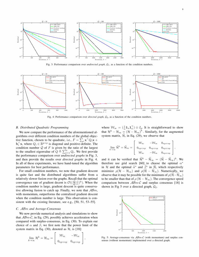
Fig. 3: Performance comparison over undirected graph, G1, as a function of the condition numbers.

0 200 400 600 800 100010-15

10-10

10-5

100

105

0 1000 2000 3000 4000 500010-15

10-10

10-5

100

105

0 2000 4000 6000 8000 1000010-15

10-10

10-5

100

105

Fig. 4: Performance comparison over directed graph, G2, as a function of the condition numbers.

B. Distributed Quadratic ProgrammingWe now compare the performance of the aforementioned al-

gorithms over different condition numbers of the global objec-tive function, chosen to be quadratic, i.e., F =

∑i x>Qix +

b>i x, where Qi ∈ Rp×p is diagonal and positive-definite. Thecondition number Q of F is given by the ratio of the largestto the smallest eigenvalue of Q ,

∑ni=1Qi. We first provide

the performance comparison over undirected graphs in Fig. 3,and then provide the results over directed graphs in Fig. 4.In all of these experiments, we have hand-tuned the algorithmparameters for best performance.

For small condition numbers, we note that gradient descentis quite fast and the distributed algorithms suffer from arelatively slower fusion over the graphs. Recall that the optimalconvergence rate of gradient decent is O((Q−1Q+1 )k). When thecondition number is large, gradient descent is quite conserva-tive allowing fusion to catch up. Finally, we note that ABm,with momentum, outperforms the centralized gradient descentwhen the condition number is large. This observation is con-sistent with the existing literature, see e.g., [50, 51, 53–55].

C. ABm and Average-ConsensusWe now provide numerical analysis and simulations to show

that ABm-C, in Eq. (29), possibly achieves acceleration whencompared with surplus-consensus, in Eq. (30). To explain ourchoice of α and β, we first note that the power limit of thesystem matrix in Eq. (30), denoted as H, is [18]:

limk→∞

Hk = H∞ =

W∞ −W∞0np×np 0np×np

,

where W∞ = ( 1n1n1

>n ) ⊗ Ip. It is straightforward to show

that Hk −H∞ = (H−H∞)k. Similarly, for the augmented

system matrix, H, in Eq. (29), we observe that

limk→∞

Hk = H∞ =

W∞ −W∞ 0np×np

0np×np 0np×np 0np×np

W∞ −W∞ 0np×np

,and it can be verified that Hk − H∞ = (H − H∞)k. Wetherefore use grid search [60] to choose the optimal α∗

in H and the optimal α∗ and β∗ in H, which respectivelyminimize ρ(H − H∞) and ρ(H − H∞). Numerically, weobserve that it may be possible for the minimum of ρ(H−H∞)to be smaller than that of ρ (H−H∞). The convergence speedcomparison between ABm-C and surplus consensus [18] isshown in Fig 5 over a directed graph, G2.

0 500 1000 1500 200010-15

10-10

10-5

100

105

Fig. 5: Average-consensus via ABm-C (with momentum) and surplus con-sensus (without momentum) implemented over a directed graph.

10

VII. CONCLUSIONS

In this paper, we provide a framework for distributed opti-mization that removes the need for doubly-stochastic weightsand thus is naturally applicable to both undirected and directedgraphs. Using a state transformation based on the non-1neigenvector, we show that the underlying algorithm, AB, basedon a simultaneous application of both RS and CS weights,lies at the heart of several algorithms studied earlier that relyon eigenvector estimation when using only CS (or only RS)weights. We then propose the distributed heavy-ball method,termed as ABm, that combines AB with a heavy-ball (type)momentum term. To the best of our knowledge, this paperis the first to use a momentum term based on the heavy-ball method in distributed optimization. We show that ABmsubsumes a novel average-consensus algorithm as a specialcase that unifies earlier attempts over directed graphs, withpotential acceleration due to the momentum term.

REFERENCES

[1] P. A. Forero, A. Cano, and G. B. Giannakis, “Consensus-based distributed support vector machines,” Journal of MachineLearning Research, vol. 11, no. May, pp. 1663–1707, 2010.

[2] S. Boyd, N. Parikh, E. Chu, B. Peleato, and J. Eckstein, “Dis-tributed optimization and statistical learning via the alternatingdirection method of multipliers,” Foundation and Trends inMaching Learning, vol. 3, no. 1, pp. 1–122, Jan. 2011.

[3] H. Raja and W. U. Bajwa, “Cloud k-svd: A collaborativedictionary learning algorithm for big, distributed data,” IEEETrans. on Signal Processing, vol. 64, no. 1, pp. 173–188, 2016.

[4] H.-T. Wai, Z. Yang, Z. Wang, and M. Hong, “Multi-agentreinforcement learning via double averaging primal-dual opti-mization,” arXiv preprint arXiv:1806.00877, 2018.

[5] A. Jadbabaie, J. Lin, and A. Morse, “Coordination of groups ofmobile autonomous agents using nearest neighbor rules,” IEEETrans. on Automatic Control, vol. 48, no. 6, pp. 988–1001, 2003.

[6] G. Mateos, J. A. Bazerque, and G. B. Giannakis, “Distributedsparse linear regression,” IEEE Trans. on Signal Processing,vol. 58, no. 10, pp. 5262–5276, Oct. 2010.

[7] J. A. Bazerque and G. B. Giannakis, “Distributed spectrumsensing for cognitive radio networks by exploiting sparsity,”IEEE Trans. on Signal Processing, vol. 58, no. 3, pp. 1847–1862, March 2010.

[8] M. Rabbat and R. Nowak, “Distributed optimization in sensornetworks,” in 3rd International Symposium on InformationProcessing in Sensor Networks, Berkeley, CA, Apr. 2004, pp.20–27.

[9] S. Safavi, U. A. Khan, S. Kar, and J. M. F. Moura, “Distributedlocalization: A linear theory,” Proceedings of the IEEE, 2018.

[10] J. Tsitsiklis, D. P. Bertsekas, and M. Athans, “Distributedasynchronous deterministic and stochastic gradient optimizationalgorithms,” IEEE Transactions on Automatic Control, vol. 31,no. 9, pp. 803–812, 1986.

[11] A. Nedic and A. Ozdaglar, “Distributed subgradient methods formulti-agent optimization,” IEEE Trans. on Automatic Control,vol. 54, no. 1, pp. 48–61, Jan. 2009.

[12] J. C. Duchi, A. Agarwal, and M. J. Wainwright, “Dual averagingfor distributed optimization: Convergence analysis and networkscaling,” IEEE Transactions on Automatic control, vol. 57, no.3, pp. 592–606, 2012.

[13] D. Kempe, A. Dobra, and J. Gehrke, “Gossip-based computa-tion of aggregate information,” in 44th Annual IEEE Symposiumon Foundations of Computer Science, Oct. 2003, pp. 482–491.

[14] K. I. Tsianos, S. Lawlor, and M. G. Rabbat, “Push-sum dis-tributed dual averaging for convex optimization,” in 51st IEEE

Annual Conference on Decision and Control, Maui, Hawaii,Dec. 2012, pp. 5453–5458.

[15] A. Nedic and A. Olshevsky, “Distributed optimization overtime-varying directed graphs,” IEEE Trans. on AutomaticControl, vol. 60, no. 3, pp. 601–615, Mar. 2015.

[16] C. Xi, Q. Wu, and U. A. Khan, “On the distributed optimizationover directed networks,” Neurocomputing, vol. 267, pp. 508–515, Dec. 2017.

[17] C. Xi and U. A. Khan, “Distributed subgradient projectionalgorithm over directed graphs,” IEEE Trans. on AutomaticControl, vol. 62, no. 8, pp. 3986–3992, Oct. 2016.

[18] K. Cai and H. Ishii, “Average consensus on general stronglyconnected digraphs,” Automatica, vol. 48, no. 11, pp. 2750 –2761, 2012.

[19] K. Yuan, Q. Ling, and W. Yin, “On the convergence ofdecentralized gradient descent,” SIAM Journal on Optimization,vol. 26, no. 3, pp. 1835–1854, Sep. 2016.

[20] A. S. Berahas, R. Bollapragada, N. S. Keskar, and E. Wei,“Balancing communication and computation in distributed op-timization,” arXiv preprint arXiv:1709.02999, 2017.

[21] E. Wei and A. Ozdaglar, “Distributed alternating directionmethod of multipliers,” in 51st IEEE Annual Conference onDecision and Control, Dec. 2012, pp. 5445–5450.

[22] J. F. C. Mota, J. M. F. Xavier, P. M. Q. Aguiar, and M. Puschel,“D-ADMM: A communication-efficient distributed algorithmfor separable optimization,” IEEE Trans. on Signal Processing,vol. 61, no. 10, pp. 2718–2723, May 2013.

[23] W. Shi, Q. Ling, K Yuan, G Wu, and W Yin, “On thelinear convergence of the admm in decentralized consensusoptimization,” IEEE Trans. on Signal Processing, vol. 62, no.7, pp. 1750–1761, April 2014.

[24] A. Mokhtari, W. Shi, Q. Ling, and A. Ribeiro, “A decentralizedsecond-order method with exact linear convergence rate for con-sensus optimization,” IEEE Trans. on Signal and InformationProcessing over Networks, vol. 2, no. 4, pp. 507–522, 2016.

[25] D. Jakovetic, J. Xavier, and J. M. F. Moura, “Fast distributedgradient methods,” IEEE Transactions on Automatic Control,vol. 59, no. 5, pp. 1131–1146, May 2014.

[26] W. Shi, Q. Ling, G. Wu, and W Yin, “Extra: An exact first-orderalgorithm for decentralized consensus optimization,” SIAMJournal on Optimization, vol. 25, no. 2, pp. 944–966, 2015.

[27] C. Xi and U. A. Khan, “DEXTRA: A fast algorithm foroptimization over directed graphs,” IEEE Trans. on AutomaticControl, vol. 62, no. 10, pp. 4980–4993, Oct. 2017.

[28] K. Yuan, B. Ying, X. Zhao, and A. H. Sayed, “Exact diffusionfor distributed optimization and learning—part i: Algorithmdevelopment,” arXiv preprint arXiv:1702.05122, 2017.

[29] K. Yuan, B. Ying, X. Zhao, and A. H. Sayed, “Exact diffusionfor distributed optimization and learning—part ii: Convergenceanalysis,” arXiv preprint arXiv:1702.05142, 2017.

[30] A. H. Sayed, “Diffusion adaptation over networks,” inAcademic Press Library in Signal Processing, vol. 3, pp. 323–453. Elsevier, 2014.

[31] J. Xu, S. Zhu, Y. C. Soh, and L. Xie, “Augmented distributedgradient methods for multi-agent optimization under uncoordi-nated constant stepsizes,” in IEEE 54th Annual Conference onDecision and Control, 2015, pp. 2055–2060.

[32] G. Qu and N. Li, “Harnessing smoothness to acceleratedistributed optimization,” IEEE Trans. on Control of NetworkSystems, Apr. 2017.

[33] C. Xi, R. Xin, and U. A. Khan, “ADD-OPT: Accelerateddistributed directed optimization,” IEEE Trans. on AutomaticControl, Aug. 2017, in press.

[34] A. Nedic, A. Olshevsky, and W. Shi, “Achieving geometric con-vergence for distributed optimization over time-varying graphs,”SIAM Journal of Optimization, Dec. 2017.

[35] C. Xi, V. S. Mai, R. Xin, E. Abed, and U. A. Khan, “Linearconvergence in optimization over directed graphs with row-stochastic matrices,” IEEE Trans. on Automatic Control, Jan.

11

2018, in press.[36] R. Xin, C. Xi, and U. A. Khan, “FROST – Fast row-

stochastic optimization with uncoordinated step-sizes,” Arxiv:https://arxiv.org/abs/1803.09169, Mar. 2018.

[37] R. Xin and U. A. Khan, “A linear algorithm for optimizationover directed graphs with geometric convergence,” IEEEControl Systems Letters, vol. 2, no. 3, pp. 325–330, Jul. 2018.

[38] G. Qu and N. Li, “Accelerated distributed Nesterov gradientdescent,” Arxiv: https://arxiv.org/abs/1705.07176, May 2017.

[39] D. Jakovetic, “A unification and generalization of exact dis-tributed first order methods,” IEEE Transactions on Signal andInformation Processing over Networks, 2018.

[40] H.-T. Wai, N. M. Freris, A. Nedic, and A. Scaglione, “Sucag:Stochastic unbiased curvature-aided gradient method for dis-tributed optimization,” arXiv preprint arXiv:1803.08198, 2018.

[41] M. Zhu and S. Martınez, “Discrete-time dynamic averageconsensus,” Automatica, vol. 46, no. 2, pp. 322–329, 2010.

[42] C. A. Desoer and M. Vidyasagar, Feedback systems: input-output properties, vol. 55, Siam, 1975.

[43] P. Di Lorenzo and G. Scutari, “Next: In-network nonconvex op-timization,” IEEE Trans. on Signal and Information Processingover Networks, vol. 2, no. 2, pp. 120–136, 2016.

[44] Y. Sun, G. Scutari, and D. Palomar, “Distributed nonconvexmultiagent optimization over time-varying networks,” in Sig-nals, Systems and Computers, 2016 50th Asilomar Conferenceon. IEEE, 2016, pp. 788–794.

[45] S. Pu, W. Shi, J. Xu, and A. Nedic, “A push-pull gradientmethod for distributed optimization in networks,” arXiv preprintarXiv:1803.07588, 2018.

[46] A. Priolo, A. Gasparri, E. Montijano, and C. Sagues, “A dis-tributed algorithm for average consensus on strongly connectedweighted digraphs,” Automatica, vol. 50, no. 3, pp. 946–951,2014.

[47] A. Nedic, A. Olshevsky, W. Shi, and C. A. Uribe, “Geomet-rically convergent distributed optimization with uncoordinatedstep-sizes,” in IEEE American Control Conference, May 2017.

[48] J. Xu, S. Zhu, Y. C. Soh, and L. Xie, “Convergence ofasynchronous distributed gradient methods over stochastic net-works,” IEEE Transactions on Automatic Control, vol. 63, no.2, pp. 434–448, 2018.

[49] Q. Lu, H. Li, and D. Xia, “Geometrical convergence rate fordistributed optimization with time-varying directed graphs anduncoordinated step-sizes,” Information Sciences, vol. 422, pp.516–530, 2018.

[50] B. Polyak, “Some methods of speeding up the convergenceof iteration methods,” USSR Computational Mathematics andMathematical Physics, vol. 4, no. 5, pp. 1–17, 1964.

[51] B. Polyak, Introduction to optimization, Optimization Software,1987.

[52] E. Ghadimi, H. R. Feyzmahdavian, and M. Johansson, “Globalconvergence of the heavy-ball method for convex optimization,”in Control Conference (ECC), 2015 European. IEEE, 2015, pp.310–315.

[53] M. Gurbuzbalaban, A. Ozdaglar, and P. A. Parrilo, “On the con-vergence rate of incremental aggregated gradient algorithms,”SIAM Journal on Optimization, vol. 27, no. 2, pp. 1035–1048,2017.

[54] L. Lessard, B. Recht, and A. Packard, “Analysis and designof optimization algorithms via integral quadratic constraints,”SIAM Journal on Optimization, vol. 26, no. 1, pp. 57–95, 2016.

[55] Y. Drori and M. Teboulle, “Performance of first-order methodsfor smooth convex minimization: a novel approach,” Mathe-matical Programming, vol. 145, no. 1-2, pp. 451–482, 2014.

[56] B. Polyak and P. Shcherbakov, “Lyapunov functions: Anoptimization theory perspective,” IFAC-PapersOnLine, vol. 50,no. 1, pp. 7456–7461, 2017.

[57] P. Tseng, “An incremental gradient (-projection) method withmomentum term and adaptive stepsize rule,” SIAM Journal onOptimization, vol. 8, no. 2, pp. 506–531, 1998.

[58] N. Loizou and P. Richtarik, “Linearly convergent stochasticheavy ball method for minimizing generalization error,” arXivpreprint arXiv:1710.10737, 2017.

[59] R. A. Horn and C. R. Johnson, Matrix Analysis, 2nd ed.,Cambridge University Press, New York, NY, 2013.

[60] Y. Nesterov, Introductory lectures on convex optimization: Abasic course, vol. 87, Springer Science & Business Media,2013.

[61] D. P. Bertsekas, Nonlinear programming, Athena scientificBelmont, 1999.

Ran Xin received his B.S. degree in Mathematicsand Applied Mathematics from Xiamen Univer-sity, China, in 2016, and M.S. degree in Electricaland Computer Engineering from Tufts Universityin 2018. Currently, he is a Ph.D. student in theElectrical and Computer Engineering departmentat Tufts University. His research interests includeoptimization theory and algorithms.

Usman A. Khan has been an Associate Professorof Electrical and Computer Engineering (ECE) atTufts University, Medford, MA, USA, since Septem-ber 2017, where he is the Director of Signal Pro-cessing and Robotic Networks laboratory. His re-search interests include statistical signal processing,network science, and distributed optimization overautonomous multi-agent systems. He has publishedextensively in these topics with more than 75 articlesin journals and conference proceedings and holdsmultiple patents. Recognition of his work includes

the prestigious National Science Foundation (NSF) Career award, severalNSF REU awards, an IEEE journal cover, three best student paper awardsin IEEE conferences, and several news articles. Dr. Khan joined Tufts as anAssistant Professor in 2011 and held a Visiting Professor position at KTH,Sweden, in Spring 2015. Prior to joining Tufts, he was a postdoc in theGRASP lab at the University of Pennsylvania. He received his B.S. degree in2002 from University of Engineering and Technology, Pakistan, M.S. degreein 2004 from University of Wisconsin-Madison, USA, and Ph.D. degree in2009 from Carnegie Mellon University, USA, all in ECE. Dr. Khan is an IEEEsenior member and has been an associate member of the Sensor Array andMultichannel Technical Committee with the IEEE Signal Processing Societysince 2010. He is an elected member of the IEEE Big Data special interestgroup and has served on the IEEE Young Professionals Committee and onIEEE Technical Activities Board. He was an editor of the IEEE Transactionson Smart Grid from 2014 to 2017, and is currently an associate editor ofthe IEEE Control System Letters. He has served on the Technical ProgramCommittees of several IEEE conferences and has organized and chairedseveral IEEE workshops and sessions.