Sponsored by the Bill & Melinda Gates Foundation

RAND American Educator Panels Technical Description

MICHAEL W. ROBBINS, DAVID MATTHEW GRANT

C O R P O R A T I O N

Print and Electronic Distribution Rights

This work is licensed under a Creative Commons Attribution 4.0 International License. All users of the publication are permitted to copy and redistribute the material in any medium or format and transform and build upon the material, including for any purpose (including commercial) without further permission or fees being required.

The RAND Corporation is a research organization that develops solutions to public policy challenges to help make communities throughout the world safer and more secure, healthier and more prosperous. RAND is nonprofit, nonpartisan, and committed to the public interest.

RAND’s publications do not necessarily reflect the opinions of its research clients and sponsors.

Support RANDMake a tax-deductible charitable contribution at

www.rand.org/giving/contribute

www.rand.org

For more information on this publication, visit www.rand.org/t/RR3104

Published (2020) by the RAND Corporation, Santa Monica, Calif.

R® is a registered trademark.

iii

Preface

Funding Funding for this project was provided by the Bill & Melinda Gates Foundation and by

income earned on client-funded research.

About This Report This report describes the methodology behind the RAND American Educator Panels, which

consist of the American School Leader Panel and the American Teacher Panel. It provides detailed information on the panels, the multiple phases and waves of recruitment used to create the panels, weighting, and variance estimation.

The project was undertaken within RAND Education and Labor, a division of the RAND Corporation that conducts research on early childhood through postsecondary education programs, workforce development, and programs and policies affecting workers, entrepreneurship, and financial literacy and decisionmaking.

Questions about this report should be directed to mrobbins@rand.org, and questions regarding RAND Education and Labor should be directed to educationandlabor@rand.org.

The findings and conclusions contained within are those of the authors and do not necessarily reflect positions or policies of the Bill & Melinda Gates Foundation. For more information and research on these and other related topics, please visit gatesfoundation.org.

iv

Contents

Preface ........................................................................................................................................... iiiFigures ............................................................................................................................................. vTables ............................................................................................................................................. viAbbreviations ............................................................................................................................... vii1. Introduction ................................................................................................................................. 12. Sampling ...................................................................................................................................... 2

Phase 1: The Westat School Sample ......................................................................................................... 3Phase 2: The Helmsley State-Level Teacher Oversample and Second Principal National Sample .......... 6Phase 3: The Gates MLI State-Level Oversample .................................................................................... 8

3. Weighting .................................................................................................................................. 18Inverse Probability Weighting ................................................................................................................ 19Design Weights ....................................................................................................................................... 21Covariates for the Nonresponse Models ................................................................................................. 22Calibration of Weights ............................................................................................................................ 25

4. Variance Estimation .................................................................................................................. 28Taylor Series Linearization ..................................................................................................................... 28Jackknife .................................................................................................................................................. 29

5. Conclusion ................................................................................................................................. 30References ..................................................................................................................................... 35

v

Figures

Figure 1. The History of ATP Recruitment ..................................................................................... 2Figure 2. The History of ASLP Recruitment ................................................................................... 3

vi

Tables

Table 1. The Teacher Recruitment Experiment: Strategies ........................................................... 10Table 2. The Teacher Recruitment Experiment: Results ............................................................... 11Table 3. 2016–2017 MLI Recruitment by State ............................................................................ 12Table 4. 2016–2017 MLI Recruitment by Batch ........................................................................... 13Table 5. 2018 ATP Recruitment .................................................................................................... 16Table 6. 2018 ASLP Recruitment ................................................................................................. 17Table 7. Results of Recruitment of Teachers and School Leaders by Timing of Recruitment,

2014–2018 ............................................................................................................................. 30Table 8. Results of Recruitment of Teachers and School Leaders by State, 2014–2018 .............. 31Table 9. Diagnostics Regarding the Number of Teachers per School Represented in the ATP ... 33

vii

Abbreviations

AEP American Educator Panels

ASLP American School Leader Panel ATP American Teacher Panel

CCD Common Core of Data IPW inverse probability weighting

MDR Market Data Retrieval MLI Measure to Learn and Improve

SASS Schools and Staffing Survey USPS U.S. Postal Service

1

1. Introduction

The RAND American Educator Panels (AEP) were created to provide the teacher and principal voice for evidence-based research on education policies and practices. The AEP are composed of the American Teacher Panel (ATP) and the American School Leader Panel (ASLP). These panels provide researchers with quick access to a large, high-quality sample of educators and allow those researchers to collect data from U.S. K–12 public school teachers and principals. The ATP is constituted of regular classroom teachers (excluding preschool teachers, resource teachers, athletic coaches, etc.) in K–12 public schools. Similarly, the ASLP focuses on principals (excluding assistant principals) leading K–12 public schools. Note that the panels include educators from various types of public schools, including charter and magnet schools, but not from private schools, special education schools, or continuation schools.

Research surveys are administered periodically to educators who have enrolled in one of the panels, which are mutually exclusive. A survey may be given to all members of a given panel or to a subset of the panel. Note that recruitment into the panels, which this report describes in detail, occurs separately from the administration of surveys to the panelists. There is no limit on the number of surveys that may be administered to a panelist once he or she has enrolled.

This report provides detailed information on the panels, the multiple phases and waves of recruitment used to create the panels, weighting, and variance estimation. Note that, although this report discusses weighting and variance estimation for surveys administered to the panels, we do not discuss sampling and response rates for such surveys. That is, all references here to sampling and response rates specifically relate to the recruitment of panelists, not to surveys administered to panelists.

2

2. Sampling

Teachers and school leaders have been recruited to join the AEP using probability-based sampling in several phases through 2018, as shown in Figures 1 and 2. Recruitment for both panels consists of three phases, with up to two waves per phase. The first phase for both panels (April 2014 through February 2015) incorporates two recruitment waves based on a school sample collected by Westat, and the third phase for both panels (October 2016 through May 2018) involves state-level oversampling in two waves sponsored by the Bill & Melinda Gates Foundation. For the ATP, the second phase consists of two waves of state-level oversampling sponsored by the Helmsley Foundation (July 2015 through April 2016); for the ASLP, the second phase consists of a single national sample sponsored by the RAND Corporation (February and March 2016).

Figure 1. The History of ATP Recruitment

Phase 1 Phase 2 Phase 3

NOTE: MLI = Measure to Learn and Improve.

April–May 2014

December 2014–

February 2015

July–August 2015

March–April 2016

WestatSchool

Sample: Wave 1

WestatSchool

Sample: Wave 2

State-level Oversample:

Helmsley Wave 1

State-level Oversample:

Helmsley Wave 2

State-level Oversample: Gates MLI

Wave 1

October 2016–March 2017

State-level Oversample: Gates MLI

Wave 2

February–May 2018

3

Figure 2. The History of ASLP Recruitment

Phase 1: The Westat School Sample

Wave 1 (Westat) School Sample (April–May 2014)

In early 2014, RAND contracted with Westat to design the ATP and ASLP. The initial recruitment plan for the panels, which was to be executed by Westat, proposed a multistage sampling approach. In the first stage, a sample of 2,300 public schools was drawn completely at random from the 2010–2011 Common Core of Data (CCD), which is produced by the National Center for Education Statistics. Westat contacted schools or districts as needed to obtain approval for research activities. Upon receipt of approval, contact information for a school’s principal and teachers was provided by the school. Westat contacted the principal at each sampled school and asked them to join the ASLP. In the second stage, two teachers at each school were randomly selected and asked to join the ATP. All 2,300 schools were sampled and then segmented into groups; the groups would represent a wave of sampling for principals and teachers (where waves are separated by timing of recruitment activities). The first wave would include approximately 800 schools.

Because a single sample of schools was used to recruit both principals and teachers, we had to decide how those schools would be sampled. For instance, schools could be invited to participate using simple random sampling (which would yield balanced representation for principals in the ASLP but lead to an overrepresentation of teachers at small schools in the ATP), or schools could be sampled with probability proportional to their teacher count (which would yield balanced representation for teachers in the ATP but would yield an underrepresentation of principals at small schools in the ASLP). Although the over- or underrepresentation of teachers and/or principals could be corrected in the weighting procedures, it would lead to a less statistically efficient design given the fixed size of the sample. As a compromise, an approach was carried out in which schools were sampled with probability proportional to the square root of their teacher count. Westat also oversampled novice teachers (those with three or fewer years

State-level Oversample: Gates MLI

Wave 2

April–May 2014

December 2014–February 2015

February–March 2016

Westat School

Sample: Wave 1

Westat School

Sample: Wave 2

Second Principal National Sample

State-level Oversample: Gates MLI

Wave 1

October 2016–March 2017

February–May 2018

4

of teaching experience) so that such teachers would constitute approximately 33 percent of the sample (we estimated that such teachers make up about 20 percent of the overall teacher population). Oversampling was done, in part, to hedge against the eventual aging of the panel. (Note that we do not, at any point, oversample novice principals.)

The sampling process described above required the procurement of district- and school-level approval for each sampled school. To hedge against the possibility that schools or districts would refuse, a list of replacement schools was compiled. Nonetheless, the requirement to gain approval at multiple levels (district, school, individual) provided several opportunities for refusal and/or nonresponse. During Wave 1 recruitment, which occurred in April and May 2014, 816 schools were sampled, of which district- and school-level approval was garnered for only 296 schools (36.2 percent, using American Association for Public Opinion Research Response Rate 1), including replacement schools.1 Teachers and principals at the 296 schools were sent letters inviting them to join the panels, and nonrespondents were recontacted by telephone at least four times. Two teachers were selected at random for each school, with novice teachers having a disproportionately higher probability of being selected. Of the 592 teachers contacted, 236 (39.9 percent) agreed to join the panel. Likewise, of the 299 principals contacted (some schools may have multiple principals), 145 (48.5 percent) agreed to join the panel. This yield is quite low when compared with the 1,632 teachers and 816 principals that would have enrolled under a 100-percent response rate. Thus, the effective recruitment rates are 14.5 percent for teachers and 17.8 percent for principals (where the effective response rate accounts for nonresponse at the district, school, and individual levels).

Wave 2 (Westat) School Sample (December 2014–February 2015)

In response to the low yield and lengthy procedures of the initial effort, we performed the next phase of recruitment of principals and teachers by fielding the remaining schools (from the original sample of 2,300 schools) in a single batch (referred to as Wave 2). To avoid undergoing the district- and school-level approval process and procuring contact lists from approving schools, we purchased contact information for all teachers and principals at the 2,300 schools that were part of the original sample but not used during Wave 1 from Market Data Retrieval (MDR), a market-research firm that specializes in the education sphere. There were 1,572 such schools (these included unused replacement schools that were sampled to supplement the original 2,300 schools). MDR stated that its databases had 95-percent coverage on all educators nationwide. Our research into this claim found that its databases were indeed more comprehensive than those provided by competing vendors.

We used RAND’s Survey Research Group to conduct Wave 2 recruitment; the principal and a variable number of teachers were contacted at each of the 1,572 schools. The number of

1 American Association for Public Opinion Research, Standard Definitions: Final Dispositions of Case Codes and Outcome Rates for Surveys, 9th ed., Oakbrook Terrace, Ill., revised 2016.

5

teachers contacted was larger at schools that had more teachers (on average, four teachers were contacted per school), with the goal of making the process mimic sampling with probability proportional to size.2 For this Wave 2 recruitment, 1,572 principals and 6,590 teachers were mailed a recruitment package that included a brochure and a letter inviting them to enroll in the ASLP and ATP, respectively. Principals and teachers were also promised a $10 electronic gift card if they enrolled.3 Two email follow-ups were sent to nonresponders. This process yielded 200 principals (13.0-percent response rate) and 722 enrolled teachers (11.0-percent response rate); note that these rates were slightly lower than the effective recruitment rates noted above for the Westat recruitment for Wave 1. Also note that oversampling of novice teachers was not implemented at this stage because we were unable to obtain reliable experience data on teachers from MDR.

Because of low recruitment rates during the early fielding of this sampling effort, an experiment was implemented to more directly compare methods of recruitment and determine the most cost-effective method moving forward. Details of the experiment are described comprehensively in Robbins et al., 2018; relevant information is paraphrased below.4

Recruitment Experiment

Because of the low response to recruitment efforts in the early part of Wave 2, alternative methods of recruitment were considered. We performed an experiment in which a variety of recruitment methods were attempted with the remaining teachers who had not been contacted in the first part of Wave 2. These teachers were sampled at random using a probability proportional to size scheme similar to the one used to initially sample in Wave 2. Because we had exhausted our list of contact information for principals at sampled schools, rigorous refusal conversion on nonresponding principals was attempted.

The teacher experiment contained four separate arms. Each of the following arms contained 250 teachers:

1. Teachers were sent a $10 Target gift card as a preincentive (i.e., all recipients were provided the gift card with the initial recruitment package, regardless of participation).

2. Teachers were sent a $20 Target gift card as a preincentive. 3. Teachers were sent a $20 electronic gift card as a preincentive. 4. Teachers were contacted by telephone and asked to join the panels.

2 This was effectively a probability proportional to size sampling scheme. That is, n = cN, in which n is the number of teachers sampled from a school with N total teachers, and c is a constant for all schools and was selected so that, on average, four teachers per school were sampled. 3 The electronic gift card option allowed the recipient to choose a provider among multiple vendors. 4 Michael W. Robbins, Geoffrey Grimm, Brian Stecher, and V. Darleen Opfer, “A Comparison of Strategies for Recruiting Teachers into Survey Panels,” SAGE Open, August 22, 2018.

6

All mailed packets were sent to Arms 1, 2, and 4 using FedEx. There was only email contact (no mailing) for Arm 3. Two email follow-ups with nonresponders were used for all groups. Further details are provided in Robbins et al., 2018.

The third and fourth arms had low success rates—Arm 3 yielded a 1.5-percent response rate, and Arm 4 yielded a 15.6-percent response rate—and were excluded from further consideration. The first arm had a response rate of 21.2 percent, while the second arm was the most successful, with a response rate of 22.8 percent. However, we preferred the strategy used in the first arm; it was the most cost-effective and was not significantly less successful than the second arm. Contact information was incorrect for a fairly substantial number of contacted teachers—22 percent by our estimates (note that contact information was largely correct for principals). The accuracy of contact information was assessed using the telephone group, in which a school’s central office, which was contacted by telephone, revealed whether the teacher was at the school. (We saw no instances in which telephone information was incorrect but email contact information was correct.) As such, the effective recruitment rate of the first strategy was 27.2 percent. In total, 159 teachers were recruited across the four arms of the experiment.

To account for the possibility that our preferred strategy of a $10 preincentive might be useful as a means of refusal conversion, we randomly sampled 250 nonresponding teachers from the first phase of Westat Wave 2 recruitment. These teachers were again recruited using the preferred strategy; however, this process only yielded 28 new enrollees (for a success rate of 11.2 percent) and was not pursued further. Finally, using remaining funds, we sampled 2,500 additional teachers from the lists we purchased for the 1,572 schools (sampling was again performed in a manner proportional to school size). These teachers were recruited using the preferred strategy of a $10 preincentive; an additional 492 teachers were enrolled (for a success rate of 19.7 percent).

For principals, in lieu of sampling new schools, which would yield new principals to recruit, we followed up with nonrespondents from the first stages of Wave 2 via telephone and encouraged them to enroll in the ASLP. This yielded an additional 179 panelists (bringing our rate of successful recruitment of principals to 24.8 percent of the 1,572 contacted at this stage). We also selected 250 of the principals who had not enrolled by this point and sent them $10 Target gift cards as a preincentive, but this only yielded 23 additional panelists; this effort was not cost-effective and was not considered further.

Phase 2: The Helmsley State-Level Teacher Oversample and Second Principal National Sample

Wave 1 Helmsley State-Level Oversample (July–August 2015)

Because of the needs of a specific project (funded by the Helmsley Charitable Trust), additional recruitment was conducted in four target states (California, Louisiana, New Mexico,

7

and New York) in July 2015. Using a sample frame purchased from MDR, we targeted 400 enrolled panelists in each of these states (including existing panelists); such a sample size would yield a maximum margin of error of 7–8 percent for state-level analyses from surveys administered to the ATP (note that this margin of error accounts for nonresponse among panelists). Furthermore, because the Helmsley project was largely concerned with analyses involving teachers of core subjects, we segmented the teacher population in each state into six mutually exclusive groups as follows based on information provided by MDR:

1. elementary school teachers listed as teaching math or English language arts or not listed as teaching any specific subject(s)

2. elementary school teachers not included above 3. non–elementary school math or English language arts teachers 4. non–elementary school science or social studies teachers 5. non–elementary school teachers of subjects not included above 6. non–elementary school teachers with a missing subject.

For this stage of recruitment, we oversampled from segments 1, 3, and 4 and undersampled from the other segments.

Sampling for this recruitment effort was performed using single-stage sampling—that is, we did not first select schools and then select teachers from those schools. We asked the vendor to stratify the teachers in its database according to the segments described above and then to randomly select a prespecified number of teachers from each segment. Using this process, 6,200 teachers were sampled, which was deemed necessary to reach our targets while accounting for a presumed 20-percent response rate and the number of existing panelists in each state. The sampled teachers were sent a FedEx packet that contained a brochure, a recruitment letter, and a $10 Target gift card (our preferred method identified from the recruitment experiment described above). We sent follow-up emails to nonresponders where email addresses were provided by MDR. This process yielded 1,248 new panelists, for a success rate of 20.1 percent. As part of a supplemental recruitment effort, an additional 2,199 teachers were contacted using email only (no recruitment package was sent by FedEx) and a promised incentive of a $10 electronic gift card was offered because of financial constraints; only 82 enrolled, for a response rate of 3.7 percent.

Wave 2 Helmsley State-Level Oversample (March–April 2016)

Following completion of the recruitment described above (Helmsley round 1), the Helmsley foundation decided to fund supplemental ATP recruitment of teachers in each of the four target states. The goal at this stage was to procure a sample of 550 panelists (in the ATP overall) in each state to obtain a maximum margin of error of 6 percent for state-level analyses of surveys administered to the panel. To achieve this, 2,300 teachers were contacted using a sampling frame purchased from MDR, and we followed the same processes used in the earlier Helmsley

8

recruitment. This effort led to the successful recruitment of 576 additional panelists, for a response rate of 25.0 percent.

The total numbers of ATP panelists enrolled across all recruitment efforts as of April 2016 are:

• California: 524 • Louisiana: 506 • New Mexico: 498 • New York: 553 • other: 1,462.

The Second Principal National Sample (February–March 2016)

We provided funding to facilitate the growth of the educator panels and recruited additional principals in February and March 2016. We randomly selected 3,000 schools from across the nation (excluding schools with previously contacted principals) using the CCD and contacted the principal at each school. We again used our preferred method from the recruitment experiment conducted for the Helmsley projects (i.e., we sent each principal a FedEx packet that contained a brochure, recruitment letter, and a $10 Target gift card). Of 3,001 contacted principals, 800 (26.7 percent) agreed to join the ASLP. As of March 2016, a total of 1,340 panelists had enrolled in the ASLP.

Phase 3: The Gates MLI State-Level Oversample

Gates MLI Recruitment of Teachers and Principals (October 2016–March 2017)

From October 2016 to March 2017, a larger recruitment effort was implemented in which a total of 103,729 educators were contacted and asked to join the panels (63,299 teachers and 40,430 principals). We used single-stage sampling here. That is, teachers and principals were selected at random from within an entire state. The principal and teacher samples were drawn independently. This recruitment was performed to facilitate state-level analyses for both teachers and principals from a series of MLI surveys sponsored by the Bill & Melinda Gates Foundation within targeted states. The target states are Alabama, Arkansas, California, Colorado, Delaware, Florida, Georgia, Illinois, Kentucky, Louisiana, Maryland, Massachusetts, Mississippi, New Mexico, New York, North Carolina, Oklahoma, South Carolina, Tennessee, Texas, Virginia, and West Virginia. New York City was analyzed separately from the rest of New York, so it was oversampled as well. A principal sample was not fielded in Colorado.

Sampling

Power analyses indicated that 800 teacher panelists were needed in each target state to facilitate the desired analyses. Furthermore, we wanted 1,100 principal panelists from these states because our experience fielding teacher and principal surveys revealed that principals

9

respond to surveys at lower rates than teachers (i.e., we anticipated that 42 percent of the ASLP would respond to the MLI survey, whereas 65 percent of the ATP would respond).

We anticipated that 25 percent of both teachers and principals contacted would enroll in the respective panel based on prior recruitment experience. Therefore, we contacted a maximum of 3,200 teachers in each state (in most cases, we made fewer contacts to account for existing panelists). Similarly, we needed to contact 4,400 principals in each state to reach our desired number of panelists. However, only California, New York, and Texas had that many principals available. Therefore, census sampling (i.e., inviting everyone) was conducted for principals in each target state other than California and Texas (creating a sample for New York City mandated that we perform census sampling in New York State as a whole as well).

To help reduce the effect of the aging of the panel over time, we stratified the teacher sample on the basis of experience level in states where experience information was available. These states are Arkansas, Florida, Georgia, Louisiana, Mississippi, and Tennessee. The experience-based strata were defined as follows:

1. three years of experience or less 2. more than three years of experience 3. experience missing.

In the remaining states, we stratified based on age, in which age-based strata are defined as:

1. less than 30 years of age 2. at least 30 years of age 3. age missing.

Sampling was performed so that inexperienced and younger teachers were moderately oversampled.

Recruitment Procedures

The contact information (including names, school addresses, and email addresses) of principals was obtained from publicly available administrative data for Alabama, Arkansas, California, Florida, Georgia, Massachusetts, Mississippi, New Mexico, New York, North Carolina, Oklahoma, and South Carolina. Similarly, we obtained contact information for North Carolina teachers directly from the state department of education. In all other cases, we purchased contact information from MDR. However, the vendor could not provide email addresses for teachers in Delaware. In states in which we performed oversampling, there were instances in which we knew that a school existed (as indicated by the CCD), but we were not able to find contact information for the principal via the aforementioned approaches. In these cases, we mailed recruitment materials to the school addressed simply to “Principal”; we were unable to send follow-up reminders via email in these cases. Single-stage sampling was again used and the principal and teacher samples were drawn independently.

Using the single-stage sampling approach, recruitment packages were mailed in 16 batches (of approximately 6,500 educators per batch) weekly, beginning on October 20, 2016 (no

10

mailings were sent during the winter break). The same recruitment methods used during Phase 2 as described above (i.e., FedEx mailing with $10 Target gift card, six follow-up emails to nonresponders) were used for most educators contacted during the 2016–2017 MLI recruitment. This procedure was not used for some individuals included in an experiment outlined later in this report, as well as in cases in which we did not have sufficient contact information and could not send follow-up emails. In the latter case, two follow-up letters were sent via postal mail. The determination of which educators would be part of the 16 batches was random, with the exception of the 16th batch, which included all educators who could not be contacted via email (i.e., teachers in Delaware and principals at schools where nothing was known about the principal). Endorsement letters from national educator unions (including the National Education Association and American Federation of Teachers for teachers, and National Association of Elementary School Principals, National Association of Secondary School Principals, and the School Superintendents Association for principals) were included in the packages for all educators, and endorsement letters from the educator’s state department of education were included in the package for educators in North Carolina and Oklahoma.

MLI Teacher Recruitment Experiment

Because of the magnitude of the MLI recruitment effort, we wanted to be certain that the optimal recruitment approach was used. Because the prior experiment was limited in scope, we designed a new experiment in which many recruitment methods were used. This experiment was performed during the first batch of recruitment so that if one method was found to outperform our preferred approach, we could use it for later waves. The recruitment methods considered are described in Table 1.

Table 1. The Teacher Recruitment Experiment: Strategies

Incentive Mode of Contact Group Brief Description Preincentive Promised

1 Standard $10 Target gift card FedEx 2 USPS standard $10 Target gift card USPS 3 Cash preincentive $10 cash USPS

4 $40 Target gift card promised

$40 Target gift card FedEx

5 $60 Target gift card promised

$60 Target gift card FedEx

6 Check promised $40 check FedEx

7 Electronic gift card promised

$40 (electronic gift card) FedEx

8 Combination $2 cash $40 Target gift card USPS 9 ATP reporta $10 Target gift card FedEx 10 Email-lessb $10 Target gift card FedEx NOTE: USPS = U.S. Postal Service a A copy of a research report on state standards is included in the recruitment package. b We do not follow-up with nonrespondents via email. They are sent two reminders via the USPS. Other respondents are sent up to six email follow-up reminders.

11

The standard procedure (experimental group 1) was our preferred approach at the onset of the experiment based on our prior experiment and therefore was administered to the largest number of teachers. The groups differed based on the type of incentive used as well as the mode of contact. For instance, we used preincentives (which are sent to all contacted educators), promised incentives (which are sent only to those who enroll), and a combination of both. We also varied the incentive payment method (i.e., cash, check, gift cards) and the payment amounts. Also considered and varied was the mode of delivery, using FedEx and postal mail (USPS). The results from the experiment are shown in Table 2.

Table 2. The Teacher Recruitment Experiment: Results

Response Rate Cost per Recruited Panelist Strategy n Estimate Standard Error p-valuea Estimate Standard Error p-valuea 1 Standard 1,213 27.6% 1.3% — $66.55 $3.09 —

2 USPS standard 250 18.8% 2.8% 0.004 $80.85 $10.63 0.196

3 Cash preincentive 250 23.2% 2.7% 0.151 $65.52 $7.54 0.899

4 $40 Target gift card promised 250 16.8% 2.4% 0.000 $91.97 $7.02 0.001

5 $60 Target gift card promised 250 19.6% 2.5% 0.009 $104.85 $5.48 0.000

6 Check promised 250 20.0% 2.5% 0.013 $83.99 $5.30 0.004

7 Electronic gift card promised 250 22.0% 2.6% 0.068 $78.09 $4.54 0.036

8 Combination 250 19.2% 2.5% 0.006 $79.59 $4.86 0.024

9 ATP report 250 26.8% 2.8% 0.792 $79.78 $8.34 0.137

10 Email-less 250 24.0% 2.7% 0.241 $101.88 $11.47 0.003 NOTE: Standard errors and p-values for raw recruitment rates (noncumulative) are calculated using the normal approximation to the binomial. Cost per recruit is calculated using the (multivariate) delta method. For example, if the raw recruitment rate for a strategy is �̂�𝑝 and if the strategy costs $𝐴𝐴 per educator contacted (with no costs incurred on a per-recruit basis), the estimated cost per recruit is given by 𝐴𝐴/�̂�𝑝 and the standard error of the estimated cost is given by 𝐴𝐴&(1 − �̂�𝑝)/(𝑛𝑛�̂�𝑝!). a p-values provide comparisons to strategy 1.

The experiment yielded several compelling findings. First, preincentives clearly outperform

promised incentives, which has been well established in the literature and was evident from our earlier experiment. Our results show that a $10 preincentive yields a rate of response that is 65 percent higher than the rate resulting from a $40 promised incentive. As such, the preincentive is markedly more cost-effective, even though overall response rates are seemingly low (meaning the preincentive is sent to a large portion of recruits who do not enroll). In addition, the use of FedEx is dramatically more effective than postal mail (e.g., group 1 has a response rate that is 47 percent higher than group 2). Furthermore, cash and check appear to perform better than gift cards, but not dramatically so. The email-less strategy yielded a slightly lower response rate than the standard approach, but it was much less cost-effective.

12

To summarize the experiment’s findings, we see that a preincentive outperforms a promised incentive, cash is the preferred format of incentive (followed by check), and FedEx is the preferred mode of mailing. Therefore, because cash cannot be sent via FedEx, the only way to improve upon our standard approach (without increasing the amount of the preincentive) would be to use a check in place of a Target gift card as a preincentive (note that this specific condition was not tested). However, the estimated improvement was not deemed substantial enough to warrant the requisite loss in efficiency (obtaining personalized checks is more time consuming and costly than obtaining a mass of gift cards). Therefore, we continued using the standard strategy throughout the remainder of the 2016–2017 MLI recruitment.

Recruitment Results

The overall results of the 2016–2017 MLI recruitment expansion are shown by state in Table 3 for teachers and principals. Recruitment was more successful for teachers than principals (30.9 percent versus 24.7 percent). Teacher recruitment exceeded the goal of 25 percent, and principal recruitment nearly met this goal. Note that principals probably would have cleared this threshold were it not for insufficient contact information (e.g., no email addresses) for 4,835 principals. Among those principals, the enrollment rate was 21.7 percent. There was notable variation in response rates across states. North Carolina observed the highest success rate (42.1 percent for teachers and 35.1 percent for principals), likely because of the use of state-level endorsement letters and because teacher contact information was provided by the state. We also observed high response rates in Oklahoma, which was the other state where endorsement letters were used. The lowest enrollment rates for teachers were observed in New York. Low recruitment rates also were observed for teachers in Delaware, which is likely a consequence of our inability to obtain email addresses for those teachers.

Table 3. 2016–2017 MLI Recruitment by State

Teachers Principals

State Number

Contacted Number Enrolled Rate

Number Contacted

Number Enrolled Rate

Alabama 3,108 907 29.2% 1,287 277 21.5% Arkansas 3,100 1,054 34.0% 979 287 29.3% California 1,459 380 26.0% 3,873 947 24.5% Colorado 3,090 937 30.3% 0 0 — Delaware 3,008 732 24.3% 196 44 22.4% Florida 2,947 919 31.2% 3,415 790 23.1% Georgia 2,762 841 30.4% 2,152 510 23.7% Illinois 2,931 1,023 34.9% 3,718 1,036 27.9% Kentucky 3,100 968 31.2% 1,186 314 26.5% Louisiana 1,244 325 26.1% 1,277 245 19.2% Maryland 3,121 955 30.6% 1,268 234 18.5%

13

Teachers Principals

State Number

Contacted Number Enrolled Rate

Number Contacted

Number Enrolled Rate

Massachusetts 3,052 794 26.0% 1,703 374 22.0% Mississippi 3,143 948 30.2% 896 257 28.7% New Mexico 1,322 389 29.4% 884 210 23.8% New York 5,204 1,243 23.9% 4,400 876 19.9% North Carolina 2,813 1,183 42.1% 2,413 846 35.1% Oklahoma 3,047 1,110 36.4% 1,604 510 31.8% South Carolina 3,121 1,072 34.3% 1,140 304 26.7% Tennessee 2,996 1,075 35.9% 1,763 521 29.6% Texas 2,601 702 27.0% 3,999 801 20.0% Virginia 2,976 959 32.2% 1,618 398 24.6% West Virginia 3,151 1,071 34.0% 659 194 29.4% Total 63,296 19,587 30.9% 40,430 9,975 24.7%

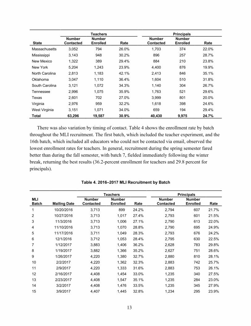
There was also variation by timing of contact. Table 4 shows the enrollment rate by batch

throughout the MLI recruitment. The first batch, which included the teacher experiment, and the 16th batch, which included all educators who could not be contacted via email, observed the lowest enrollment rates for teachers. In general, recruitment during the spring semester fared better than during the fall semester, with batch 7, fielded immediately following the winter break, returning the best results (36.2-percent enrollment for teachers and 29.8 percent for principals).

Table 4. 2016–2017 MLI Recruitment by Batch

MLI Batch Mailing Date

Teachers Principals Number

Contacted Number Enrolled Rate

Number Contacted

Number Enrolled Rate

1 10/20/2016 3,713 899 24.2% 2,794 607 21.7% 2 10/27/2016 3,713 1,017 27.4% 2,793 601 21.5% 3 11/3/2016 3,713 1,006 27.1% 2,790 613 22.0% 4 11/10/2016 3,713 1,070 28.8% 2,790 695 24.9% 5 11/17/2016 3,711 1,049 28.3% 2,793 676 24.2% 6 12/1/2016 3,712 1,053 28.4% 2,795 630 22.5% 7 1/12/2017 3,883 1,406 36.2% 2,628 783 29.8% 8 1/19/2017 3,882 1,366 35.2% 2,627 751 28.6% 9 1/26/2017 4,220 1,380 32.7% 2,880 810 28.1% 10 2/2/2017 4,220 1,362 32.3% 2,883 742 25.7% 11 2/9/2017 4,220 1,333 31.6% 2,883 753 26.1% 12 2/16/2017 4,408 1,454 33.0% 1,235 340 27.5% 13 2/23/2017 4,408 1,547 35.1% 1,235 284 23.0% 14 3/2/2017 4,408 1,476 33.5% 1,235 345 27.9% 15 3/9/2017 4,407 1,445 32.8% 1,234 295 23.9%

14

MLI Batch Mailing Date

Teachers Principals Number

Contacted Number Enrolled Rate

Number Contacted

Number Enrolled Rate

16 3/16/2017 2,968 724 24.4% 4,835 1,050 21.7% Total 63,299 19,587 30.9% 40,430 9,975 24.7%

Wave 2 Gates MLI Recruitment (February–May 2018)

Additional MLI recruitment was conducted in advance of the 2018 MLI survey (administered in May 2018). The 2018 MLI recruitment used the same general recruitment approach as the previous MLI recruitment, starting with a FedEx recruitment package that included a $10 Target gift card, an invitation letter, and endorsement letters.

The 2018 MLI recruitment had the following four overall goals:

1. Add teacher oversamples in three additional states: Nebraska, Rhode Island, and Wisconsin (funding for adding these three states was provided by the Bill & Melinda Gates Foundation and the Charles and Lynn Schusterman Family Foundation).

2. Achieve modest recruitment of teachers and school leaders in the 22 oversampled states to offset attrition.

3. Increase the national sample of teachers and school leaders to better balance the national sample with the state oversample recruitment focus of the 2016–2017 recruitment; this was meant to improve the overall design-effect caused by the oversampling of 22 states in the 2016–2017 recruitment.

4. Oversample novice teachers.

The recruitment targets for 2018 were different for the ATP and the ASLP: The fourth goal applied only to the ATP.

Oversampling of Novice Teachers

It is concerning to the AEP research team that inexperienced teachers may be underrepresented in the ATP (with more-dramatic underrepresentation of first-year teachers). There are two primary causes: First, the panel ages naturally, such that novice teachers become experienced, and second, novice teachers leave the profession at higher rates than more-experienced teachers.5 Furthermore, the databases used for sampling frames (e.g., MDR) are inherently out of date to some degree and therefore represent fewer newer teachers. Therefore, in the 2018 recruitment effort, we attempted to correct underrepresentation of newer teachers by oversampling novice teachers. However, experience information is missing from or inaccurate for much of the MDR database (MDR has no information on the experience level of approximately 60 percent of the teachers).

5 Matthew Ronfeldt, Susanna Loeb, and James Wyckoff, “How Teacher Turnover Harms Student Achievement,” American Educational Research Journal, Vol. 50, No. 1, 2013; Linda Darling-Hammond and Gary Sykes, “Wanted: A National Teacher Supply Policy for Education: The Right Way to Meet the ‘Highly Qualified Teacher’ Challenge,” Education Policy Analysis Archives, Vol. 11, No. 33, 2003.

15

For each oversampled state, we requested contact information for four times as many teachers as we would attempt to recruit (assuming a 25-percent recruitment rate). We sorted these teachers using three characteristics, which should be indicative to some degree of level of experience. These are

1. teaching experience (in years): missing for 57 percent of teachers and sometimes inaccurate. A novice teacher is one with three or fewer years of experience.

2. teacher age (in years): missing for 30 percent of teachers and sometimes inaccurate. A young teacher is one that is 30 years old or younger.

3. time in the MDR database (in years): missing for 0 percent of teachers. A new entry teacher is one who has been in the MDR database for two or fewer years.

From these three variables, we created a composite variable that takes on one of the following categories (the categories are mutually exclusive):

1. the teacher is a novice (with experience nonmissing): 9 percent of teachers 2. the teacher is not a novice (with experience nonmissing): 73 percent of teachers 3. the teacher is young and is a new entry (with experience missing and age nonmissing): 1

percent of teachers 4. the teacher is not young and is a new entry (with experience missing and age

nonmissing): 2 percent of teachers 5. the teacher is a new entry (with both experience and age missing): 3 percent of teachers 6. the teacher is not a new entry (with both experience and age missing): 13 percent of

teachers. We then randomly sampled teachers to recruit from the data file provided by MDR at

disparate rates. Teachers in the first and third categories were considered to have a high probability of being an inexperienced teacher. Therefore, these teachers were sampled at high rates. Teachers in the fourth and fifth categories were considered to have a moderate probability of being an inexperienced teacher and were therefore sampled at moderate rates. Teachers in the second and sixth category were considered to have a low probability of being an inexperienced teacher; such teachers were sampled at a low rate. Note that all teachers included in the 2018 MDR data file had a nonzero probability of being recruited. The specific sampling probabilities used varied by state depending on the availability of experience and age data. However, the composition of those sampled as part of the refresh within MLI states was, by the six categories: (1) 37 percent, (2) 12 percent, (3) 8 percent, (4) 10 percent, (5) 27 percent, and (6) 6 percent.

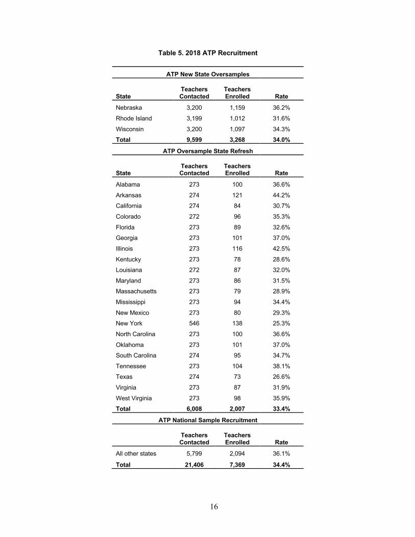
Recruitment Results

Tables 5 and 6 show the number of teachers and principals contacted as part of the 2018 recruitment effort, the number enrolled, and the success rate of enrolling teachers and principals invited to join the panels.

16

Table 5. 2018 ATP Recruitment

ATP New State Oversamples

State Teachers Contacted

Teachers Enrolled Rate

Nebraska 3,200 1,159 36.2%

Rhode Island 3,199 1,012 31.6%

Wisconsin 3,200 1,097 34.3%

Total 9,599 3,268 34.0%

ATP Oversample State Refresh

State Teachers Contacted

Teachers Enrolled Rate

Alabama 273 100 36.6%

Arkansas 274 121 44.2%

California 274 84 30.7%

Colorado 272 96 35.3%

Florida 273 89 32.6%

Georgia 273 101 37.0%

Illinois 273 116 42.5%

Kentucky 273 78 28.6%

Louisiana 272 87 32.0%

Maryland 273 86 31.5%

Massachusetts 273 79 28.9%

Mississippi 273 94 34.4%

New Mexico 273 80 29.3%

New York 546 138 25.3%

North Carolina 273 100 36.6%

Oklahoma 273 101 37.0%

South Carolina 274 95 34.7%

Tennessee 273 104 38.1%

Texas 274 73 26.6%

Virginia 273 87 31.9%

West Virginia 273 98 35.9%

Total 6,008 2,007 33.4%

ATP National Sample Recruitment

Teachers Contacted

Teachers Enrolled Rate

All other states 5,799 2,094 36.1%

Total 21,406 7,369 34.4%

17

Table 6. 2018 ASLP Recruitment

ASLP Oversample State Refresh

State Principals Contacted

Principals Enrolled Rate

Alabama 174 35 20.1%

Arkansas 207 56 27.1%

California 110 26 23.6%

Delaware 12 2 16.7%

Florida 433 84 19.4%

Georgia 211 44 20.9%

Illinois 325 79 24.3%

Kentucky 140 36 25.7%

Louisiana 137 35 25.5%

Maryland 130 29 22.3%

Massachusetts 263 60 22.8%

Mississippi 67 17 25.4%

New Mexico 111 22 19.8%

New York 443 74 16.7%

North Carolina 375 115 30.7%

Oklahoma 290 76 26.2%

South Carolina 193 51 26.4%

Tennessee 198 52 26.3%

Texas 51 11 21.6%

Virginia 132 31 23.5%

West Virginia 35 3 8.6%

Total 4,037 938 23.2%

ASLP National Sample Recruitment

Principals Contacted

Principals Enrolled Rate

All other states 4,563 1,166 25.6%

18

3. Weighting

In this section, we describe the steps we took to create weights for surveys conducted with the panels and for the different recruitment waves as the panels were created. Weighting is necessary because unadjusted ATP/ASLP survey data (once a survey is administered to one of the panels) may not represent the respective educator populations because of oversampling of certain types of educators and response rates (at both the recruitment stage and survey administration stage) that may differ across various educator characteristics. Furthermore, if there are biases inherent in the sample frame that was used, those will be transferred to the survey data. Therefore, respondents to surveys administered to the panels are assigned weights to ensure that survey responses appropriately represent the educator population of interest, such as the national set of K–12 public school teachers. Note that because survey administered to the panels is assumed to contain a different set of respondents (e.g., some panelists refuse to take a given survey, and the refusing panelists vary by survey), a new set of weights is calculated for each survey.

Before 2017, weights for the ATP and ASLP were calculated using inverse probability weighting (IPW)—that is, a survey respondent’s weight was calculated as equal to the inverse of the respondent’s probability of being among the pool of respondents to the survey. A complicating factor for IPW is that the panels were built through multiple recruitment efforts across several separate samples. The separate samples for the ATP are

1. the Wave 1 and Wave 2 Westat school samples (combined into a single sample for weighting)

2. the Helmsley Wave 1 and Wave 2 state-level oversamples (combined into a single sample for weighting)

3. the Gates 2016–2017 MLI state-level oversample 4. the Gates 2018 MLI state-level refresh and national sample. For the ASLP, the samples are

1. the Wave 1 and Wave 2 Westat school samples (combined into a single sample for weighting)

2. the second principal national sample 3. the Gates 2016–2017 MLI state-level oversample 4. the Gates 2018 MLI state-level refresh and national sample.

To determine IPW weights, each sample is weighted individually to be representative at the state level (for oversampled states—nonoversampled states are combined). The separately weighted samples are then merged in an appropriate manner as outlined below. For surveys administered in 2017 and after, the IPW weights were calibrated to ensure that the weighted survey data match known benchmarks; this is done to account for any discrepancies between the

19

sampling frame and the population. For surveys administered in 2017 and after, replication weights are calculated that facilitate estimation of uncertainty (e.g., standard errors, variances, margins of error, coefficients of variation). IPW and the steps for merging samples are described in the following subsection. IPW mandates the inclusion of design weights (which are discussed in the subsection following the discussion on IPW) as well as estimates of nonresponse probabilities (models for such estimates are described following the subsection on design weights).

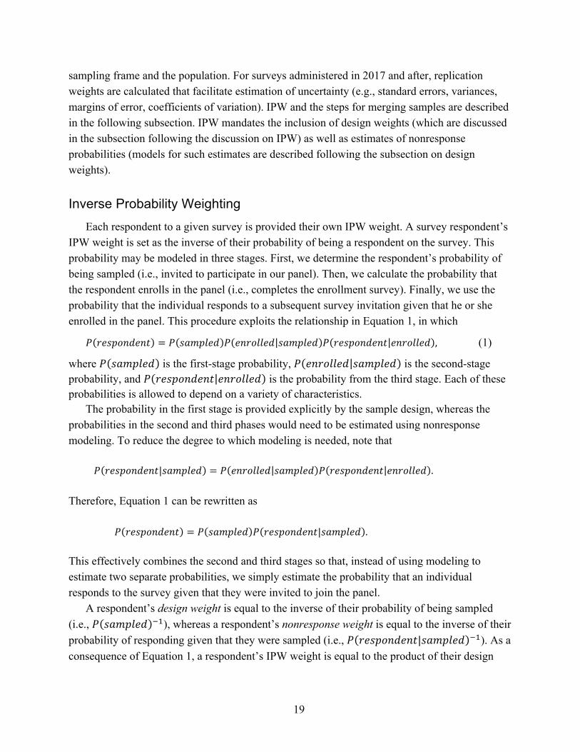
Inverse Probability Weighting Each respondent to a given survey is provided their own IPW weight. A survey respondent’s

IPW weight is set as the inverse of their probability of being a respondent on the survey. This probability may be modeled in three stages. First, we determine the respondent’s probability of being sampled (i.e., invited to participate in our panel). Then, we calculate the probability that the respondent enrolls in the panel (i.e., completes the enrollment survey). Finally, we use the probability that the individual responds to a subsequent survey invitation given that he or she enrolled in the panel. This procedure exploits the relationship in Equation 1, in which

𝑃𝑃(𝑟𝑟𝑟𝑟𝑟𝑟𝑟𝑟𝑟𝑟𝑟𝑟𝑟𝑟𝑟𝑟𝑟𝑟𝑟𝑟) = 𝑃𝑃(𝑟𝑟𝑠𝑠𝑠𝑠𝑟𝑟𝑠𝑠𝑟𝑟𝑟𝑟)𝑃𝑃(𝑟𝑟𝑟𝑟𝑟𝑟𝑟𝑟𝑠𝑠𝑠𝑠𝑟𝑟𝑟𝑟|𝑟𝑟𝑠𝑠𝑠𝑠𝑟𝑟𝑠𝑠𝑟𝑟𝑟𝑟)𝑃𝑃(𝑟𝑟𝑟𝑟𝑟𝑟𝑟𝑟𝑟𝑟𝑟𝑟𝑟𝑟𝑟𝑟𝑟𝑟𝑟𝑟|𝑟𝑟𝑟𝑟𝑟𝑟𝑟𝑟𝑠𝑠𝑠𝑠𝑟𝑟𝑟𝑟), (1)

where 𝑃𝑃(𝑠𝑠𝑠𝑠𝑠𝑠𝑠𝑠𝑠𝑠𝑠𝑠𝑠𝑠) is the first-stage probability, 𝑃𝑃(𝑠𝑠𝑒𝑒𝑒𝑒𝑒𝑒𝑠𝑠𝑠𝑠𝑠𝑠𝑠𝑠|𝑠𝑠𝑠𝑠𝑠𝑠𝑠𝑠𝑠𝑠𝑠𝑠𝑠𝑠) is the second-stage probability, and 𝑃𝑃(𝑒𝑒𝑠𝑠𝑠𝑠𝑠𝑠𝑒𝑒𝑒𝑒𝑠𝑠𝑠𝑠𝑒𝑒𝑟𝑟|𝑠𝑠𝑒𝑒𝑒𝑒𝑒𝑒𝑠𝑠𝑠𝑠𝑠𝑠𝑠𝑠) is the probability from the third stage. Each of these probabilities is allowed to depend on a variety of characteristics.

The probability in the first stage is provided explicitly by the sample design, whereas the probabilities in the second and third phases would need to be estimated using nonresponse modeling. To reduce the degree to which modeling is needed, note that 𝑃𝑃(𝑟𝑟𝑟𝑟𝑟𝑟𝑟𝑟𝑟𝑟𝑟𝑟𝑟𝑟𝑟𝑟𝑟𝑟𝑟𝑟|𝑟𝑟𝑠𝑠𝑠𝑠𝑟𝑟𝑠𝑠𝑟𝑟𝑟𝑟) = 𝑃𝑃(𝑟𝑟𝑟𝑟𝑟𝑟𝑟𝑟𝑠𝑠𝑠𝑠𝑟𝑟𝑟𝑟|𝑟𝑟𝑠𝑠𝑠𝑠𝑟𝑟𝑠𝑠𝑟𝑟𝑟𝑟)𝑃𝑃(𝑟𝑟𝑟𝑟𝑟𝑟𝑟𝑟𝑟𝑟𝑟𝑟𝑟𝑟𝑟𝑟𝑟𝑟𝑟𝑟|𝑟𝑟𝑟𝑟𝑟𝑟𝑟𝑟𝑠𝑠𝑠𝑠𝑟𝑟𝑟𝑟). Therefore, Equation 1 can be rewritten as

𝑃𝑃(𝑟𝑟𝑟𝑟𝑟𝑟𝑟𝑟𝑟𝑟𝑟𝑟𝑟𝑟𝑟𝑟𝑟𝑟𝑟𝑟) = 𝑃𝑃(𝑟𝑟𝑠𝑠𝑠𝑠𝑟𝑟𝑠𝑠𝑟𝑟𝑟𝑟)𝑃𝑃(𝑟𝑟𝑟𝑟𝑟𝑟𝑟𝑟𝑟𝑟𝑟𝑟𝑟𝑟𝑟𝑟𝑟𝑟𝑟𝑟|𝑟𝑟𝑠𝑠𝑠𝑠𝑟𝑟𝑠𝑠𝑟𝑟𝑟𝑟). This effectively combines the second and third stages so that, instead of using modeling to estimate two separate probabilities, we simply estimate the probability that an individual responds to the survey given that they were invited to join the panel.

A respondent’s design weight is equal to the inverse of their probability of being sampled (i.e., 𝑃𝑃(𝑠𝑠𝑠𝑠𝑠𝑠𝑠𝑠𝑠𝑠𝑠𝑠𝑠𝑠)!"), whereas a respondent’s nonresponse weight is equal to the inverse of their probability of responding given that they were sampled (i.e., 𝑃𝑃(𝑒𝑒𝑠𝑠𝑠𝑠𝑠𝑠𝑒𝑒𝑒𝑒𝑠𝑠𝑠𝑠𝑒𝑒𝑟𝑟|𝑠𝑠𝑠𝑠𝑠𝑠𝑠𝑠𝑠𝑠𝑠𝑠𝑠𝑠)!"). As a consequence of Equation 1, a respondent’s IPW weight is equal to the product of their design

20

weight and their nonresponse weight. That is, the initial IPW for a given educator is given by Equation 2:

𝐼𝐼𝑃𝑃𝐼𝐼𝑤𝑤𝑠𝑠𝑤𝑤𝑤𝑤ℎ𝑟𝑟 = (𝑠𝑠𝑠𝑠𝑠𝑠𝑤𝑤𝑤𝑤𝑒𝑒𝑤𝑤𝑠𝑠𝑤𝑤𝑤𝑤ℎ𝑟𝑟) ∗ (𝑒𝑒𝑒𝑒𝑒𝑒𝑒𝑒𝑠𝑠𝑠𝑠𝑠𝑠𝑒𝑒𝑒𝑒𝑠𝑠𝑠𝑠𝑤𝑤𝑠𝑠𝑤𝑤𝑤𝑤ℎ𝑟𝑟) =

1

𝑃𝑃(𝑠𝑠𝑠𝑠𝑠𝑠𝑠𝑠𝑠𝑠𝑠𝑠𝑠𝑠) ∗1

𝑃𝑃(𝑒𝑒𝑠𝑠𝑠𝑠𝑠𝑠𝑒𝑒𝑒𝑒𝑠𝑠𝑠𝑠𝑒𝑒𝑟𝑟|𝑠𝑠𝑠𝑠𝑠𝑠𝑠𝑠𝑠𝑠𝑠𝑠𝑠𝑠).

To estimate 𝑃𝑃(𝑒𝑒𝑠𝑠𝑠𝑠𝑠𝑠𝑒𝑒𝑒𝑒𝑠𝑠𝑠𝑠𝑒𝑒𝑟𝑟|𝑠𝑠𝑠𝑠𝑠𝑠𝑠𝑠𝑠𝑠𝑠𝑠𝑠𝑠), we use a robust nonresponse model that calculates

response propensities across a wide array of individual- and school-level characteristics. Specifically, we use logistic regression, in which the outcome variable is an indicator of whether the individual responded to a given survey. For covariate selection among possible predictors (specific predictors considered are presented later), we fit the logistic model for all possible combinations of predictors and select the model that yields the optimal value of the Akaike information criterion. This model is weighted using the design weights noted above. We outline the specific predictors considered in a subsequent subsection.

Initial IPW Weights

Recall that respondents from each phase of sampling are weighted separately. That is, the design weights for individuals in each phase of sampling were selected so that the respective sample would be representative of the population on its own. Additionally, the nonresponse modeling described above is repeated for each phase of sampling individually. Therefore, Equation 2 is applied to each sample irrespective of the other samples to obtain initial IPW weights. The initial IPW weights are blended across samples to yield final IPW weights (this process is described shortly).

Note that the different phases use different sampling probabilities (i.e., design weights) and potential predictors of nonresponse. In cases where sampling was stratified by state (e.g., Helmsley for the ATP, Gates sampling for the ATP and ASLP), nonresponse modeling is performed separately by state for oversampled states as well. How nonresponse models and sampling probabilities differ across samples and states is described later.

Final (Blended) IPW Weights

Above, we described how IPW weights are calculated to make respondents from each phase of sampling representative of all teachers or principals across the nation. However, the separate phase-based samples are concatenated to make a single data file. Therefore, we blend the separate samples and have the option of giving certain samples more emphasis than others when determining final IPW weights (which will be scaled versions of the initial IPW weights).

Let 𝑠𝑠#$ denote the initial IPW weight for individual 𝑤𝑤 who is in sample 𝑗𝑗 (where for teachers, 𝑗𝑗 indexes one of the original Westat school sample, the Helmsley sample, or the Gates MLI

(2)

21

sample). We assume that the 𝑠𝑠#$ have been scaled so that they sum (across their respective samples) to the known total number of educators nationwide, based on the National Center for Education Statistics Schools and Staffing Survey (SASS). The final IPW weight for the individual is set as 𝑠𝑠#$∗ = 𝜅𝜅$𝑠𝑠#$, in which 𝜅𝜅$ is a constant that depends only on the sample. We ensure that the constants sum to one across all of the samples, and the constant is calculated to minimize the Kish approximation of the design effect (which is done to keep variance inflation from the weights to a minimum). Specifically, we set

𝜅𝜅" =5∑ 𝑟𝑟#"$#∈&" 7

'(

∑ 85∑ 𝑟𝑟#"$#∈&" 7'(9"

,

where 𝑆𝑆$ represents the set of respondents from sample 𝑗𝑗.

Design Weights Here, we outline how the design weights are determined in each phase of sampling for both

teachers and principals. In all cases, the design weight is the inverse of the respective sampling probabilities as described below.

Sampling Probabilities for Teachers from the Original Westat School Sample

Each of the 2,300 schools sampled as part of the original Westat school sample has a predetermined probability of being sampled. A teacher’s probability of being sampled, which is the product of the probability of their school’s probability of being sampled and the probability of the teacher being sampled given that their school was sampled. That is, in Equation 3,

𝑃𝑃(𝑇𝑇𝑟𝑟𝑠𝑠𝑇𝑇ℎ𝑟𝑟𝑟𝑟𝑟𝑟𝑠𝑠𝑠𝑠𝑟𝑟𝑠𝑠𝑟𝑟𝑟𝑟) = 𝑃𝑃(𝑆𝑆𝑇𝑇ℎ𝑟𝑟𝑟𝑟𝑠𝑠𝑟𝑟𝑠𝑠𝑠𝑠𝑟𝑟𝑠𝑠𝑟𝑟𝑟𝑟)𝑃𝑃(𝑇𝑇𝑟𝑟𝑠𝑠𝑇𝑇ℎ𝑟𝑟𝑟𝑟𝑟𝑟𝑠𝑠𝑠𝑠𝑟𝑟𝑠𝑠𝑟𝑟𝑟𝑟|𝑆𝑆𝑇𝑇ℎ𝑟𝑟𝑟𝑟𝑠𝑠𝑟𝑟𝑠𝑠𝑠𝑠𝑟𝑟𝑠𝑠𝑟𝑟𝑟𝑟).(3)

Schools were sampled nationally on a basis of probability proportional to the square root of school size (student enrollment). For the first wave of the original Westat school sample (i.e., the first 800 schools), two teachers were sampled from each school (i.e., the probability that a given teacher is sampled from a school is 2/T, in which T is the number of teachers at the school). For the remaining 1,500 schools, teachers were sampled from the school with a probability that is proportional to the size of the school.

Sampling Probabilities for Teachers from the Helmsley School Sample

For the Helmsley sampling, teachers were stratified based on state (California, Louisiana, New Mexico, New York) and subject. The subject-based strata were outlined in prior sections. We drew a simple random sample in each of the resulting 24 strata. That is, if we drew 𝑒𝑒 teachers from a stratum of size 𝑁𝑁, the sampling probability for each teacher in that stratum would

22

be 𝑃𝑃(𝑇𝑇𝑠𝑠𝑠𝑠𝑇𝑇ℎ𝑠𝑠𝑒𝑒𝑠𝑠𝑠𝑠𝑠𝑠𝑠𝑠𝑠𝑠𝑠𝑠𝑠𝑠) = 𝑒𝑒/𝑁𝑁. Within-strata sampling probabilities were selected so that teachers of core subjects (e.g., math, English language arts) were oversampled and so that each of the four targeted states would have the same number of enrolled panelists.

Sampling Probabilities for Teachers from the Gates MLI Sampling

For the Gates MLI sampling, teachers were stratified on the basis of their state (there were 22 MLI states, as well as New York City) and experience or age. The strata based on experience/age are outlined earlier. Similar to the Helmsley sampling, we drew a simple random sample within each of the resulting 69 strata. Within-strata sampling probabilities were selected so that inexperienced or younger teachers were oversampled and so that each of the MLI states would have the same number of enrolled panelists.

Sampling Probabilities for Principals from the Original Westat School Sample

In schools within the original Westat school sample, the school’s principal was sampled with certainty (probability of one). Therefore, for ASLP panelists enrolled during this phase of sampling, the sampling probability is equal to their school’s sampling probability. That is,

𝑃𝑃(𝑃𝑃𝑟𝑟𝑃𝑃𝑟𝑟𝑇𝑇𝑃𝑃𝑟𝑟𝑠𝑠𝑠𝑠𝑟𝑟𝑠𝑠𝑠𝑠𝑟𝑟𝑠𝑠𝑟𝑟𝑟𝑟) = 𝑃𝑃(𝑆𝑆𝑇𝑇ℎ𝑟𝑟𝑟𝑟𝑠𝑠𝑟𝑟𝑠𝑠𝑠𝑠𝑟𝑟𝑠𝑠𝑟𝑟𝑟𝑟).

Sampling Probabilities for the Second National Principal Sample

The second national principal sample was collected via a simple random sample of principals nationwide. Therefore, the sampling probabilities for principals selected during this phase of sampling is set as being equal to the number of principals that were contacted divided by the number of principals that were contacted (and asked to join the ASLP).

Sampling Probabilities for Principals from the Gates MLI Sampling

For the Gates MLI sampling, principals were stratified based on state (there were 22 MLI states and New York City). In all of those states, with the exception of California and Texas, census sampling was performed. Therefore, for principals selected from those states, the sampling probability is set as being equal to one. For principals in California and Texas, the sampling probability equals the number of principals sampled divided by the total number of principals in the state.

Covariates for the Nonresponse Models Different covariates for nonresponse modeling are used for the phase sampling. That said, the

following National Center for Education Statistics CCD variables are used as predictors in the logistic regressions for nonresponse in each phase of sampling:

• level (four categories)

23

- elementary - middle - high - other

• teacher full-time equivalents at school (continuous, logged) • charter school (three categories)

- yes - no - unknown

• magnet school (three categories)

- yes - no - unknown

• minority percentage at school (continuous, 0–100 percent) • free and reduced-price lunch–eligible percentage at school (continuous, 0–100 percent) • urbanicity (four categories)

- city - suburb - town - rural

• number of students at school (continuous, logged) • number of students per teacher at school (positive continuous) • gender

- male - female.

For teachers from the original Westat school sample, we also model nonresponse using an

eight-category variable that gives a fielding group for the teacher (three waves of fielding with five experimental groups). Recall that for teachers sampled outside the original Westat school sample, sample probabilities were based on a two-dimensional stratification of state and teacher subject (for Helmsley) or state and experience/age (for Gates). Nonresponse modeling is performed separately by state for teachers sampled during these phases but is not repeated separately for the other dimension of stratification. Therefore, the nonresponse model for Helmsley-sampled teachers also includes the subject-based strata as a predictor, whereas the corresponding model for Gates-sampled teachers includes the experience/age-based stratum as a predictor.

The nonresponse models for all phases of principal sampling include the following list of possible predictors:

24

• census region

- northeast - midwest - south - west

• census division

- New England - Mid Atlantic - East North Central - West North Central - South Atlantic - East South Central - West South Central - Mountain - Pacific

• Title I eligible (three categories)

- yes - no - missing

• schoolwide Title I (three categories)

- yes - no - missing

• shared time school (three categories)

- yes - no - missing.

School-level predictors for each individual are determined by linking the individual’s school

to information provided in the CCD. An individual’s gender is provided from the vendor and is imputed using the individual’s first name when otherwise unavailable.

Note that the above list contains census region and census division (which is nested within region). Both geographical levels will not be included in a single model. Our procedures will fit models using one or the other and select the model that proves optimal with respect to Akaike information criterion.

25

Calibration of Weights For surveys administered in 2017 and after, the final IPW weights were calibrated to ensure

that the weighted sample matches known population totals. This is done to protect against the possibility that the sample frame that we used (which in most cases includes comprehensive data maintained by a vendor) is not representative of the true population. In particular, we have established that the vendor’s data are underrepresented with inexperienced teachers, and must therefore consider that the data may not be representative in other aspects as well.

Calibration involves the selection of auxiliary variables so that the weighted sample matches known population totals across each of those auxiliary variables. For our purposes, auxiliary variables are binary (dummy) variables that indicate whether an individual falls into a specific category of a categorical covariate. Let 𝑥𝑥# denote a value of a specific auxiliary variable for individual 𝑤𝑤, and let 𝑇𝑇& be the known population total for that variable. That is, it is known that

where 𝛺𝛺 indicates all individuals in the population. Furthermore, let 𝑤𝑤# denote the calibrated weight, which is calculated so as to satisfy

for all selected auxiliary variables 𝑥𝑥#, where 𝑆𝑆 indicates all individuals who responded to the survey. Because there may be infinitely many choices of {𝑤𝑤#} for 𝑤𝑤 ∈ 𝑆𝑆 that satisfy these constraints, we select {𝑤𝑤#} to minimize the distance between 𝑤𝑤# and 𝑠𝑠#∗ (the final IPW weight) for each individual 𝑤𝑤.

To account for state-level oversampling, the calibration procedure is applied separately to respondents from each state (while using the respective within-state population totals for the auxiliary variables). Because of insufficient sample size for respondents from nonoversampled states, all non-MLI states are treated as being within a single stratum and are calibrated simultaneously. Because of oversampling of New York City educators, New York City and New York State (excluding New York City) are treated as separate strata for this process.

Auxiliary Variables for Calibration

The following are individual-level auxiliary variables that are used for calibration of teacher survey data (note that these are nationwide benchmarks):

• total number of teachers • gender

𝑇𝑇𝑥𝑥 =$𝑥𝑥𝑖𝑖i∈𝛺𝛺

,

𝑇𝑇𝑥𝑥 =$𝑤𝑤𝑖𝑖𝑥𝑥𝑖𝑖i∈𝑆𝑆

26

- male - female

• degree

- bachelor’s degree or less - more than a bachelor’s degree

• total teaching experience

- less than three years - at least three years but less than ten years - at least ten years but less than 20 years - at least 20 years.

Likewise, we use the following school-level characteristics as auxiliary variables for teachers:

• level

- elementary - middle - high - other

• charter school

- yes - no - unknown

• minority percentage at school

- 0 percent–25 percent - 25 percent–50 percent - 50 percent–75 percent - 75 percent–100 percent

• free and reduced-price lunch percentage at school

- 0 percent–25 percent - 25 percent–50 percent - 50 percent–75 percent - 75 percent–100 percent

• urbanicity

- city - suburb - town - rural

• number of students at school

27

- less than 400 students - between 400 and 800 students - more than 800 students.

The following individual-level variables are used in calibration for principals:

• total number of principals • gender

- male - female

• degree

- master’s degree or less - more than a master’s degree

• total years of teaching experience • total years of experience as a principal.

Finally, the same school-level variables used in calibration for teachers are also used for principals. However, principal calibration also uses an indicator of whether the principal’s school is a magnet school.

Determination of Population Totals for Auxiliary Variables

For school-level auxiliary variables, we use the CCD. These data enumerate all schools nationwide, and provide the requisite information listed above on each school. We use the number of full-time equivalents reported for a school to determine the number of teachers at each school. This is then aggregated across the entire data set to yield the requisite population totals for each auxiliary variable. A similar process is used to determine population totals for principals; however, we assume that each school has exactly one principal.

For individual-level variables, we use the most recently available reports from the SASS to estimate population totals for each state. A breakdown of demographic characteristics (e.g., gender, age, experience) is provided by state for teachers and for principals.

28

4. Variance Estimation

Approximation of the variability inherent in estimators when data have been weighted is a nontrivial matter. A host of procedures for variance estimation with weighted data have been developed and are widely available in survey analysis software. These include (but are not limited to) Taylor series linearization and resampling techniques, such as the bootstrap, jackknife, and balanced repeated replication (e.g., Fay’s method). Before the Gates MLI expansion of the survey panels, Taylor series linearization was used for estimates of uncertainty. Resampling methods were not used because those techniques require sets of replication weights that had not been generated. However, for surveys administered in 2017 and after, replication weights were generated to facilitate the use of a jackknife, because it is a simpler and more accessible procedure for a wider array of users. The Taylor series linearization and replication procedures are described below.

Taylor Series Linearization Taylor series linearization works as follows. Assume that a parameter of interest is estimated

using 𝜃𝜃I, which is written 𝜃𝜃I = 𝐺𝐺(𝑿𝑿L), where 𝑿𝑿L is a vector of survey estimators with variance 𝑉𝑉𝑠𝑠𝑒𝑒N𝑿𝑿LO = 𝚺𝚺L and 𝐺𝐺(⋅) is some known function. By the delta method, it follows that the variance of 𝜃𝜃I is

VarU N𝜃𝜃IO = 𝑤𝑤'𝚺𝚺L𝑤𝑤,

in which 𝑤𝑤 is the vector of partial derivatives of 𝐺𝐺. As an example, consider that one wants to estimate the mean of a survey variable 𝑌𝑌 = (𝑦𝑦", … , 𝑦𝑦()'. In this case, one uses 𝜃𝜃I = ∑𝑤𝑤#𝑦𝑦#/∑𝑤𝑤# with 𝐺𝐺N𝑿𝑿LO = 𝑥𝑥Z"/𝑥𝑥Z), where 𝑿𝑿L = (𝑥𝑥Z", 𝑥𝑥Z))' = (∑𝑤𝑤#𝑦𝑦# , ∑𝑤𝑤#)', and the variance of 𝑿𝑿L is estimated using standard probabilistic formulas. We implement Taylor series linearization in SASS, for example, using proc SURVEYMEANS, proc SURVEYFREQ, proc SURVEYREG, and proc SURVEYLOGISTIC.

Linearization procedures require information regarding the sample design, such as variables that indicate clustering (for multistage sampling) and levels of stratification. Although the original Westat school sample design included multistage sampling of teachers (i.e., schools were sampled and then teachers were sampled within schools), we assume that single-stage sampling was used when estimating variance for ATP surveys. We do this because most respondents to ATP surveys are the only respondent from their school. Specifically, as shown in Table 7 in the conclusion, most schools represented in the ATP are represented by a single teacher; there are, on average, 1.5 teachers per school represented in the ATP. Furthermore, because of nonresponse, the frequency of teachers represented by the same school will be even

29

smaller for surveys involving the ATP. As such, we ignore potential cluster effects. Although it is also possible to include stratification variables that indicate state and/or teacher subject (each of which define strata used for sampling at some stage), we do not input any strata into the variance estimation procedure. Sensitivity analyses show that estimated variances are not sensitive to the inclusion of clustering or stratification information.

Jackknife Recent ATP and ASLP surveys are weighted so that a jackknife with 80 replication groups

can be used. Each replication group is created by 1/80th of the sample (selected at random), where the portion removed does not overlap across the groups. The weighting process described above that was used to create the main weights (wherein IPW weights were calibrated) is then applied to respondents within each replication group separately to create 80 sets of replication weights. A respondent who has been dropped from a specific replication group is given a weight of zero for weights corresponding to that group.

For completeness, nonrespondents from the various stages of recruitment also are assigned to the replication groups. Therefore, the IPW weights that are used to initialize the calibration procedure will also vary across the replication groups. During calibration, the population totals used for school-level auxiliary variables do not vary across the replication groups. This is because school-level totals are assumed to be known and not subject to sampling error. However, because totals for teacher-level variables are taken from a separate (and presumably more representative) survey, population totals for individual-level variables are perturbed slightly for each replication group. Specifically, the perturbation used for each replication group is sampled from a multivariate normal distribution that has parameter values consistent with the sampling error reported in the SASS documentation.

Let 𝜃𝜃I(+) be the estimate of a parameter 𝜃𝜃 that is calculated using the gth replication group with the corresponding set of replicate weights, whereas 𝜃𝜃I is the point estimate of 𝜃𝜃 found using the main weights. The variance of 𝜃𝜃I found using the jackknife is

VarU N𝜃𝜃IO =𝐺𝐺 − 1𝐺𝐺 \N𝜃𝜃I(+) − �̅�𝜃O

)-

+."

,

where�̅�𝜃 = "-∑ 𝜃𝜃I(+)-+." ,

in which 𝐺𝐺 = 80. Margins of error and confidence intervals are calculated under the assumption that 𝜃𝜃I has a normal sampling distribution.

30

5. Conclusion

Earlier, we outlined the development of the AEP, as well as the statistical techniques involved in sampling and analyzing data from the panels. The panels have grown steadily through consistent recruitment. Tables 7 and 8 show the cumulative results of recruitment for the panels. We see that across the five-year existence of the ATP, nearly 30,000 panelists enrolled from more than 106,000 contacted (for a recruitment rate of 28.1 percent), and for the ASLP, nearly 13,000 enrolled from around 54,000 contacted (for a recruitment rate of 24.0 percent). Furthermore, we have refined the methods used to recruit the panelists. Our preferred method, as of May 2019, involves the use of a FedEx mailing containing brochures and a $10 gift card as preincentive, with email follow-up.

Table 7. Results of Recruitment of Teachers and School Leaders by Timing of Recruitment, 2014–2018

Fielding Round Recruitment Dates Contacted Enrolled Rate Teachers Westat School Sample 1a April–May 2014 592 236 39.9%

Westat School Sample 2 December 2014–February 2015

10,090 1,401 13.9%

Helmsley Oversample 1 July–August 2015 8,398 1,330 15.8% Helmsley Oversample 2 March–April 2016 2,300 576 25.0% Gates Oversample 1 October 2016–March

2017 63,299 18,981 30.0%

Gates Oversample 2 February–May 2018 21,409 7,307 34.1% Total April 2014–May 2018 106,088 29,831 28.1%

School Leaders

Westat School Sample 1a April–May 2014 299 145 48.5%

Westat School Sample 2 December 2014–February 2015

1,572 405 25.8%

RAND Second Principal National Sample

February–March 2016 3,001 800 26.7%

Gates State Oversample 1 October 2016–March 2017

40,592 9,718 23.9%

Gates State Oversample 2 February–May 2018 8,600 1,922 22.3%

Total April 2014–May 2018 54,064 12,990 24.0%

a When accounting for school-level nonresponse in the Westat School Sample Wave 1, the effective success rate is 14.5% (i.e., 236 of 1,632) for teachers and 17.8% (i.e., 145 of 816) for school leaders.

31

Table 8. Results of Recruitment of Teachers and School Leaders by State, 2014–2018

Teachers School Leaders State Contacted Enrolled Rate (%) Contacted Enrolled Rate (%) Alabama 3,555 1,002 28.2% 1,539 323 21.0% Alaska 67 20 29.9% 77 19 24.7% Arizona 500 137 27.4% 311 78 25.1% Arkansas 3,482 1,150 33.0% 1,268 359 28.3% California 4,744 983 20.7% 4,427 1,061 24.0% Colorado 3,557 1,029 28.9% 319 77 24.1% Connecticut 394 98 24.9% 192 35 18.2% Delaware 3,009 700 23.3% 234 48 20.5% District of Columbia 31 10 32.3%

29 6 20.7%

Florida 3,561 1,036 29.1% 4,148 886 21.4% Georgia 3,693 1,014 27.5% 2,543 576 22.7% Hawaii 138 42 30.4% 49 10 20.4% Idaho 143 39 27.3% 113 35 31.0% Illinois 3,608 1,176 32.6% 4,289 1,084 25.3% Indiana 547 157 28.7% 374 109 29.1% Iowa 336 97 28.9% 246 60 24.4% Kansas 362 105 29.0% 245 58 23.7% Kentucky 3,529 1,021 28.9% 1,403 355 25.3% Louisiana 4,200 903 21.5% 1,494 284 19.0% Maine 133 41 30.8% 112 34 30.4% Maryland 3,527 1,039 29.5% 1,479 275 18.6% Massachusetts 3,608 878 24.3% 2,100 425 20.2% Michigan 717 204 28.5% 519 140 27.0% Minnesota 507 159 31.4% 294 76 25.9% Mississippi 3,543 1,031 29.1% 1,009 278 27.6% Missouri 656 184 28.0% 414 113 27.3% Montana 119 34 28.6% 107 29 27.1% Nebraska 3,312 1,180 35.6% 144 46 31.9% Nevada 124 30 24.2% 62 13 21.0% New Hampshire 144 27 18.8%

94 28 29.8%

New Jersey 1,096 264 24.1% 499 110 22.0% New Mexico 4,298 947 22.0% 1,039 220 21.2% New York 9,363 1,907 20.4% 5,166 974 18.9% North Carolina 3,555 1,374 38.6% 2,956 995 33.7% North Dakota 78 20 25.6% 70 13 18.6% Ohio 1,002 294 29.3% 666 164 24.6% Oklahoma 3,491 1,203 34.5% 2,043 584 28.6% Oregon 266 79 29.7% 238 63 26.5% Pennsylvania 1,151 293 25.5% 544 146 26.8%

32

Teachers School Leaders State Contacted Enrolled Rate (%) Contacted Enrolled Rate (%) Rhode Island 3,242 1,018 31.4% 56 12 21.4% South Carolina 3,572 1,153 32.3% 1,400 367 26.2% South Dakota 87 29 33.3% 90 27 30.0% Tennessee 3,484 1,211 34.8% 2,062 566 27.4% Texas 4,130 905 21.9% 4,497 895 19.9% Utah 255 92 36.1% 154 33 21.4% Vermont 79 20 25.3% 72 13 18.1% Virginia 3,616 1,072 29.6% 1,966 482 24.5% Washington 548 145 26.5% 366 91 24.9% Wisconsin 3,399 1,112 32.7% 358 103 28.8% West Virginia 3,470 1,145 33.0% 721 203 28.2% Wyoming 60 22 36.7% 52 9 17.3% Total 106,088 29,831 28.1% 54,649 12,990 23.8%

Finally, it is useful to evaluate the diversity of school representation within the ATP, because

such information could inform, among other things, the need for clustering within analysis. Table 9 gives diagnostics regarding the number of schools represented by teachers in the ATP, including the total number of schools, selected percentiles of the number of teachers by school, and the mean number of teachers per school for the entire ATP. These summaries are also provided for each state.

Most schools represented in the ATP are represented by a single teacher. Specifically, the median number of teachers in a school that is represented is one, and the average number of teachers per school represented is 1.50. However, in small states where oversampling was performed, there are more teachers per school (e.g., Delaware and Rhode Island have more than four teachers per school represented).

33

Table 9. Diagnostics Regarding the Number of Teachers per School Represented in the ATP

Number of Teachers

Number of Schools

Represented Minimum 10th

Percentile 1st

Quartile Median 3rd

Quartile 90th

Percentile Maximum Mean All 29,831 19,870 1 1 1 1 2 3 21 1.50 Alabama 1,002 656 1 1 1 1 2 3 5 1.52 Alaska 20 19 1 1 1 1 1 1 1 1.05 Arizona 137 124 1 1 1 1 1 1 1 1.10 Arkansas 1,150 620 1 1 1 2 2 3 12 1.84 California 983 903 1 1 1 1 1 1 3 1.09 Colorado 1,029 715 1 1 1 1 2 2 5 1.43 Connecticut 98 88 1 1 1 1 1 1 2 1.11 District of Columbia 10 10 1 1 1 1 1 1 1 1.00 Delaware 700 157 1 1 2 4 6 7 17 4.41 Florida 1,036 852 1 1 1 1 1 2 4 1.21 Georgia 1,014 790 1 1 1 1 1 2 4 1.27 Hawaii 42 36 1 1 1 1 1 1 1 1.17 Idaho 39 36 1 1 1 1 1 1 1 1.08 Illinois 1,176 938 1 1 1 1 1 2 5 1.25 Indiana 157 146 1 1 1 1 1 1 1 1.08 Iowa 97 88 1 1 1 1 1 1 1 1.10 Kansas 105 95 1 1 1 1 1 1 2 1.11 Kentucky 1,021 644 1 1 1 1 2 3 7 1.59 Louisiana 903 611 1 1 1 1 2 2 6 1.46 Maine 41 41 1 1 1 1 1 1 1 1.00 Maryland 1,039 669 1 1 1 1 2 3 6 1.55 Massachusetts 878 641 1 1 1 1 2 2 6 1.37 Michigan 204 192 1 1 1 1 1 1 2 1.06 Minnesota 159 142 1 1 1 1 1 1 1 1.12

34

Number of Teachers

Number of Schools

Represented Minimum 10th

Percentile 1st

Quartile Median 3rd

Quartile 90th

Percentile Maximum Mean Mississippi 1,031 544 1 1 1 2 2 3 7 1.89 Missouri 184 167 1 1 1 1 1 1 2 1.10 Montana 34 31 1 1 1 1 1 1 1 1.10 Nebraska 1,180 586 1 1 1 2 2 4 10 2.01 Nevada 30 30 1 1 1 1 1 1 1 1.00 New Hampshire 27 26 1 1 1 1 1 1 1 1.04 New Jersey 264 241 1 1 1 1 1 1 2 1.10 New Mexico 947 439 1 1 1 2 3 4 8 2.14 New York 1,907 1,418 1 1 1 1 1 2 4 1.34 North Carolina 1,374 995 1 1 1 1 2 2 5 1.38 North Dakota 20 19 1 1 1 1 1 1 1 1.05 Ohio 294 263 1 1 1 1 1 1 1 1.12 Oklahoma 1,203 779 1 1 1 1 2 3 8 1.54 Oregon 79 73 1 1 1 1 1 1 1 1.08 Pennsylvania 293 275 1 1 1 1 1 1 2 1.07 Rhode Island 1,018 242 1 1 2 3 5 9 21 4.21 South Carolina 1,153 686 1 1 1 1 2 3 10 1.67 South Dakota 29 29 1 1 1 1 1 1 1 1.00 Tennessee 1,211 787 1 1 1 1 2 2 6 1.53 Texas 905 782 1 1 1 1 1 1 3 1.15 Utah 92 86 1 1 1 1 1 1 1 1.07 Vermont 20 20 1 1 1 1 1 1 1 1.00 Virginia 1,072 782 1 1 1 1 1 2 5 1.37 Washington 145 131 1 1 1 1 1 1 1 1.11 Wisconsin 11,12 784 1 1 1 1 2 2 6 1.42 West Virginia 1,145 477 1 1 1 2 3 5 16 2.40 Wyoming 22 21 1 1 1 1 1 1 1 1.05

35

References

American Association for Public Opinion Research, Standard Definitions: Final Dispositions of Case Codes and Outcome Rates for Surveys, 9th ed., Oakbrook Terrace, Ill., revised 2016.

Darling-Hammond, Linda, and Gary Sykes, “Wanted: A National Teacher Supply Policy for Education: The Right Way to Meet the ‘Highly Qualified Teacher’ Challenge,” Education Policy Analysis Archives, Vol. 11, No. 33, 2003.

Robbins, Michael W., Geoffrey Grimm, Brian Stecher, and V. Darleen Opfer, “A Comparison of Strategies for Recruiting Teachers into Survey Panels,” SageOpen, August 22, 2018.

Ronfeldt, Matthew, Susanna Loeb, and James Wyckoff, “How Teacher Turnover Harms Student Achievement,” American Educational Research Journal, Vol. 50, No. 1, 2013, pp. 4–36.