Random hydrogen-induced stresses and eﬀects on cracking · Random hydrogen-induced stresses and...

Arch. Mech., 59, 6, pp. 559–579, Warszawa 2007

Random hydrogen-induced stresses and effects on cracking

P. HO LOBUT, K. SOBCZYK

Institute of Fundamental Technological ResearchPolish Academy of SciencesSwietokrzyska 21, 00-049 Warsaw, Poland

The paper presents a method for quantitative characterization of randomhydrogen-induced stresses. The method is based on randomized diffusion-elasticityequations. Also a stochastic parametric model, suitable for representing relevant em-pirical data, is outlined. The general considerations are illustrated by two particularexamples. The first one concerns the effect of random hydrogen concentration onmaterial failure time in a half-space, whereas the second one shows its effect on theMode-I stress intensity factor for a crack in a circular cylinder.

1. Introduction

There are a variety of engineering/technological situations in which variousmicrostructural stresses play an important role; they have to be carefully takeninto account if the material reliability is to be properly estimated. Since a longtime it has been evident that hydrogen-induced stress may significantly influencethe structural integrity of materials; e.g. the associated cracking is a phenomenonthat affects high-strength steels as well as aluminium and titanium alloys.

It is known that in such materials, when they are exposed to hydrogen, sub-critical crack growth can occur at loads far below those which are required forcrack growth in the absence of hydrogen (cf. Unger [1]; G lowacka, Swiat-nicki [2]). A well known phenomenon is the hydrogen embrittlement whichmanifests itself in various parameters used in the evaluation of materials suchas e.g. tensile strength, fracture toughness, time to failure. It may also changethe mode of fracture from ductile coalescence to brittle intergranular failure(cf. Sofronis, McMeeking [3]).

Exposure to hydrogen can take different “physical” forms. Direct exposure tohydrogen gas occurs in pressure vessels and in pipelines. Indirect exposure canoccur from physical contact with water or water vapor (in this situation chemicalreactions between the metal and water produce hydrogen gas, which then entersthe metal structure and embrittles it). Hydrogen can also be introduced into amaterial (cf. [1]) during the manufacturing process. The problems how hydro-gen penetrates the metal structure at micro-level (e.g. atomic lattice diffusion,

560 P. Ho lobut, K. Sobczyk

transport by mobile dislocations, diffusion along grain boundaries) will not bediscussed here. Our analysis relies on a continuum (macroscopic) description.

There is no single mechanism causing hydrogen embrittlement. The exist-ing literature indicates that rather different mechanisms govern different situ-ations. But it was recognized that the damaging effect of hydrogen is due toits interaction with the atomic lattice and defects in the vicinity of the ma-jor crack. For example, in the paper [1] by Unger, a decohesion mechanism ofhydrogen embrittlement is assumed (which means that high hydrogen concen-trations reduce the cohesive bonding forces between the metal atoms) and thecrack opening displacement is used for the characterization of material degra-dation. Earlier Oriani and Josephic [4] related the threshold stress intensityfactor for crack initiation to a critical hydrogen concentration using experimen-tal data. Other papers (cf. Anderson [5]) deal with hydrogen-induced crackingin a heat-affected zone of steel weldments. In this case the diffusion of hydrogenincreases essentially with the increase of temperature. More general thermo-dynamical analyses of hydrogen-induced embrittlement are presented by Wangin [6]. In all these papers hydrogen concentration is assumed to be deterministic.

Although the existing analyses provide interesting insight into the problemof hydrogen-assisted degradation and cracking, it seems that there is still a needfor further and more systematic approach to this important problem. In this pa-per we provide a systematic analytical derivation of the diffusive microstressesin elastic materials, taking into account the randomness of the hydrogen con-centration. Afterwards, we use the random stresses obtained for a quantitativeevaluation of the material failure time and stress intensity factors, generatedby the hydrogen diffusion stresses. The analysis is illustrated by calculations ofspecific exemplary problems.

2. Formulation of the problem

Let us assume, in general, that we have an elastic body which constitutes aregion B in R3; the boundary of B will be denoted by ∂B. As it is customaryin elasticity theory – this body, depending on the physical situations, can besubjected to body forces as well as to the surface actions. Here we are primar-ily concerned with the situation when the surface of the body is exposed tothe action of an aggressive hydrogen environment. Therefore, we assume thaton the surface ∂B hydrogen concentration is prescribed as a random functionC∗(r, t, γ), r ∈ ∂B, t ∈ [0,∞), r = (x1, x2, x3), whereas γ is a variable indi-cating randomness; more exactly, γ ∈ γ, where γ is the space of elementaryevents in the basic scheme of probability theory (cf. Sobczyk, Kirkner [7]).The boundary concentration function is positive-valued, i.e. C∗(r, t, γ) > 0 forall r, t, γ in their domains of definition. For each fixed γ ∈ γ, C∗(r, t, γ) becomes

Random hydrogen-induced stresses ... 561

an ordinary (deterministic) function of (r, t); it describes a particular realizationof the concentration field in space and time.

The concentration C∗(r, t, γ), r ∈ ∂B, induces hydrogen diffusion throughthe material. The resultant hydrogen concentration C(r, t, γ) in the body B(r ∈ B) generates a random microstructural stress field σh(r, t, γ) ≡ σh

ij(r, t, γ).In many situations (when some critical conditions are exceeded) these stressesmay produce considerable cracking along the grain boundaries. In order to pre-dict quantitatively the hydrogen stress effects on crack initiation and growth,the random stress field σh(r, t, γ) has to be properly characterized. Under asimplifying assumption of linear diffusion-elasticity, we present an effective ap-proach to the problem. In what follows we tacitly assume that the prescribedrandom concentration field C∗(r, t, γ) as well as the initial conditions are suffi-ciently regular to assure regular (with probability one) probabilistic solutions ofthe stochastic differential equations under consideration (cf. Sobczyk [8]).

3. Characterization of random hydrogen induced stresses

3.1. Randomized diffusion-elasticity problem

It is clear that the characterization of the diffusion process in solids and theinduced stress analysis can be approached at various levels of sophistication (e.g.nonlinear diffusion, inhomogeneity of the material). Since our main focus hereis on the randomness in the hydrogen action, and on the probabilistic effects onthe degradation of the material, we perform the analysis within the followingstandard linear model.

Diffusion equation

(3.1)∂C

∂t= D∆C,

C(r, t, γ) = C∗(r, t, γ) , r ∈ ∂B

where D is the diffusion constant of the material, C∗(r, t, γ) is the given ran-dom field characterizing hydrogen concentration on the surface of the body, and∆ is the Laplace operator; we assume for simplicity that the initial condition(at t = t0) is zero.

Elasticity theory equations with diffusion

(3.2) µUi,jj + (λ+ µ)Uj,ji +Xi = βC,i

where Ui andXi, i = 1, 2, 3, are the components of displacements and mechanicalbody forces respectively, µ and λ are the Lame parameters of the elastic materialin question, β is a coefficient of coupling between diffusion and elastic deforma-tion, Ui,jj =

∑3j=1 ∂

2Ui/∂x2j , Uj,ji =

∑3j=1 ∂

2Uj/∂xj∂xi, and C,i = ∂C/∂xi.


It is seen that in the model adopted here, the diffusion-elasticity equationsare in a separated form, i.e. the effect of elastic deformation on the diffusionprocess is neglected. Therefore, in order to evaluate the random hydrogen-induced stresses, the following steps should be taken.

1. Collect empirical data concerning the random hydrogen stream on thesurface of the body (for variable r and t, or – to simplify the problem – forfixed r; then C∗ depends only on time), and perform statistical inference onC∗ to obtain its basic probabilistic characteristics, e.g. mean value, correlationfunction and possibly higher-order probabilistic moments.

2. Solve the diffusion Eq. (3.1) with the random boundary condition C∗.Since the equation is linear, the solution – random concentration field C(r, t, γ)in the body – is the integral of the product of the Green’s function of Eq. (3.1)and the surface random field C∗(r, t, γ). This integral and its statistics can becalculated exactly in some simple cases (e.g. in the 1-dimensional case, or whenC∗ depends on time only) or via numerics. Sometimes the boundary concen-tration of hydrogen can be approximately modelled as a Gaussian random field(with such values of parameters that its probability of becoming negative is suf-ficiently low). If the probability distribution of the boundary concentration fieldis Gaussian then also the random hydrogen concentration in the body B willbe Gaussian. However, one should keep in mind that when there is some otherrandom uncertainty hidden in the problem (e.g. the material contains “some”random inhomogeneity) and not accounted for in the model (3.1), empirical dataon C in the body may indicate a significant departure from normality (i.e. fromGaussian distribution) – cf. Sobczyk et al. [9].

3. Having characterized the random hydrogen concentration field C in thebody considered, find the probabilistic characteristics of its derivatives withrespect to spatial coordinates x1, x2, x3 (which define the right-hand side of theelasticity theory equations (3.2)). As it is known, the means and correlationfunctions of C,i(r, t, γ) are expressed in terms of derivatives of the mean andcorrelation function of C(r, t, γ). It should be noticed that in order to improvethe effectiveness of calculations it is beneficial to approximate C(r, t, γ), aftersolving the diffusion equation (3.1), by a possibly simple random field.

4. Solve the elasticity theory Eqs. (3.2), when Xi ≡ 0; the term βC,i(r, t, γ)plays the role of the “body” forces. The solution of (3.2) yields the randomdisplacement field U generated by the concentration field C(r, t, γ), whereas thehydrogen-induced stresses are characterized by the formulae

(3.3) σhij(r, t, γ) = 2µεij + (λεkk − βC(r, t, γ)) δij ,

(3.4) εij =1

2(Ui,j + Uj,i)


where i, j = 1, 2, 3, δij is the Kronecker delta, εkk = ε11 + ε22 + ε33, andUi,j = ∂Ui/∂xj .

5. Another approach to the characterization of σhij consists in the usage of

the stress equations of elasticity (with a diffusion term) and the Green’s functionGij(r, t; ξ, τ) for the diffusion-elasticity equations (for the stress formulation ofelasticity problems – see: Hetnarski, Ignaczak [10] and references therein).In both approaches (via the displacement or stress formulation) one comes tothe representation of the random hydrogen-induced stress field which, in general,can be written as

(3.5) σhij(r, t, γ) = Aij [C∗(ξ, τ, γ), r, t]

where Aij are integral operators with the Green’s function Gij(r, t; ξ, τ) as thekernel. Formula (3.5) constitutes the general basis for the probabilistic charac-terization of σh

ij(r, t, γ) via numerical calculations.The algorithm for probabilistic characterization of hydrogen-induced stresses

presented above for the general 3-dimensional case and for a quite general space-time random variability of hydrogen action is computationally quite involved.However, it can be simplified in various specific situations (e.g. plane stressproblem, specific invariance properties of the prescribed hydrogen field C∗(r, t, γ)like spatial homogeneity and isotropy, dependence of C∗ on time only, etc.).

3.2. Stochastic parametric model

In many practical situations one needs a simple model of a phenomenon,which captures both the basic regularity of empirical data and their statisticalscatter. In fact this is a situation in which one is looking for a statistical-empiricalmodel. The problem which arises is: what class of random functions has thefeatures which are especially adequate to the properties of the real phenomenonin question, and – at the same time – whether the random functions introducedare simple enough to make further analysis effective. In the context of residualstresses, such a model was indicated in paper [11] by Sobczyk and Trebicki.

Let us assume here that the real residual hydrogen-induced stress σh in thebody is characterized by a random function σh = Sh(r, t, γ). Probabilistic prop-erties of Sh(r, t, γ) are determined (not as in Sec. 3.1. via a diffusion-elasticitymodel) by elaboration of empirical data. A useful class of random functionscapable to model the random variability contained in data can be representedin the form of a deterministic function of its argument, say ξ, with randomvariables as parameters, i.e.

(3.6) Sh(ξ, γ) = g(ξ; Z(γ)) = g(ξ;Z0(γ), . . . , Zn(γ))

where the argument ξ denotes r, or t, or both (r, t). The functional form of gis given and random variables Zk(γ), k = 0, . . . , n, have specified probabilistic


properties. For example, in the uniaxial case when ξ = r = (x, 0, 0), a randompolynomial of degree n is a special case of (3.6); namely

(3.7) Sh(x, γ) =n∑

k=0

Zk(γ)xk

There is a theorem (cf. Onicescu and Istratescu [12]) which asserts that ifS(x, γ) is any random function continuous in probability in the interval I ∈ R1,then there exists a family of random polynomials {Sn(x, γ)} converging uni-formly in probability to S(x, γ), as n → ∞. This is a stochastic counterpartof the known Weierstrass theorem on polynomial approximation of continuousdeterministic functions.

Another special case of (3.6) which has the power to capture a variety of ran-dom empirical variations, and particularly – random hydrogen-induced stresses,is

(3.8) Sh(ξ, γ) = σh(x, γ) = g(x; Z(γ)) = Z0(γ) p1(x;Z1(γ)) p2(x/L;Z2(γ)),

where Z0(γ), Z1(γ), Z2(γ) are independent random variables with known prob-ability distributions, and p1(x; ζ) and p2(x; ζ) are suitable empirical functionsrepresenting the shape of the stress variability in x-direction (e.g. polynomials,trigonometric functions, exponentials etc.). Function p2(x; ζ) may characterizea dependence of the hydrogen stress on the microstructural length scale L (e.g.grain size).

The empirical-type probabilistic models (3.6)–(3.8) may be very handy inthe analysis of cracking due to the hydrogen stress distribution (cf. Example 2).

4. Hydrogen-induced microcracking

4.1. Poissonian approximation of random failure time

When the hydrogen-induced stress outcrosses the boundary, say ∂G, of its“safety domain”, microcrack nucleation occurs. More generally, one can assumethat the nucleation takes place if the local limiting condition

(4.1) ϕ(σhij) < σcr

does not hold any longer, where ϕ is, most often, an empirically motivatedrelationship for a specific material and σcr is its limiting value. Our purposehere is to determine the probability of the failure time at a fixed “critical” pointr of the material. When r is fixed, random function σh

ij reduces to a tensor-

valued stochastic process σhij(t, γ), so the variable r will be omitted. Criterion

(4.1) can be interpreted as a condition on all the components of the tensor


σh = {σhij(t, γ)}, or – on some“representative”values of σh, e.g. on the invariants

of the stress field σh. In what follows we will deal with a stochastic processσh

ij(t, γ), i, j = 1, 2, 3.

Let us denote by G the set of those values of σhij , for which condition (4.1)

holds, i.e.

(4.2) G = {σhij : ϕ(σh

ij) < σcr}.

Therefore the problem of estimation of the random failure time (due to a ran-dom time-varying hydrogen stress) consists in finding the probability of the first“excursion” of the process σh

ij(t, γ) from the domain G.In order to obtain an effective solution of the problem, we assume that our

stress process is such a stochastic process σhij(t, γ), for each fixed (i, j), which –

in general – has the “potential” to cross the boundary ∂G of G many times. Wewill denote by NG(t) the random number of its excursions in the time interval(0, t ].

As in other problems of reliability (cf. Madsen et al. [13]), we will assumethat the excursions occur independently of each other with λ(t) denoting theintensity, i.e. the mean number of outcrossings in a time unit. We assume alsothat the ∂G-outcrossings of σh

ij(t, γ) are characterized by the Poisson randomprocess, i.e.

P{NG(t) = k} =Λ(t)k

k!e−Λ(t) , Λ(t) =

t∫

0

λ(τ)dτ

where k = 0, 1, . . . . The probability that the stress process will not outcross ∂Gin the time interval (0, t ] is equal to the probability that its initial value σh

ij(0, γ)

belongs to G and the process σhij(t, γ) does not show any ∂G-outcrossing within

the time interval (0, t ], i.e.

PG(t) = P{[σhij(0, γ) ∈ G] ∩ [NG(t) = 0]}.

This probability can be approximated by the product, i.e.

(4.3) PG(t) = P0 P{NG(t) = 0} = P0 e−Λ(t),

where P0 = P{σhij(0, γ) ∈ G}. Therefore, the probability PF (t) of the material

failure in the interval (0, t ] is

(4.4) PF (t) = 1 − PG(t) = 1 − P0 e−Λ(t).

If the process σhij(t, γ) can be represented by a stationary random process,

then the associated stream of outcrossings is a homogeneous Poisson process,


i.e. λ(t) = λ0 = const . In this case formulae (4.3), (4.4) take a simple form. Forexample, the probability distribution function of the material failure in the timeinterval (0, t ] is

(4.5) PF (t) = 1 − P0 e−λ0t.

The derivative of PF (t) yields the probability density fT (t) of the random vari-able T characterizing the random failure time.

To make use of the formulae above one has to express λ(t) or λ0 in termsof probabilistic characteristics of the underlying random stress process σh(t, γ).This can be done in two ways. The first approach is based on retaining the multi-dimensional character of the stress tensor and investigating the rate, at whichσh(t, γ), treated as a process with values in R6 (its components are σh

11, σh22, σh

33,σh

12 = σh21, σh

13 = σh31, σh

23 = σh32), outcrosses ∂G. The value of λ(t) can then be

obtained from the Belayev formula (cf. Belayev [14]). The second approach isbased on definition (4.2) of the set G and the observation that σh(t, γ) outcrosses∂G exactly when ϕ(σh(t, γ)), treated as a scalar stochastic process, upcrossesthe level σcr. This auxiliary scalar process will be further denoted by σ(t, γ), i.e.

(4.6) σ(t, γ) = ϕ(σh(t, γ)).

It follows that the mean number of outcrossings of ∂G by σh(t, γ) equals themean number of upcrossings of the level σcr by σ(t, γ). The latter can be obtainedfrom the Rice formula (cf. Soong, Grigoriu [15]), which is a scalar version ofthe Belayev formula for multi-dimensional processes. The Rice formula gives

(4.7) λ(t) =

∞∫

0

v p(σcr, v, t) dv

where p(u, v, t) is the joint probability density function of the process σ(t, γ)and its time derivative σ(t, γ) at time t. The second, scalar approach is followedin the first numerical example given below.

4.2. Example 1. A half-space under random time-varying hydrogen action;effect on failure time

As an exemplary problem we will show how to estimate the hydrogen-inducedfailure time, using the theoretical approach described in the previous sections.

Assume that the elastic bodyB constitutes a half-spaceB={r = (x1, x2, x3) :x3 > 0} with the boundary ∂B = {r : x3 = 0}; the initial hydrogen concentra-tion C0(r) ≡ 0, r ∈ B, whereas the boundary ∂B is subjected to a constant in(x1, x2), time-varying random concentration of hydrogen: C∗(t, γ). It is assumed


that C∗(t, γ) is a stationary Gaussian stochastic process with the following meanand correlation function:

(4.8) m(t) = m0 , K(t1, t2) = s2e−α2(t1−t2)2 ,

where m0 is constant, s denotes the standard deviation of C∗(t, γ), whereasα is a correlation parameter characterizing the dependence between hydrogenconcentration at time instants t1 and t2. All Gaussian probability distributions(for all possible {t1, t2, . . . , tn}) are expressed in the known way in terms ofm0 and the elements of the correlation matrix {K(ti, tj)}, i, j = 1, 2, . . . , n;(see e.g. Sobczyk, Spencer [16]). It should be underlined here that althoughthe Gaussian distribution is theoretically extended over the entire real line(−∞,+∞) it can, nevertheless, be assumed in practice as a model of non-negative quantities; as it is known, there is a“three sigma”rule which asserts thatthe probability that the possible values of a Gaussian variable, say X, departfrom their meanm by more than 3σ is very small (i.e. P{|X−m| > 3σ} ≈ 0.003);σ is the standard deviation which in (4.8) is denoted by s. Therefore, we assumehere that m0 > 3s.

It may further be observed that since hydrogen stresses are expressed aslinear transformations of the boundary concentration of hydrogen (relation (3.5))and since, in the present case, C∗(t, γ) is Gaussian, the resulting stress field isalso Gaussian (cf. [8]). To obtain a full stochastic description of σh

ij(r, t, γ) onetherefore only needs to find the integral operators Aij and apply them to themean and correlation function of C∗(t, γ).

Because of the symmetry properties of the present problem, the concentra-tion of hydrogen C(r, t, γ) and stresses σh

ij(r, t, γ) depend only on coordinate x3

and time. For simplicity, we further write x instead of x3. The solution of thediffusion equation (3.1) in the considered case is

(4.9) C(x, t, γ) =

t∫

0

xC∗(τ, γ)

2√πD(t− τ)3

e−x2/(4D(t−τ)) dτ,

where C∗(t, γ) is the given random boundary concentration field and the inte-gral is understood as a sample function integral. The solution of the elasticityproblem (3.2)–(3.4) yields

(4.10) σh11(x, t, γ) = σh

22(x, t, γ) = − 2µβ

2µ+ λC(x, t, γ)

and other components σhij = 0. After combining (4.9) and (4.10), and performing


simple transformations, one can express the operators A11 and A22 as

(4.11) A11[g(◦), x, t] = A22[g(◦), x, t] = −bt∫

0

g(t− τ)zτ−3/2e−z2/τ dτ,

where b = 2µβ/((2µ+ λ)√π), z = x/(2

√D), and g(◦) stands for any particular

function on which the operator acts. Thus, the entire stress field in the body isessentially described by one scalar field given by (4.10) and its integral operatorin (4.11). Since the stress field in (4.10) is always non-positive, one can definea new non-negative field σ(x, t, γ) = −σh

11(x, t, γ) = −σh22(x, t, γ) and the corre-

sponding new integral operator A = −A11 = −A22. It can now be observed thatmany local stress-based damage criteria, like the von Mises or Tresca yield cri-teria, or the Mohr brittle fracture criterion (cf. Paul [17]), reduce in the presentcase to the following safety condition

(4.12) σ(x, t, γ) < σcr

where σcr is a material-dependent critical value. Condition (4.12) will thereforebe of our concern in the subsequent analysis of time-to-failure. It can be seenthat σ(x, t, γ), as defined above, is just the auxiliary scalar process introducedin (4.6) under the same name. Therefore it remains to determine the crossingproperties of σ(x, t, γ) with respect to the level σcr.

As remarked above σ(x, t, γ), being a linear transform of the Gaussian C∗(t, γ),is itself Gaussian. Its mean and correlation function are obtained by applyingA to the mean and correlation function of C∗(t, γ) respectively (as defined in(4.8)), which gives

(4.13) mσ(x, t) = A[m(◦), x, t]

= bm0

t∫

0

zτ−3/2e−z2/τ dτ = bm0

[√π − 2

z/√

t∫

0

e−u2

du],

(4.14) Kσ(x′, t1, x′′, t2) = A[A[K(◦, ◦), x′′, t2], x′, t1]

= b2s2t1∫

0

t2∫

0

z1z2(τ1τ2)−3/2e−α2(t1−τ1−t2+τ2)2−z21/τ1−z2

2/τ2 dτ2 dτ1,

where in (4.14) the outer A acts with respect to the first, and the inner A withrespect to the second argument of K(◦, ◦). Above, x′ and x′′ are two possible


values of x, z1 = x′/(2√D), and z2 = x′′/(2

√D). Because of the symmetry of

the correlation function one may assume, without loss of generality, that t2 > t1,and accordingly set t1 = t, t2 = t+ δ, where δ > 0. It can now be observed thatboth mσ (for fixed x) and Kσ (for fixed x′ and x′′) tend to well-defined limits ast → ∞, and moreover Kσ tends to its limit function uniformly in δ. Thereforeit will be assumed, as an approximation, that σ(x, t, γ) is a stationary Gaussianprocess, whose mean and correlation function are

(4.15) mσ(x) = limt→∞

mσ(x, t) = bm0

√π =

2µβm0

2µ+ λ,

(4.16) Kσ(x′, x′′, δ) = limt→∞

Kσ(x′, t, x′′, t+ δ)

= limt→∞

b2s2t∫

0

t+δ∫

0

z1z2(τ1τ2)−3/2e−α2(τ1−τ2+δ)2−z21/τ1−z2

2/τ2 dτ2 dτ1.

As in Sec. 4.1 we assume here that x is a fixed “critical” point and we treatσ(x, t, γ) as a stochastic process in t only, with x being a fixed parameter. Wetherefore further write σ(t, γ).

In order to exploit expressions (4.5) and (4.7) and calculate PF (t) at x, prob-abilistic characteristics of the joint vector process {σ(t, γ), σ(t, γ)} must be com-puted. Since σ(t, γ) is stationary Gaussian, σ(t, γ) is also stationary Gaussian,and they are independent for each fixed t (cf. [8]). The mean and correlationfunction of σ(t, γ) are given by (4.15) and (4.16) respectively, with x = x′ = x′′.In particular, the variance has the form

(4.17) Vσ = Kσ(x, x, 0)

= limt→∞

b2s2t∫

0

t∫

0

z2(τ1τ2)−3/2e−α2(τ1−τ2)2−z2/τ1−z2/τ2 dτ2 dτ1.

The corresponding quantities for σ(t, γ) are

mσ =d

dtmσ = 0,

Kσ(δ) = Kσ(t2 − t1) =∂2Kσ(x, x, t2 − t1)

∂t1∂t2= −∂

2Kσ(x, x, δ)

∂δ2


and the variance (after certain transformations) takes the form

(4.18) Vσ = Kσ(0)

= − limt→∞

b2s2z2

t∫

0

t∫

0

15τ21 − 20z2τ1 + 4z4

4√τ111 τ3

2

e−α2(τ1−τ2)2−z2/τ1−z2/τ2 dτ2 dτ1.

The variances in (4.17) and (4.18) have to be computed numerically.The joint one-dimensional probability density function of σ(t, γ) and σ(t, γ)

can be written as

p(u, v, t) = pσ(u) pσ(v),

where pσ(u) and pσ(v) are the one-dimensional Gaussian probability densityfunctions of the individual processes, given by

pσ(u) =1√

2πVσe−(u−mσ)2/(2Vσ),

pσ(v) =1√

2πVσe−v2/(2Vσ).

The Rice formula (4.7) now yields the mean number of upcrossings of the levelσcr by the process σ(t, γ) in unit time as

(4.19) λ0 =

∞∫

0

v pσ(σcr) pσ(v) dv =1

2π

√Vσ

Vσe−(σcr−mσ)2/(2Vσ).

Also the probability of safety at t = 0 can now be computed as

(4.20) P0 = P{σ(0, γ) < σcr}

=

σcr∫

−∞

pσ(u) du =

σcr∫

−∞

1√2πVσ

e−(u−mσ)2/(2Vσ) du.

The values of λ0 and P0, given by (4.19) and (4.20), may eventually be substi-tuted into formula (4.5). This yields the probability PF (t) of material failure atthe point x until time t. Finally, the expectation and variance of the time tofailure at x are computed from the known formulae as

(4.21) EF =

∞∫

0

tPF (t) dt =

∞∫

0

t λ0P0 e−λ0t dt =

P0

λ0,


(4.22) VF = E2F (1 − P0) +

∞∫

0

(t− EF )2PF (t) dt =P0

λ20

(2 − P0).

To summarize the procedure: first, mσ, Vσ and Vσ are computed with (4.15),(4.17) and (4.18) respectively, from the supplied values of parameters; then,mσ, Vσ and Vσ are substituted into (4.19) and (4.20), to obtain λ0 and P0

respectively; finally, λ0 and P0 are used in (4.5), (4.21) and (4.22) to calculaterespectively PF (t), EF and VF .

Below are presented the results of numerical calculations, intended to showthe character of typical solutions. The chosen material is a low-alloyed, low-strength steel with a Young modulus E = 205 [GPa], Poisson coefficient ν = 0.3,and yield stress σcr = 250 [MPa]. The corresponding Lame constants are λ = 118[GPa] and µ = 78.8 [GPa]. The diffusion coefficient is taken as D = 10−9[m2/s](cf. Boellinghaus et al. [18]). The coupling coefficient is β = 332 [kNm/mol],a value based on assuming the partial molar volume of hydrogen in steel tobe 2 [cm3/mol] (cf. Hirth [19]). The mean concentration of hydrogen on theboundary is chosen as m0 = 900 [mol/m3], which is a possible equilibriumconcentration in high pressure vessels (cf. San Marchi et al. [20]).

Figure 1 shows the dependence of PF (t) on the correlation coefficient α ofthe random hydrogen concentration. It can be seen that, for the chosen data,stronger correlation of the values of C∗(t, γ) results in a smaller probability offailure. (Smaller α corresponds to higher correlation.) In the case shown in Fig. 1x is close enough to the boundary, so that higher frequencies in the spectrum ofC∗(t, γ) are not filtered out by the operatorA (in the given range of α). Therefore

Fig. 1. Probability of failure PF vs. time, for x = 5 [mm] and s = 300 [mol/m3]. Curve 1corresponds to α = 10−5, curve 2 to α = 10−5.5, curve 3 to α = 10−6, and curve 4 to

α = 10−6.5 [s−1].


higher variability of C∗(t, γ) transfers to σ(x, t, γ), which increases its probabilityof reaching the critical value. The nonzero probability of instantaneous failureat t = 0, visible in Fig. 1, is due to the stationary approximation of σ(x, t, γ)made in calculations.

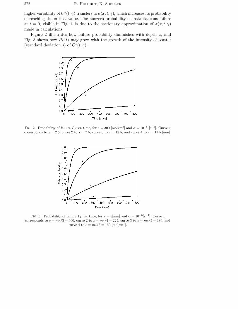
Figure 2 illustrates how failure probability diminishes with depth x, andFig. 3 shows how PF (t) may grow with the growth of the intensity of scatter(standard deviation s) of C∗(t, γ).

Fig. 2. Probability of failure PF vs. time, for s = 300 [mol/m3] and α = 10−5 [s−1]. Curve 1corresponds to x = 2.5, curve 2 to x = 7.5, curve 3 to x = 12.5, and curve 4 to x = 17.5 [mm].

Fig. 3. Probability of failure PF vs. time, for x = 5[mm] and α = 10−5[s−1]. Curve 1corresponds to s = m0/3 = 300, curve 2 to s = m0/4 = 225, curve 3 to s = m0/5 = 180, and

curve 4 to s = m0/6 = 150 [mol/m3].


The explicit dependence of failure probability on x is visualized in Fig. 4. Atpoints near the boundary, higher correlation of the values of C∗(t, γ) involveslonger expected time to failure. However, for deeper points in the half-spacethe relation turns out to be reversed, with higher correlation entailing shorterexpectation times. Thus for deeper points, the operator A is a low-pass filter:the influences of quick variations of a realization of C∗(t, γ) average out, makingfailure less probable.

Fig. 4. Expected time to failure EF vs. position x, for s = 300 [mol/m3]. Curve 1corresponds to α = 10−5, curve 2 to α = 10−5.5, curve 3 to α = 10−6, and curve 4 to

α = 10−6.5 [s−1].

4.3. Example 2. Infinite cylinder under random time-varying hydrogen action;effect on stress intensity factor

As the second example, we consider an infinite circular cylinder of radius b:B = {r = (r, θ, z) : 0 6 r 6 b} (cylindrical coordinate system is used), exposedto the action of a random hydrogen concentration C∗(t, γ) on its boundary. It isthus assumed, as in the preceding example, that C∗ varies in time but is constanton ∂B at any given moment. The initial condition for hydrogen concentrationis homogeneous: C0(r) = 0, r ∈ B, and the boundary ∂B is free of tractions,i.e. surface loading on the boundary is zero for all t. Therefore, at t = 0, thecylinder is in a stress-free state. For further stress calculations, plane state ofstrain is assumed in z direction.

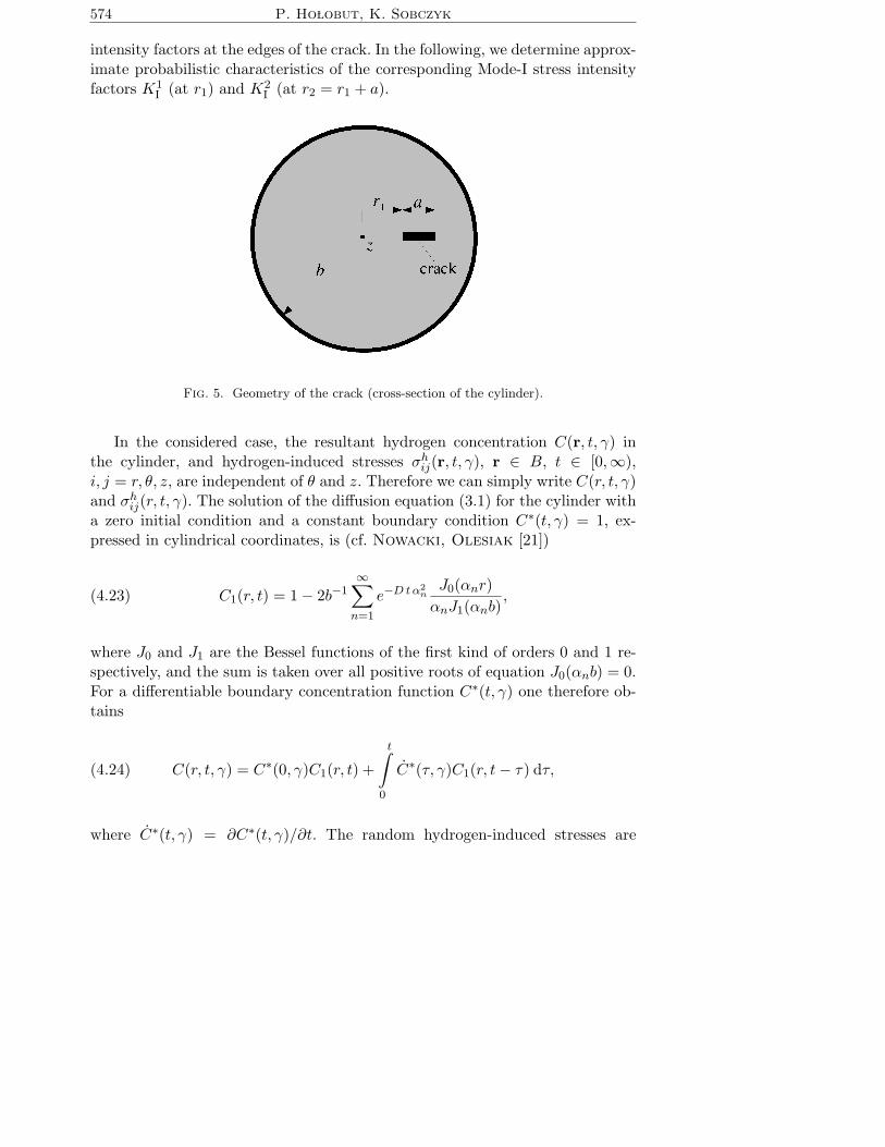
The cylinder contains a radially oriented crack of rectilinear cross-sectionand length a (Fig. 5), extended indefinitely along the z axis. As a result of theboundary hydrogen concentration C∗(t, γ), hydrogen diffuses through the cylin-der and residual stresses are induced in the material, giving rise to nonzero stress


intensity factors at the edges of the crack. In the following, we determine approx-imate probabilistic characteristics of the corresponding Mode-I stress intensityfactors K1

I (at r1) and K2I (at r2 = r1 + a).

Fig. 5. Geometry of the crack (cross-section of the cylinder).

In the considered case, the resultant hydrogen concentration C(r, t, γ) inthe cylinder, and hydrogen-induced stresses σh

ij(r, t, γ), r ∈ B, t ∈ [0,∞),i, j = r, θ, z, are independent of θ and z. Therefore we can simply write C(r, t, γ)and σh

ij(r, t, γ). The solution of the diffusion equation (3.1) for the cylinder witha zero initial condition and a constant boundary condition C∗(t, γ) = 1, ex-pressed in cylindrical coordinates, is (cf. Nowacki, Olesiak [21])

(4.23) C1(r, t) = 1 − 2b−1∞∑

n=1

e−D t α2nJ0(αnr)

αnJ1(αnb),

where J0 and J1 are the Bessel functions of the first kind of orders 0 and 1 re-spectively, and the sum is taken over all positive roots of equation J0(αnb) = 0.For a differentiable boundary concentration function C∗(t, γ) one therefore ob-tains

(4.24) C(r, t, γ) = C∗(0, γ)C1(r, t) +

t∫

0

C∗(τ, γ)C1(r, t− τ) dτ,

where C∗(t, γ) = ∂C∗(t, γ)/∂t. The random hydrogen-induced stresses are


(based on [21])

(4.25)

σrr(r, t, γ) = m

r−2

r∫

0

C(ρ, t, γ)ρ dρ− b−2

b∫

0

C(ρ, t, γ)ρ dρ

,

σθθ(r, t, γ) = m

C(r, t, γ) − r−2

r∫

0

C(ρ, t, γ)ρ dρ− b−2

b∫

0

C(ρ, t, γ)ρ dρ

,

σzz(r, t, γ) = m

C(r, t, γ) − λ

(λ+ µ)b2

b∫

0

C(ρ, t, γ)ρ dρ

.

where m = −2µβ/(λ+ 2µ). All other components of the stress tensor are zero.In the sequel, to effectively characterize the stress intensity factors K1

I and K2I ,

we make the following two simplifications. First, we disregard the multiaxialcharacter of the stress field and consider only the component σθθ which is per-pendicular to the crack surface. Second, for present considerations, we assumethe crack to be suitably small and distant from the boundary of the cylinder tobe treated as if it were placed in an infinite medium. (This second condition canbe avoided by using more specialized weight functions than we do below.) Wethus consider the crack as a rectilinear through crack in an infinite space, underuniaxial state of stress perpendicular to the crack surface. The stress intensityfactors for this case can be expressed as (based on Sih [22])

(4.26) K1I (t, γ) = R

r2∫

r1

σθθ(r, t, γ)

√r2 − r

r − r1dr,

(4.27) K2I (t, γ) = R

r2∫

r1

σθθ(r, t, γ)

√r − r1r2 − r

dr,

where R =√

2/(πa). By combining Eqs. (4.23)–(4.27), the following expressionsfor the stress intensity factors are obtained:

(4.28) KiI(t, γ) =

∞∑

n=1

Ain(ebntC∗(0, γ) + C∗

n(t, γ)) , i = 1, 2

where

A1n = R

r2∫

r1

an(r)

√r2 − r

r − r1dr , A2

n = R

r2∫

r1

an(r)

√r − r1r2 − r

dr ,


C∗n(t, γ) =

t∫

0

C∗(τ, γ) ebn(t−τ) dτ,

an(r) = − 4µβ

b(λ+ 2µ)α2n

(J1(αnr) − αnrJ0(αnr)

rJ1(αnb)+

1

b

), bn = −Dα2

n.

We next consider the case, when the boundary concentration C∗(t, γ) is givenby a stochastic parametric model (cf. Sec. 3.2.) of the particular form of a sumof deterministic base functions with random coefficients

(4.29) C∗(t, γ) =N∑

j=1

Zj(γ)fj(t).

Because of the linearity of Eqs. (4.28) in C∗(t, γ), the resultant stress intensityfactors can likewise be written as sums of deterministic functions with randomcoefficients

(4.30) KiI(t, γ) =

N∑

j=1

Zj(γ)KijI (t) , i = 1, 2

where KijI (t), i = 1, 2, are the solutions of (4.28), with fj(t) taken as the bound-

ary concentration function. The relevant probabilistic moments are easily com-puted. The mean values are

(4.31) M iI (t) = E{Ki

I(t, γ)} =N∑

j=1

MjKijI (t) , i = 1, 2

where Mj = E{Zj(γ)} is the mean of the random variable Zj(γ). The variancesare given by

(4.32) V iI (t) = E{(Ki

I(t, γ) −M iI (t))2} =

N∑

j,k=1

VjkKijI (t)Kik

I (t) , i = 1, 2

where Vjk = E{(Zj(γ) − Mj)(Zk(γ) − Mk)} is the covariance of Zj(γ) andZk(γ). In particular, when Zj(γ), j = 1, 2, . . . , N , are independent, formula(4.32) reduces to

(4.33) V iI (t) =

N∑

j=1

VjjKijI (t)

2, i = 1, 2

with Vjj being the variance of Zj(γ).


For numerical calculations we consider a cylinder of radius b = 0.1 [m] madeof low-strength steel, with material parameters as in Example 1. The crack is oflength a = 2 [mm]. The boundary concentration is assumed in the form (4.29)with N = 3 and fj(t) = sin(kjt) + 1, j = 1, 2, 3. The random variables Z1(γ),Z2(γ), Z3(γ) are independent and uniformly distributed between 0 and Z = 500[mol/m3

]. The means and variances of Zj(γ) are: Mj = Z/2 = 250

[mol/m3

]

and Vjj = Z2/12 ≈ 20833[mol2/m6

], j = 1, 2, 3. The frequencies are assumed

to have the following values: k1 = 2π/7, k2 = 2π/16, and k3 = 2π/60[day−1

].

In Figures 6 and 7 only the results for the crack edge at r1 are shown, becausethe corresponding values for the two edges differ only slightly (owing to the shortchosen crack length). It can be seen that under the action of a cyclic boundary

Fig. 6. Mean stress intensity factor at the inner edge of the crack, M1I , vs. time. Curve 1

corresponds to r1 = 78, and curve 2 to r1 = 58 [mm].

Fig. 7. Standard deviation of the stress intensity factor at the inner edge of the crack,p

V 1I

,vs. time. Curve 1 corresponds to r1 = 78, and curve 2 to r1 = 58 [mm].


concentration C∗(t, γ), the crack undergoes cyclic tension and compression (aspresented in Fig. 6 for the case of mean values). The influence of hydrogen isalso more attenuated towards the center of the cylinder: cracks closer to theboundary sustain higher stress amplitudes, and are therefore more likely topropagate. Their stress intensity factors also exhibit greater statistical scatter(Fig. 7).

5. Conclusions

In the paper, an effective method for quantitative characterization of ran-dom hydrogen-induced stresses has been presented. The method is based on therandomized diffusion-elasticity equations, but also a simpler, stochastic para-metric model, based on empirical information on hydrogen stresses, is brieflysketched. The analysis allows to perform specific calculations in a wide range ofreal situations. The numerical calculations for the examples considered providequantitative effects of random hydrogen-induced stresses on the random time tomaterial failure and on the stress intensity factors. The graphical visualizationexhibits the effects of the basic statistical characteristics of the hydrogen con-centration (e.g. its standard deviation and correlation time) on the failure timeand on the Mode-I stress intensity factor.

References

1. D. J. Unger, A mathematical analysis of impending hydrogen-assisted crack propagation,Eng. Fract. Mech., 34, 3, 657–667, 1989.

2. A. G lowacka, W. A. Swiatnicki, Effect of hydrogen charging on the microstructure of

duplex stainless steels, J. Alloys and Compounds, 356–357, 701–704, 2003.

3. P. Sofronis, R. M. McMeeking, Numerical analysis of hydrogen transport near a blunt-

ing crack tip, J. Mech. Phys. Solids, 37, 3, 317–350, 1989.

4. R. A. Oriani, P. H. Josephic, Equilibrium and kinetic studies of the hydrogen-assisted

cracking of steel, Acta Metall., 25, 979–988, 1977.

5. B. A. B. Anderson, Hydrogen-induced crack propagation in a QT-steel weldment, J. Eng.Materials and Technology, 104, 249–256, 1982.

6. J.-S. Wang, The thermodynamical aspects of hydrogen-induced embrittlement, Eng. Fract.Mech., 68, 647–669, 2001.

7. K. Sobczyk, D. J. Kirkner, Stochastic modeling of microstructures, Birkhauser, Boston,2001.

8. K. Sobczyk, Stochastic differential equations with applications to physics and engineering,Kluwer Academic Publishers, Dodrecht, 1991.

9. K. Sobczyk, J. Trebicki, A. B. Movchan, Characterization of random microstructural

stresses and fracture estimation, Eur. J. Mech. – A/Solids, 26, 4, 573–591, 2007.


10. R. B. Hetnarski, J. Ignaczak, Mathematical theory of elasticity, Taylor and Francis,New York, 2004.

11. K. Sobczyk, J. Trebicki, Fatigue crack growth in random residual stresses, Int. J. Fa-tigue, 26, 1179–1187, 2004.

12. O. Onicescu, V. I. Istratescu, Approximation theorems for random functions, Redi-conti Matem., 8, 65–81, 1975.

13. H. D. Madsen, S. Krenk, N. C. Lind, Methods of structural safety, Prentice Hall, Engle-wood Cliffs, NJ, 1986.

14. Y. K. Belayev, On the number of exits across the boundary of a region by a vector

stochastic process, Theo. Prob. Appl., 13, 320–324, 1968.

15. T. T. Soong, M. Grigoriu, Random vibration of mechanical and structural systems,Prentice Hall, 1992.

16. K. Sobczyk, B. F. Spencer, Random fatigue: from data to theory, Academic Press,Boston, 1992.

17. B. Paul, Macroscopic criteria for plastic flow and brittle fracture in Fracture: an advanced

treatise, Vol. II, H. Liebowitz, [Ed.], 313–496, Academic Press, New York, 1968.

18. T. Boellinghaus, H. Hoffmeister, A. Dangeleit, A scatterband for hydrogen diffu-

sion coefficients in micro-alloyed and low carbon structural steels, Welding in the World,35, 2, 83–96, 1995.

19. J. Hirth, Effects of hydrogen on the properties of iron and steel, Metall. Trans., 11A,861–890, 1980.

20. C. San Marchi, B. P. Somerday, S. L. Robinson, Permeability, solubility and diffusiv-

ity of hydrogen isotopes in stainless steels at high gas pressures, Int. J. Hydrogen Energy,32, 100–116, 2007.

21. W. Nowacki, Z. S. Olesiak, Termodyfuzja w cia lach sta lych (Thermo-diffusion in

solids), PWN, Warszawa, 1991 (in Polish).

22. G. C. Sih, Handbook of stress intensity factors, Institute of Fracture and Solid Mechanics,Lehigh University, Bethlehem, Pennsylvania, 1973.

Received April 26, 2007; revised version October 2, 2007.

Date post:	30-May-2020
Category:	Documents
Upload:	others
View:	20 times
Download:	0 times

Random hydrogen-induced stresses and eﬀects on cracking · Random hydrogen-induced stresses and...

Documents