Random Matrix Theory and the Electric Grid

Kate MarvelCenter for International Security and CooperationStanford University

Outline

• Complex systems: some basics

• Random Matrix Theory and nuclear physics

• Applications to complex systems

• Simple network models

• Possible extensions

The Electric Grid Generating choices in context

What is an electric grid?

• NODES: generating stations, substations of various types

• EDGES: High-voltage transmission lines

• Interested in network topology, stability.

• Very simple model- no differentiation between sources and sinks, no load.

Complex networks Some basics

Properties of complex networks

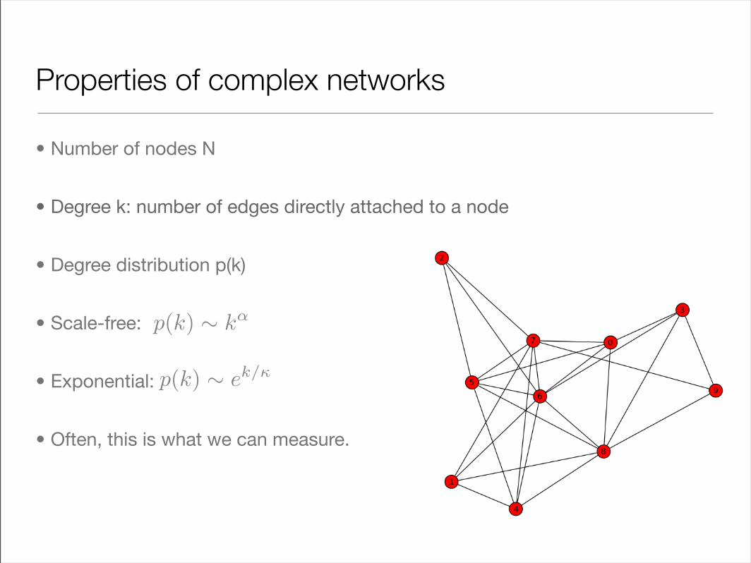
• Number of nodes N

• Degree k: number of edges directly attached to a node

• Degree distribution p(k)

• Scale-free:

• Exponential:

• Often, this is what we can measure.

p(k) ! k!

p(k) ! ek/!

Adjacency matrices

• if nodes i,j are connected by N lines

• 0 otherwise

Aij = N

[ [A B C D0 1 1 11 0 1 01 1 0 01 0 0 0

ABCD

Eigenvalues of A

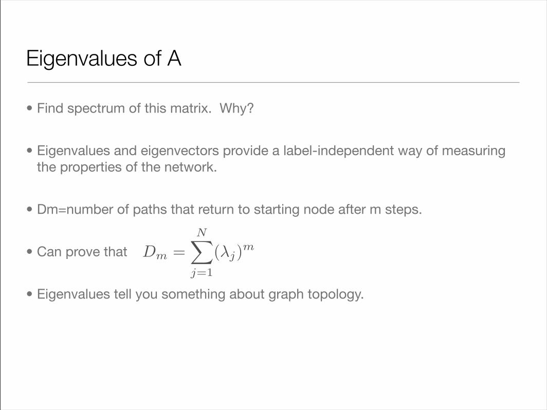
• Find spectrum of this matrix. Why?

• Eigenvalues and eigenvectors provide a label-independent way of measuring the properties of the network.

• Dm=number of paths that return to starting node after m steps.

• Can prove that

• Eigenvalues tell you something about graph topology.

Dm =N!

j=1

(!j)m

Robustness and sensitivity

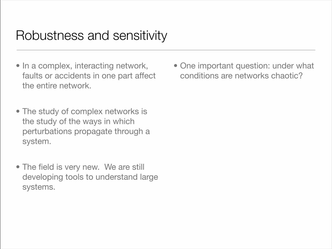
• In a complex, interacting network, faults or accidents in one part affect the entire network.

• The study of complex networks is the study of the ways in which perturbations propagate through a system.

• The field is very new. We are still developing tools to understand large systems.

• One important question: under what conditions are networks chaotic?

A short detour into nuclear physics

• Heavy nuclei are complex systems

• Interactions between nucleons are known, but in practice direct calculation is intractable.

• Need a statistical description.

• Energies of the system are eigenvalues of Hamiltonian H.

• H is a large random matrix. http://snews.bnl.gov/popsci/uranium.jpg

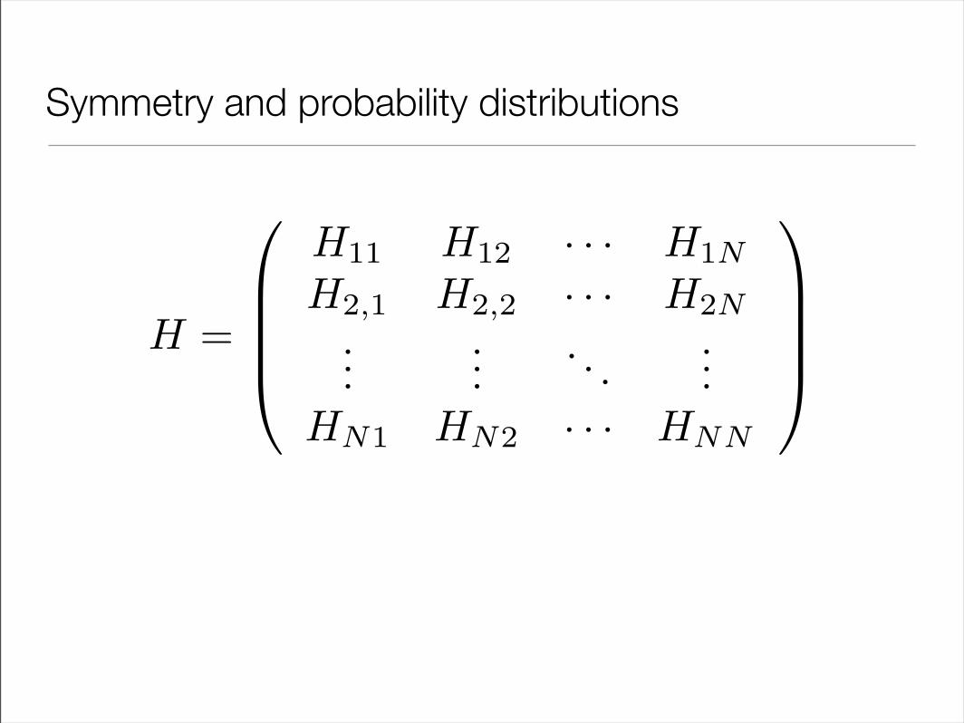
Symmetry and probability distributions

H =

!

"

"

"

#

H11 H12 · · · H1N

H2,1 H2,2 · · · H2N

.

.

.

.

.

.

...

.

.

.

HN1 HN2 · · · HNN

$

%

%

%

&

Symmetry and probability distributions

H =

!

"

"

"

#

H11 H12 · · · H1N

H2,1 H2,2 · · · H2N

.

.

.

.

.

.

...

.

.

.

HN1 HN2 · · · HNN

$

%

%

%

&

• Probability conservation:

• If time-reversal-invariant:

H = H†

H = HT

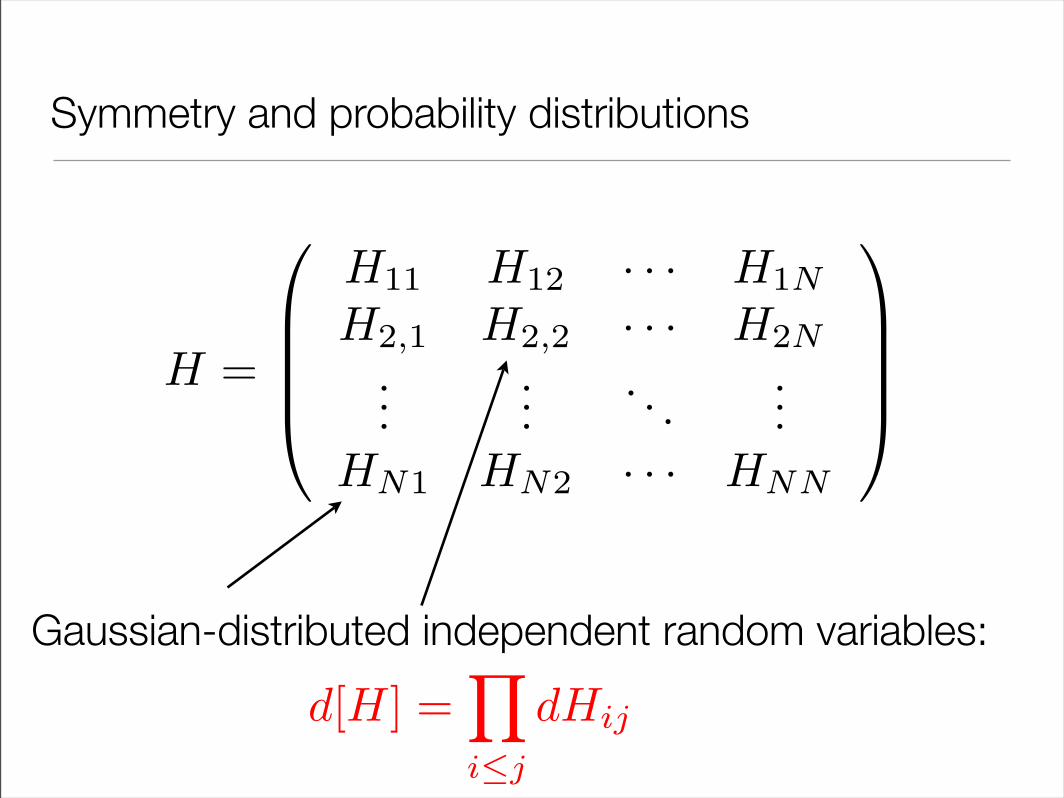
d[H] =!

i!j

dHij

Symmetry and probability distributions

H =

!

"

"

"

#

H11 H12 · · · H1N

H2,1 H2,2 · · · H2N

.

.

.

.

.

.

...

.

.

.

HN1 HN2 · · · HNN

$

%

%

%

&

Gaussian-distributed independent random variables:

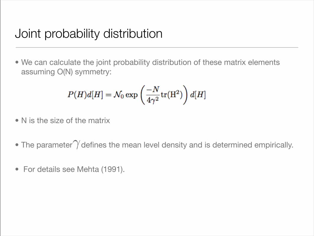
Joint probability distribution

• We can calculate the joint probability distribution of these matrix elements assuming O(N) symmetry:

• N is the size of the matrix

• The parameter defines the mean level density and is determined empirically.

• For details see Mehta (1991).

!

Gaussian Orthogonal Ensemble

• Assuming time reversal symmetry, can diagonalize H:

• So can write the probability distribution in terms of the eigenvalues:

• Define level density:

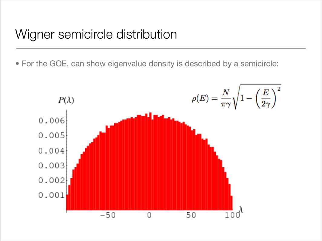
Wigner semicircle distribution

• For the GOE, can show eigenvalue density is described by a semicircle:

GOE, continued

• The symmetries of the system uniquely determine the behavior of the energy spectrum.

• The joint probability vanishes when Ei=Ej: level repulsion.

• “Unfold” spectrum so mean level spacing is one:

• Convenient to consider Nearest Neighbor Spacing Distribution:

Contrast: noninteracting system

• Here, Hamiltonian is constrained to be diagonal (no interaction terms).

• No level repulsion.

• Eigenvalues are uncorrelated random variables.

• NNSD is Poisson:

P (s) = e!s

NNSD Level repulsion vs. clustering

Gaussian Orthogonal Ensemble

Poisson

s

P(s)

NNSD Level repulsion vs. clustering

Gaussian Orthogonal Ensemble

Poisson

s

P(s)

s=0 most likely: energy levels cluster together.

NNSD Level repulsion vs. clustering

Gaussian Orthogonal Ensemble

Poisson

s

P(s)

s=0 least likely: energy levels repel each other.

Quantum Chaos Conjectures

Chaos vs. Regularity

• These distributions appear in the study of quantum chaos.

• Two main conjectures underly the field:

• Bohigas-Giannoni-Schmit: Spectra of systems whose classical analogues are fully chaotic show correlation properties consistent with the Gaussian ensembles.

• Berry-Tabor: Spectra of systems whose classical analogues are fully regular show correlation properties best described by Poisson statistics.

• Intuitively, independent variables behave in a regular way. Large correlations induce chaos.

Order to Chaos

• Real nuclear data marks integrability to chaos transition.

• Chaos here is induced by the breaking of dynamical symmetries.

• Many more degrees of freedom than conserved quantities.

• Clear Poisson to GOE transition.

Measuring intermediate distributions

• Want distribution that interpolates between GOE and Poisson.

• Brody parameter=1 for GOE, 0 for Poisson.

Back to the grid

• For a complex network, the analogue of the Hamiltonian H is the adjacency matrix A.

• Often, the only thing we can measure about a grid is its degree distribution.

• In most circumstances, this is exponential:

• Given this information, what can we say about the underlying grid statistics?

• Under what circumstances should we expect chaos?

p(k) ! e!k/!

Erdos-Renyi random graph: nodes are connected with probability p.

• Eigenvalue density for networks with varying mean degree.

• Peak at 0: nodes with connectivity 1 interacting with highly connected node.

• Peaks at +=1: connected pairs disconnected from greater network.

• Peaks decrease with increasing mean degree.

Exponential distributions

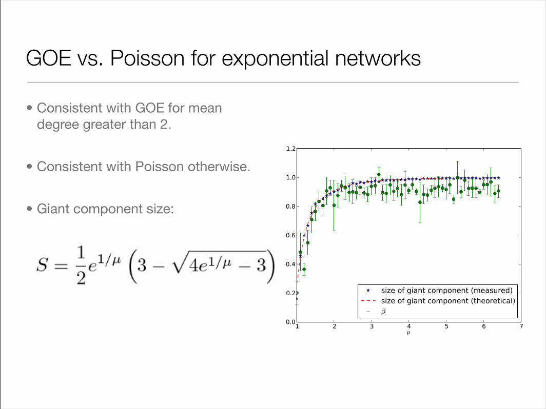
GOE vs. Poisson for exponential networks

• Consistent with GOE for mean degree greater than 2.

• Consistent with Poisson otherwise.

• Giant component size:

Linking networks: superposition

• Consider two copies of the same network. If they are completely disconnected, their NNSD should be given by superposed GOEs:

Connecting with a single edge

• Linking the two networks with a single edge produces a strange distribution.

Describing interconnection

• In the absence of connections between networks, adjacency matrix is block diagonal:

• Connections add off-diagonal elements:

•

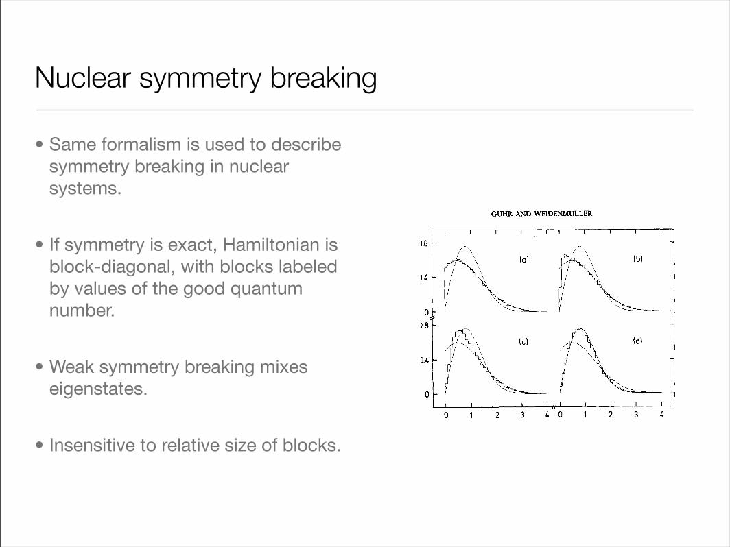
Nuclear symmetry breaking

• Same formalism is used to describe symmetry breaking in nuclear systems.

• If symmetry is exact, Hamiltonian is block-diagonal, with blocks labeled by values of the good quantum number.

• Weak symmetry breaking mixes eigenstates.

• Insensitive to relative size of blocks.

422

0.8

0 p ISI

0.8

GUHR AND WEIDENMijLLER

I I I I I ,

P 012 3 LO 3 s

FIG. 3.1. Numerically simulated spacing distributions p(s) in case I, plotted as histograms. The values of the mixing parameter G( correspond to the labels (a) to (d) in Table I. The theoretical spacing distributions for a single GOE and a non-interacting superposition according to Eq. (2.2) with equal level densities are plotted as solid lines.

0.e

0.1

C plsl

0.E

0.1

0

I I I I I I I I I I

I I I I I ,rI I I I I

012 3 1012 3 L

S

FIG. 3.2. Numerically simulated spacing distributions p(s) in case II, plotted as histograms. The values of the mixing parameter a. correspond to the labels (a) to (d) in Table I. The theoretical spacing distributions for a single GOE and a non-interacting superposition according to Eq. (2.2) with fractional level densities g, = f and g, = f are plotted as solid lines.

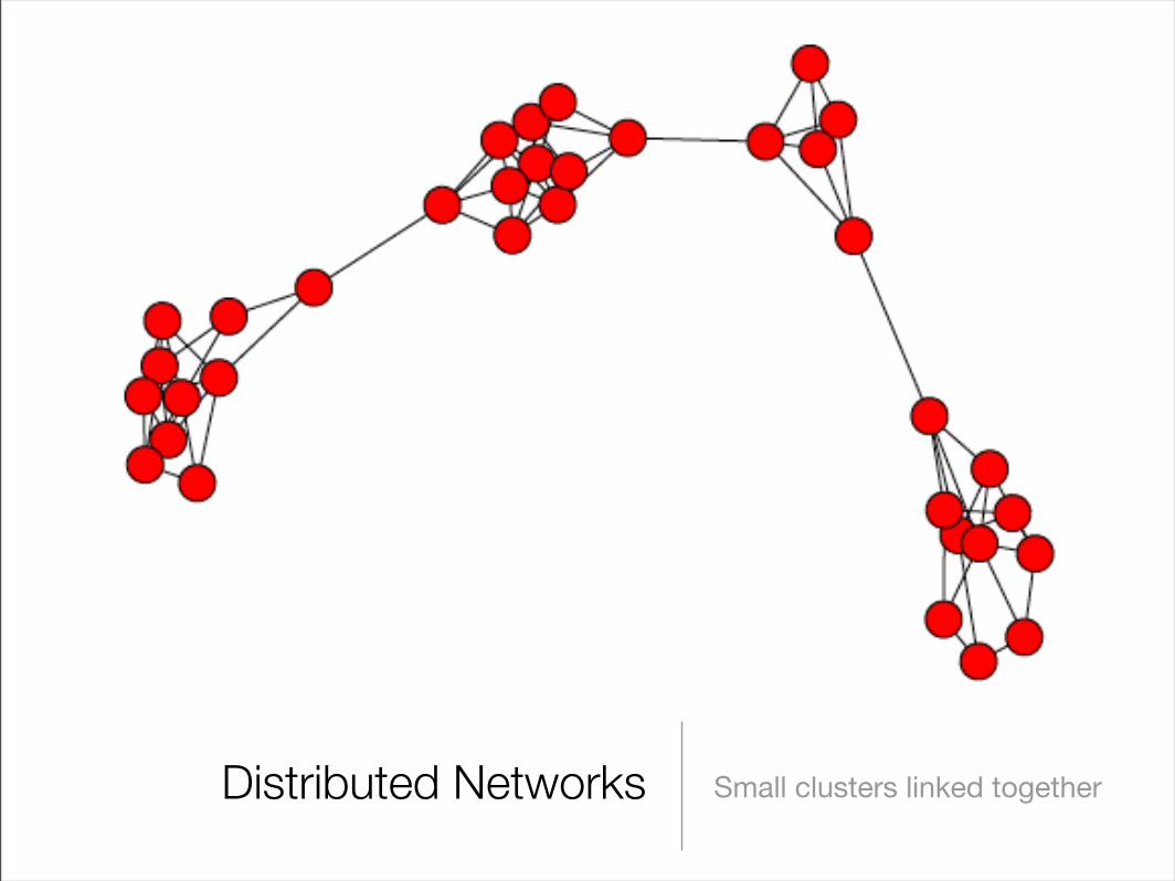
Distributed Networks Small clusters linked together

Distributed networks

• Model by linking m identical regions of equal size N.

• I=number of interconnectors. For I/N <<<1, get Poisson statistics for m of order N/100.

• However, for sufficiently large I/N, retain GOE distribution even for m of order N.

• Within each region, eigenvalues highly correlated, so any fault or fluctuation propagates through entire region.

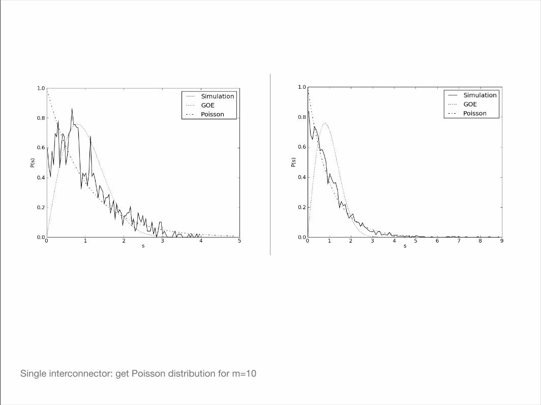
Single interconnector: get Poisson distribution for m=10

I=2: do not get Poisson distribution even for m=50.

Conclusions

• Grids matter. They provide context and help us to ask the right questions.

• Surprising tools from nuclear physics can help us understand the connectivity and correlation properties of large complex systems.

• The NNSD helps to illustrate correlations between nodes in a system and provides insight into how failures and fluctuations propagate.

• More work is needed to incorporate network topology information with existing load flow models.

• Controlling chaos through strategic load management?