1 / 84

Random ProcessesSimulation and Modeling (CSCI 3010U)

Faisal Qureshihttp://vclab.science.uoit.ca

Computer Science, Faculty of Science

2 / 84

Figure 1: Dilbert and randomness

3 / 84

Random ProcessesI Simulate random processes or activitiesI Approximate phenomena that are too hard to describe

deterministically, or a deterministic simulation is too costlyI Provide variation in the simulation data, so we can estimate

errors or compute the range of an output

4 / 84

Monte Carlo SimulationsI Using repeated sampling to determine the properties of some

phenomenonI Principle of inferential statistics

I A random sample tends to exhibit the same properties as thepopulation from which it is drawn from

I This principle doesn’t always hold, which can lead to inaccurateresults

ExampleWhat is the probability of not getting a single head after 10 coinflips?

5 / 84

Monte Carlo SimulationsWhat is the probability of getting a boxcars in a game of craps after24 throws?

I Solve analyticallyI Compute by writing a program

6 / 84

How many trials?Law of Large NumbersIn repeated independent tests with some actual probability p of anoutcome for each test, the chance that the fraction of time thatoutcome occurs converges to p as the number of trials goes toinfinity

Gambler’s FallacyI Say you flip a coin 10 times, and get a string of heads. Are we

more likely to get a head the 11th time?I No

7 / 84

How many trials?How many samples are needed to have confidence in results?

Notion of VarianceHow much spread there is in the possible outcomes

Standard deviationThe fraction of values taht are close to the mean

σ(x) =√√√√ 1|X|

∑x∈X

(x− µ)2

I µ is the meanI |X| is cardinality of x

8 / 84

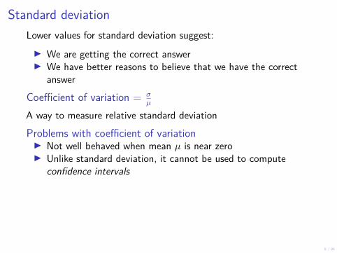
Standard deviationLower values for standard deviation suggest:

I We are getting the correct answerI We have better reasons to believe that we have the correct

answer

Coefficient of variation = σµ

A way to measure relative standard deviation

Problems with coefficient of variationI Not well behaved when mean µ is near zeroI Unlike standard deviation, it cannot be used to compute

confidence intervals

9 / 84

Confidence IntervalsEstimate the unknown parameters by providing a range thatcontains unknown value and a confidence level that the unknown liewithin that range

ExampleA candidate is expected to get 75% plus-minus 4% votesUnstated assumptionsI Confidence level is 5%I Elections are random trials that have normal distributions

10 / 84

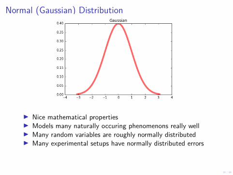
Normal (Gaussian) Distribution

I Nice mathematical propertiesI Models many naturally occuring phenomenons really wellI Many random variables are roughly normally distributedI Many experimental setups have normally distributed errors

11 / 84

Normal Distribution and Confidence IntervalsI Normal distribution is characterized by mean and varianceI Mean and variance can be used to construct confidence

intervals

I 68% of data within 1 standard deviation of meanI 95% of data within 2 standard devication of meanI 99.7% of data within 3 standard devication of mean

12 / 84

Nuclear DecayConsider a large number of radioactive nuclei. According to the lawof radioactive decay, the rate of decay is proportional to the numberof nuclei. We can express this as the following differential equation:

dN

dt= −λN.

Here, N is the number of nuclei and λ is the decay constant.

13 / 84

Nuclear Decay - Analytical SolutionWe can actually solve this equation analytically and determine thenumber of nuclei remaining after time t

N(t) = N(0)e−λt.

I N(0) is the initial number of nuclei.I N(t) is the number of nuclei remaining after time t.

14 / 84

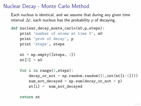
Nuclear Decay - Monte Carlo MethodEach nucleus is identical, and we assume that during any given timeinterval ∆t, each nucleus has the probability p of decaying.

def nuclear_decay_monte_carlo(n0,p,steps):print 'number of atoms at time 0', n0print 'prob of decay', pprint 'steps', steps

nt = np.empty([steps, 1])nt[0] = n0

for i in range(1,steps):decay_or_not = np.random.random((1,int(nt[i-1])))num_not_decayed = np.sum(decay_or_not > p)nt[i] = num_not_decayed

return nt

15 / 84

Nuclear Decay

16 / 84

Random WalksIn 1D random walk, the walker starts at origin and takes a rightstep with probability p and left step with probability 1− p.

n = 1000x(0) = 0do:

n -= nc = draw_a_random_number()if c < p:

x(t+1) = x(t) + 1else:

x(t+1) = x(t) - 1while n > 0

The walk takes one step in each time step of the simulation.

17 / 84

Multi-dimensional random walksIt is straightforward to extend a random walk to higher dimensions.

Example: 2D random walk

A walker takes one of up, down, left or right steps based upon theassociated probabilities: pu, pd, pl and pr. These probabilities allsum to 1.

18 / 84

Collecting statistics from random walksTo get anything meaningful out of such simulations, we need torepeat them many times and collect statistics.

I Mean distance, what is the mean position of the walker afterN steps.

I Maximum distance, what is the maximum distance that awalker reached during one of the runs.

I Average maximum distance, what is the average maximumdistance that walker reached during all the runs.

I Histogram of positions

19 / 84

Random step lengthsI Changing step size at each time stepI Step size can also be a function of the length of the walk

I Either growing or shrinking as the walks get longerI Different step sizes in different directions

20 / 84

Boundary conditions 1What if the space is limited and the random walk hits a boundary?

I Absorbing boundary, walker is consumed upon hitting theboundary.

I Reflecting boundary, walker changes direction upon hitting theboundary.

I Periodic boundary, walker appears at the positive boundaryafter passing through the negative boundary and vice versa.I Often used to simulated circular domains.

I Random boundary, walker is placed at a random location eachtime it hits the boundary.

21 / 84

Boundary conditions 2Absorbing boundary conditionsI With absorbing boundary conditions the walks can end earlyI This creates significant challenges when collecting statistics

Reflecting boundary conditionsI Walker tends to stay at the edges of the region

22 / 84

Boundary conditions 3Periodic boundary conditionsI Periodic boundary conditions produce a more uniform

distributionI This is easily explained, since walkers do not stick to the edges

Random boundary conditionsI Creates uniform trails (distribution over locations)

23 / 84

Random walks: are they truly that random?Some aspects of random works are surprising in the sense that theseare not random at all.

I E.g., even length random walks (with step size of 1) all end upat even locations.

I E.g., odd length random walks (with step size of 1) all end upat odd locations.

We can introduce randomness by exploiting boundary conditions.

24 / 84

Variations on random walks 1TrapsTrap is an extension of absorbing boundary condition. Here trapsare randomly placed all over the region. A walker is consumed uponreaching a trap. Optionally it is possible to randomly place thewalker at a different location in the region.Absorbing boundary conditions and traps can often lead to veryshort walks.I One option is to create a new walker (usually at a random

location) whenever a walker dies.I Second option is to have more than one walkers in parallel. If

there are large enough walkers, the chances are high that someof these will survive longer than others.

25 / 84

Variations on random walks 2When multiple walkers are active at the same time, it raises thespectre of collisions between walkers.

I Ignore the collisionsI Kill off one of the walkerI Walkers transform each other upon collision

I This is often used when simulating chemical reactions

26 / 84

Applications of random walks

27 / 84

Solving the diffusion equationConsider the diffusion equation

∂P (x, t)∂t

= D∂2P (x, t)∂x2

It is used to model a variety of physical processes, including fluidflow. It is also used in finance. Analytical solutions to diffusionequation do not exist except for the simplest cases. A suite ofnumerical solutions have been proposed in the literature. Numericalsolutions, however, cannot be easily parallelized. Furthermore, thesecan only be used for a small set of boundary conditions.

28 / 84

Solving the diffusion equationIt turns out that we can use random walks to solve the diffusionequation. Asymptotically as the number of walks approach infinity,the average properties of a random walk approach the solution to adiffusion equation.

Insight

I We are essentially replacing human time with computer time.Instead of coming up with a numerical or analytical solution tothe problem, we will let computer figure it by running millionsand millions of random walks.

I It is easy to model boundary conditions in random walks.I Random walks can easily exploit multiple processors.

29 / 84

Modeling a rain drop falling in strong wind

30 / 84

Variations on random walksPersistent random walksProbabilities for the current step depends upon the previous step.

Multi-state random walksThe random walk can be in one of multiple states, which determinethe probabilities for the current step.This is akin to having a finite state machine with random transitions.

31 / 84

An application of multi-state random walksChromatographic columnsOne application of multi-state walks is diffusion in achromatographic column. In this application we are interested inhow far a particular compound will move along a chromatographiccolumn in a certain length of time. For each type of compound wehave a probability α that it will move v units in each time step anda probability 1− α that it will not move.

32 / 84

Self avoiding random walksI A SAW is a random walk on a 2D or 3D lattice that cannot

return to one of the lattice points that it has already visitedI SAWs are of interest in several areas of physics and

mathematics, and surprisingly a number of their propertieshave resisted rigorous mathematical analysis, so they must bestudied in simulation

I SAWs terminate quicklyI Consider a 2D lattice, a random walk with up, down, left, right

step has a 3.7% chance of finishing just after 4 stepsI How do we generate walks of lengths more than 1000?

33 / 84

Self avoiding random walksI Adjust statistics to account for a less random selection

I If one of the three moves is blocked, we can still randomlyselect one of the two open moves, but giving less weight to thestatistics computed for this walk

Computing weight w(N) for a walk of length NI w(1) = 1, since we can always take the first stepI If all three moves are blocked w(N) = 0I If all three moves are possible w(N) = w(N − 1)I If only m moves are possible, 0 < m < 3, thenw(N) = m

3 w(N − 1), select one of the m possible moves atrandom

Combining statistics over many walks

⟨R2⟩

=∑iwi(N)R2

i∑iwi(N)

34 / 84

Self avoiding random walksI The strategy described in the previous slide gives us longer

walks, since we are able to avoid some terminationsI Walks with heigher weights are in a way healthier, we can make

more copies of theseI Compute ri = w(N)

〈w(N)〉 . For a healthy walk, ri > 1.I If ri > 1, make c copies of the walker and assign each of the

walkers weight w(N)c

I The number of copies is given by c = min(ri,m), where m isthe possible number of moves

I If ri < 1 then the walker is removed with probability 1− ri

35 / 84

Applications of self avoiding random walksPolymer physicsI A polymer consists of N repeated units, called monomers.I Each monomer consists of a small number of tightly bound

atoms. Typically N is in the 103 to 105 range.I For polymers of length N one of the important physical

properties is⟨R2N

⟩, the mean squared end-to-end length of the

polymer

(From U. Reading, UK)

36 / 84

Random numbersThere are ways to generate truly random numbers, but these requirephysical processes, those that we believe to be truly random.

I Physical processes are costly and there isn’t an easy way tointerface these with a computer.

I Physical process are not repeatable, so we can’t use the sameset of random numbers in several simulations for testing andcomparison. (Of course we can always save the randomnumbers.)

37 / 84

Pseudo random numbersPseudo random numbers are generated using deterministictechniques, but they appear to be random

We can always reproduce the same set of random numbers by usingthe same starting conditions

We can also analyze them mathematically i.e. these numbers havethe same statistical properties as “truly” random numbers

38 / 84

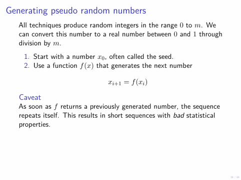
Generating pseudo random numbersAll techniques produce random integers in the range 0 to m. Wecan convert this number to a real number between 0 and 1 throughdivision by m.

1. Start with a number x0, often called the seed.2. Use a function f(x) that generates the next number

xi+1 = f(xi)

CaveatAs soon as f returns a previously generated number, the sequencerepeats itself. This results in short sequences with bad statisticalproperties.

39 / 84

Generating uniformly distributed random numbersI Simplest type of random number generatorI Easy to analyzeI Good random number generators exist

It is possible to generate random numbers from otherdistributions given uniformly distributed random numbers.

40 / 84

Linear Congruential Method (LCM)One of the best random number generator is also the simplest

xi+1 = (axi + c) mod m,

where

I m, the modulus, m > 0.I a, the multiplier, 0 < a < m.I c, the increment, 0 ≤ c < m.I x0, the starting value, 0 ≤ x0 < m.

Python code for LCMdef lcm(m, a, c, seed):

while True:seed = (a * seed + c) % myield seed

41 / 84

Linear congruential methodI The quality of the random number generator depends heavily

on the choice of m, a and cI The length of the sequence cannot exceed m, since there are

only m values less than m, so we want m to be as large aspossible

I Good values of a and c depend upon the value of mI Rubric:

I c is relatively prime to mI b = a− 1 is a multiple of p, for prime p dividing mI b is a multiple of 4, if m is a multiple of 4

42 / 84

Linear congruential methodLCM has been studied extensively for 50 years or so, and goodvalues for a, c and m are available.

! " #134456 8121 28411

243000 4561 51349

259200 7141 54773

233280 9301 49297

714025 4096 150889

Figure 2: LCM Values

43 / 84

Generating longer random number sequencesIn many simulations we often need billions of random numbers. Sohow can we generate longer sequences. Recall LCM can onlyproduce sequences of length less than or equal to m.

The length of the sequence (after which the sequence repeats itself)is called the period of the random number generator.

Shuffling techniqueThe range of an LCM can be increased using a shuffling technique.

44 / 84

Shuffling techniqueProcedure1. Initialize k entries of array v with random values between 0 and

1.2. Generate a random number y between 0 and m3. Compute index j = k y

m4. Set r = v[j]5. Generate a random number y between 0 and m6. Set v[j] = y7. Returns r

PropertiesI If m is the sequence length produced by the base random

number generator then shuffling will produce a sequence that isseveral times m in length.

I Shuffling also reduces any correlations that might exist in theoriginal sequence.

45 / 84

Correlations

corr(X,Y ) = cov(X,Y )σXσY

= E[(X − µX)(Y − µY )]σXσY

46 / 84

Tests for random numbersGeneral tests for randomness that can be used for any distributions

I Chi-square testI Kolmogorov-Smirnov test

47 / 84

Chi-square testI A statistical test commonly used to compare observed data

with data one would expect to obtain according to a specifichypothesis

I Chi-square test accepts or rejects the Null Hypothesis, whichstates that there is no statistically significant differencebetween the observed and the expected frequencies

48 / 84

Using Chi-square test for testing the Null HypothesisI Compute χ2 statistic as follows

χ2 =∑i

(Oi − Ei)2

Ei,

where Oi is the observed count in bin i and Ei is the expectedcount in bin i

I Compute degrees of freedom as follows

d = #bins− 1

I Use χ2 and d to compute p-value as follows:

p-value = P (X > χ2(d))

I If p-value is less than then the level of significance (usually0.05), reject the Null Hypothesis.

49 / 84

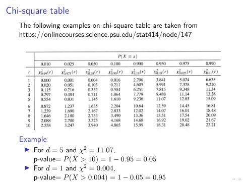
Chi-square tableThe following examples on chi-square table are taken fromhttps://onlinecourses.science.psu.edu/stat414/node/147

ExampleI For d = 5 and χ2 = 11.07,

p-value= P (X > 10) = 1− 0.95 = 0.05I For d = 1 and χ2 = 0.004,

p-value= P (X > 0.004) = 1− 0.05 = 0.95

50 / 84

Chi square test: p-values and α-valuesI A p-value is used in hypothesis testing. The smaller the

p-value, the stronger the evidence that you should reject thenull hypothesis.I p-value > 0.10: No evidence against the null hypothesis. The

data appear to be consistent with the null hypothesis.I 0.05 < p-value < 0.10: Weak evidence against the null

hypothesis in favor of the alternative.I 0.01 < p-value < 0.05: Moderate evidence against the null

hypothesis in favor of the alternative.I 0.001 < p-value < 0.01: Strong evidence against the null

hypothesis in favor of the alternative.I p-value < 0.001 Very strong evidence against the null

hypothesis in favour of the alternativeI Significance level is a measure of how certain you want to be

about your results: low significance values correspond to a lowprobability that the experimental results happened by chance.I Scientists usually set the significance level at 0.05, or 5 percent.

This means that experimental results have, at most, a 5%chance of being reproduced in a random sampling process.

51 / 84

Apply Chi-square test to see if a coin is biasedSay we flipped a coin 51 times, and we got 28 heads and 23 tails.These are observed frequences. The expected number of heads andtails for an unbiased coin, after 51 flips, is 25.5.

χ2 = (28− 25.5)2

25.5 + (23− 25.5)2

25.5= 0.516

Since for this experiment the number of outcomes is 2 (head or tail),the degree of freedom is 2− 1 = 1. Using the table above we seethat the p-value is between 0.9 and 0.1 (corresponding theχ2expected) values of 0.016 and 2.706. Consequently p-value is

greater than the level of significance, which we choose to be 0.05.We accept the Null Hypothesis.

The coin is not biased.

52 / 84

Chi-square test for uniform random number generatorGiven Yi the number of items in bin i, and pi the probability that anitem is placed in bin i, we compute Chi-Square statistics as follows:

χ2 =k∑i=1

(Yi − npi)2

npi,

where n is the number of items and k is the number of bins.

In the case of uniform random number generator, we expect thatthe probability of falling in a bin is equally likely, i.e., pi = 1/k.

Apply the Chi square test with degree of freedom = k − 1

53 / 84

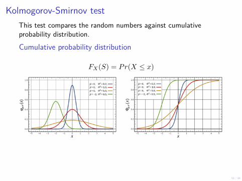
Kolmogorov-Smirnov testThis test compares the random numbers against cumulativeprobability distribution.

Cumulative probability distribution

FX(S) = Pr(X ≤ x)

54 / 84

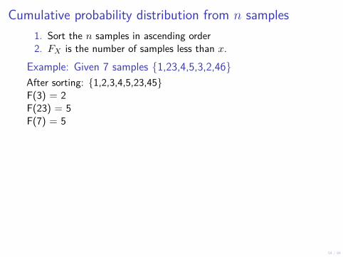
Cumulative probability distribution from n samples1. Sort the n samples in ascending order2. FX is the number of samples less than x.

Example: Given 7 samples {1,23,4,5,3,2,46}After sorting: {1,2,3,4,5,23,45}F(3) = 2F(23) = 5F(7) = 5

55 / 84

Kolmogorov-Smirnov testI A statistical hypothesis testI KS is non-parametric and entirely agnosticI KS checks the null hypothesis, which states that the sample is

taken from the “expected” distribution

56 / 84

Kolmogorov-Smirnov testI Compute cumulative probability distribution from the sampleI Compute the distance between the sample cumulative

probability distribution and the desired cumulative probabilitydistributionI Let D be the maximum of these distances.

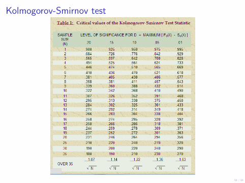
I Compute Dcritical (See table in the next slides)I If D < Dcritical then the null hypothesis holds

57 / 84

Applying Kolmogorov-Smirnov test to check if thefollowing numbers are sampled from a normal distribution

I Sampled numbers: 0.15, 0.94, 0.05, 0.51, 0.29I Dcritical = .565 We find this value in the KS Test Statistic

Table (for 0.05 significance and for 5 samples) seen in the nextslide

I Compute D (exercise)I If D < Dcritical the null-hypothesis holds, meaning the

sampled numbers come from a normal distribution

58 / 84

Kolmogorov-Smirnov test

59 / 84

Tests for uniformly distributed random numbersI Equidistribution testI Serial testI Coupon collecter’s testI Serial correlation test

60 / 84

Equidistribution testThe equidistribution test is based on the fact that uniform randomintegers should be evenly distributed amongst the possible integervalues

1. Chose some convenient d (not too large) and then generate asequence of random integers between 0 and d− 1

2. Assign them to d bins based on their integer values (since thenumbers are uniformly distributed we would expect to find anequal number of integers in each bin)

3. With a sequence of n numbers, we would expect to find nd

integers in each bin, so we can use a Chi-square test. In thiscase we have pi = 1

d , and the number of degrees of freedom isd− 1

4. Use Chi-square test

61 / 84

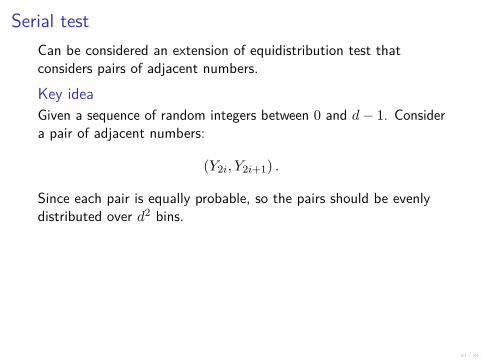
Serial testCan be considered an extension of equidistribution test thatconsiders pairs of adjacent numbers.

Key ideaGiven a sequence of random integers between 0 and d− 1. Considera pair of adjacent numbers:

(Y2i, Y2i+1) .

Since each pair is equally probable, so the pairs should be evenlydistributed over d2 bins.

62 / 84

Serial test1. Generate a sequence of n random integers2. Divide the sequence into n

2 pairs.3. Each pair is assigned to one of the d2 bins.4. Apply Chi-square test. Probability for each bin is 1

d2 and thedegrees of freedom is d2.

CaveatI For this to work the sequence should be reasonable long (the

length should be at least 5d2).I This approach can be extended to higher dimensions. However,

it quickly becomes infeasible since the number of bins growvery rapidly.

I Not practical beyond quadruples of random numbers.

63 / 84

Coupon collector’s testI This test is also based on a sequence of integer random

numbers between 0 and d− 1, but now we are interested incollecting a complete set of integers between 0 and d− 1, haveat least one of each

I In particular we are interested in the length of sequence r thatit takes to get the complete set

ProcedureI We start at the beginning of the sequence and keeping moving

down the sequence until we find a complete set of d integersI The position where this occurs is called the sequence length

I We then move to the next item in the sequence and repeat theprocess

I We are interested in the distribution of sequence lengths

64 / 84

Coupon collector’s testI The following experession gives probabilities for sequences of

lengths n ≥ 10

pn = 110n−1

q∑j=0

(−1)j(qj

)(q − j)n−1

I Use Chi-Square test to see if the observed sequence lengthsmatch those returned by the above expression

65 / 84

Spectral testI One of the best tests for random number generators is the

Spectral testI This test can only be applied to linear congruential random

number generatorsI So far all random number generators that are known to be

good pass this test, and all that are known to be bad fail itI This test is quite complicated, so we won’t examine the details,

only the basic ideasI The test operates on the real random numbers sequence and it

examines all m numbers in the sequenceI The test starts by constructing t dimensional points out of the

sequence of random numbers. We construct m points asfollows:

(Un, Un+1, Un+2, · · · , Un+t−1)I A new point is constructed starting from each number, so each

number in the original sequence appears in t points.

Generally speaking t is between 2 and 6.

66 / 84

Spectral test

I Notice the pattern observed in the above figureI “Real” random numbers when truncted exhibit the same

patternI Grain of the random number generator

67 / 84

A note about the quality of random number generatorsI These tests are applied to different sequences generated by a

random number generatorI All sequences from a “good” generator will pass these testsI In practice, however, some sequences even from a “good”

generator will fail some testsI This behavior is also observed for “true” random number

sequences

68 / 84

Generating random numbers from uniform distributionsGiven: uniform random number generator that return an integer Ubetween 0 and d.

Recipe to get a uniform random number r between a and b.

r = a+ (b− a)Ud

Recipe to get a uniform random number r between 0 and 1.

r = U

d

69 / 84

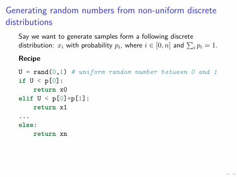
Generating random numbers from non-uniform discretedistributions

Say we want to generate samples form a following discretedistribution: xi with probability pi, where i ∈ [0, n] and

∑i pi = 1.

Recipe

U = rand(0,1) # uniform random number between 0 and 1if U < p[0]:

return x0elif U < p[0]+p[1]:

return x1...else:

return xn

70 / 84

Generating random numbers from non-uniform discretedistributions

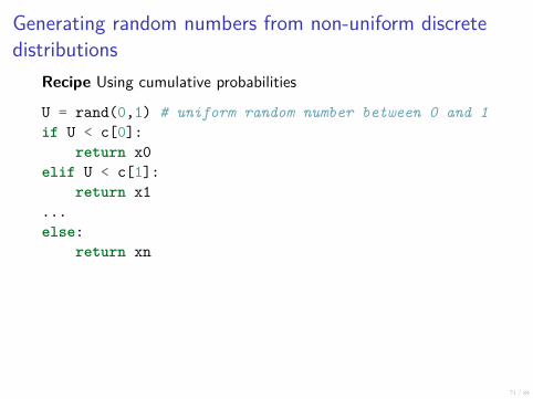
We can also store the cumulative probabilities, so we don’t have tocompute probability sums eachtime as follows:

cj =j∑i=0

pi,

where j ∈ [0, n].

Always keep the most likely choices (those with higher probabilities)at the top. This saves a lot of “if” comparisons. Also allows us touse binary search to find the correct bin.

71 / 84

Generating random numbers from non-uniform discretedistributions

Recipe Using cumulative probabilities

U = rand(0,1) # uniform random number between 0 and 1if U < c[0]:

return x0elif U < c[1]:

return x1...else:

return xn

72 / 84

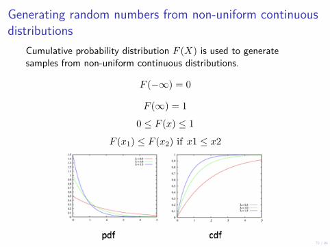
Generating random numbers from non-uniform continuousdistributions

Cumulative probability distribution F (X) is used to generatesamples from non-uniform continuous distributions.

F (−∞) = 0

F (∞) = 1

0 ≤ F (x) ≤ 1

F (x1) ≤ F (x2) if x1 ≤ x2

73 / 84

Generating random numbers from non-uniform continuousdistributions

Consider the cumulative probability distributionF (X) = Pr(x ≤ X) (associated with probability distribution f(x),where x is the random variable with distribution f(x)).

Insight

A uniform random number generator produces a random probabilityand the value of F (X) is a probability, so the inverse of F (X) takesthe probability and returns a random number with probability f(X).

74 / 84

Generating random numbers from non-uniform continuousdistributions

Given F (X) = Pr(x ≤ X) (associated with probability distributionf(x), where x is the random variable with distribution f(x)).

If F−1(X) then it is straightforward to get a random number fromf(x) using the following recipe.

u = rand(0,1) # a uniform random number between 0 and 1

return F_inv(u)

The key challenge is that in many cases F−1 doesn’t exist.

75 / 84

Generating random numbers from exponential distributionsExponential distributions, for example is used in nuclear decay — ifa substance emits a particle every µ seconds on average, then thetimes between two emissions will be exponentially distributed withmean µ.

Cumulative probability distribution for exponential distribution is

F (x) = 1− e−xµ

.

76 / 84

Generating random numbers from exponential distributionsF−1(x) for cumulative probability distribution for exponentialdistribution is

F−1(x) = −µ ln(1− U)

ln is slow; however, this approach is acceptable unless we plan togenerate a very large number of samples.

77 / 84

Generating samples from normal distributionOne of the most used probability distribution

78 / 84

Generating samples from normal distributionWe will focus on generating samples form normal distribution ofmean (µ) 0 and variance (σ2) 1.

It is easy to generate samples from normal distribution N(µ, σ) asfollows:

1. n ∼ N(0, 1) (a random number generated from a uniformdistribution with mean 0 and variance 1)

2. µ+ σn ∼ N(µ, σ)

79 / 84

Generating samples from normal distributionCumulative probability distribution for N(0, 1) is

F (x) = 1√2π

∫ ∞−∞

e−t22 dt

In this case it is F (x) is invertible; however, it is not easy tocompute.

We will look at two other approaches (for generating numbers fromnormal distribution) that give acceptable results.

80 / 84

Generating samples from normal distributionWe will use the rejection method to generate samples from a normaldistribution

Rejection method

1. Generate a sample and check to see if it is from the desireddistribution.

2. If yes, return the sample.3. Else, try again.

The trick is to guess the correct samples more frequently, to avoidhaving to generate many samples.

81 / 84

Polar method for generating samples from normaldistribution

1. Generate two uniform random numbers U1 and U22. Set V1 = 2U1 − 1 and V2 = 2U2 − 13. Compute S = V 2

1 + V 22

4. If S ≥ 1 return to step 15. Else compute

X1 = V1

√−2 lnSS

and

X2 = V2

√−2 lnSS

6. Return X1 and X2

82 / 84

Polar method for generating samples from normaldistribution

I This method produces two samplesI The downside is that the method uses logarithm and square

root operations, which are expensiveI The polar method needs a random point (V1, V2) distributed

on a circle with radius 1. This is hard to generate, but it iseasy to generate a random point within a square. So we usethe smallest square containing the circle and generate arandom point within this square. If this point is also within thecircle we continue, otherwise we generate another point.

83 / 84

Ratio method for generating samples from normaldistribution

1. Generate two uniform random numbers U1 and U2

2. Set X =√

82e

(U2− 12 )

U1

3. If X2 ≤ 5− 4e14U1 return X

4. If X2 ≥ 5− 4e−1.35U1 + 1.4 go back to step 15. If X2 ≤ − 4

lnU1return X

6. Go back to step 1

Steps 2 and 3 are optional, but they increase the efficiency of thealgorithm considerably. In this case we only produce one randomnumber, but we avoid using logarithm most of the time, so it couldbe more efficient than the polar method. Again we generate a pairof random numbers, and then check to see if they produce the rightresult, otherwise we try again.

84 / 84

SummaryI Monte Carlo techniquesI Random walksI Techniques for generating and testing sequences of random

numbersI Applications of random walks