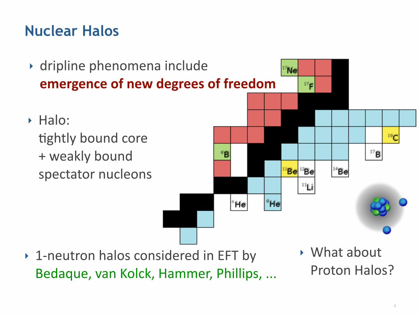
Range corrections in proton halo nuclei Lucas Pla)er Department of Physics & Astronomy University of Tennessee, Knoxville & Oak Ridge NaDonal Laboratory Collaborators: B. Acharya, E. Braaten, B. Carlsson, C. Forssén, H.-W. Hammer, C. Ji, D. Phillips, E. Ryberg
Outline Introduction Halo e�ective field theory S-wave proton halos in EFT The 8B proton halo in EFT Outlook Summary
Charge form factor
The LO loop diagrams
+
• LO diagrams, with a virtual photon leg.
i�0LO(Q) = ieZcore
⌅d3r(0|GC(�B)|r) exp (ifQ · r)(r|GC(�B)|0)
+⇧(f ⇤ 1� f ), (Zcore ⇤ 1)
⌃
• Only the S-wave part of (0|GC |r) contributes.
⌅rLOC ⇧2 = �⇥6⇥kCm2
R
+O(�2/k2C)
⇤6
e(Zcore + 1)�0LO
���Q2
⇥ (0.59 fm)2
E. Ryberg
Outline Introduction Halo e�ective field theory S-wave proton halos in EFT The 8B proton halo in EFT Outlook Summary
Charge form factor
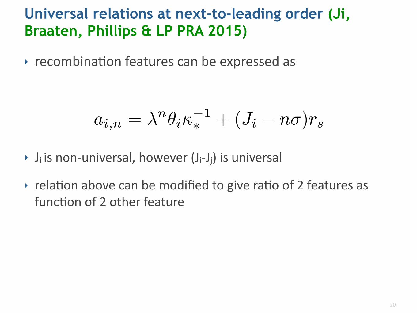
Preliminary: E�ective range correction
• The NLO contribution is an e⇥ective range correction.
• Enters as a tree-level diagram
i�0NLO = i⇥e(Zcore + 1) .
• Charge radius to NLO:
⇥rLO+NLOC ⇤2 = ⇥rLOC ⇤2
�1� 3kCr0 +O(�2/k2
C)⇥�1
• We need experimental or calculated scattering parameters.
E. Ryberg
+
rC,NLO = (2.20± 0.04 (EFT)± 0.11 (ANC)) fm
Determine ANCs from EFT
‣ fitANC(Z-factor)to experimentaldata
‣ obtainANCswitherror esDmatefordifferentorders
10
0 500 1000 1500 2000
E (keV)
2
4
6
8
10
S-fa
ctor
(keV
b)
HEFT N3LOHEFT N5LOMorlock
S-factor value is stable. From these fits we extract a treshold S-factor
S =
⇢ �9.9± 0.1 (fit)± 1.0 (norm.)
�keV b , N3LO�
10.4± 0.1 (fit)± 1.0 (norm.)�keV b , N5LO
(71)
with the 1% error due to the EFT fit (mainly statistical error) and the 10%error from the uncertainty in the absolute normalization of the experimentaldata. These results give the ANC [CF: updated numbers needed.]
A =
⇢ �76.9± 4.3 (fit)± 7.7 (norm.)
�fm�1/2 , N3LO�
78.9± 4.8 (fit)± 7.9 (norm.)�fm�1/2 , N5LO
, (72)
which is consistent with the ANCs of Huang et al and Gagliardi et al .The charge radius of the 17F⇤ can now be obtained by using an extracted
ANC. Using the 16O-proton ANC extracted from the N5LO radiative protoncapture fit, the resulting NLO charge radius is given by [CF: updated numbersneeded.]
rC,NLO = 2.2 fm . (73)
At N2LO the contributions from the proton and 16O charge radii enter. Theresult is [CF: updated numbers needed.]
rC,N2LO =
rr2C,NLO +
1
Zc
r2p +Zc
Zc + 1r216O
=3.4 fm , (74)
using rp = 0.88 fm and r16O = 2.71 fm. [ER: What values should we reallyuse here?]
Since the Coulomb momentum is much larger than the binding momen-tum, it is not clear that the operator d†r2A0d is suppressed to higher order.Therefore one might suspect that the EFT error is substantial for the chargeradius.
7. Conclusions
We have calculated the charge radius and radiative capture cross sectionfor proton halo nuclei interacting through a large S-wave scattering length.Specifically, we have included higher-order e↵ective-range corrections andshown consequent good agreement with experimental data. In particular,our description of proton-capture on 16O agrees very well with the data and
24
compares well with Huang et al. and Gagliardi et al.