Rao-Blackwellised Particle Filtering

Based on Rao-Blackwellised Particle Filtering for Dynamic Bayesian Networks by Arnaud Doucet, Nando de Freitas, Kevin Murphy, and Stuart Russel

Other sources

Artificial Intelligence: A Modern Approach by Stuart Russel and Peter Norvig

Presented by Boris Lipchin

Introduction

PF applications (localization, SLAM, etc) Draw-backs/BenefitsBayes NetsDynamic Bayes NetsParticle FilteringRao-Blackwell PF

Bayes Net Example

Adapted from Artificial Intelligence: A Modern Approach (Norvig and Russell)

What is the probability of Burgalry given that John calls but mary doesn't call?

Bayesian Network

Digraph where edges represent conditional probabilitiesIf A is the parent of B, B is said to be conditioned on AMore compact representation than writing down full joint distribution tablePeople rarely know absolute probability, but can predict conditional probabilities with great accuracy (i.e. doctors and symptoms)

Bayes Net Example

Adapted from Artificial Intelligence: A Modern Approach (Norvig and Russell)

What is the probability of Burgalry given that John calls but mary doesn't call?

Dynamic Bayesian Networks

Represent progress of a system over time1st Order Markov DBN: state variables can only depend on current and previous stateDBNs represent temporal probability distributionsKalman Filter is a special case of a DBNCan model non-linearities (Kalman produces single multivariate Guassian) Untractable to analyze

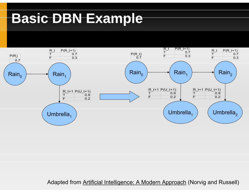
Basic DBN Example

Adapted from Artificial Intelligence: A Modern Approach (Norvig and Russell)

Rain0 Rain1

Umbrella1

0.7P(R

t)

R_t P(R_t+1)T 0.7F 0.3

R_t+1 P(U_t+1)T 0.9F 0.2

Rain0 Rain1

Umbrella1

P(R_t)0.7

R_t P(R_t+1)T 0.7F 0.3

R_t+1 P(U_t+1)T 0.9F 0.2

Rain2

Umbrella2

R_t+1 P(U_t+1)T 0.9F 0.2

R_t P(R_t+1)T 0.7F 0.3

DBN Analysis

Unrolling makes DBNs just like Bayesian NetworkOnline filtering algorithm: variable eliminationAs state grows, complexity of analysis per slice becomes exponential: O( dn+1 ) Necessity for approximate inference

Particle Filtering

Particle Filtering

Constant sample count per slice achieves constant processing timeSamples represent state distributionBut evidence variable (umbrella) never conditions future state (rain)!Weigh future population by evidence likelihoodApplications: localization, SLAM

Particle Filtering: Basic Algorithm

Create initial population:Based on P( X0 )

Update phase: propogate samplesTransition model: P( xt+1 | xt )

Weigh distribution with evidence likelihoodW( xt+1 | e1:t+1 ) = P( et+1 | xt+1 ) * N( xt+1 | e1:t )

Resample to re-create unweighted population of N samples based on created weighted distribution

Visual example

Adapted from Artificial Intelligence: A Modern Approach (Norvig and Russell)

oooooooo

oo

oooooo

oooo

True

False

Raint Raint+1

Propogate

oooooo

oooo

Raint+1

oo

oooooooo

Raint+1

Weight Resample

⌐umbrella

This method converges assymptotically to the real distribution as N → ∞

RBPF

Key concept: decrease number of particles neccessary to achieve same accuracy with regular PFRequirement: Partition state nodes Z(t) into R(t) and X(t) s.t.:

P( R1:t | Y1:t ) can be predicted with PFP( Xt | R1:t,Y1:t ) can be updated analytically/filtered

Paper does not describe partitioning methods, efficient partitioning algorithms are assumed

RBPF: Concept Proof

PF approximates P( Z1:t | Y1:t ) = P( R1:t , X1:t | Y1:t )

Remember state space Z partitioned into R and XP( R1:t , X1:t | Y1:t ) = P( R1:t | Y1:t ) * P( Xt | R1:t,Y1:t )

By chain rule property of probabilitySampling just R requires fewer particles, decreasing complexitySampling X becomes amortized constant time

RBPF DBNs – remember arrows

Adapted from Rao-Blackwellised Particle Filtering for Dynamic Bayesian Networks (Murphy and Russell 2001)

RBPF DBNs

R(t) is called a root, and X(t) a leaf of the DBN(a) Is a canonical DBN to which RBPF can be applied(b) R(t) is a more common partitioning as it simplifies the Particle Filtering of the root in the RBPF(c) Is a convenient partitioning when some root nodes model discontinuous state changes, and others some are the parent of the observation, and model observed outliers

RBPF: Algorithm

Root marginal distribution:δ is the Dirac delta functionw is the weight of the i-th particle at slice t and is computed by

and then normalized.Leaf marginal:

RBPF: Update, Propogate, Weigh

The root particles in RBPF are propogated much like PF particlesThe leaf marginal propogation is computed with an optimal filter (Rao-Blackwellisation step) The leaf and root nodes together compose the entire state of the system, and thus can be weighted and resampled for the next slice.

Example: Localization

SLAM: P( x, m | z, u )= p( m | x, z, u)p( x | z, u )

m is the leaf, x is the root in the RBPFParticle updates based on input, expensive, we keep number of particles down

pose map observations odometryMapping conditioned on position and world

Particle filter for position hypothesis

The Scenario

Assume a world of two blue and yellow states labeled a and b (left to right) A robot can successfuly move between adjacent states with a probabilty Pm=.5 (transition model) The robot is equipped with a color sensor that correctly identifies color with probability Pc=.6

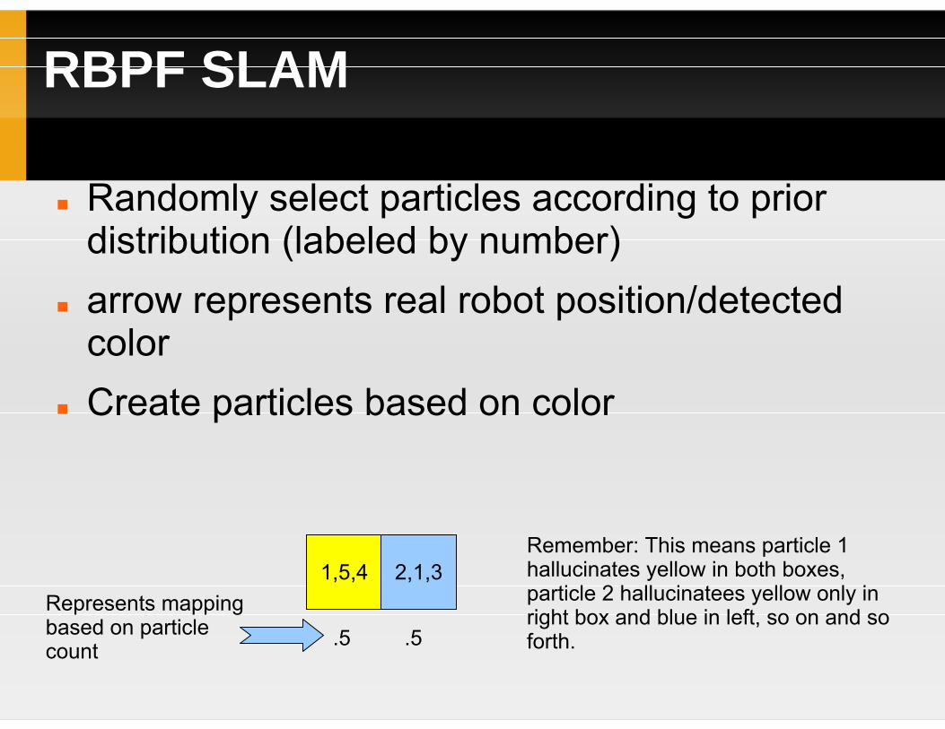
RBPF SLAM

Using N = 5 particlesP(X) represents state distribution (localization) P(M) represents color distribution (mapping) Prior for colors is an even distribution (unmapped) For simplicity, P(X=a) = 1, P(X=b) = 0

RBPF SLAM

Randomly select particles according to prior distribution (labeled by number) arrow represents real robot position/detected colorCreate particles based on color

1,5,4 2,1,3

.5 .5

Remember: This means particle 1 hallucinates yellow in both boxes, particle 2 hallucinatees yellow only in right box and blue in left, so on and so forth.

Represents mapping based on particle count

RBPF SLAM

P(X(t)=a) = 1Calculate weights:

W1 -> P(E(a)=y | M(a)=y,M(b)=y)=P(E(a)=y)*P(M(a)=y | E(a)=y)*P(M(b)=y | E(a)=y,M(a)=y)/

( P(M(a)=y)*P(M(b)=y | M(a)=y) ) =.5 * .6 * .5 / (.5 * .5) = .6

W2 -> P( E(a)=y | M(a)=b,M(b)=y)=P(E(a)=y)*P(M(a)=b | E(a)=y)*P(M(b)=y | E(a)=y, M(a)=b)/

( P(M(a)=b)*P(M(b)=y | M(a)=b) )=.5 * .4 * .5 / (.5 * .5) = .4

You can calculate these guys ad nauseum

1,5,4 2,1,3

robot

.5 .5

RBPF SLAM

P(X(t)=a) = 1Next step is to resample based on weights (shown below) Find P(X(t)) distribution given previous state and current map

1,5,2,4 1,3

robot

.8 .4

RBPF SLAM

Calculate new weightsWeigh samples and resample to obtain updated distribution for the particlesestimate X(t) using optimal filter, evidence, and previous location

1,5,2,4 1,3

robot

.8 .4

RBPF SLAM: Key Ideas

Imagine if X(t) was part of state spaceCalculations increase with number of statesNumber of particles

RBPF simplifies calculations by giving one a ”free” localization with an optimal filter

Questions?