50
Numerical methods for collisional kinetic equations, june 11-18 2003, Wien Part III: Monte Carlo methods Lorenzo Pareschi Department of Mathematics University of Ferrara, Italy 1
Numerical methods for collisional kinetic equations, june 11-18 2003, Wien
Part III: Monte Carlo methods
Lorenzo Pareschi
Department of Mathematics
University of Ferrara, Italy
1
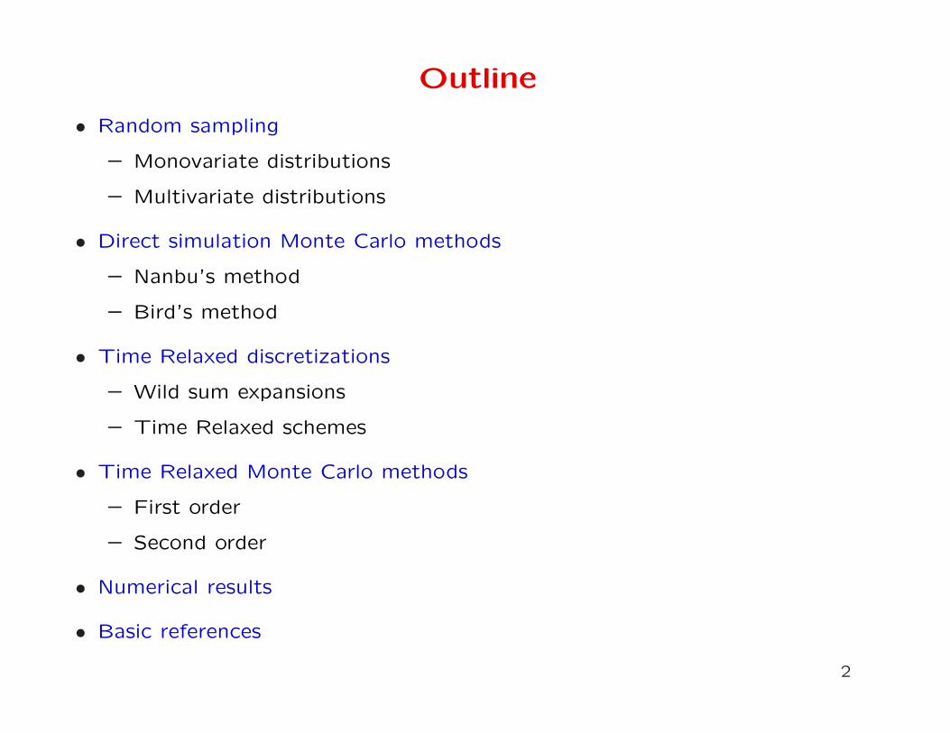
Outline
• Random sampling
– Monovariate distributions
– Multivariate distributions
• Direct simulation Monte Carlo methods
– Nanbu’s method
– Bird’s method
• Time Relaxed discretizations
– Wild sum expansions
– Time Relaxed schemes
• Time Relaxed Monte Carlo methods
– First order
– Second order
• Numerical results
• Basic references
2
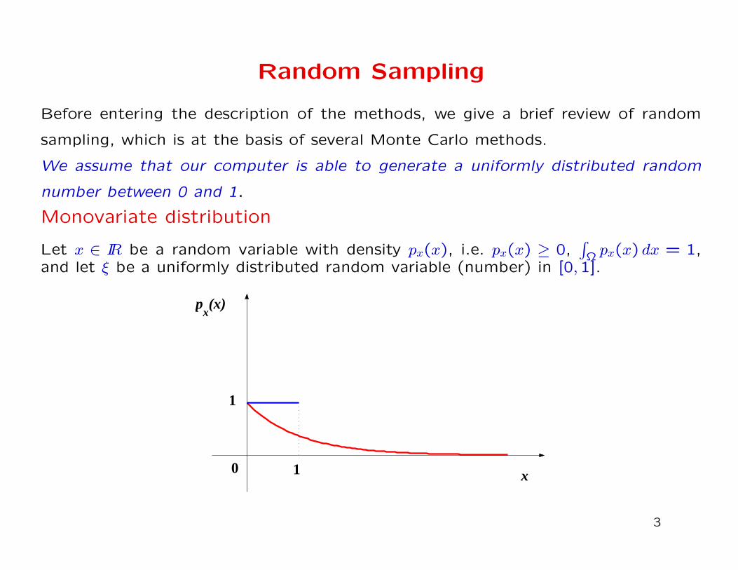
Random Sampling
Before entering the description of the methods, we give a brief review of random
sampling, which is at the basis of several Monte Carlo methods.
We assume that our computer is able to generate a uniformly distributed random
number between 0 and 1.
Monovariate distribution
Let x ∈ IR be a random variable with density px(x), i.e. px(x) ≥ 0,∫Ω px(x) dx = 1,
and let ξ be a uniformly distributed random variable (number) in [0,1].
x
px(x)
1
1 0
3
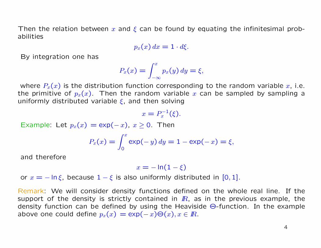
Then the relation between x and ξ can be found by equating the infinitesimal prob-abilities
px(x) dx = 1 · dξ.
By integration one has
Px(x) =
∫ x
−∞px(y) dy = ξ,
where Px(x) is the distribution function corresponding to the random variable x, i.e.the primitive of px(x). Then the random variable x can be sampled by sampling auniformly distributed variable ξ, and then solving
x = P−1x (ξ).
Example: Let px(x) = exp(−x), x ≥ 0. Then
Px(x) =
∫ x
0exp(− y) dy = 1− exp(−x) = ξ,
and therefore
x = − ln(1− ξ)
or x = − ln ξ, because 1− ξ is also uniformly distributed in [0,1].
Remark: We will consider density functions defined on the whole real line. If thesupport of the density is strictly contained in IR, as in the previous example, thedensity function can be defined by using the Heaviside Θ-function. In the exampleabove one could define px(x) = exp(−x)Θ(x), x ∈ IR.
4
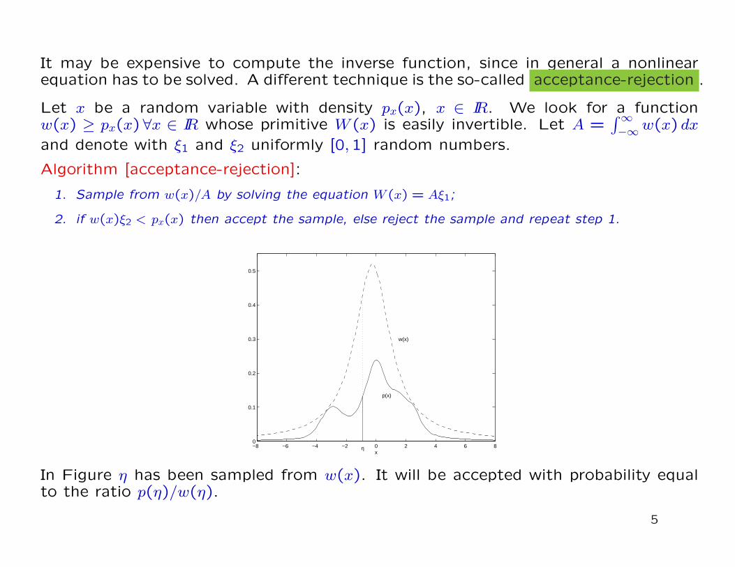
It may be expensive to compute the inverse function, since in general a nonlinearequation has to be solved. A different technique is the so-called acceptance-rejection .
Let x be a random variable with density px(x), x ∈ IR. We look for a functionw(x) ≥ px(x) ∀x ∈ IR whose primitive W (x) is easily invertible. Let A =
∫∞−∞w(x) dx
and denote with ξ1 and ξ2 uniformly [0,1] random numbers.
Algorithm [acceptance-rejection]:
1. Sample from w(x)/A by solving the equation W (x) = Aξ1;
2. if w(x)ξ2 < px(x) then accept the sample, else reject the sample and repeat step 1.
−8 −6 −4 −2 0 2 4 6 80
0.1
0.2
0.3
0.4
0.5
x
p(x)
w(x)
η
In Figure η has been sampled from w(x). It will be accepted with probability equalto the ratio p(η)/w(η).
5
Remark: The efficiency of the scheme depends on how easy it is to invert the functionW (x) and how frequently we accept the sample. The fraction of accepted samplesequals the ratio of the areas below the two curves px(x) and W (x) and it is thereforeequal to 1/A.
Sometimes a density function is given as a convex combination of simpler densityfunctions,
p(x) =M∑
i=1
wipi(x)
where wi are probabilities (i.e. wi ≥ 0,∑M
i=1 wi = 1), and pi(x) are probabilitydensities. In that case the sampling can be performed as follows
Algorithm:
1. select an integer i ∈ 1, . . . , M with probability wi;
2. sample x from a random variable with density pi(x).
Because of the relevance in several applications, step 1 of the previous algorithmdeserves an extended discussion.
6
Discrete sampling
Let us suppose that k ∈ 1, . . . , M is an integer random number, with probabilitieswk. In order to sample k with probability wk we can proceed as follows. Divideinterval [0,1] in M intervals, i-th interval being of length wi, extract a uniform [0,1]random number ξ, and detect the interval k to which ξ belongs in the following way.
Algorithm [discrete sampling 1]:
1. Compute Wk =∑k
i=1wk, k = 1, . . . , M, W0 = 0;
2. find the integer k such that Wk−1 ≤ ξ < Wk.
For an arbitrary set of probabilities wi, once Wi have been computed, step 2 canbe performed with a binary search, in O(lnM) operations.
This approach is efficient if the numbers Wk can be computed once, and then usedseveral times, and if M is not too large. If the number M is very large and the numberswk may change a more efficient acceptance-rejection technique can be used, if atleast an estimate w such that w ≥ wi, i = 1, . . . , M is known.
Algorithm [discrete sampling 2]:
1. Select an integer random number uniformly in [1, . . . , M ], as
k = [[Mξ1]] + 1
where [[x]] denotes the integer part of x;
2. if wkξ2 < w then accept the sampling else reject it and repeat point 1.
7
Clearly the procedure can be generalized to the case in which the estimate dependson k, i.e. wk ≥ wk, k = 1, . . . , M .
The above technique is of crucial relevance in the Monte Carlo simulation of thescattering in the Boltzmann equation.
Sampling without repetition
Sometimes it is useful to extract n numbers, n ≤ N , from the sequence 1, . . . , Nwithout repetition. This sampling is often used in several Monte Carlo simulations.A simple and efficient method to perform the sampling is the following.
Algorithm:
1. set indi = i, i = 1, . . . , N ;
2. M = N ;
3. for i = 1 to n
• set j = [[Mξ]] + 1, seqi = indj,
• indj = indM , M = M − 1
end for
At the end the vector seq will contain n distinct integers randomly sampled fromthe first N natural numbers. Of course if n = N , the vector seq contains a randompermutation of the sequence 1, . . . , N .
8
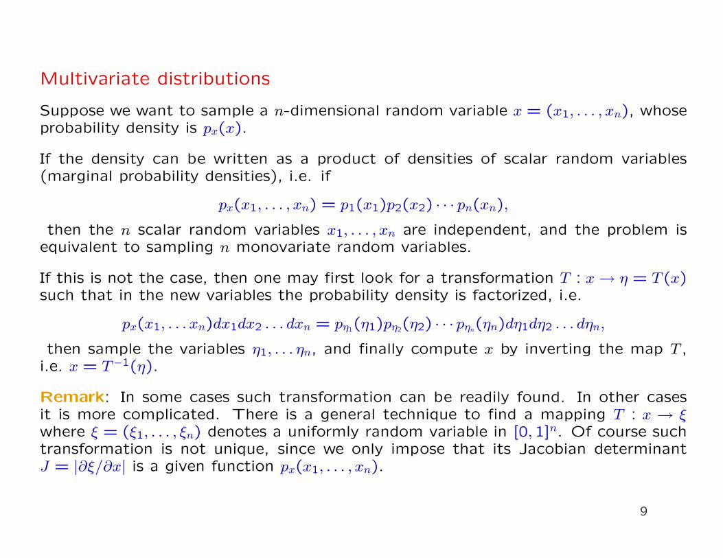
Multivariate distributions
Suppose we want to sample a n-dimensional random variable x = (x1, . . . , xn), whoseprobability density is px(x).
If the density can be written as a product of densities of scalar random variables(marginal probability densities), i.e. if
px(x1, . . . , xn) = p1(x1)p2(x2) · · · pn(xn),
then the n scalar random variables x1, . . . , xn are independent, and the problem isequivalent to sampling n monovariate random variables.
If this is not the case, then one may first look for a transformation T : x → η = T (x)such that in the new variables the probability density is factorized, i.e.
px(x1, . . . xn)dx1dx2 . . . dxn = pη1(η1)pη2(η2) · · · pηn(ηn)dη1dη2 . . . dηn,
then sample the variables η1, . . . ηn, and finally compute x by inverting the map T ,i.e. x = T−1(η).
Remark: In some cases such transformation can be readily found. In other casesit is more complicated. There is a general technique to find a mapping T : x → ξwhere ξ = (ξ1, . . . , ξn) denotes a uniformly random variable in [0,1]n. Of course suchtransformation is not unique, since we only impose that its Jacobian determinantJ = |∂ξ/∂x| is a given function px(x1, . . . , xn).
9
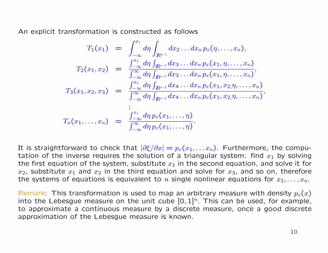
An explicit transformation is constructed as follows
T1(x1) =
∫ x1
−∞dη
∫
IRn−1
dx2 . . . dxn px(η, . . . , xn),
T2(x1, x2) =
∫ x2
−∞ dη∫
IRn−2 dx3 . . . dxn px(x1, η, . . . , xn)∫∞−∞ dη
∫IRn−2 dx3 . . . dxn px(x1, η, . . . , xn)
,
T3(x1, x2, x3) =
∫ x3
−∞ dη∫
IRn−3 dx4 . . . dxn px(x1, x2,η, . . . , xn)∫∞−∞ dη
∫IRn−3 dx4 . . . dxn px(x1, x2,η, . . . , xn)
,
...
Tn(x1, . . . , xn) =
∫ xn
−∞ dη px(x1, . . . , η)∫∞−∞ dη px(x1, . . . , η)
.
It is straightforward to check that |∂ξ/∂x| = px(x1, . . . xn). Furthermore, the compu-tation of the inverse requires the solution of a triangular system: find x1 by solvingthe first equation of the system, substitute x1 in the second equation, and solve it forx2, substitute x1 and x2 in the third equation and solve for x3, and so on, thereforethe systems of equations is equivalent to n single nonlinear equations for x1, . . . , xn.
Remark: This transformation is used to map an arbitrary measure with density px(x)into the Lebesgue measure on the unit cube [0,1]n. This can be used, for example,to approximate a continuous measure by a discrete measure, once a good discreteapproximation of the Lebesgue measure is known.
10
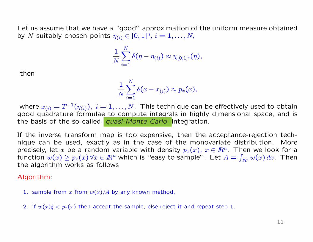
Let us assume that we have a “good” approximation of the uniform measure obtainedby N suitably chosen points η(i) ∈ [0,1]n, i = 1, . . . , N,
1
N
N∑
i=1
δ(η − η(i)) ≈ χ[0,1]n(η),
then
1
N
N∑
i=1
δ(x− x(i)) ≈ px(x),
where x(i) = T−1(η(i)), i = 1, . . . , N . This technique can be effectively used to obtaingood quadrature formulae to compute integrals in highly dimensional space, and isthe basis of the so called quasi-Monte Carlo integration.
If the inverse transform map is too expensive, then the acceptance-rejection tech-nique can be used, exactly as in the case of the monovariate distribution. Moreprecisely, let x be a random variable with density px(x), x ∈ IRn. Then we look for afunction w(x) ≥ px(x) ∀x ∈ IRn which is “easy to sample”. Let A =
∫IRn w(x) dx. Then
the algorithm works as follows
Algorithm:
1. sample from x from w(x)/A by any known method,
2. if w(x)ξ < px(x) then accept the sample, else reject it and repeat step 1.
11
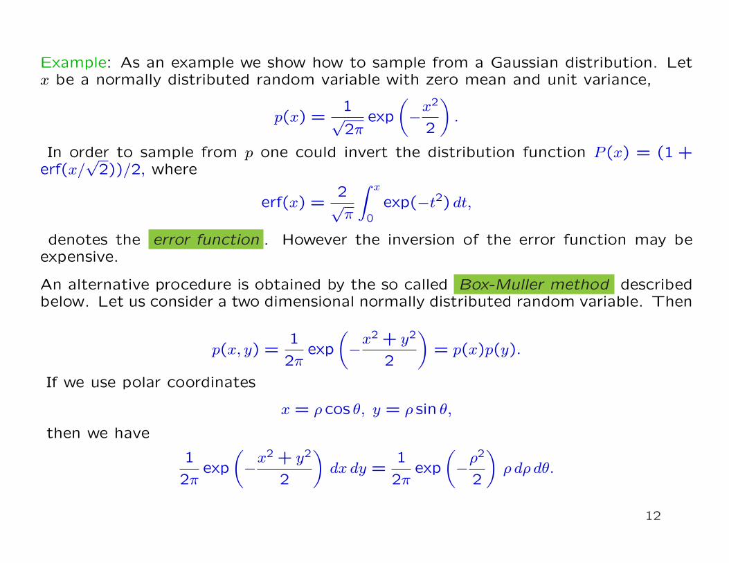
Example: As an example we show how to sample from a Gaussian distribution. Letx be a normally distributed random variable with zero mean and unit variance,
p(x) =1√2π
exp
(−x2
2
).
In order to sample from p one could invert the distribution function P (x) = (1 +erf(x/
√2))/2, where
erf(x) =2√π
∫ x
0exp(−t2) dt,
denotes the error function . However the inversion of the error function may beexpensive.
An alternative procedure is obtained by the so called Box-Muller method describedbelow. Let us consider a two dimensional normally distributed random variable. Then
p(x, y) =1
2πexp
(−x2 + y2
2
)= p(x)p(y).
If we use polar coordinates
x = ρ cos θ, y = ρ sin θ,
then we have
1
2πexp
(−x2 + y2
2
)dx dy =
1
2πexp
(−ρ2
2
)ρ dρ dθ.
12
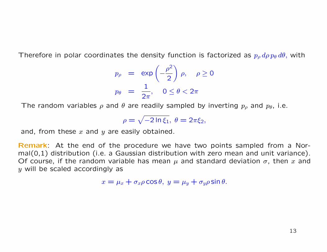
Therefore in polar coordinates the density function is factorized as pρ dρ pθ dθ, with
pρ = exp
(−ρ2
2
)ρ, ρ ≥ 0
pθ =1
2π, 0 ≤ θ < 2π
The random variables ρ and θ are readily sampled by inverting pρ and pθ, i.e.
ρ =√−2 ln ξ1, θ = 2πξ2,
and, from these x and y are easily obtained.
Remark: At the end of the procedure we have two points sampled from a Nor-mal(0,1) distribution (i.e. a Gaussian distribution with zero mean and unit variance).Of course, if the random variable has mean µ and standard deviation σ, then x andy will be scaled accordingly as
x = µx + σxρ cos θ, y = µy + σyρ sin θ.
13
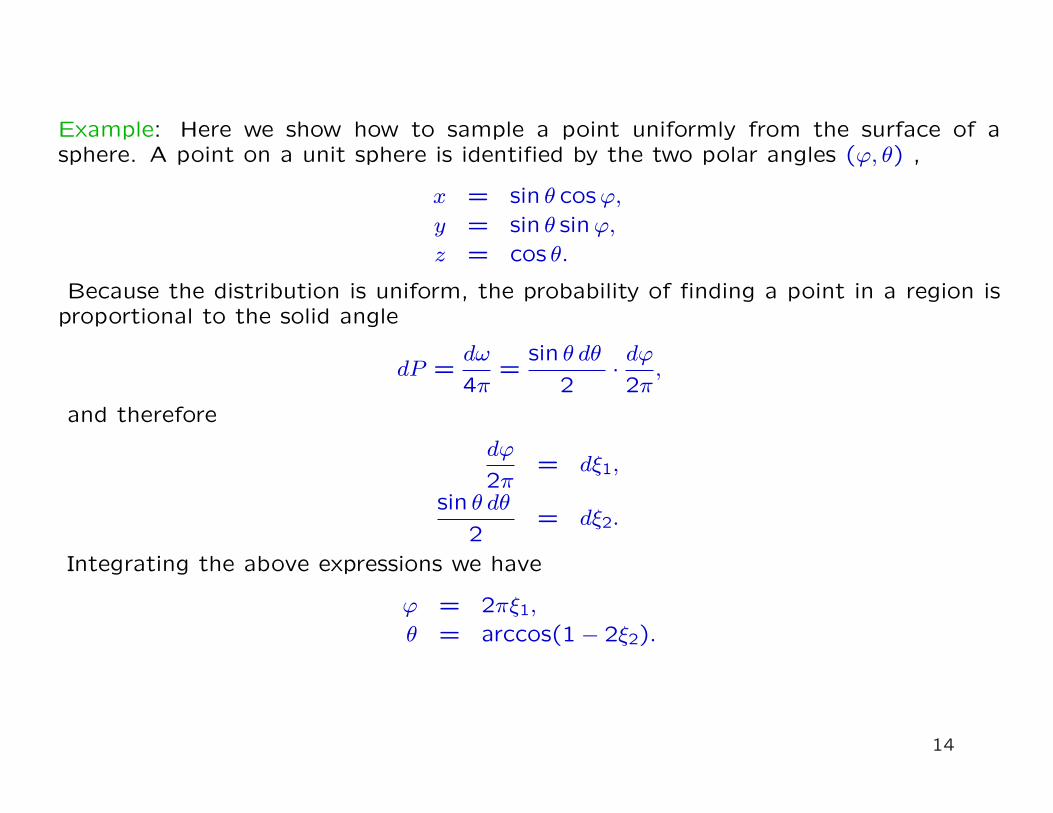
Example: Here we show how to sample a point uniformly from the surface of asphere. A point on a unit sphere is identified by the two polar angles (ϕ, θ) ,
x = sin θ cosϕ,
y = sin θ sinϕ,
z = cos θ.
Because the distribution is uniform, the probability of finding a point in a region isproportional to the solid angle
dP =dω
4π=
sin θ dθ
2· dϕ
2π,
and therefore
dϕ
2π= dξ1,
sin θ dθ
2= dξ2.
Integrating the above expressions we have
ϕ = 2πξ1,
θ = arccos(1− 2ξ2).
14
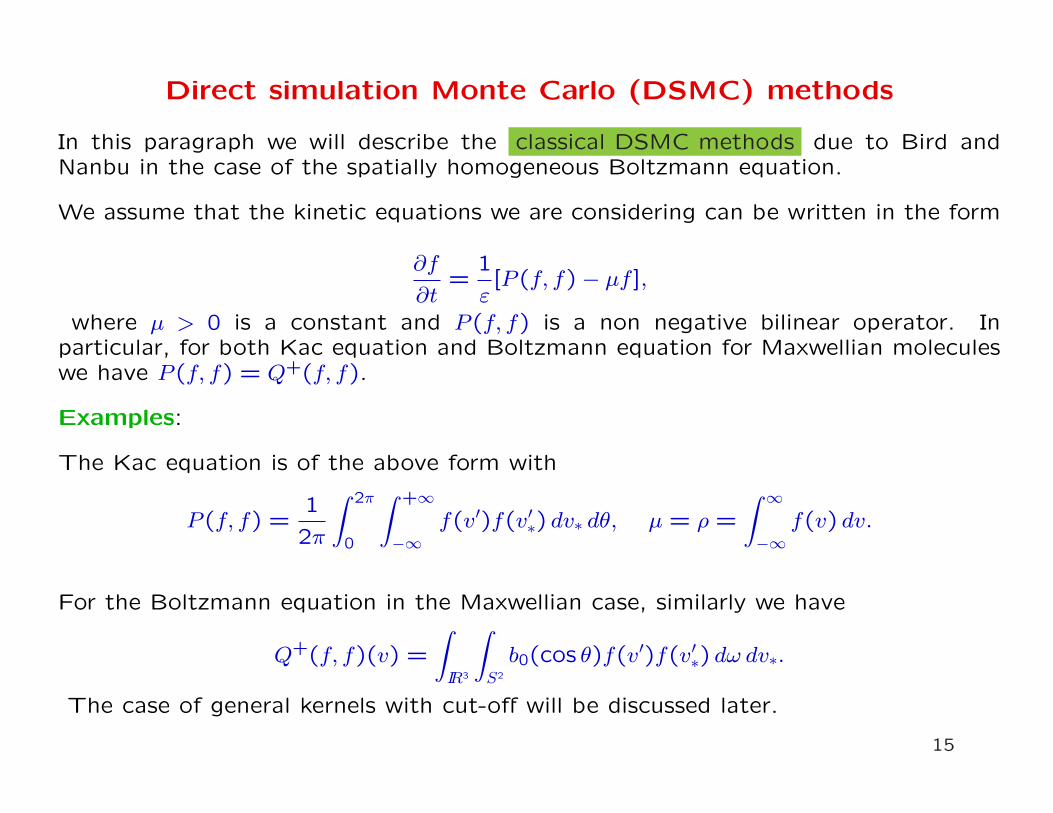
Direct simulation Monte Carlo (DSMC) methods
In this paragraph we will describe the classical DSMC methods due to Bird andNanbu in the case of the spatially homogeneous Boltzmann equation.
We assume that the kinetic equations we are considering can be written in the form
∂f
∂t=
1
ε[P (f, f)− µf ],
where µ > 0 is a constant and P (f, f) is a non negative bilinear operator. Inparticular, for both Kac equation and Boltzmann equation for Maxwellian moleculeswe have P (f, f) = Q+(f, f).
Examples:
The Kac equation is of the above form with
P (f, f) =1
2π
∫ 2π
0
∫ +∞
−∞f(v′)f(v′∗) dv∗ dθ, µ = ρ =
∫ ∞
−∞f(v) dv.
For the Boltzmann equation in the Maxwellian case, similarly we have
Q+(f, f)(v) =
∫
IR3
∫
S2
b0(cos θ)f(v′)f(v′∗) dω dv∗.
The case of general kernels with cut-off will be discussed later.
15
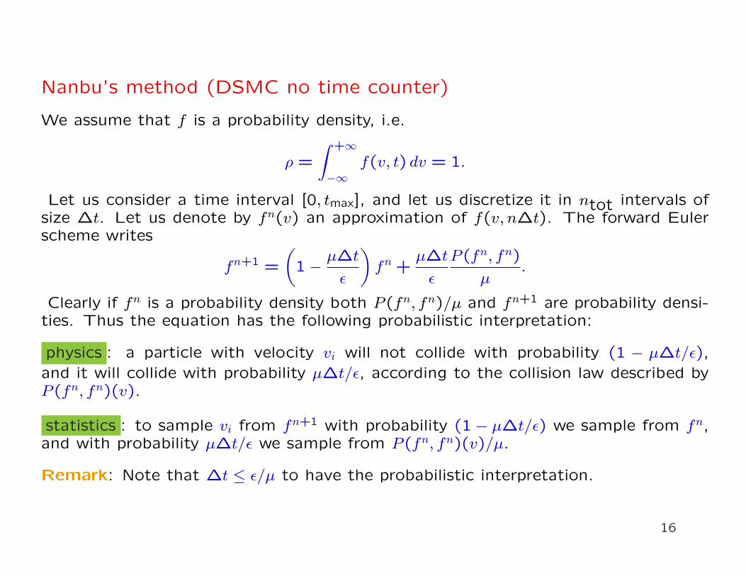
Nanbu’s method (DSMC no time counter)
We assume that f is a probability density, i.e.
ρ =
∫ +∞
−∞f(v, t) dv = 1.
Let us consider a time interval [0, tmax], and let us discretize it in ntot intervals ofsize ∆t. Let us denote by fn(v) an approximation of f(v, n∆t). The forward Eulerscheme writes
fn+1 =
(1− µ∆t
ε
)fn +
µ∆t
ε
P (fn, fn)
µ.
Clearly if fn is a probability density both P (fn, fn)/µ and fn+1 are probability densi-ties. Thus the equation has the following probabilistic interpretation:
physics : a particle with velocity vi will not collide with probability (1 − µ∆t/ε),and it will collide with probability µ∆t/ε, according to the collision law described byP (fn, fn)(v).
statistics : to sample vi from fn+1 with probability (1− µ∆t/ε) we sample from fn,and with probability µ∆t/ε we sample from P (fn, fn)(v)/µ.
Remark: Note that ∆t ≤ ε/µ to have the probabilistic interpretation.
16
Maxwellian case
Let us consider first kinetic equations for which P (f, f) = Q+(f, f), i.e. the collisionkernel does not depend on the relative velocity of the particles.
An algorithm based on this probabilistic interpretation was proposed by Nanbu.
Algorithm[Nanbu for Maxwell molecules]:
1. compute the initial velocity of the particles, v0i , i = 1, . . . , N,
by sampling them from the initial density f0(v)2. for n = 1 to ntot
for i = 1 to Nwith probability 1− µ∆t/ε
set vn+1i = vn
iwith probability µ∆t/ε
select a random particle j compute v′i by performing the collisionbetween particle i and particle j
assign vn+1i = v′i
end forend for
Remark: In its first version, Nanbu’s algorithm was not conservative, i.e. energywas conserved only in the mean, but not at each collision. A conservative versionof the algorithm was introduced by Babovsky. Instead of selecting single particles,independent particle pairs are selected, and conservation is maintained at each col-lision.
17
The expected number of particles that collide in a small time step ∆t is Nµ∆t/ε, andthe expected number of collision pairs is Nµ∆t/(2ε). The algorithm is the following
Algorithm[Nanbu-Babovsky for Maxwell molecules]:
1. compute the initial velocity of the particles, v0i , i = 1, . . . , N,
by sampling them from the initial density f0(v)2. for n = 1 to ntot
given vni , i = 1, . . . , N
set Nc = Iround(µN∆t/(2ε) select Nc pairs (i, j) uniformly among all possible pairs,and for those- perform the collision between i and j, and compute
v′i and v′j according to the collision law
- set vn+1i = v′i, vn+1
j = v′j set vn+1
i = vni for all the particles that have not been selected
end for
Here by Iround(x) we denote a suitable integer rounding of a positive real numberx. For example
Iround(x) =
[[x]] + 1 with probability x− [[x]][[x]] with probability [[x]] + 1− x
where [[x]] denotes the integer part of x.
Remark: As we said before, the algorithm just described can be applied to the Kacequation and to the homogeneous Boltzmann equation with Maxwellian molecules.The only difference in the two cases consists in the computation of the post-collisionalvelocities.
18
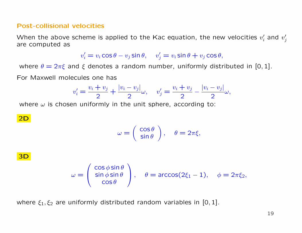
Post-collisional velocities
When the above scheme is applied to the Kac equation, the new velocities v′i and v′jare computed as
v′i = vi cos θ − vj sin θ, v′j = vi sin θ + vj cos θ,
where θ = 2πξ and ξ denotes a random number, uniformly distributed in [0,1].
For Maxwell molecules one has
v′i =vi + vj
2+|vi − vj|
2ω, v′j =
vi + vj
2− |vi − vj|
2ω,
where ω is chosen uniformly in the unit sphere, according to:
2D
ω =
(cos θsin θ
), θ = 2πξ,
3D
ω =
cosφ sin θsinφ sin θ
cos θ
, θ = arccos(2ξ1 − 1), φ = 2πξ2,
where ξ1, ξ2 are uniformly distributed random variables in [0,1].
19
Variable Hard Sphere case
The above algorithm has to be modified when the scattering cross section is notconstant. To this aim we shall assume that the collision kernel satisfies some cut-offhypothesis, which is essential from a numerical point of view.
We will denote by QΣ(f, f) the collision operator obtained by replacing the kernel Bwith the kernel BΣ
BΣ(|v − v∗|) = min B(|v − v∗|),Σ , Σ > 0.
Thus, for a fixed Σ, let us consider the homogeneous problem
∂f
∂t=
1
εQΣ(f, f).
The operator QΣ(f, f) can be written in the form P (f, f)− µf taking
P (f, f) = Q+Σ(f, f) + f(v)
∫
IR3
∫
S2
[Σ−BΣ(|v − v∗|)]f(v∗) dω dv∗,
with µ = 4πΣρ and
Q+Σ(f, f) =
∫
IR3
∫
S2
BΣ(|v − v∗|)f(v′)f(v′∗) dω dv∗.
Remark: In this case, a simple scheme is obtained by using the acceptance-rejectiontechnique to sample the post collisional velocity according to P (f, f)/µ, where µ =4πΣρ and Σ is an upper bound of the scattering cross section.
20
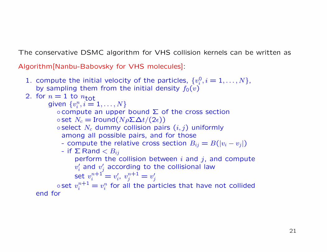
The conservative DSMC algorithm for VHS collision kernels can be written as
Algorithm[Nanbu-Babovsky for VHS molecules]:
1. compute the initial velocity of the particles, v0i , i = 1, . . . , N,
by sampling them from the initial density f0(v)2. for n = 1 to ntot
given vni , i = 1, . . . , N
compute an upper bound Σ of the cross section set Nc = Iround(NρΣ∆t/(2ε)) select Nc dummy collision pairs (i, j) uniformlyamong all possible pairs, and for those- compute the relative cross section Bij = B(|vi − vj|)- if ΣRand < Bij
perform the collision between i and j, and computev′i and v′j according to the collisional law
set vn+1i = v′i, vn+1
j = v′j set vn+1
i = vni for all the particles that have not collided
end for
21
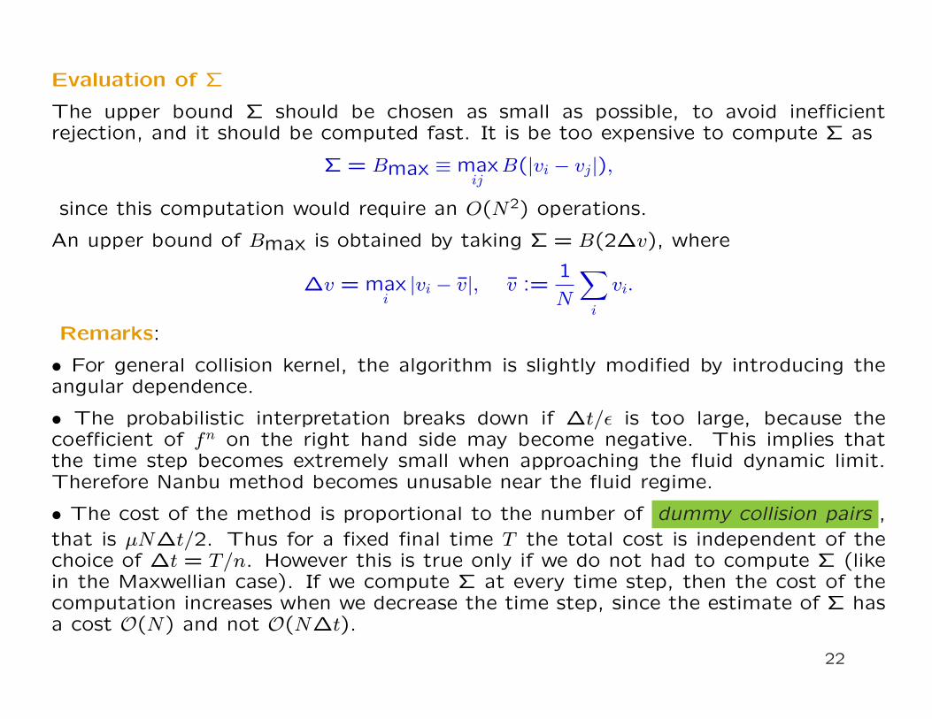
Evaluation of Σ
The upper bound Σ should be chosen as small as possible, to avoid inefficientrejection, and it should be computed fast. It is be too expensive to compute Σ as
Σ = Bmax ≡ maxij
B(|vi − vj|),
since this computation would require an O(N2) operations.
An upper bound of Bmax is obtained by taking Σ = B(2∆v), where
∆v = maxi|vi − v|, v :=
1
N
∑
i
vi.
Remarks:
• For general collision kernel, the algorithm is slightly modified by introducing theangular dependence.
• The probabilistic interpretation breaks down if ∆t/ε is too large, because thecoefficient of fn on the right hand side may become negative. This implies thatthe time step becomes extremely small when approaching the fluid dynamic limit.Therefore Nanbu method becomes unusable near the fluid regime.
• The cost of the method is proportional to the number of dummy collision pairs ,that is µN∆t/2. Thus for a fixed final time T the total cost is independent of thechoice of ∆t = T/n. However this is true only if we do not had to compute Σ (likein the Maxwellian case). If we compute Σ at every time step, then the cost of thecomputation increases when we decrease the time step, since the estimate of Σ hasa cost O(N) and not O(N∆t).
22
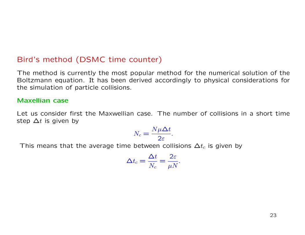
Bird’s method (DSMC time counter)
The method is currently the most popular method for the numerical solution of theBoltzmann equation. It has been derived accordingly to physical considerations forthe simulation of particle collisions.
Maxellian case
Let us consider first the Maxwellian case. The number of collisions in a short timestep ∆t is given by
Nc =Nµ∆t
2ε.
This means that the average time between collisions ∆tc is given by
∆tc =∆t
Nc=
2ε
µN.
23
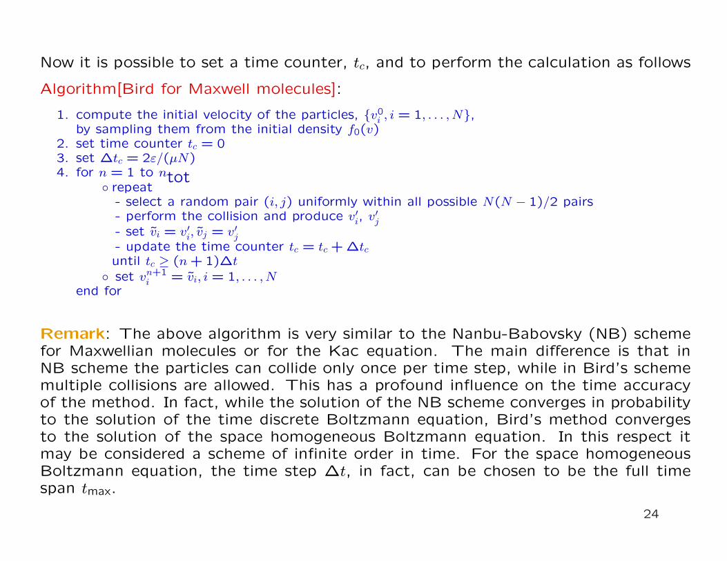
Now it is possible to set a time counter, tc, and to perform the calculation as follows
Algorithm[Bird for Maxwell molecules]:
1. compute the initial velocity of the particles, v0i , i = 1, . . . , N,
by sampling them from the initial density f0(v)2. set time counter tc = 03. set ∆tc = 2ε/(µN)4. for n = 1 to ntot repeat
- select a random pair (i, j) uniformly within all possible N(N − 1)/2 pairs- perform the collision and produce v′i, v′j- set vi = v′i, vj = v′j- update the time counter tc = tc + ∆tcuntil tc ≥ (n + 1)∆t
set vn+1i = vi, i = 1, . . . , N
end for
Remark: The above algorithm is very similar to the Nanbu-Babovsky (NB) schemefor Maxwellian molecules or for the Kac equation. The main difference is that inNB scheme the particles can collide only once per time step, while in Bird’s schememultiple collisions are allowed. This has a profound influence on the time accuracyof the method. In fact, while the solution of the NB scheme converges in probabilityto the solution of the time discrete Boltzmann equation, Bird’s method convergesto the solution of the space homogeneous Boltzmann equation. In this respect itmay be considered a scheme of infinite order in time. For the space homogeneousBoltzmann equation, the time step ∆t, in fact, can be chosen to be the full timespan tmax.
24
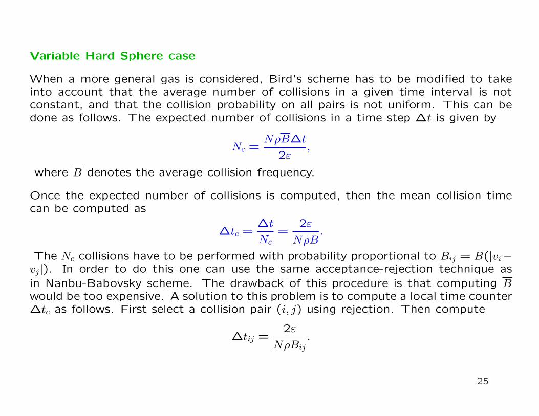
Variable Hard Sphere case
When a more general gas is considered, Bird’s scheme has to be modified to takeinto account that the average number of collisions in a given time interval is notconstant, and that the collision probability on all pairs is not uniform. This can bedone as follows. The expected number of collisions in a time step ∆t is given by
Nc =NρB∆t
2ε,
where B denotes the average collision frequency.
Once the expected number of collisions is computed, then the mean collision timecan be computed as
∆tc =∆t
Nc=
2ε
NρB.
The Nc collisions have to be performed with probability proportional to Bij = B(|vi−vj|). In order to do this one can use the same acceptance-rejection technique asin Nanbu-Babovsky scheme. The drawback of this procedure is that computing Bwould be too expensive. A solution to this problem is to compute a local time counter∆tc as follows. First select a collision pair (i, j) using rejection. Then compute
∆tij =2ε
NρBij.
25
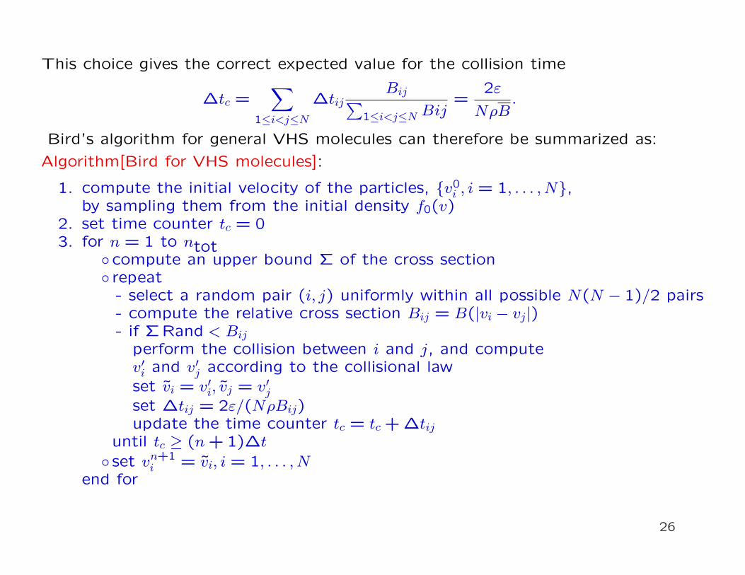
This choice gives the correct expected value for the collision time
∆tc =∑
1≤i<j≤N
∆tijBij∑
1≤i<j≤N Bij=
2ε
NρB.
Bird’s algorithm for general VHS molecules can therefore be summarized as:
Algorithm[Bird for VHS molecules]:
1. compute the initial velocity of the particles, v0i , i = 1, . . . , N,
by sampling them from the initial density f0(v)2. set time counter tc = 03. for n = 1 to ntotcompute an upper bound Σ of the cross section
repeat- select a random pair (i, j) uniformly within all possible N(N − 1)/2 pairs- compute the relative cross section Bij = B(|vi − vj|)- if ΣRand < Bij
perform the collision between i and j, and computev′i and v′j according to the collisional lawset vi = v′i, vj = v′jset ∆tij = 2ε/(NρBij)update the time counter tc = tc + ∆tij
until tc ≥ (n + 1)∆t
set vn+1i = vi, i = 1, . . . , N
end for
26
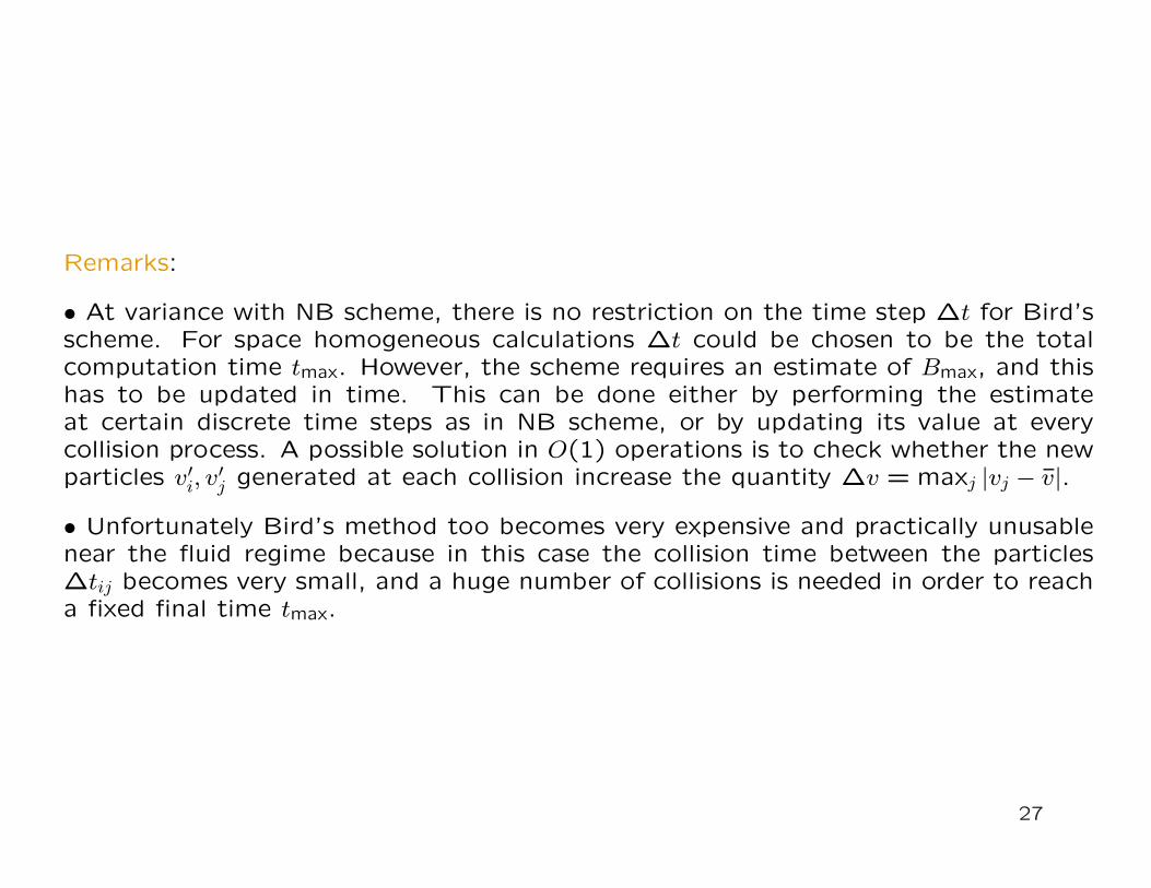
Remarks:
• At variance with NB scheme, there is no restriction on the time step ∆t for Bird’sscheme. For space homogeneous calculations ∆t could be chosen to be the totalcomputation time tmax. However, the scheme requires an estimate of Bmax, and thishas to be updated in time. This can be done either by performing the estimateat certain discrete time steps as in NB scheme, or by updating its value at everycollision process. A possible solution in O(1) operations is to check whether the newparticles v′i, v
′j generated at each collision increase the quantity ∆v = maxj |vj − v|.
• Unfortunately Bird’s method too becomes very expensive and practically unusablenear the fluid regime because in this case the collision time between the particles∆tij becomes very small, and a huge number of collisions is needed in order to reacha fixed final time tmax.
27
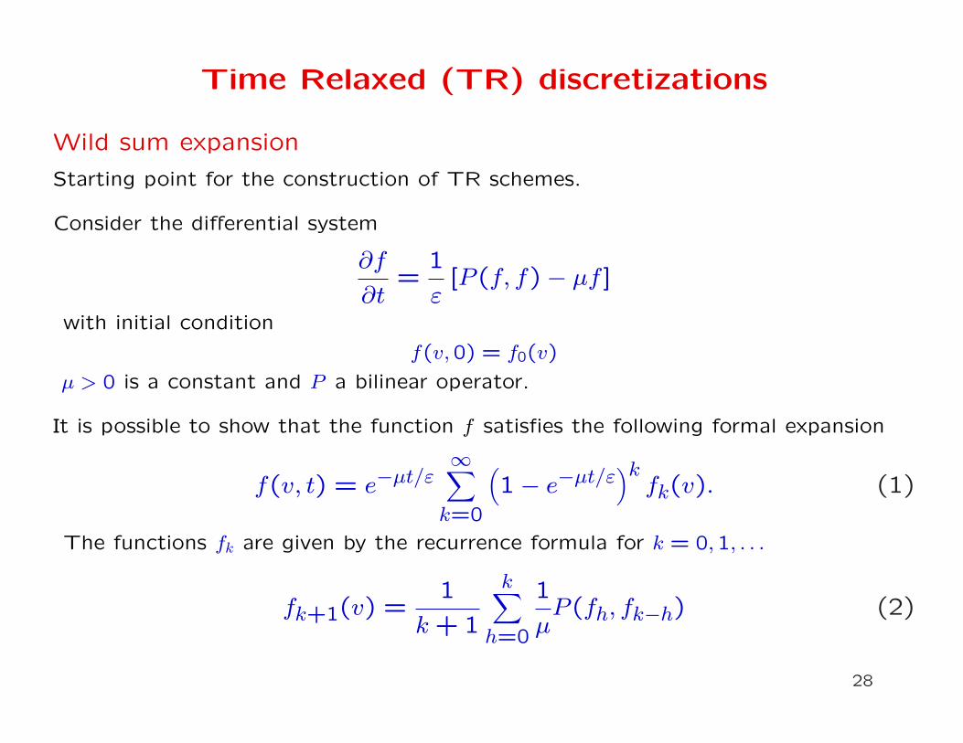
Time Relaxed (TR) discretizations
Wild sum expansion
Starting point for the construction of TR schemes.
Consider the differential system
∂f
∂t=
1
ε[P (f, f)− µf ]
with initial condition
f(v,0) = f0(v)
µ > 0 is a constant and P a bilinear operator.
It is possible to show that the function f satisfies the following formal expansion
f(v, t) = e−µt/ε∞∑
k=0
(1− e−µt/ε
)kfk(v). (1)
The functions fk are given by the recurrence formula for k = 0,1, . . .
fk+1(v) =1
k + 1
k∑
h=0
1
µP (fh, fk−h) (2)
28
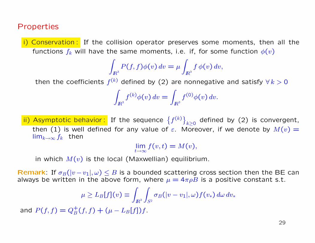
Properties
i) Conservation : If the collision operator preserves some moments, then all the
functions fk will have the same moments, i.e. if, for some function φ(v)∫
IR3
P (f, f)φ(v) dv = µ
∫
IR3
f φ(v) dv,
then the coefficients f (k) defined by (2) are nonnegative and satisfy ∀ k > 0∫
IR3
f (k)φ(v) dv =
∫
IR3
f (0)φ(v) dv.
ii) Asymptotic behavior : If the sequencef (k)
k≥0
defined by (2) is convergent,
then (1) is well defined for any value of ε. Moreover, if we denote by M(v) =limk→∞ fk then
limt→∞
f(v, t) = M(v),
in which M(v) is the local (Maxwellian) equilibrium.
Remark: If σB(|v−v1|, ω) ≤ B is a bounded scattering cross section then the BE canalways be written in the above form, where µ = 4πρB is a positive constant s.t.
µ ≥ LB[f ](v) ≡∫
IR3
∫
S2
σB(|v − v1|, ω)f(v∗) dω dv∗
and P (f, f) = Q+B (f, f) + (µ− LB[f ])f .
29
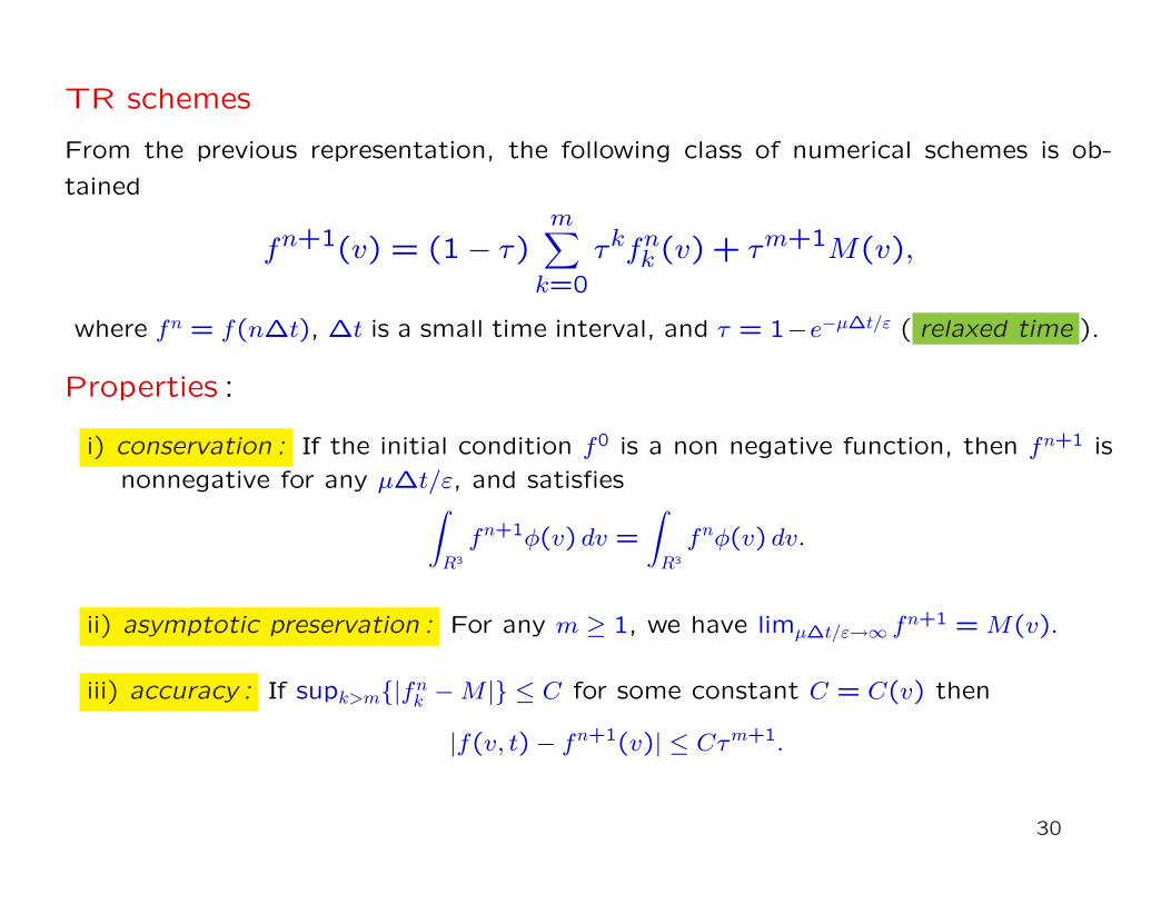
TR schemes
From the previous representation, the following class of numerical schemes is ob-
tained
fn+1(v) = (1− τ)m∑
k=0
τkfnk (v) + τm+1M(v),
where fn = f(n∆t), ∆t is a small time interval, and τ = 1−e−µ∆t/ε ( relaxed time ).
Properties :
i) conservation : If the initial condition f0 is a non negative function, then fn+1 is
nonnegative for any µ∆t/ε, and satisfies∫
R3
fn+1φ(v) dv =
∫
R3
fnφ(v) dv.
ii) asymptotic preservation : For any m ≥ 1, we have limµ∆t/ε→∞ fn+1 = M(v).
iii) accuracy : If supk>m|fnk −M | ≤ C for some constant C = C(v) then
|f(v, t)− fn+1(v)| ≤ Cτm+1.
30
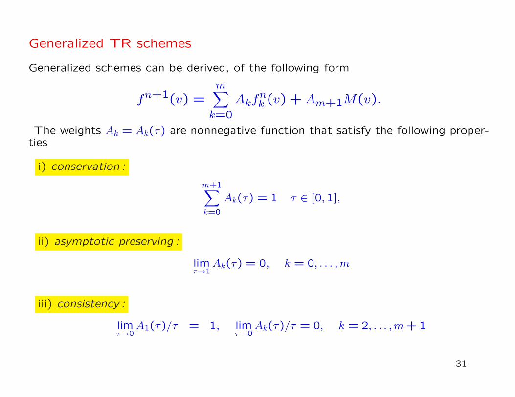
Generalized TR schemes
Generalized schemes can be derived, of the following form
fn+1(v) =m∑
k=0
Akfnk (v) + Am+1M(v).
The weights Ak = Ak(τ) are nonnegative function that satisfy the following proper-ties
i) conservation :
m+1∑
k=0
Ak(τ) = 1 τ ∈ [0,1],
ii) asymptotic preserving :
limτ→1
Ak(τ) = 0, k = 0, . . . , m
iii) consistency :
limτ→0
A1(τ)/τ = 1, limτ→0
Ak(τ)/τ = 0, k = 2, . . . , m + 1
31
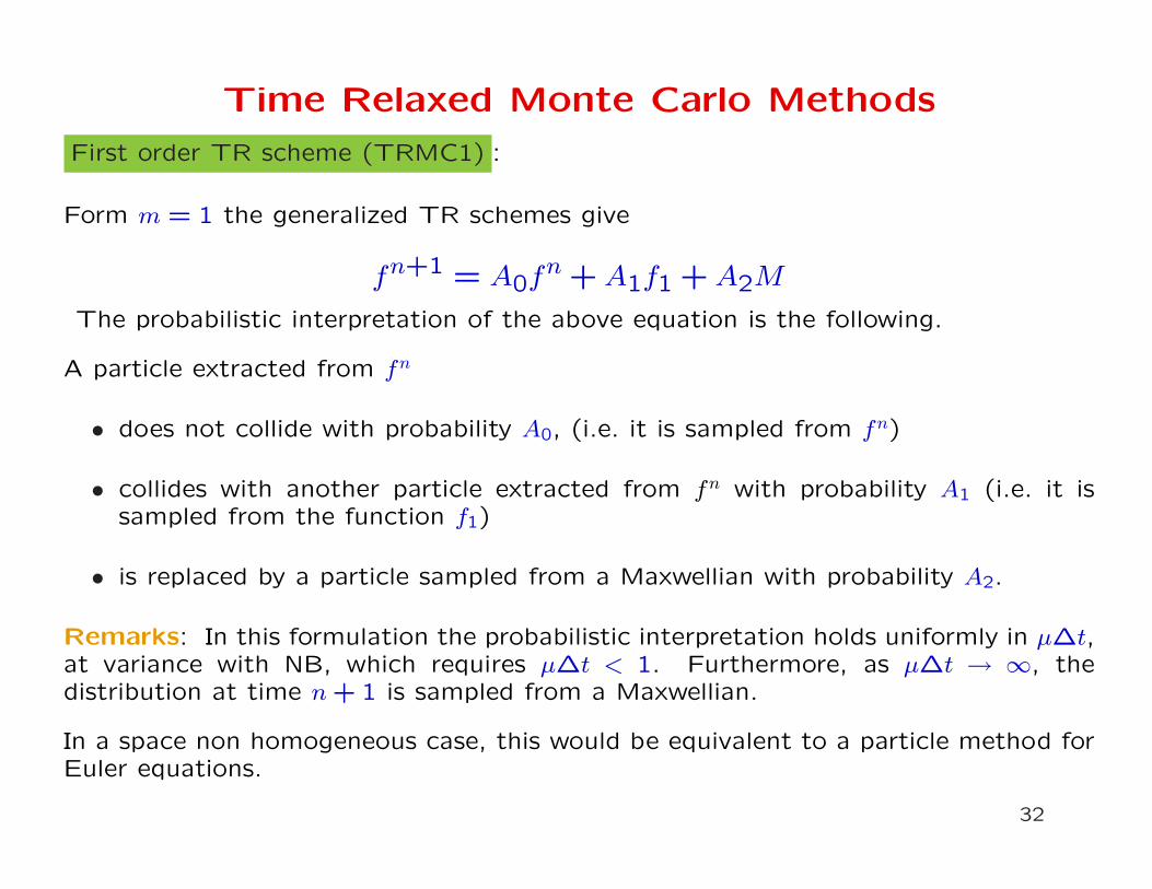
Time Relaxed Monte Carlo Methods
First order TR scheme (TRMC1) :
Form m = 1 the generalized TR schemes give
fn+1 = A0fn + A1f1 + A2M
The probabilistic interpretation of the above equation is the following.
A particle extracted from fn
• does not collide with probability A0, (i.e. it is sampled from fn)
• collides with another particle extracted from fn with probability A1 (i.e. it issampled from the function f1)
• is replaced by a particle sampled from a Maxwellian with probability A2.
Remarks: In this formulation the probabilistic interpretation holds uniformly in µ∆t,at variance with NB, which requires µ∆t < 1. Furthermore, as µ∆t → ∞, thedistribution at time n + 1 is sampled from a Maxwellian.
In a space non homogeneous case, this would be equivalent to a particle method forEuler equations.
32
Second order TR scheme (TRMC2) :
Form m = 2 the generalized TR schemes give
fn+1 = A0fn + A1f1 + A2f2 + A3M,
with f1 = P (fn, fn)/µ, f2 = P (fn, f1)/µ.
The probabilistic interpretation of the scheme is the following. Given N particlesdistributed according to fn:
• NA0 particles do not collide,
• NA1 are sampled from f1, as in the first order scheme,
• NA2 are sampled from f2, i.e. NA2/2 particles sampled from fn will undergodummy collisions with NA2/2 particles sampled from f1,
• NA3 particles are sampled from a Maxwellian.
Remarks: Previous MC schemes can be made exactly conservative. This goal isachieved by using a suitable algorithm for sampling a set of particles with prescribedmomentum and energy from a Maxwellian.
Similarly, higher order TRMC methods can be constructed. For example, a thirdorder scheme is obtained from
fn+1 = A0fn + A1f1 + A2f2 + A3f3 + A4M
with f1 = P (fn, fn)/µ, f2 = P (fn, f1)/µ and f3 = [2P (fn, f2) + P (f1, f1)]/3µ.
33
Numerical results
Space homogeneous case
Comparison between:
NB , TRMC1 , TRMC2 , TRMC3 .
Test problems:
Exact solution for the Kac equation
Exact solution for Maxwell molecules
Remarks The function is reconstructed on a regular grid by convolving the particledistribution with a suitable mollifier.
Number of particles : N = 5× 10⁴ (1d) N = 5× 10⁵ (2d)
34
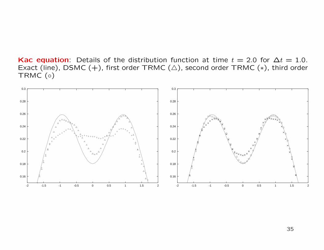
Kac equation: Details of the distribution function at time t = 2.0 for ∆t = 1.0.Exact (line), DSMC (+), first order TRMC (4), second order TRMC (∗), third orderTRMC ()
0.16
0.18
0.2
0.22
0.24
0.26
0.28
0.3
-2 -1.5 -1 -0.5 0 0.5 1 1.5 2
0.16
0.18
0.2
0.22
0.24
0.26
0.28
0.3
-2 -1.5 -1 -0.5 0 0.5 1 1.5 2
35
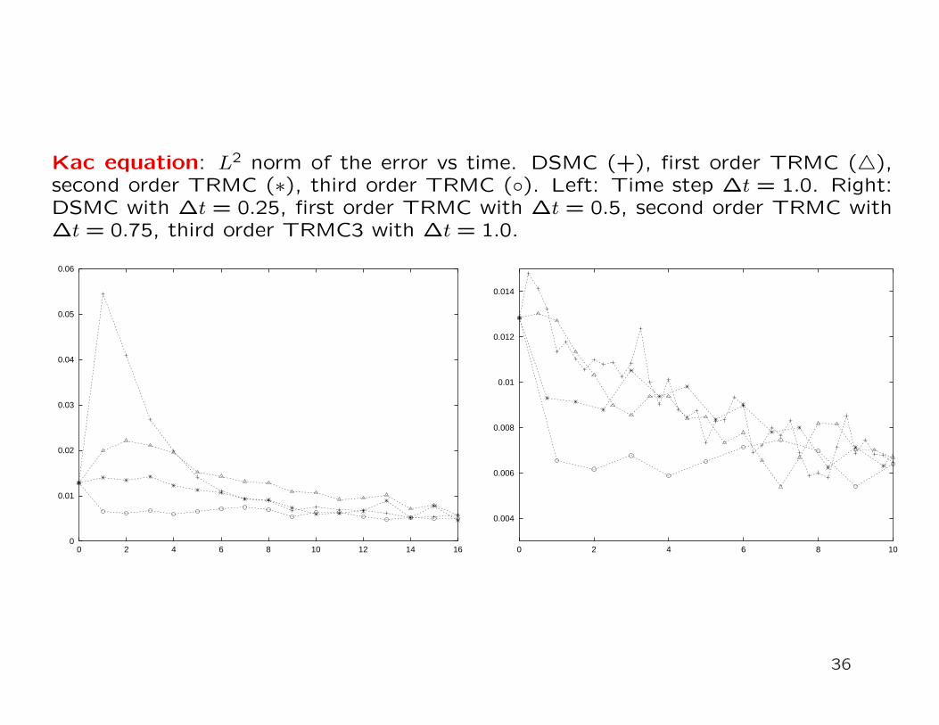
Kac equation: L2 norm of the error vs time. DSMC (+), first order TRMC (4),second order TRMC (∗), third order TRMC (). Left: Time step ∆t = 1.0. Right:DSMC with ∆t = 0.25, first order TRMC with ∆t = 0.5, second order TRMC with∆t = 0.75, third order TRMC3 with ∆t = 1.0.
0
0.01
0.02
0.03
0.04
0.05
0.06
0 2 4 6 8 10 12 14 16
0.004
0.006
0.008
0.01
0.012
0.014
0 2 4 6 8 10
36
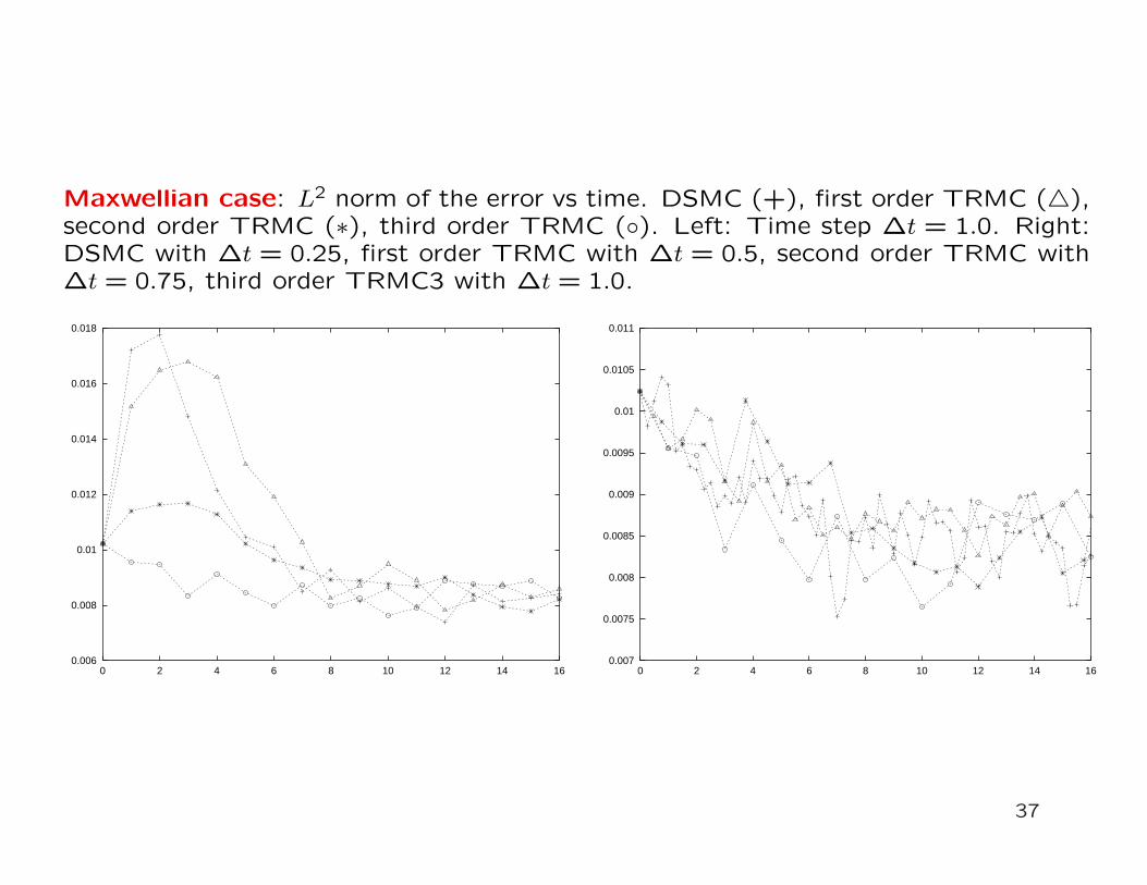
Maxwellian case: L2 norm of the error vs time. DSMC (+), first order TRMC (4),second order TRMC (∗), third order TRMC (). Left: Time step ∆t = 1.0. Right:DSMC with ∆t = 0.25, first order TRMC with ∆t = 0.5, second order TRMC with∆t = 0.75, third order TRMC3 with ∆t = 1.0.
0.006
0.008
0.01
0.012
0.014
0.016
0.018
0 2 4 6 8 10 12 14 160.007
0.0075
0.008
0.0085
0.009
0.0095
0.01
0.0105
0.011
0 2 4 6 8 10 12 14 16
37
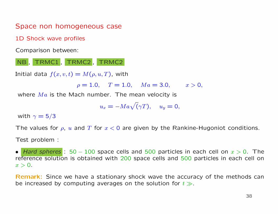
Space non homogeneous case
1D Shock wave profiles
Comparison between:
NB , TRMC1 , TRMC2 , TRMC2
Initial data f(x, v, t) = M(ρ, u, T ), with
ρ = 1.0, T = 1.0, Ma = 3.0, x > 0,
where Ma is the Mach number. The mean velocity is
ux = −Ma√
(γT ), uy = 0,
with γ = 5/3
The values for ρ, u and T for x < 0 are given by the Rankine-Hugoniot conditions.
Test problem :
• Hard spheres : 50 − 100 space cells and 500 particles in each cell on x > 0. Thereference solution is obtained with 200 space cells and 500 particles in each cell onx > 0.
Remark: Since we have a stationary shock wave the accuracy of the methods canbe increased by computing averages on the solution for t À.
38
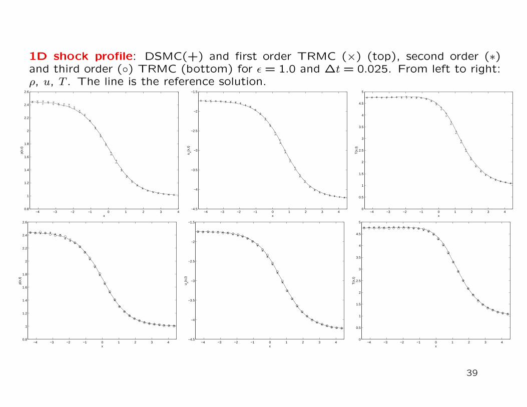
1D shock profile: DSMC(+) and first order TRMC (×) (top), second order (∗)and third order () TRMC (bottom) for ε = 1.0 and ∆t = 0.025. From left to right:ρ, u, T . The line is the reference solution.
−4 −3 −2 −1 0 1 2 3 40.8
1
1.2
1.4
1.6
1.8
2
2.2
2.4
2.6
x
ρ(x,
t)
−4 −3 −2 −1 0 1 2 3 4−4.5
−4
−3.5
−3
−2.5
−2
−1.5
x
u x(x,t)
−4 −3 −2 −1 0 1 2 3 40
0.5
1
1.5
2
2.5
3
3.5
4
4.5
5
x
T(x
,t)
−4 −3 −2 −1 0 1 2 3 40.8
1
1.2
1.4
1.6
1.8
2
2.2
2.4
2.6
x
ρ(x,
t)
−4 −3 −2 −1 0 1 2 3 4−4.5
−4
−3.5
−3
−2.5
−2
−1.5
x
u x(x,t)
−4 −3 −2 −1 0 1 2 3 40
0.5
1
1.5
2
2.5
3
3.5
4
4.5
5
x
T(x
,t)
39
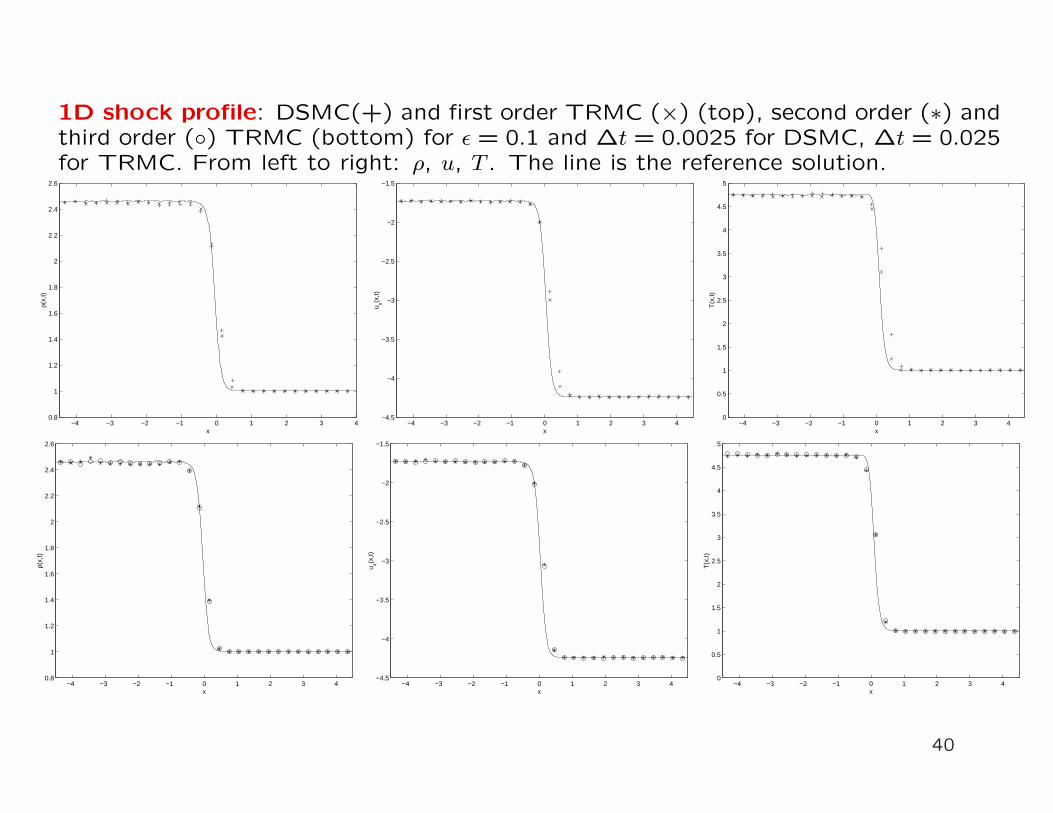
1D shock profile: DSMC(+) and first order TRMC (×) (top), second order (∗) andthird order () TRMC (bottom) for ε = 0.1 and ∆t = 0.0025 for DSMC, ∆t = 0.025for TRMC. From left to right: ρ, u, T . The line is the reference solution.
−4 −3 −2 −1 0 1 2 3 40.8
1
1.2
1.4
1.6
1.8
2
2.2
2.4
2.6
x
ρ(x,
t)
−4 −3 −2 −1 0 1 2 3 4−4.5
−4
−3.5
−3
−2.5
−2
−1.5
x
u x(x,t)
−4 −3 −2 −1 0 1 2 3 40
0.5
1
1.5
2
2.5
3
3.5
4
4.5
5
x
T(x
,t)
−4 −3 −2 −1 0 1 2 3 40.8
1
1.2
1.4
1.6
1.8
2
2.2
2.4
2.6
x
ρ(x,
t)
−4 −3 −2 −1 0 1 2 3 4−4.5
−4
−3.5
−3
−2.5
−2
−1.5
x
u x(x,t)
−4 −3 −2 −1 0 1 2 3 40
0.5
1
1.5
2
2.5
3
3.5
4
4.5
5
x
T(x
,t)
40
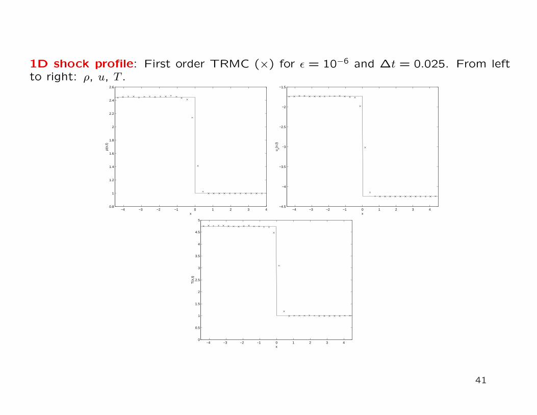
1D shock profile: First order TRMC (×) for ε = 10−6 and ∆t = 0.025. From leftto right: ρ, u, T .
−4 −3 −2 −1 0 1 2 3 40.8
1
1.2
1.4
1.6
1.8
2
2.2
2.4
2.6
x
ρ(x,
t)
−4 −3 −2 −1 0 1 2 3 4−4.5
−4
−3.5
−3
−2.5
−2
−1.5
x
u x(x,t)
−4 −3 −2 −1 0 1 2 3 40
0.5
1
1.5
2
2.5
3
3.5
4
4.5
5
x
T(x
,t)
41
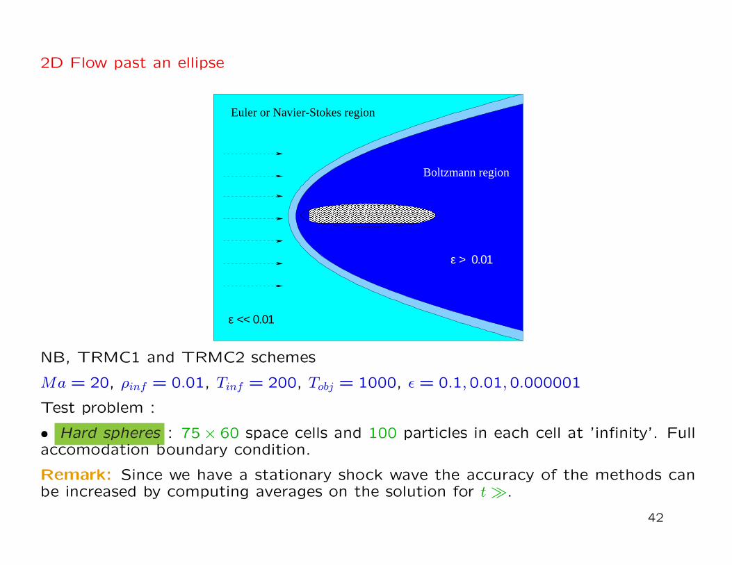
2D Flow past an ellipse
Euler or Navier-Stokes region
Boltzmann region
ε << 0.01
ε > 0.01
NB, TRMC1 and TRMC2 schemes
Ma = 20, ρinf = 0.01, Tinf = 200, Tobj = 1000, ε = 0.1,0.01,0.000001
Test problem :
• Hard spheres : 75× 60 space cells and 100 particles in each cell at ’infinity’. Fullaccomodation boundary condition.
Remark: Since we have a stationary shock wave the accuracy of the methods canbe increased by computing averages on the solution for t À.
42
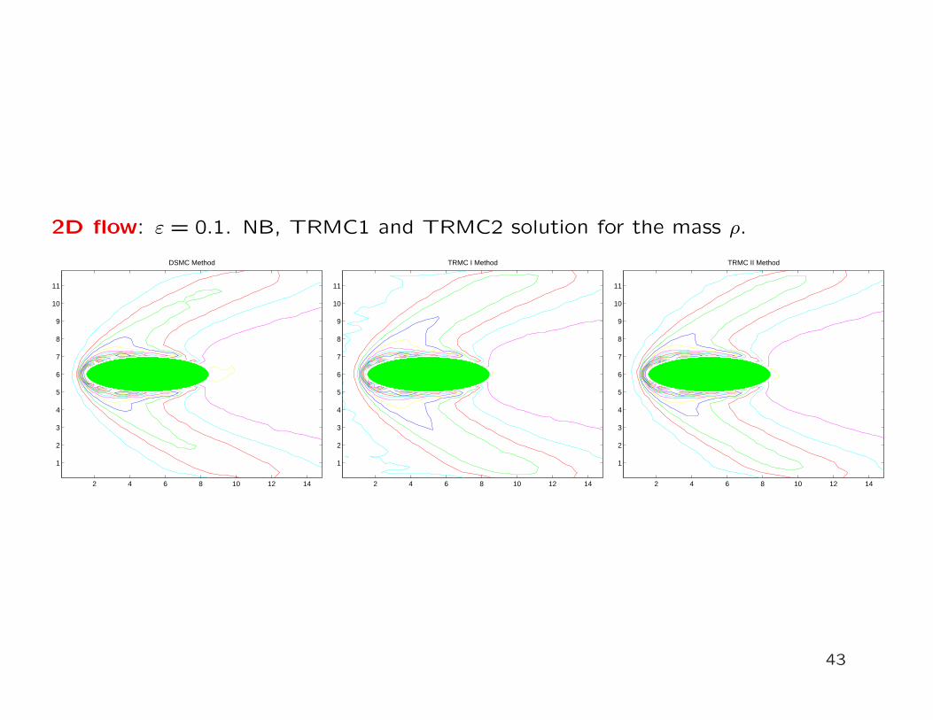
2D flow: ε = 0.1. NB, TRMC1 and TRMC2 solution for the mass ρ.
2 4 6 8 10 12 14
1
2
3
4
5
6
7
8
9
10
11
DSMC Method
2 4 6 8 10 12 14
1
2
3
4
5
6
7
8
9
10
11
TRMC I Method
2 4 6 8 10 12 14
1
2
3
4
5
6
7
8
9
10
11
TRMC II Method
43
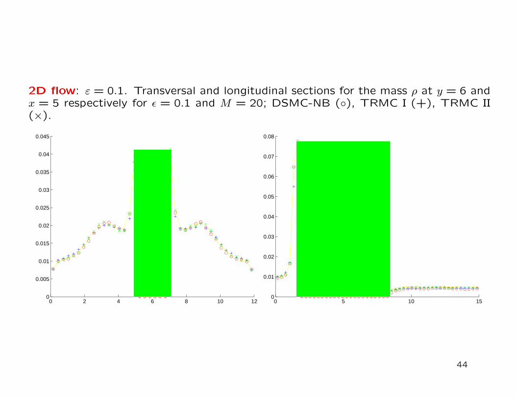
2D flow: ε = 0.1. Transversal and longitudinal sections for the mass ρ at y = 6 andx = 5 respectively for ε = 0.1 and M = 20; DSMC-NB (), TRMC I (+), TRMC II(×).
0 2 4 6 8 10 120
0.005
0.01
0.015
0.02
0.025
0.03
0.035
0.04
0.045
0 5 10 150
0.01
0.02
0.03
0.04
0.05
0.06
0.07
0.08
44
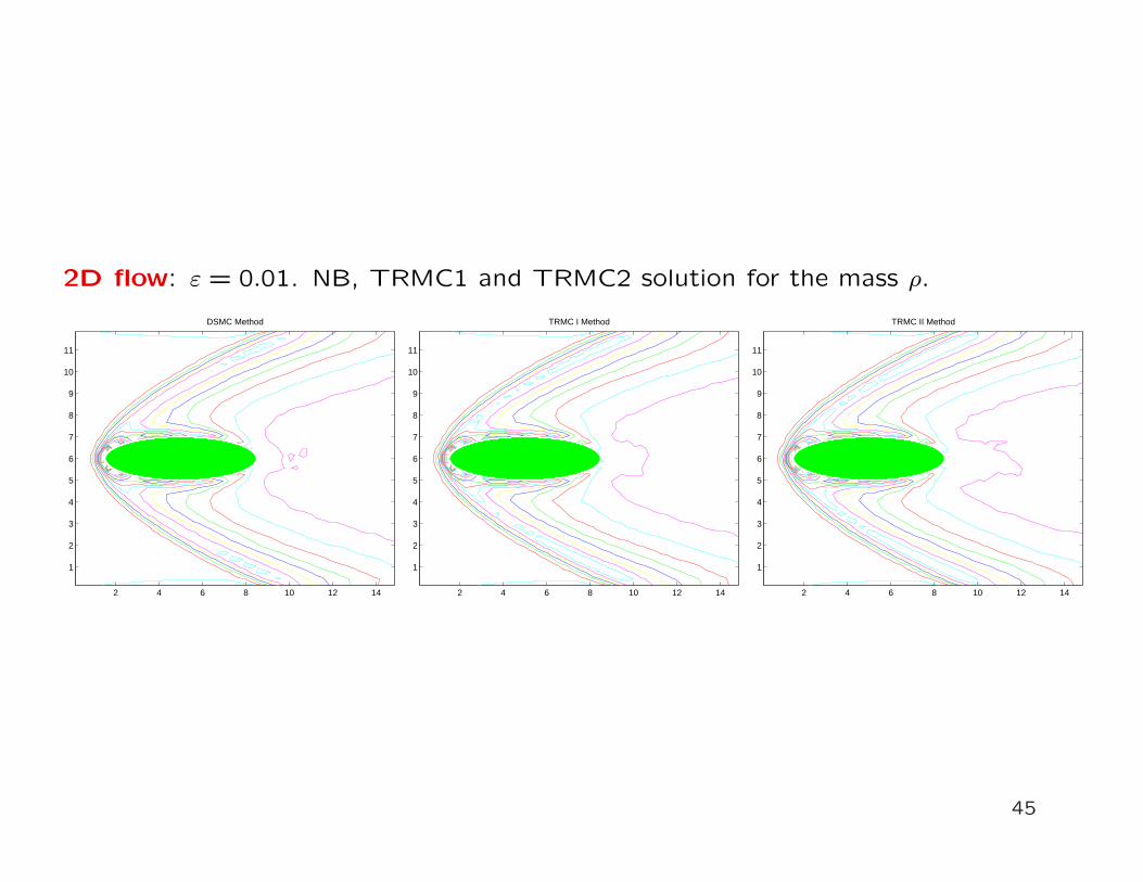
2D flow: ε = 0.01. NB, TRMC1 and TRMC2 solution for the mass ρ.
2 4 6 8 10 12 14
1
2
3
4
5
6
7
8
9
10
11
DSMC Method
2 4 6 8 10 12 14
1
2
3
4
5
6
7
8
9
10
11
TRMC I Method
2 4 6 8 10 12 14
1
2
3
4
5
6
7
8
9
10
11
TRMC II Method
45
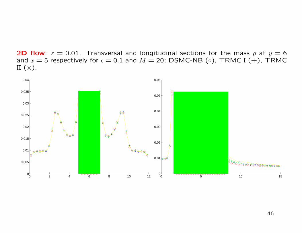
2D flow: ε = 0.01. Transversal and longitudinal sections for the mass ρ at y = 6and x = 5 respectively for ε = 0.1 and M = 20; DSMC-NB (), TRMC I (+), TRMCII (×).
0 2 4 6 8 10 120
0.005
0.01
0.015
0.02
0.025
0.03
0.035
0.04
0 5 10 150
0.01
0.02
0.03
0.04
0.05
0.06
46
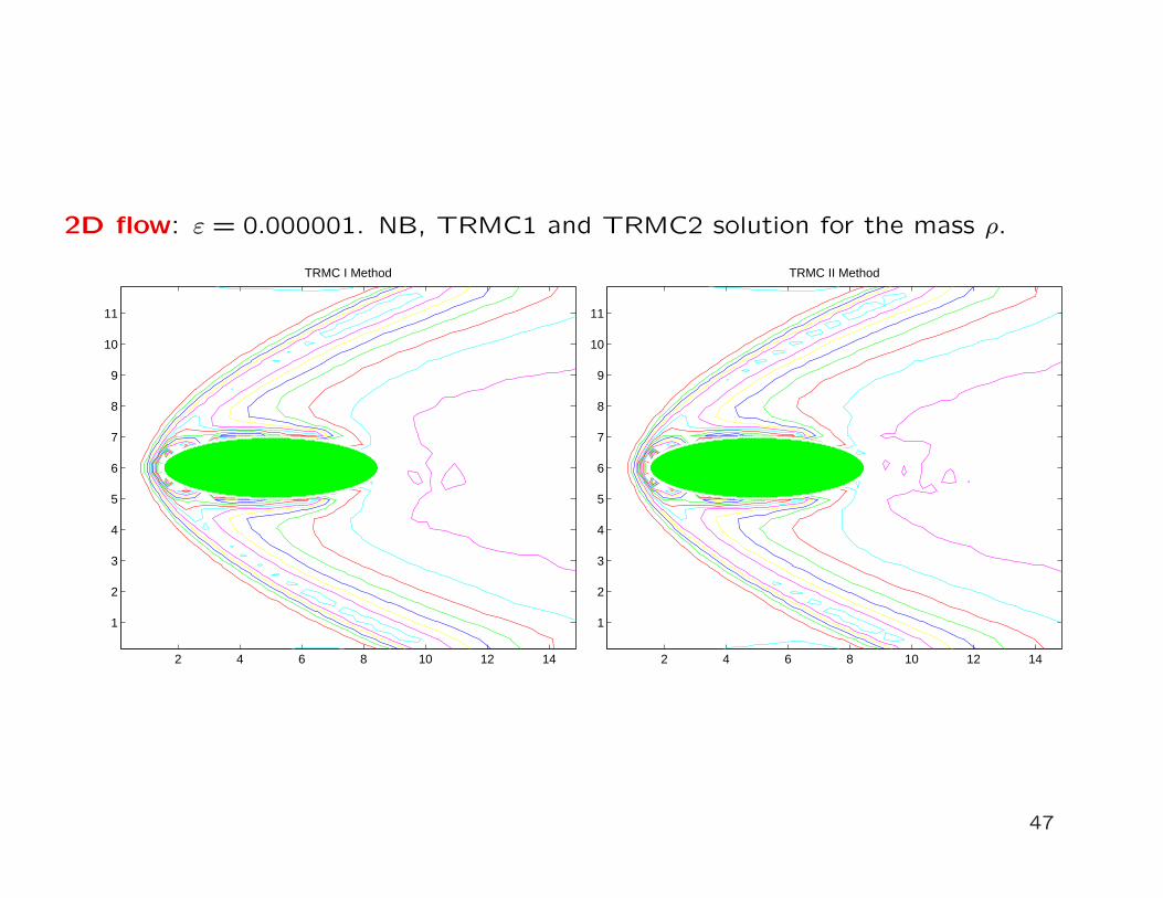
2D flow: ε = 0.000001. NB, TRMC1 and TRMC2 solution for the mass ρ.
2 4 6 8 10 12 14
1
2
3
4
5
6
7
8
9
10
11
TRMC I Method
2 4 6 8 10 12 14
1
2
3
4
5
6
7
8
9
10
11
TRMC II Method
47
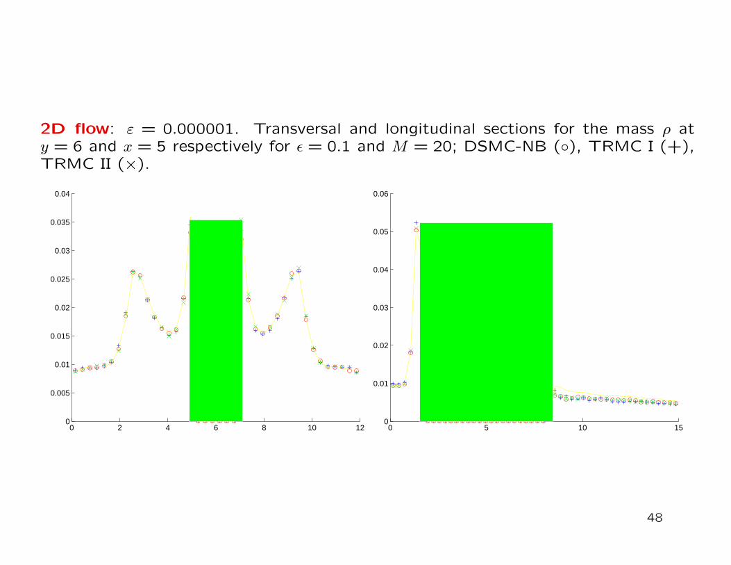
2D flow: ε = 0.000001. Transversal and longitudinal sections for the mass ρ aty = 6 and x = 5 respectively for ε = 0.1 and M = 20; DSMC-NB (), TRMC I (+),TRMC II (×).
0 2 4 6 8 10 120
0.005
0.01
0.015
0.02
0.025
0.03
0.035
0.04
0 5 10 150
0.01
0.02
0.03
0.04
0.05
0.06
48
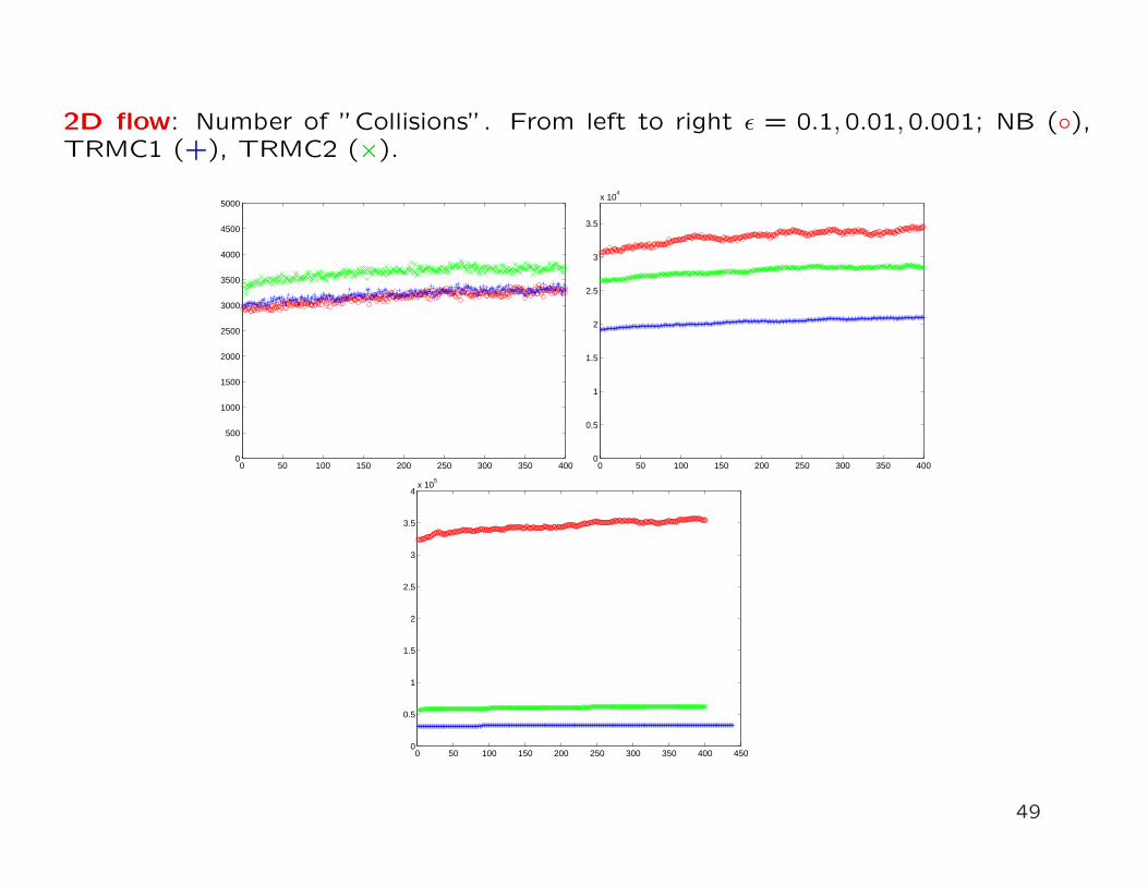
2D flow: Number of ”Collisions”. From left to right ε = 0.1,0.01,0.001; NB (),TRMC1 (+), TRMC2 (×).
0 50 100 150 200 250 300 350 4000
500
1000
1500
2000
2500
3000
3500
4000
4500
5000
0 50 100 150 200 250 300 350 4000
0.5
1
1.5
2
2.5
3
3.5
x 104
0 50 100 150 200 250 300 350 400 4500
0.5
1
1.5
2
2.5
3
3.5
4x 10
5
49
Basic References
[MC] G.A. Bird, Molecular gas dynamics (1994).
[MC] K. Nanbu, J. Phys. Soc. Japan (1983)
[MC] H. Babovsky, Math. Meth. Appl. Sci., (1986).
[MC] H. Babovsky and R. Illner, SIAM J. Numer. Anal., 26 (1989).
[MC] D. I. Pullin, J. Comput. Phys. (1980)
[MC] W. Wagner J.Stat. Phys (1992)
[MC] L.Pareschi, G.Russo, ESAIM Proc. (2001)
[MC,T] L.Pareschi, G.Russo, SIAM J. Sci. Comp. (2001)
[MC,T] L.Pareschi, S.Trazzi, preprint (2003)
[T] E. Gabetta, L. Pareschi, G. Toscani, SIAM J. Numer. Anal. (1997)
Note: TITime discretization, MCIMonte Carlo methods.
50


