Page 1
1
Raspberry Pi Projects for Schools
Project Weather Station
Nathan Taylor
BSc. Computer Science
April, 2014
This document is a project report for a third year project completed in
the School of Computer Science at the University of Manchester.
Supervisor: Dr. James Garside
Page 2
2
Abstract
Raspberry Pi Projects for Schools
Project Weather Station
Nathan Taylor
April, 2014
Supervisor: Dr. James Garside
The United Kingdom is home to some of the most innovative digital industries in the world. However, due to the
general lack of computing skills and knowledge possessed by school leavers and graduates businesses are
concerned, and firms ranging from Advertising to Formula One are struggling to recruit suitable candidates. This is
a problem that not only effects school leavers and graduates that are searching for jobs, but also has an impact on the
growth and development of the creative industries and the technology sector, as well as the country itself.
The problem is caused, in part, by the ICT curriculum that was being taught in schools. Informal learning through
after-school clubs and workshops has arisen to help fill the computing gap and has gained popularity. The purpose
of this project is to boost this popularity, promote further interest in Computer Science and help fill the knowledge
gap.
This report defines the reason and purpose of the project as a tool for both teaching and promoting interest in
Computer Science, and looks at the why the project was undertaken in the first place. It goes on to explore the focus
of the project and why a weather station was chosen. The technology involved is then looked at in detail, and the
development of the project is examined and explained. The report then looks at the results of the project and the
output that is generated by it. Finally, the competed work is considered and concludes that the project achieves the
goals that it set out to at the beginning.
Page 3
3
Acknowledgements
I would like to thank my supervisor, Dr. James Garside, for the help, support and time that he provided over the
course of the project. Whenever faced with a question or problem his thoughts were very much appreciated, as was
his role as a sounding board for my ideas.
I would also like to thank both Dr. James Garside and Dr. Milan Mihajlovic, who acted as my second marker, for the
feedback they provided throughout the year.
Page 4
4
Table of Contents Abstract.......................................................................................................................................................................... 2
Acknowledgements ....................................................................................................................................................... 3
I. Introduction ................................................................................................................................................................ 6
A. Why do this in the first place? .............................................................................................................................. 6
B. Weather stations and why a weather station. ........................................................................................................ 8
II. Design and Technology ............................................................................................................................................ 9
A. Raspberry Pi: I/O, I2C, SPI ................................................................................................................................. 10
i. GPIO ................................................................................................................................................................ 11
ii. I2C ................................................................................................................................................................... 11
iii. SPI ................................................................................................................................................................. 13
B. Setting up the base .............................................................................................................................................. 16
C. Sensors ................................................................................................................................................................ 17
i. BMP085 - Temperature and air pressure ......................................................................................................... 17
ii. DHT22 - Temperature and humidity .............................................................................................................. 18
iii. TGS2600 - General air quality ...................................................................................................................... 18
iv. HMC5883L - Digital compass ....................................................................................................................... 19
v. Anemometer .................................................................................................................................................... 20
vi. Wind Direction .............................................................................................................................................. 22
III. Development .......................................................................................................................................................... 23
A. Base Module ....................................................................................................................................................... 23
B. DHT22 Module - Humidity and Temp ............................................................................................................... 27
C. BMP085 Module - Pressure and Temp ............................................................................................................... 29
D. HMC5883L Module - 3-Axis Digital Compass ................................................................................................. 31
E. TGS 2600 Module - General air quality ............................................................................................................. 33
F. Anemometer Module .......................................................................................................................................... 35
G. Wind Vane Module ............................................................................................................................................ 36
IV. Evaluation and Results .......................................................................................................................................... 39
A. Calibration .......................................................................................................................................................... 39
Page 5
5
i. BMP085 ........................................................................................................................................................... 39
ii. TGS 2600 ........................................................................................................................................................ 40
iii. HMC5883L.................................................................................................................................................... 40
iv. Anemometer .................................................................................................................................................. 42
B. Sensor Output ..................................................................................................................................................... 42
V. Conclusion (1,500) ................................................................................................................................................. 46
A. Summary ............................................................................................................................................................ 46
B. Expansion ........................................................................................................................................................... 48
i. Light levels ...................................................................................................................................................... 48
ii. Cloud detection ............................................................................................................................................... 48
iii. Rain detection ................................................................................................................................................ 48
iv. Rain gauge ..................................................................................................................................................... 49
C. Critique ............................................................................................................................................................... 50
VI. References ............................................................................................................................................................. 51
VII. Figures .................................................................................................................................................................. 52
Page 6
6
I. Introduction
This section of the report introduces the general premise of the project, look at some of the difficulties that were
encountered, examine the ‘why’ behind the project in the first place and, finally, show some of the reasons that it
became Raspberry Pi Projects for Schools: Project Weather Station.
The purpose of the project was to develop something modular that could be used to teach school children about
various aspects of Computer Science, such as programming, experimentation and problem solving. The project had
to be large enough in scope to produce meaningful results, but able to be broken down into sections or modules that
could be completed separately. After the platform is setup the modules can be completed in any order, with a
noticeable result when completing each module. The purpose of this is to not overwhelm, but to create manageable
parts that are, hopefully, engaging and to produce an outcome at the end that can be observed.
Due to the nature of the project it includes hardware interaction in the form of assembling the components and
attaching them to the Raspberry Pi, software interaction through programming languages such as Python and C to
drive these components and receive some output, and some basic construction for the custom built sensors.
Why do this in the first place?
The reason for the project, and other Raspberry Pi projects, is to address what is currently being taught in schools,
and the general lack of computing skills in the United Kingdom. This country is home to some of the most
innovative digital industries in the world, and yet there is a lack of competent students and as a result the
employment needs of high-tech and creative businesses are failing to be met. This is leaving businesses and firms in
the United Kingdom concerned over the lack of school-leaver and graduate computing skills, with firms in sectors
from Advertising to Formula One struggling to recruit. This does not just hurt the school-leavers and graduates
looking for jobs, but also hurts the growth and development of the technological industries and creative businesses
as well as the country as a whole.
Part of the problem stems from the current ICT curriculum, which has been described by Michael Gove as “a mess
that must be radically revamped to prepare pupils for the future”1. It has also been described as a dull, off-putting,
demotivating and irrelevant curriculum that fails to inspire students by industry leaders and teachers, as well as the
British Computer Society and the National Association of Advisors for Computers in Education (NAACE).2
This problem with the ICT curriculum leads to very low numbers of students taking Computing at A-level across the
country. Statistics from the Department of Education show that only 0.4% of the A-levels taken in 2012 were
Computing, a number that has been declining every year since 1998. This indicates that a large number of students
that go on to higher education to read a computing topic have not completed a Computing A-level, which means an
Page 7
7
even less formal background in computer science than those that have. This only adds to the claims that computing
and programming skills are not being adequately provided.
Change is on the way, however, with a new computer science-based ICT curriculum launched by the Department of
Education to replace the old, outdated ICT curriculum in September 2014. To go along with this new Computer
Science GCSEs have been developed by all of the major examining bodies and the Department of Education is
considering adding Computer Science as a ‘Fourth Science’ to the English-Baccalaureate.
There are other barriers that must also be overcome, such as the lack of qualified teachers. According to the Royal
Society two thirds of teachers are not deemed to have sufficiently relevant qualifications to teach the existing ICT
courses, let alone the new proposed Computer Science course. As with all STEM subjects thought must also be
given to the gender divide, for 2011/2012 only 7% of Computing A-level students were girls.
Further support for hobbyist learning and a network of after-school clubs should also be considered. Due to the poor
state of the ICT curriculum there has been a rise in interest in informal learning through things like hackathon days
and workshops for devices such as the Arduino and Raspberry Pi.4,5,6 These events have been hugely popular and
have helped to promote interest in Computer Science and show how much potential there is. They have also shown
how accessible and affordable these platforms are and how much can be done with them, whether a beginner or an
expert.
Page 8
8
Weather stations and why a weather station.
As the project is aimed at school children it was felt that it needed to be big enough to be broken down into sections,
with the completion of each section producing a result, but the sections also had to tie in together to produce a
cohesive final product. Additionally, being able to use the project to teach about other subjects would be a bonus.
These requirements were the basis of the research as to what should actually be built. A DIY weather station was
one of the first ideas that was considered and eventually seemed the best fit for the requirements, easily allowing for
the modular and interdisciplinary approach that was wanted.
However, before committing to the idea of a weather station research was done to determine how viable it would be.
This was due to the complexity of weather stations and the atmospheric conditions that they measure and use, such
as: wind speed, wind direction, temperature, humidity, air pressure, visibility, rain fall, light levels, air quality, etc.
Information that is then used to provide weather forecasts.
Despite the complexity, it was found that off-the-shelf sensors were available that would provide data for most of
these atmospheric conditions and it would be possible to custom build sensors for the rest. Other projects and
articles online showed that interfacing these sensors, or sensors like them, with the Raspberry Pi was possible. This
showed that the Raspberry Pi was a suitable platform for the project and it was determined that the project was
indeed feasible.
Page 9
9
II. Design and Technology
This part of the report is about the research and design of the project, and the sensors that were used. The sensors are
explored in more technical detail, as is the Raspberry Pi.
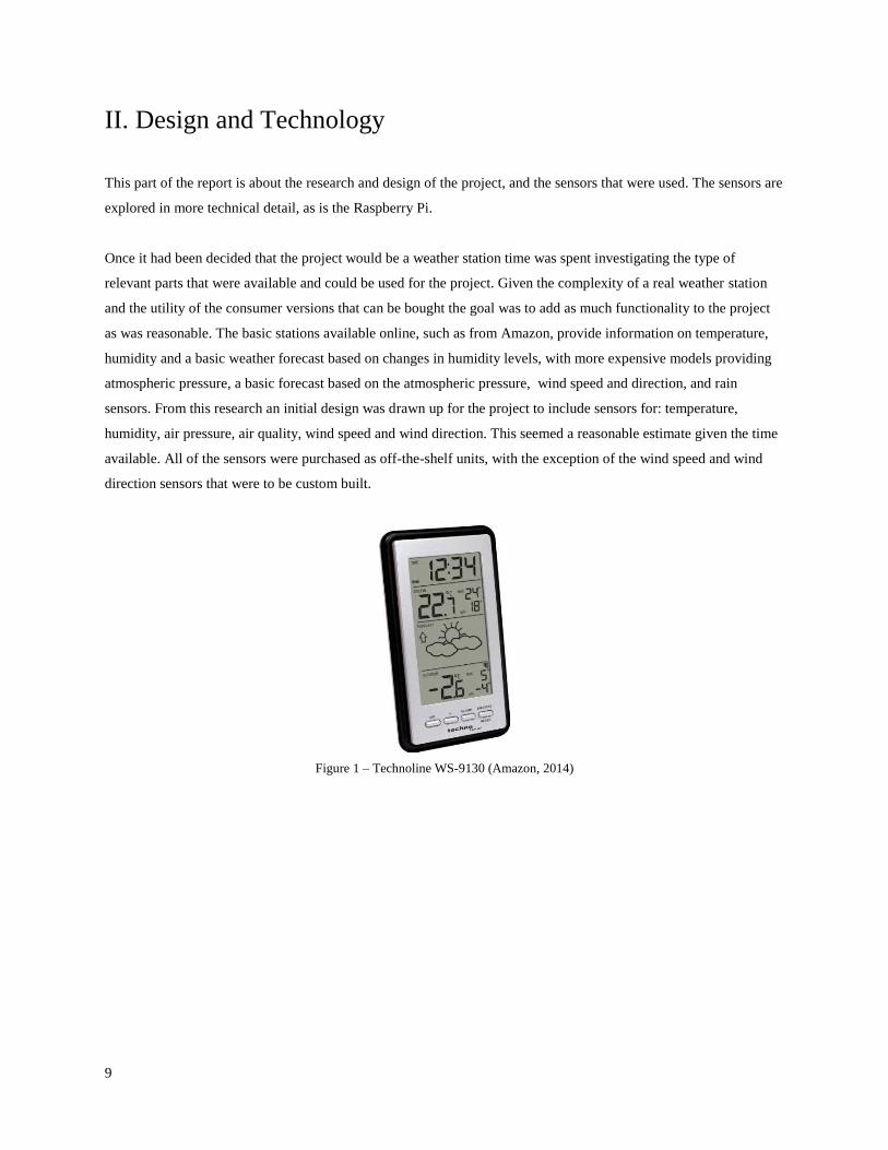
Once it had been decided that the project would be a weather station time was spent investigating the type of
relevant parts that were available and could be used for the project. Given the complexity of a real weather station
and the utility of the consumer versions that can be bought the goal was to add as much functionality to the project
as was reasonable. The basic stations available online, such as from Amazon, provide information on temperature,
humidity and a basic weather forecast based on changes in humidity levels, with more expensive models providing
atmospheric pressure, a basic forecast based on the atmospheric pressure, wind speed and direction, and rain
sensors. From this research an initial design was drawn up for the project to include sensors for: temperature,
humidity, air pressure, air quality, wind speed and wind direction. This seemed a reasonable estimate given the time
available. All of the sensors were purchased as off-the-shelf units, with the exception of the wind speed and wind
direction sensors that were to be custom built.
Figure 1 – Technoline WS-9130 (Amazon, 2014)
Page 10
10
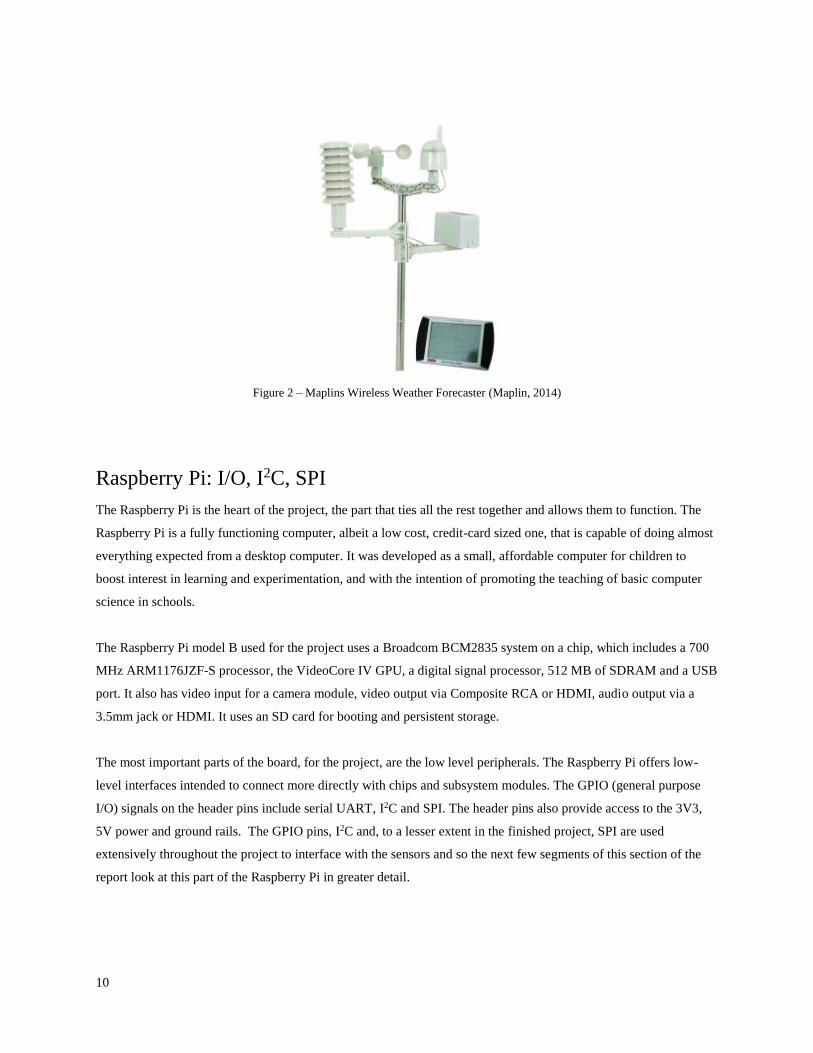
Figure 2 – Maplins Wireless Weather Forecaster (Maplin, 2014)
Raspberry Pi: I/O, I2C, SPI
The Raspberry Pi is the heart of the project, the part that ties all the rest together and allows them to function. The
Raspberry Pi is a fully functioning computer, albeit a low cost, credit-card sized one, that is capable of doing almost
everything expected from a desktop computer. It was developed as a small, affordable computer for children to
boost interest in learning and experimentation, and with the intention of promoting the teaching of basic computer
science in schools.
The Raspberry Pi model B used for the project uses a Broadcom BCM2835 system on a chip, which includes a 700
MHz ARM1176JZF-S processor, the VideoCore IV GPU, a digital signal processor, 512 MB of SDRAM and a USB
port. It also has video input for a camera module, video output via Composite RCA or HDMI, audio output via a
3.5mm jack or HDMI. It uses an SD card for booting and persistent storage.
The most important parts of the board, for the project, are the low level peripherals. The Raspberry Pi offers low-
level interfaces intended to connect more directly with chips and subsystem modules. The GPIO (general purpose
I/O) signals on the header pins include serial UART, I2C and SPI. The header pins also provide access to the 3V3,
5V power and ground rails. The GPIO pins, I2C and, to a lesser extent in the finished project, SPI are used
extensively throughout the project to interface with the sensors and so the next few segments of this section of the
report look at this part of the Raspberry Pi in greater detail.
Page 11
11
GPIO
General Purpose Input/Output is a generic pin on a chip the behaviour of which can be programmed through
software, including whether it is an output or input pin. The Raspberry Pi allows peripherals and expansion boards
to access the CPU by exposing the inputs and outputs. It has a 26-pin GPIO expansion header arranged in a 2x13
strip, which provides 8 GPIO pins, access to I2C, SPI, UART as well as 3.3V, 5V and GND supply lines.
All the GPIO pins can be reconfigured to provide alternate functions such as SPI, PWM (pulse width modulation,
I2C and so on. At reset pins GPIO 14 and 15 are assigned by default to the alternate function UART, though these
can be switched back to GPIO to provide more GPIO pins. Each GPIO can interrupt, and can detect high state, low
state, rising-edge, falling-edge and state change. A recent patch for the recommended operating system for the
Raspberry Pi, a custom version of the Debian Linux distribution called Raspbian, has added support for GPIO
interrupts to the kernel.
I2C
I2C stands for Inter-Integrated Circuit. It is a multimaster serial single-ended computer bus that is used for attaching
low-speed peripherals to a motherboard, microcontroller, mobile phone or other digital electronic devices.7
I2C uses only two bidirectional open-drain lines, the Serial Data Line (SDA) and the Serial Clock Line (SCL), both
pulled up with resistors. Typical voltages used are 3V3 or 5V, though systems with other voltages are permitted.
Reference design
The I2C reference design is a bus with a clock (SCL) and data (SDA) lines with 7-bit addressing. The bus has two
roles that nodes can take: master and slave. A master node is a node that generates the clock and initiates
communication with slaves. A slave node is a node that receives the clock and responds when addressed by the
master. I2C is a multimaster bus, this means that any number of master nodes can be present. Master and slave roles
may also be changed between messages, after a STOP is sent.
Each bus device has four potential modes of operation, two for each role: master and slave. Most devices will only
use a single role and its two associated modes.
● Master transmit - master node sending data to a slave
● Master receive - master node receiving data from a slave
● Slave transmit - slave node sending data to the master
● Slave receive - slave node receiving data from the master
The master is initially in master transmit mode, and starts by sending a start bit followed by the 7-bit address of the
slave it wants to communicate with, followed by a single bit representing whether it wants to write(0) to or read(1)
from the slave.
Page 12
12
If the slave exists on the bus it will respond with an ACK bit (active low for acknowledged) for that address. The
master then continues in either transmit or receive mode, and the slave continues in its complementary mode.
The address and the data bytes are sent most significant bit first. The START bit is indicated by a high-to-low
transition of SDA with SCL high; the STOP bit is indicated by a low-to-high transition of SDA with SCL high. All
other transitions of SDA take place with SCL low.
If the master wishes to write to the slave then it repeatedly sends a byte with the slave sending an ACK bit.
If the master wishes to read from the slave then it repeatedly receives a byte from the slave, the master sending an
ACK bit after every byte but the last one.
The master then either ends transmission with a STOP bit, or it may send another START bit if it wishes to retain
control of the bus for another transfer (a "combined message").
In a combined message, each read or write begins with a START and the slave address. After the first START these
are called repeated START bits, and they are not preceded by STOP bits. In this way, the slave knows the next
transfer is part of the same message.
Message protocols
I2C defines basic message types, each of which begins with a START and ends with a STOP:
● Single message where a master writes data to a slave.
● Single message where a master reads data from a slave.
● Combined messages, where a master issues at least two reads and/or writes to one or more slaves.
Page 13
13
Timing diagram
Figure 3 – I2C Data transfer sequence (Wikipedia, 2014)
1. Data transfer is initiated with a START bit (S) signaled by SDA being pulled low while SCL stays
high. SCL is subsequently pulled low, also.
2. SDA sets the 1st data bit level while keeping SCL low (during blue bar time) and the data is
sampled (received) when SCL rises (green).
3. When the transfer is complete, a STOP bit (P) is sent by releasing the clock first and then the data
line to allow it to be pulled high while SCL is kept high continuously.
4. To avoid false marker detection, the level on SDA is changed after the SCL falling edge and is
sampled and captured on the rising edge of SCL.
SPI
SPI stands for Serial Peripheral Interface, it is a synchronous serial data link bus that operates in full duplex mode.8
It is used for short distance, single master communication, usually in embedded systems, sensors and SD cards.
While no longer used in the current stage of the project, it was experimented with early on before I2C became the
main bus used by the majority of the sensors.
In SPI, devices communicate in master/slave mode where the master device initiates the data frame. Multiple slaves
are allowed with individual slave select lines.
The SPI bus specifies four logic signals:
● SCLK: Serial Clock - output from master.
● MOSI: Master Output, Slave Input - output from master.
● MISO: Master Input, Slave Output - output from slave
● SS: Slave Select - active low, output from master.
The SPI bus can operate with a single master device and with one or more slave devices. If a single slave device is
used, the SS pin may be fixed to logic low if the slave permits it. With multiple slave devices, an independent SS
signal is required from the master to each slave device.
Page 14
14
Data transmission
To begin a communication, the bus master first configures the clock using a frequency less than or equal to the
maximum frequency the slave device supports. The master then asserts the logic 0 for the desired chip over the chip
select line, this is because the chip select line is active low. If a waiting period is required the master must wait at
least that period before starting to issue clock cycles.
A full duplex data transmission occurs during each SPI clock cycle:
● the master sends a bit on the MOSI line which is read by the slave
● the slave sends a bit on the MISO line which is read by the master
Figure 4 –SPI data transmission,
two shift registers form an interchip circular buffer (Wikipedia, 2014)
Transmissions may involve any number of clock cycles. When there is no more data to be transmitted the master
stops toggling its clock, and then deselects the slave.
The master must also configure the clock polarity and phase with respect to the data, the adopted convention names
these CPOL and CPHA respectively.
Page 15
15
Timing diagram
Figure 5 – SPI timing diagram showing clock polarity and phase (Wikipedia, 2014)
At CPOL=0 the base value of the clock is zero
● For CPHA=0, data are captured on the clock's rising edge (low→high transition) and data is
propagated on a falling edge (high→low clock transition).
● For CPHA=1, data are captured on the clock's falling edge and data is propagated on a rising edge.
At CPOL=1 the base value of the clock is one (inversion of CPOL=0)
● For CPHA=0, data are captured on clock's falling edge and data is propagated on a rising edge.
● For CPHA=1, data are captured on clock's rising edge and data is propagated on a falling edge.
CPHA=0 means sample on the leading (first) clock edge, while CPHA=1 means sample on the trailing (second)
clock edge, regardless of whether that clock edge is rising or falling.
Page 16
16
Setting up the base
As mentioned above, the plan was to have each sensor form its own ‘module’, but before this was possible there
needed to be a base ‘module’ or platform to which to add them. This base module serves a two-fold purpose, it sets
up a base for the project to allow for the addition of the modules and it introduces the user to the hardware and
software that will be used.
The base includes all of the vital parts that project needs to function: the Raspberry Pi, a breadboard used as the
construction base, a GPIO connector from the Raspberry Pi to the breadboard, various jumper wires, resistors and
LEDs for testing. The user is taken through setting up the components, connecting the LEDs, manipulating the
GPIO pins and turning on the LEDs using the Python programming language.
Figure 6 – Assorted base module parts (Nathan Taylor, 2014)
Page 17
17
Sensors
The sensors are the core of the project and the ones that are used provide readings for temperature, humidity, air
pressure, altitude, air quality, direction, wind speed and wind direction. The sections below look at each of the
sensors in greater detail.
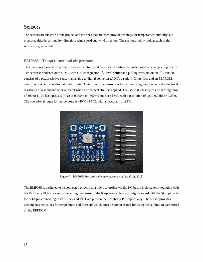
BMP085 - Temperature and air pressure
This measures barometric pressure and temperature, and provides an altitude estimate based on changes in pressure.
The sensor is soldered onto a PCB with a 3.3V regulator, I2C level shifter and pull-up resistors on the I2C pins. It
consists of a piezoresistive sensor, an analog to digital converter (ADC), a serial I2C interface and an EEPROM
control unit which contains calibration data. A piezoresistive sensor works by measuring the change in the electrical
resistivity of a semiconductor or metal when mechanical strain is applied. The BMP085 has a pressure sensing range
of 300 to 1,100 hectopascals (hPa) or 9,000m to -500m above sea level, with a resolution of up to 0.03hPa / 0.25m.
The operational range for temperature is -40°C - 85°C, with an accuracy of ±2°C.
Figure 7 – BMP085 Pressure and temperature sensor (Adafruit, 2013)
The BMP085 is designed to be connected directly to a microcontroller via the I2C bus, which makes integration with
the Raspberry Pi fairly easy. Connecting the sensor to the Raspberry Pi is also straightforward with the SCL pin and
the SDA pin connecting to I2C Clock and I2C Data pins on the Raspberry Pi, respectively. The sensor provides
uncompensated values for temperature and pressure which must be compensated for using the calibration data stored
on the EEPROM.
Page 18
18
DHT22 - Temperature and humidity
The DHT22 is a basic, low-cost digital temperature and humidity sensor. It works through the use of a thermistor
and a capacitive humidity sensor. A thermistor is a type of resistor whose resistance varies significantly with
temperature, and the capacitive humidity sensor works by measuring the effect of humidity on the dielectric constant
of a metal oxide material. The sensor measures humidity readings between 0 to 100% humidity with an accuracy of
between 2 - 5% and temperature readings of -40°C - 80°C with an accuracy of ±0.5°C, it then outputs a digital
signal on the data pin. The sensor requires careful timing to retrieve the data and a low sampling rate of 0.5 Hz
means that new data can only be retrieved once every two seconds.
Figure 8 – DHT22 Temperature and humidity sensor (Adafruit, 2014)
The sensor is temperature compensated and calibrated in an accurate calibration chamber and the calibration-
coefficient data is saved in one-time programmable memory. The sensor has four pins, but only three of them are
used to connect it to the microcontroller. It uses a single I/O comms wire with a non-standard interface, which is pin
2, the data pin.
TGS2600 - General air quality
The TGS 2600 is a general air quality sensor, it has a high sensitivity to low concentrations of gaseous air
contaminants such as hydrogen and carbon monoxide and can detect hydrogen at a level of several ppm. The sensing
element is made up of a metal oxide semiconductor layer formed on an alumina substrate of a sensing chip together
with an integrated heater. The integrated heater maintains the sensing unit at a specific temperature optimal for
sensing.
When in the presence of detectable gas, the conductivity of the sensor increases depending on the concentration of
the gas and an electrical circuit can be used to convert the change in conductivity to an output signal which gives a
measure of the gas concentration.
Page 19
19
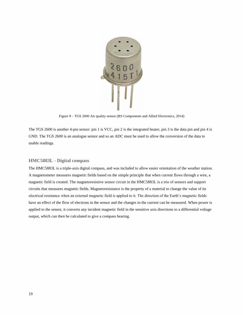
Figure 9 – TGS 2600 Air quality sensor (RS Components and Allied Electronics, 2014)
The TGS 2600 is another 4-pin sensor: pin 1 is VCC, pin 2 is the integrated heater, pin 3 is the data pin and pin 4 is
GND. The TGS 2600 is an analogue sensor and so an ADC must be used to allow the conversion of the data to
usable readings.
HMC5883L - Digital compass
The HMC5883L is a triple-axis digital compass, and was included to allow easier orientation of the weather station.
A magnetometer measures magnetic fields based on the simple principle that when current flows through a wire, a
magnetic field is created. The magnetoresistive sensor circuit in the HMC5883L is a trio of sensors and support
circuits that measures magnetic fields. Magnetoresistance is the property of a material to change the value of its
electrical resistance when an external magnetic field is applied to it. The direction of the Earth’s magnetic fields
have an effect of the flow of electrons in the sensor and the changes in the current can be measured. When power is
applied to the sensor, it converts any incident magnetic field in the sensitive axis directions to a differential voltage
output, which can then be calculated to give a compass bearing.
Page 20
20
Figure 10 – HMC5883L 3-Axis digital compass (Adafruit, 2014)
The sensor has an integrated 12-bit ADC and is designed to connect directly via the I2C bus, which makes its use
relatively simple. It has a ±2 degree heading accuracy and a range of -8 to +8 gauss. Gauss is the cgs (centimetre-
gram-second) unit of measurement of a magnetic field B, also known as the “magnetic flux density” or the
“magnetic induction”. The Earth’s magnetic field at its surface is 0.31 to 0.58 gauss. Connecting the sensor is much
the same as the BMP085, connect VCC to +3-5V, GND to ground, SCL to I2C Clock and SDA to I2C Data.
Anemometer
An anemometer is a device used for measuring wind speed, it is a common instrument on a weather station.
Anemometers can be divided into two classes: those that measure the wind’s speed, and those that measure the
wind’s pressure. There is a close connection between the speed and the pressure, and an anemometer designed to
measure one will give information about both. However, the focus of the sensor being used in the project is on wind
speed.
Hand-held anemometers are widely available online, at reasonable prices, and anemometers that interface with
existing weather station products are also available, but attempting to integrate one of these into the weather station
project would be overly complicated and require a large amount of time and effort. Instead, it was decided that the
anemometer for the project would be a DIY sensor, constructed specifically for the project.
As stated above, the anemometer is a velocity anemometer, more specifically a cup anemometer. A cup anemometer
is a simple type of anemometer that consists of a number of hemispherical cups each mounted on the end of a
horizontal arm, with the arms mounted at equal angles to each other on a vertical shaft. The air flow past the cups in
any horizontal direction turns the shaft proportional to the wind speed. This means that counting the revolutions of
the shaft over a set period time provides an average wind speed.
Page 21
21
Figure 11 – Hemispherical cup anemometer
invented in 1846 by John Robinson (Wikipedia, 2014)
Page 22
22
Wind Direction
Wind direction is reported by the direction from which it originates, a northerly wind blows from north to south, for
example. There are a variety of instruments used to measure the direction of the wind, such as the wind vane and
windsock. Both of which work by moving to minimise air resistance. The way a wind vane is pointed shows the
direction from which the wind is blowing, and with a windsock the larger opening faces the direction the wind is
blowing from and the tail, with the smaller opening, points in the direction the wind is blowing.
Figure 12 – Modern wind vane (APRS World, 2014)
A wind vane is used for the purpose of the project. In its basic form it is a type of arrow mounted on an axle, which
moves by itself. This means that determining the direction of the wind consists of determining the absolute position
of the axle on which the arrow is mounted, though due to the nature of the wind the arrow may “flap” around
somewhat, meaning that some form of smoothing would be required for a more accurate direction reading.
Page 23
23
III. Development
This section of the report focuses on the building of the project, both hardware and software. Taking the information
and design given in the previous section and turning it into a working project.
Base Module
Following the modular approach wanted and detailed in the design, the modules have no particular order in which
they must be completed, with the exception of the base module which must be completed first. This sets up the
platform for the addition of any and all of the other modules.
The base module consists of the Raspberry Pi, the breadboard, jumper wires, some resistors and some LEDs. The
idea is to become familiar with the use of the Raspberry Pi and the breadboard, and experiment with the GPIO pins
and the LEDs.
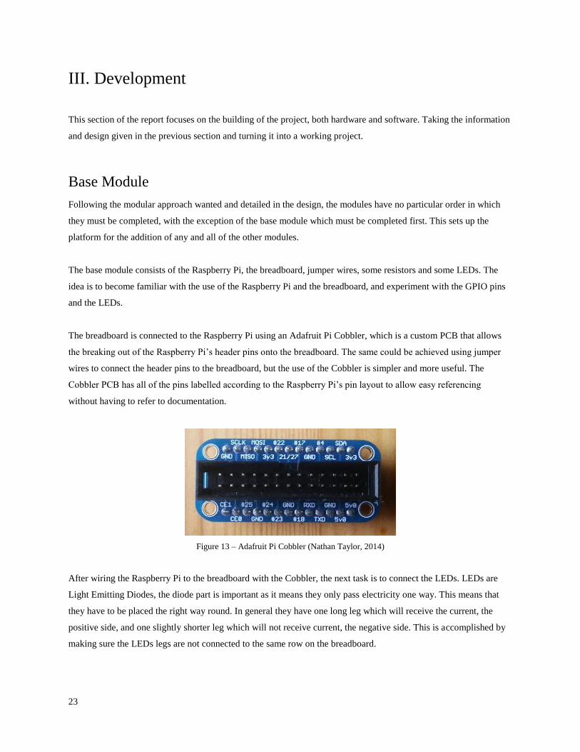
The breadboard is connected to the Raspberry Pi using an Adafruit Pi Cobbler, which is a custom PCB that allows
the breaking out of the Raspberry Pi’s header pins onto the breadboard. The same could be achieved using jumper
wires to connect the header pins to the breadboard, but the use of the Cobbler is simpler and more useful. The
Cobbler PCB has all of the pins labelled according to the Raspberry Pi’s pin layout to allow easy referencing
without having to refer to documentation.
Figure 13 – Adafruit Pi Cobbler (Nathan Taylor, 2014)
After wiring the Raspberry Pi to the breadboard with the Cobbler, the next task is to connect the LEDs. LEDs are
Light Emitting Diodes, the diode part is important as it means they only pass electricity one way. This means that
they have to be placed the right way round. In general they have one long leg which will receive the current, the
positive side, and one slightly shorter leg which will not receive current, the negative side. This is accomplished by
making sure the LEDs legs are not connected to the same row on the breadboard.
Page 24
24
Figure 14 – Raspberry Pi connected to breadboard via Pi Cobbler (Nathan Taylor, 2014)
If too much current is allowed though the LED it will burn brightly for a very short time and then burn out. This is
the reason for the resistors, to limit the current flowing to the LED and stop it burning out. Anything from 270 Ohms
and up will be sufficient to limit the current, the higher the resistor value the dimmer the LED will be.
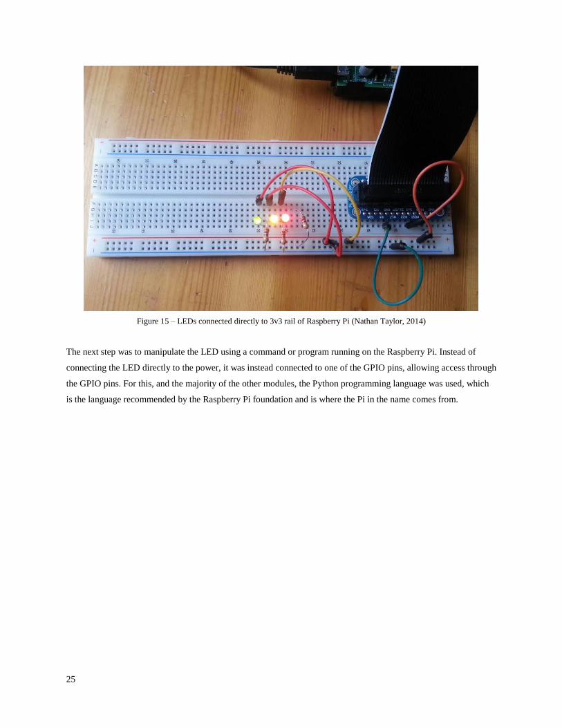
Once the LED and resistor have been connected to the breadboard they are tested, by connecting the positive side of
the LED directly to the 3V3 power rail which will make the LED light up.
Page 25
25
Figure 15 – LEDs connected directly to 3v3 rail of Raspberry Pi (Nathan Taylor, 2014)
The next step was to manipulate the LED using a command or program running on the Raspberry Pi. Instead of
connecting the LED directly to the power, it was instead connected to one of the GPIO pins, allowing access through
the GPIO pins. For this, and the majority of the other modules, the Python programming language was used, which
is the language recommended by the Raspberry Pi foundation and is where the Pi in the name comes from.
Page 26
26
Python has very useful libraries for working with the Raspberry Pi and its GPIO pins, and once they were found
manipulating the LEDs was very easy, as is demonstrated with the following lines of code.
# Import time library so the program can be paused
import time
# Import the R-Pi GPIO libraries that allow us to connect to other devices via
the GPIO pins
import RPi.GPIO as GPIO
# Set the GPIO library to use the R-Pi’s BCM board pin numbers
GPIO.setmode(GPIO.BCM)
# Set pin 18 on the GPIO header to act as an output
GPIO.setup(18, GPIO.OUT)
# Set pin 18 high, turning on the LED
GPIO.output(18, GPIO.HIGH)
# Sleep for 5 seconds
time.sleep(5)
Set pin 18 low, turning off the LED
GPIO.output(18, GPIO.LOW)
This very basic example serves to show the ease with which the GPIO pins and the LEDs can be manipulated with a
little bit of knowledge. The rest of the module involves manipulating multiple LEDs, introducing loops, playing with
the timing for the LEDs, to create traffic lights for example, and printing out messages to the command line when
LEDs are toggled.
A small introduction to the basics the rest of project is based on. This module was designed and completed easily
and quickly while waiting for some of the other parts to arrive.
Page 27
27
DHT22 Module - Humidity and Temp
This module deals with wiring up and receiving an output from the DHT22 temperature and humidity sensor. The
sensor is manufactured by a Chinese company, Aosong Electronics, and is very low-cost. As such it doesn’t use a
standard for communication between it and the microcontroller, but instead uses its own communication protocol.
Connecting the sensor the the Raspberry Pi was straightforward, all that was required was the sensor, some jumper
wires and a 10k Ohm resistor. The pins on the sensor are long enough to allow it to plug directly into the
breadboard. The sensor has four pins: VCC (3 to 5V power), Data out, Null and GND. The pins connect to the
Raspberry Pi and breadboard as expected, VCC to 3V3 power, Data out to a GPIO pin, Null is not connected and
GND to ground. The 10k Ohm resistor is placed between the VCC and the data pin to act as a medium-strength pull
up on the data line.
Figure 16 – DHT22 wiring (Nathan Taylor, 2014)
Once the sensor had been connected work could start on writing a program to get a reading from it. Due to the
delicate timings required for communication with the sensor the C programming language is used, instead of
Python. This is the only part of the project for which this change had to be made.
When the start signal is sent to the sensor, it changes from low-power mode to running mode, and after the start
signal has finished the sensor sends a response signal of 40-bit data that contains the relative humidity and
temperature readings. Data from the sensor is comprised of integral and decimal parts. From the datasheet, DATA =
8 bit integral RH data + 8 bit decimal RH data + 8 bit integral T data + 8 bit decimal T data + 8 bit checksum. As
Page 28
28
can be seen, the sensor outputs 40 bits of data, five lots of 8 bit data; the first two 8 bits contain the relative humidity
data, the second two contain the temperature data and the last chunk of 8 bit data is the checksum. The checksum
should be the last 8 bits of the rest of the data combined.
The start signal is sent to the sensor by pulling the data pin low for 18 milliseconds. The data pin is high by default
because of the pull-up resistor used when wiring the sensor in. The data pin is then pushed high for 40
microseconds. This is the end of the start signal and when it is detected the sensor sends a response signal by pulling
the data pin low for 80 microseconds. The sensor then prepares to send the data, pulling the data pin high for another
80 microseconds. The data is then sent, with every bit’s transmission beginning with the data pin being pulled low
for 50 microseconds. The data pin is then pulled high, with the signal’s length determining whether the bit is “1” or
“0”.
After all the data has been sent, the checksum is verified by comparing the received checksum with the expected
checksum, and if they match then the data can be separated and printed out. Otherwise the data is discarded and
another reading is attempted.
As the rest of the project was completed using the Python programming language, the next part of this module
involved running the C program for this sensor within a Python program, using a regular expression search to find
the temperature and humidity readings in the C program and assign them to variables that could be used in the
Python program. After a lot of research and experimentation with Pythons function and libraries this turn out to be
quite straightforward.
Page 29
29
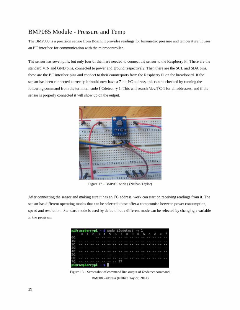
BMP085 Module - Pressure and Temp
The BMP085 is a precision sensor from Bosch, it provides readings for barometric pressure and temperature. It uses
an I2C interface for communication with the microcontroller.
The sensor has seven pins, but only four of them are needed to connect the sensor to the Raspberry Pi. There are the
standard VIN and GND pins, connected to power and ground respectively. Then there are the SCL and SDA pins,
these are the I2C interface pins and connect to their counterparts from the Raspberry Pi on the breadboard. If the
sensor has been connected correctly it should now have a 7-bit I2C address, this can be checked by running the
following command from the terminal: sudo I2Cdetect -y 1. This will search /dev/I2C-1 for all addresses, and if the
sensor is properly connected it will show up on the output.
Figure 17 – BMP085 wiring (Nathan Taylor)
After connecting the sensor and making sure it has an I2C address, work can start on receiving readings from it. The
sensor has different operating modes that can be selected, these offer a compromise between power consumption,
speed and resolution. Standard mode is used by default, but a different mode can be selected by changing a variable
in the program.
Figure 18 – Screenshot of command line output of i2cdetect command,
BMP085 address (Nathan Taylor, 2014)
Page 30
30
To receive readings, the microcontroller sends a start sequence to start a pressure or temperature measurement. After
converting time, the result value can be read via the I2C interface. The results are provided as uncompensated
pressure, UP, and uncompensated temperature, UT. To calculate temperature as °C and pressure as hPa, the
calibration data stored on the sensor must be used.
At the start of the program, the calibration data, which consists of 11 calibration coefficients, is read from the
EEPROM on the sensor and stored for later use. A request is then sent to the sensor to start a temperature
measurement by writing to the control register. After waiting at least 4.5ms the uncompensated temperature is then
read from the sensor.
In the same way, a request is then sent to start a pressure measurement by writing to the control register. The wait
time for the pressure measurement depends on the operating mode that the sensor is running in, for standard mode
the waiting time is at least 7.5ms. The uncompensated pressure is then read from the sensor.
The next step is to take the readings and calculate temperature and pressure in physical units. The algorithms for
converting the temperature and pressure measurements are available in the datasheet, and once applied to the
uncompensated readings provide temperature as °C and pressure as hPa. The new usable temperature and pressure
values can then be printed out.
Page 31
31
HMC5883L Module - 3-Axis Digital Compass
This section is about connecting the HMC5883L and writing a program to receive a compass bearing from it. It is
another sensor that uses I2C to interface with the microcontroller.
Wiring the sensor into the breadboard is straightforward. The HMC5883L has five pins, however only four are
needed to connect the sensor and to start taking readings. As expected it has VIN and GND pins, with the other two
pins being the I2C interface pins, SDA and SCL which connect to their counterparts on the Raspberry Pi, through the
breadboard. The unused pin is the DRDY pin, the Data Ready, Interrupt Pin. If data needs to be streamed at high
speed, higher than 100 times a second, then this pin can be used when data is ready to be read. The DRDY is not
needed for the purpose of the project.
Figure 19 – HMC5883L wiring (Nathan Taylor, 2014)
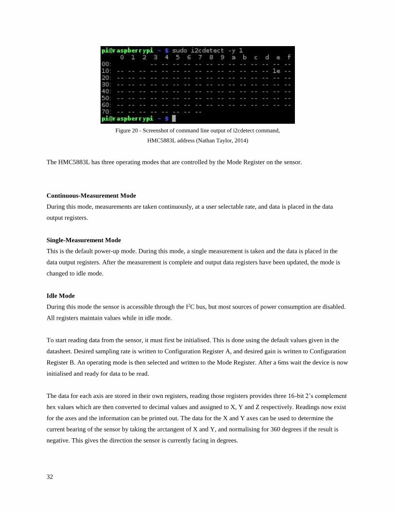
As the sensor uses I2C, the I2Cdetect command can be used once all the pins have been connected to check if it is
being detected. After determining that the sensor is connected properly and has an I2C address, the program to
interface with it can be written.
Page 32
32
Figure 20 - Screenshot of command line output of i2cdetect command,
HMC5883L address (Nathan Taylor, 2014)
The HMC5883L has three operating modes that are controlled by the Mode Register on the sensor.
Continuous-Measurement Mode
During this mode, measurements are taken continuously, at a user selectable rate, and data is placed in the data
output registers.
Single-Measurement Mode
This is the default power-up mode. During this mode, a single measurement is taken and the data is placed in the
data output registers. After the measurement is complete and output data registers have been updated, the mode is
changed to idle mode.
Idle Mode
During this mode the sensor is accessible through the I2C bus, but most sources of power consumption are disabled.
All registers maintain values while in idle mode.
To start reading data from the sensor, it must first be initialised. This is done using the default values given in the
datasheet. Desired sampling rate is written to Configuration Register A, and desired gain is written to Configuration
Register B. An operating mode is then selected and written to the Mode Register. After a 6ms wait the device is now
initialised and ready for data to be read.
The data for each axis are stored in their own registers, reading those registers provides three 16-bit 2’s complement
hex values which are then converted to decimal values and assigned to X, Y and Z respectively. Readings now exist
for the axes and the information can be printed out. The data for the X and Y axes can be used to determine the
current bearing of the sensor by taking the arctangent of X and Y, and normalising for 360 degrees if the result is
negative. This gives the direction the sensor is currently facing in degrees.
Page 33
33
TGS 2600 Module - General air quality
The TGS 2600 is a general air quality sensor, it is highly sensitive to low concentrations of gaseous air
contaminants. It has a detection range of 1 ~ 30 ppm of H2 and provides a reading that indicates the level of
contaminants present. The TGS 2600 is an analogue sensor, and so an ADC is used to convert the data from the
sensor into a usable form. It has four pins, the standard VIN and GND, as well as a data pin and a VIN for the
integrated heater. The VIN for both the sensor and the heater both connect to the 5V power rail. Power is applied to
the integrated heater in order to maintain the sensing element at a specific temperature which is optimal for sensing.
The data pin connects to the ADC in series with a resistor, as per the datasheet, to allow measurement of voltage.
Figure 21 – TGS 2600 wiring (Nathan Taylor, 2014)
The analogue-to-digital converter that is used is made specifically for the Raspberry Pi as an expansion board that
fits on top of the GPIO header pins. The ADC communicates with the Raspberry Pi via the I2C bus.
Page 34
34
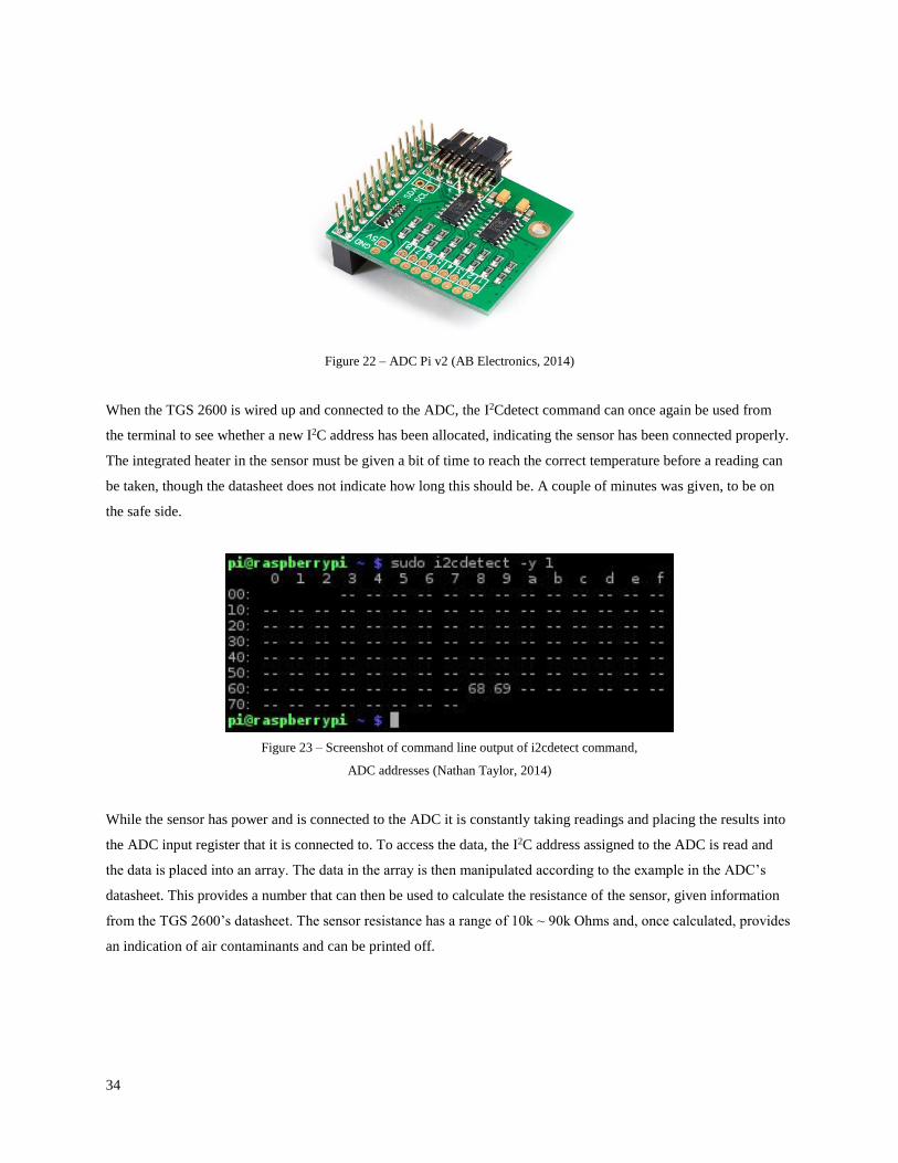
Figure 22 – ADC Pi v2 (AB Electronics, 2014)
When the TGS 2600 is wired up and connected to the ADC, the I2Cdetect command can once again be used from
the terminal to see whether a new I2C address has been allocated, indicating the sensor has been connected properly.
The integrated heater in the sensor must be given a bit of time to reach the correct temperature before a reading can
be taken, though the datasheet does not indicate how long this should be. A couple of minutes was given, to be on
the safe side.
Figure 23 – Screenshot of command line output of i2cdetect command,
ADC addresses (Nathan Taylor, 2014)
While the sensor has power and is connected to the ADC it is constantly taking readings and placing the results into
the ADC input register that it is connected to. To access the data, the I2C address assigned to the ADC is read and
the data is placed into an array. The data in the array is then manipulated according to the example in the ADC’s
datasheet. This provides a number that can then be used to calculate the resistance of the sensor, given information
from the TGS 2600’s datasheet. The sensor resistance has a range of 10k ~ 90k Ohms and, once calculated, provides
an indication of air contaminants and can be printed off.
Page 35
35
Anemometer Module
In the project design it was decided that the ability to measure wind speed should be included. Off-the-shelf
anemometers that could be made to interface easily with the Raspberry Pi were not readily available. While there
were models available, the cheap anemometers would have been too difficult to hack and modify, and the models
designed to be interfaced with other hardware were far too expensive. The decision was made that the anemometer
module would be a custom built sensor.
The design for the anemometer is basically a rotor, consisting of three cups connected horizontally to a central axle,
which rotates when driven by the wind. By measuring the speed that the axle is rotating, the wind speed can be
deduced, in a more or less empirical manner. The difficulty is in measuring the speed of the rotating axle. The way
that this was decided to be done was optically: attached to the axle is a perforated disc, and located above and below
the disk are an LED and a phototransistor.
Figure 24 – Optical anemometer design
As the axle rotates, and the disc with it, the phototransistor is illuminated by the LED each time the perforations
pass. The conductive state of the phototransistor can be measured and recorded, providing a way to estimate the
rotation speed of the axle in the form of a pulse counter.
A basic prototype version of the anemometer was constructed to test the design given above, using a 9mm wooden
dowel as the central axle, the hemispherical cups from a replacement part for a Maplin’s weather station, a
perforated cardboard disc, and a LED/phototransistor pair. The prototype was good enough to prove that the design
worked and that readings could be reliably taken, however, it proved to not be sturdy enough for real world
conditions. Unfortunately there was not enough time to build a sturdier prototype, more suitable outdoor use.
Page 36
36
Wind Vane Module
Being able to tell what direction the wind is blowing from is a feature of many weather stations, and so a wind vane
was added to the design for the project.
Wind direction is not a feature present on most of the commercial weather stations that you can buy, off-the-shelf
sensors or parts do not seem to be available. Because of this, and the anemometer module, it was decided that the
wind vane would be custom built also. Most modern instruments combine the directional wind vane with the
anemometer, allowing both instruments to use the same axis and provide coordinated readouts. While this may have
been more elegant, due to the complexity and the fact that the wind vane and the anemometer for the project are
different modules, they were built separately.
The design idea behind the wind vane is very similar to that of the anemometer, a horizontal arrow that is mounted
on an axle which is able to rotate freely. The arrow’s shape is designed so that it catches the wind and, because of
the axle, moves into the wind’s eye, indicating the direction from which the wind is blowing. To determine the
actual direction of the wind the absolute position of the axle on which the arrow is mounted must be determined.
As with the anemometer, an optical method was decided on for measuring the position of the axle. Two different
ways to implement this were tested. The first is, again, very similar to the anemometer and involves attaching a
perforated disk to the axle which rotates along with it. Located above the disk are LEDs and below are
phototransistors, or vice versa. Each time a phototransistor encounters a lit LED through a perforation the
phototransistor becomes conductive, a state that can be detected and recorded.
Figure 25 – Optical wind vane design
Page 37
37
The second implementation also involves LEDs and phototransistors, but instead of a disk mounted to the axle it
uses reflective material attached to the axle itself. The light from the LEDs reflects off of the material and the
phototransistor reacts. If there is no reflective material, then the phototransistor does not react.
A method is needed for both implementations so that they can recognise individual states that can be attributed to a
position, or direction. To do this a binary numeral system is used called reflected binary code. Also known as Gray
code, this system has the very useful feature that generated codes differ by only one bit from one position to another,
this limits the risks of reading errors for intermediary positions on both systems. The resolution that can be achieved
depends on the number of bits in the code, which is limited by the number of phototransistors that can be used.
For the second implementation a standard Gray code could be used, with a minimum resolution of 3-bits for reasons
of accuracy, and a maximum resolution of 5-bits because of the limited inputs available on the Raspberry Pi. A Gray
code of 3-bits gave the ability to recognise the cardinal and intercardinal directions: north, northeast, east, southeast,
south, southwest, west and northwest. A Gray code of 5-bits provides a precision of 11~12°. Both of which are
viable for determining wind direction.
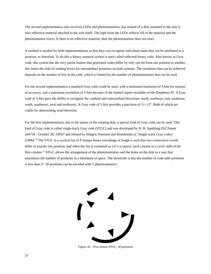
For the first implementation, due to the nature of the rotating disk, a special kind of Gray code can be used. This
kind of Gray code is called single-track Gray code (STGC) and was developed by N. B. Spedding (NZ Patent
264738 - October 28, 1994)9 and refined by Hiltgen, Paterson and Brandestini in "Single-track Gray codes"
(1996).10 The STGC is a cyclical list of P unique binary encodings of length n such that two consecutive words
differ in exactly one position, and when the list is examined as a P x n matrix, each column is a cyclic shift of the
first column.11 STGC allows the arrangement of the phototransistors and the holes on the disk in a way that
maximises the number of positions in a minimum of space. The downside is that the number of code-able positions
is less than 2n, 30 positions can be encoded with 5 phototransistors.
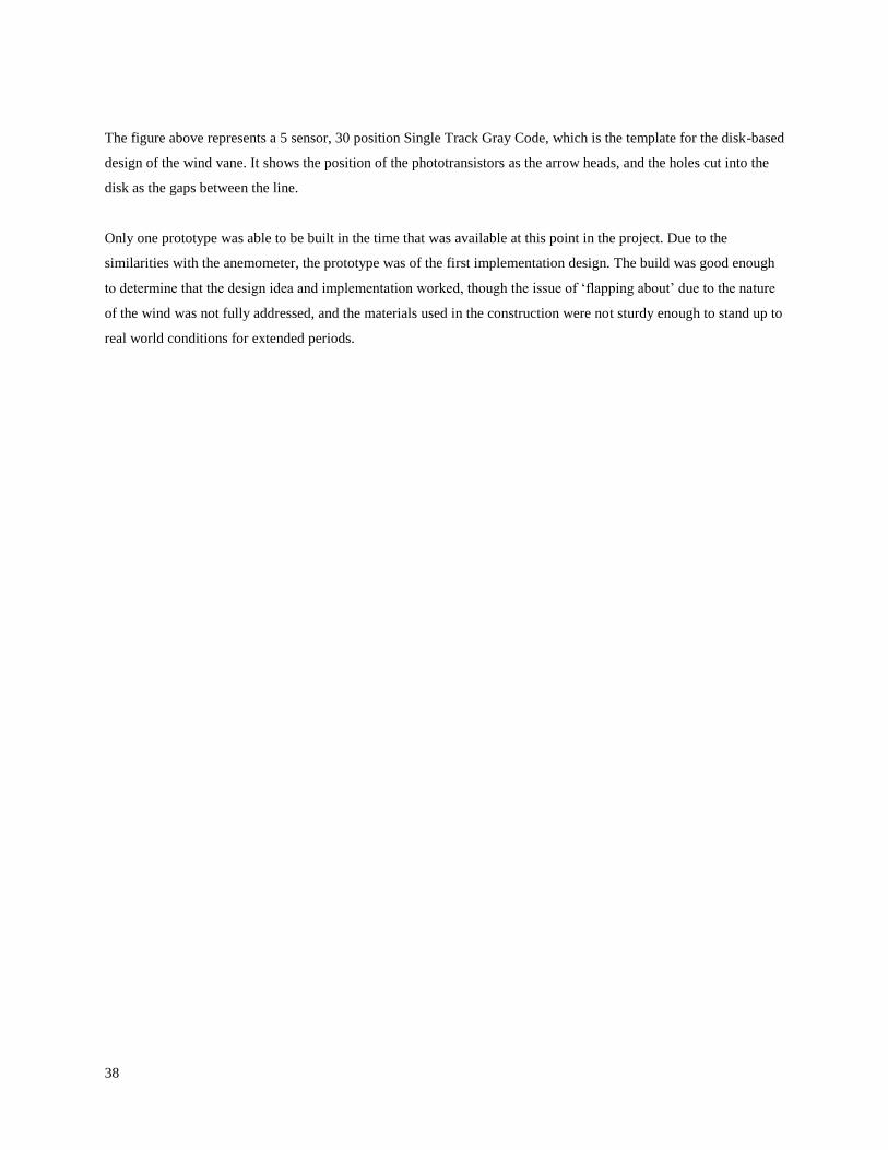
Figure 26 – Five sensor STGC, 30 positions
Page 38
38
The figure above represents a 5 sensor, 30 position Single Track Gray Code, which is the template for the disk-based
design of the wind vane. It shows the position of the phototransistors as the arrow heads, and the holes cut into the
disk as the gaps between the line.
Only one prototype was able to be built in the time that was available at this point in the project. Due to the
similarities with the anemometer, the prototype was of the first implementation design. The build was good enough
to determine that the design idea and implementation worked, though the issue of ‘flapping about’ due to the nature
of the wind was not fully addressed, and the materials used in the construction were not sturdy enough to stand up to
real world conditions for extended periods.
Page 39
39
IV. Evaluation and Results
This section of the report covers the calibration that was needed by some of the sensors, the results of the project
once all the modules had been completed, and the output of those results in a meaningful manner.
Calibration
Most of the sensors had been factory calibrated, with only a couple requiring some kind of manual calibration.
BMP085
The BMP085 sensor gave uncompensated readings for temperature and air pressure. To convert the data into °C and
hPa the readings had to be compensated using the formulas given in the data sheet. The calibration data used in the
formulas is specific to each individual sensor, thankfully that calibration data is provided and stored in EEPROM on
the sensor itself. This meant that the only difficulty lay in turning the temperature and air pressure compensation
formula into working code.
Figure 27 – BMP085 compensation formulas
Page 40
40
TGS 2600
TGS 2600 measures the concentrations of contaminants in the air. The output of this sensor is a measure of the
sensor’s resistance, which indicates the level of contaminants. The calibration of this sensor was less calibration and
more about presenting the data in a more understandable fashion. The sensor has a detection range of 1 ~ 30 ppm,
and a resistance range of 10k ~ 90k Ohms. Since there is no information in the datasheet regarding contaminant
levels relative to sensor resistance, estimates have to be made given the information that is available. This means
that, roughly speaking, a reading of 10k Ohms indicates air contaminants of 1 ppm, and a reading of 90k Ohms
indicates air contaminants of 30 ppm. From this it can be extrapolated that every 2,700~2,800 change in sensor
resistance indicates a rise or fall in contaminant levels by 1 ppm, that is every 1 ppm equals ~2,758 sensor
resistance. This gives more meaning to the standard sensor resistance reading that the sensor outputs.
HMC5883L
The HMC5883L is the digital compass module that the project uses to orientate its direction. The program written
for the sensor outputs a bearing between 0-360°, with 0° indicating north. When first testing the sensor, it was
noticed that the readings were not quite right. The testing was done by physically rotating the device through four
90° steps, taking a reading at each step. This showed that the readings were out, though not by very much.
The program was modified to take continuous readings for a set amount of time and to output the readings to a file.
Then, while the program was running the device was rotated backwards and forwards through 360°. The data in the
file was used to create a plot, which showed that the readings were slightly off.
Page 41
41
Figure 28 – Scatter plot of raw compass data (Nathan Taylor, 2014)
The program was modified once again to calculate the standard offset that should be applied to correct the readings.
Using the same procedure, the program was run again and the device was rotated through 360°, when finished it
printed off the offsets that needed to be applied to the calculations.
The first program was then modified to take the offsets into account, and the initial test of four 90° steps re-run to
verify that the readings were now more accurate.
Page 42
42
Anemometer
As one of the custom built sensors, the anemometer module requires some calibration. It is able to record how many
pulses occur over a set period of time or how long it takes to record a set number of pulses. The difficulty lies in
relating one of these measures to the speed of the wind. While it is entirely possible to compute this mathematically,
a more practical approach was suggested online and as it sounded far more fun it was decided to take it.
The anemometer was attached to a broom handle, the Raspberry Pi and associated parts were bundled up and a trip
was taken by car. Not many readings needed to be taken to get a basic idea of the relation between revolutions of the
anemometer and the current speed. Readings were taken at different intervals and a constant speed was maintained
while the readings were being taken. Readings for each speed were taken in both directions on the route that was
followed to take the influence of the wind into account as much as possible, and the mean of the two sets of readings
was used. It was found that for low speeds the relation was around 1.8-2.0 pulses per 1 Mph. This was for speeds of
30 Mph and lower, above this the anemometer started to become unstable and the experiment was swiftly stopped.
Sensor Output
A weather station provides information on the current atmospheric conditions, and so the data collected by the
sensors has to be output in some way so that it may be useful. The project does this through the use of a central
Python program that calls the classes for the sensors, records and collates the data, and then outputs it to the
command line.
Figure 29 – Command line output of sensor readings (Nathan Taylor, 2014)
Page 43
43
The command line was chosen as the initial location for the output as it is simple, quick and useful for debugging.
However, presentation of results matters and as one of the goals of the project is its potential as a teaching tool there
was further opportunity to create an ‘Output Module’.
Weather stations also tend to be located outside and while there is the option of logging in remotely and reading the
data from the command line, why not utilise the Raspberry Pi further and also turn it into a webserver. The data
from the sensors could then be output to a webpage and could be checked from anywhere with an internet
connection.
The next challenge was how to take the data from the Python program that was running the sensors and interface it
with an HTML file. This was accomplished using a microframework for Python, called Flask. Flask is a lightweight
web application framework which uses the Werkzeug Web Server Gateway Interface (WSGI) toolkit and the Jinja2
template engine. It is called a microframework because it keeps the core simple but extensible, it does not have any
components where third-party libraries already exist that provide common functionality. It does, however, support
extensions that can add such functionality.
Flask is very useful as it allows the dynamic creation of HTML content through the use of templates. Using
templates allows a basic layout for the webpages to be set and also provides the ability to define the dynamic
elements. This means that variables from the Python program that Flask is included in, such as the data from the
weather station, can be inserted into and used on the webpage. It also means that when the webpage is refreshed,
new readings are taken from the sensors and the data on the page is also updated.
Page 45
45
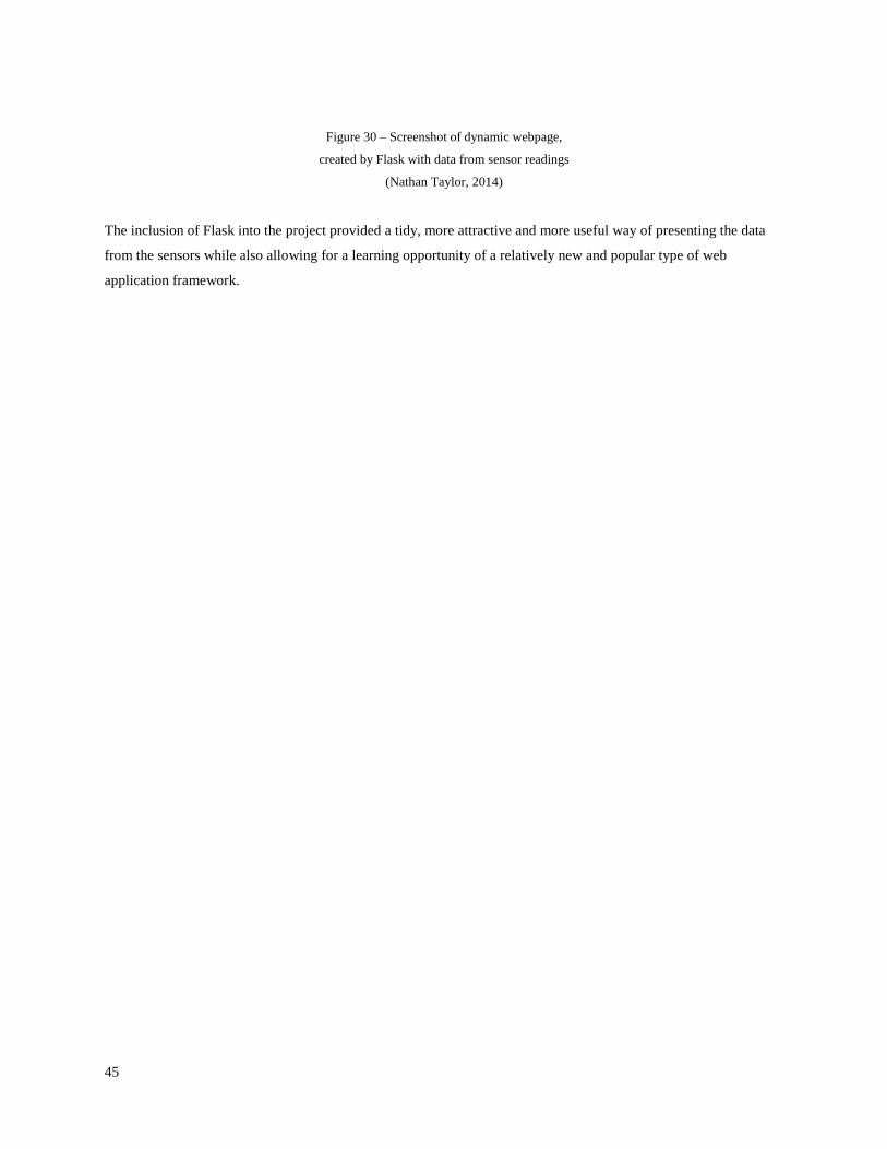
Figure 30 – Screenshot of dynamic webpage,
created by Flask with data from sensor readings
(Nathan Taylor, 2014)
The inclusion of Flask into the project provided a tidy, more attractive and more useful way of presenting the data
from the sensors while also allowing for a learning opportunity of a relatively new and popular type of web
application framework.
Page 46
46
V. Conclusion (1,500)
This section of the report aims to summarise what was accomplished during the project, present any findings that
were made and look at the final product. It also covers what else could have been accomplished if there had been
more time, or that could be added in future expansions. The last part asks if the project achieved what it set out to at
the beginning.
Summary
Starting with nothing but the Raspberry Pi and design ideas, the needed hardware for the base platform was
acquired. The research into the availability and capability of sensors conducted, and four off-the-shelf sensors were
ordered. Work then started on integrating the sensors with the Raspberry Pi and writing programs to interface with
them. At the same time materials for the custom built sensors were ordered, and work on their design was started.
Being the main focus of the project, as expected, these tasks took up the majority of development time and were not
without their problems. Towards the end of the project time was spent on creating a more elegant and attractive
method for outputting the data from the sensor readings. When the time came to stop work on the project, what had
actually been accomplished?
The end result is that the project has eight completed modules, which consist of the base module, six sensor modules
and an output module. The project is able to take readings for temperature, air pressure, humidity, direction, air
quality, wind speed and wind direction, and output the data from these readings to a dynamically created webpage
that can be viewed from any capable device with an internet connection. The project, as it stands, accomplishes and
provides everything it set out to in the original design, but it is by no means finished or complete.
Page 47
47
Figure 31 – Raspberry Pi connected to breadboard with sensors wired in. (Nathan Taylor, 2014)
Page 48
48
Expansion
In terms of expanding the project, there were many options that were considered but ruled out due to time
constraints. Some of these are explored below.
Light levels
A feature that was considered for addition to the project was the ability to measure the relative level of light
intensity that the sensor was currently exposed to. The amount of light falling on a surface is defined as illuminance,
and is measured in lux. The measurement and perception of light can be an in-depth topic. The level of light in an
indoor area has a direct impact on the task being performed, being too bright or too dim could easily have a negative
impact. The brightness of the sky is often given using illuminance values measured on an unobstructed horizontal
plane. Those values represent the total illumination available from the sky, and can be used to determine the
condition outside using a light sensor.
Adding a light sensor to the project could be done simply by using a Light Dependent Resistor and building a table
of average values based on experiments under different conditions.
Alternatively, digital luminosity sensors exist that could be interfaced with the project. One such sensor is the
TSL2561, which contains both infrared and full spectrum diodes, allowing you to measure infrared, full-spectrum or
human-visible light. It can detect light ranges from 0.1 - 40,000+ lux. Deep twilight measures around 0.1 lux and
full daylight measures 10,752 lux.
Cloud detection
The identification and reporting of clouds contributes to the process of weather forecasting, they effect both daily
weather and Earth’s climate. As such, a method of cloud detection was another idea for the project.
The basic idea behind the module would be to utilise a webcam or camera module with the Raspberry Pi along with
time-lapse software to take pictures. The next step would be to use an external library, such as OpenCV (Open
Source Computer Vision), to analyse and compare the pictures and their histograms to determine a measure of
‘cloudiness’. This measure could then be compared with a current picture, and the determined ‘cloudiness’ provided
as an output.
Rain detection
While rain detection might not have many practical applications aside from being able to tell if it is raining, it is
another piece of information that the weather station could report on. There are a number of concepts that cover how
a rain detection sensor could be added to the project.
Page 49
49
These include the use of a moisture sensor for measuring the relative levels of moisture around the device, coupled
with a method detecting rain drops. This could be achieved through the use of a sound sensor, attaching it to a thin
sheet of aluminium or a similar material, then converting the output to a logic level and counting the pulses. The
level of noise from other sources could prove this to be completely ineffective, however, depending upon the
sensitivity of the sensor. An alternate method could be to substitute the sound sensor for a piezo vibration sensor,
again attaching it to a sheet of aluminium. The rain drops hitting the sheet should give an indication of the amount
and severity of rainfall. Both of these ideas could do well as ‘proof of concept’, but would need improving upon for
long term use.
Rain gauge
The measuring and reporting of rainfall is something that many true weather stations provide, as do some of the
more expensive commercial ones. Adding this capability to the project could be informative, useful and interesting.
This could be done through the addition of a rain gauge. A rain gauge counts the depth of rainfall per unit area. For
example, it might report that over the last 24 hour period there were 2mm of rainfall per metre squared. The borough
and city of Manchester is 115.6km2, over an area of that size 2mm of rainfall equates to around 231,000 cubic
metres or 92 Olympic-size swimming pools. The average rainfall for Manchester in April is 54mm.12 So, having a
rain gauge might be interesting.
There are several different types of rain gauge, but the most common is called a tipping bucket rain gauge. A
tipping bucket rain gauge consists of a funnel that collects and channels the precipitation into a small seesaw-like
container. After a pre-set amount of precipitation falls, the lever tips, dumping the collected water and sending an
electrical signal. The buckets are calibrated to a volume of water, counting the number of times the switch closes
indicates how much rainfall there has been.
This type of rain gauge is not as accurate as some of the others, as the rainfall may stop before the level has tipped.
When it next starts raining it may take no more than a couple of drops to tip the lever, which would then indicate the
pre-set amount has fallen when it has actually only been a fraction of that amount. The advantage of the tipping
bucket rain gauge is that the character of the rain can be easily obtained. Rainfall character is usually decided by the
total amount of rain that has fallen in a set period, say an hour. By counting the number of ‘clicks’ from the rain
gauge in a 10 minute period, it can be decided whether the rainfall is light, medium or heavy.
An implementation of this type of rain gauge is available from Maplins and can be hacked to interface with the
Raspberry Pi without much difficulty, as such it will be the focus of this hypothetical sensor module. Each tip of the
bucket passes a magnet over a reed switch, making a momentary electrical connection, which is identical to a button
press. This means that the sensor can be connected to a GPIO pin, and the relatively recent inclusion of GPIO
Page 50
50
interrupts can be used to monitor it. Each time the circuit is closed by the bucket tipping, a software event is
triggered which makes it easy to create a monitoring program.
Critique
The purpose of Raspberry Pi Projects for Schools was to develop a project that could be utilised as a teaching and
learning tool for and by school children. A project that could enthuse those school children to take a greater interest
in Computer Science, and to show them it is not just about creating spreadsheets and word documents, and
designing webpages.
A list of requirements was made that the project should try to fulfil, such as the modular design and interdisciplinary
nature. A design was drawn up, and it was decided that the project would entail the building of a weather station. A
list of potential modules for the weather station was made, which was then shortened to a more realistic number.
Development work was then started on the project. The work progressed relatively smoothly, with any difficulties
encountered overcome without too much additional time spent on them.
When the time came for development work to stop, the project was in good shape. All the modules set out in the
design had been completed and worked, though the custom built sensors were more ‘proof of concept’ than ‘finished
model’. An additional module that dealt with the output from the other modules had been added and completed,
providing a more polished presentation of the data. The modular and interdisciplinary requirements had been met.
The current state of the project, however, does not lend itself as a teaching tool nor is it as complete as would be
liked. The software driving the project is a working design rather than a polished, finished product and requires
some revision. Not much can be done with the hardware, without manufacturing of custom PCBs and an proper
enclosure, but including the ability for outside use is something that would have been good to include. Likewise,
construction of sturdier versions of the custom sensors was a goal that was in the works when time ran out.
Despite the shortcomings, the project did meet the majority of the original requirements, it includes all of the
modules it intended to and produces a useful, readable output. The project could be used as a tool for teaching and
learning, and it is the hope that it would interest and enthuse more people towards Computer Science. Did it achieve
what it set out to in the beginning? The belief is that yes it did, and that it could be a good teaching tool, but with a
little more work it has the potential to be a great teaching tool.
Page 51
51
VI. References
[1] Kershaw, A. (2012). Michael Gove brands ICT curriculum 'a mess'. Available:
http://www.independent.co.uk/news/education/education-news/michael-gove-brands-ict-curriculum-a-mess-
6287885.html.
[2] Department for Education. (2012). ‘Harmful’ ICT curriculum set to be dropped to make way for rigorous
computer science. Available: https://www.gov.uk/government/news/harmful-ict-curriculum-set-to-be-dropped-to-
make-way-for-rigorous-computer-science.
[3] Raspberry Pi Foundation. (2012). Raspithon. Available: http://www.raspberrypi.org/tag/raspithon/.
[4] Manchster Raspberry Jam. (2014). Bring your Raspberry Pi to life... Available: http://mcrraspjam.org.uk/about/.
[5] ScratchMyPi. (2014). Delivering the primary computing curriculum. Available:
http://www.scratchmypi.co.uk/school-workshops/.
[6] Raspberry Jam. (2014). What is #RaspberryJam?. Available: http://raspberryjam.org.uk/what-is-raspberryjam/.
[7] NXP Semiconductors. (2014). UM10204 - I2C-bus specification and user manual. Available:
http://www.nxp.com/documents/user_manual/UM10204.pdf.
[8] Renesas. (2003). Serial Peripheral Interface and Inter-IC. Available:
http://documentation.renesas.com/doc/products/region/rtas/mpumcu/apn/spi_I2C.pdf.
[9] Spedding, Norman Bruce. (1994) A position encoder: A method of creating a single track absolute position
rotary or linear encoder of varying resolutions using equi-spaced detectors. Available:
http://www.winzurf.co.nz/Single_Track_Grey_Code_Patent/Single_track_Grey_code_encoder_patent.pdf
[10] Hiltgen, Alain P.; Kenneth G. Paterson; Marco Brandestini (1996). "Single-Track Gray Codes" (PDF). IEEE
Transactions on Information Theory 42 (5): 1555–1561.doi:10.1109/18.532900.
[11] Etzion, Tuvi; Moshe Schwartz (1999). "The Structure of Single-Track Gray Codes" (PDF). IEEE Transactions
on Information Theory 45 (7): 2383–2396.doi:10.1109/18.796379.
[12] Met Office. (2012). Manchester Airport 1981 – 2010 averages. Available:
http://www.metoffice.gov.uk/climate/uk/averages/19812010/sites/manchester_airport.html
Page 52
52
VII. Figures
1. Amazon UK. (2014). Technoline WS-9130 Digital Weather Station. Digital image, available:
http://www.amazon.co.uk/Technoline-WS-9130--Digital-Weather-
Controlled/dp/B002DNE0IK/ref=sr_1_5?s=outdoors&ie=UTF8&qid=1398516504&sr=1-5.
2. Maplins. (2014). Silver USB Wireless Touchscreen Weather Forecaster. Digital image, available:
http://www.maplin.co.uk/p/silver-usb-wireless-touchscreen-weather-forecaster-n96fy.
3. Wikipedia. (2014). I2C Data transfer sequence, timing diagram. Digital image, available:
http://upload.wikimedia.org/wikipedia/commons/6/64/I2C_data_transfer.svg.
4. Wikipedia. (2014). SPI data transmission diagram. Digital image, available:
http://upload.wikimedia.org/wikipedia/commons/b/bb/SPI_8-bit_circular_transfer.svg.
5. Wikipedia. (2014). SPI timing diagram showing clock polarity and phase. Digital image, available:
http://upload.wikimedia.org/wikipedia/commons/6/6b/SPI_timing_diagram2.svg.
6. Taylor, N. (2014). Assorted components for project’s base module. Digital image.
7. Adafruit. (2014). BMP085 pressure and temperature sensor. Digital image, available:
https://www.adafruit.com/images/970x728/391-00.jpg.
8. Adafruit. (2014). DHT22 temperature and humidity sensor. Digital image, available:
https://www.adafruit.com/images/970x728/385-00.jpg.
9. RS Components and Allied Electronics. (2014.) TGS2600 General air quality sensor. Digital image, available:
http://img-europe.electrocomponents.com/largeimages/R538996-01.jpg.
10. Adafruit. (2014). HMC5883L 3-Axis digital compass. Digital image, available:
http://www.adafruit.com/images/970x728/1746-00.jpg.
11. Wikipedia. (2014). Hemispherical cup anemometer invented in 1846 by John Robinson. Digital image, available:
http://upload.wikimedia.org/wikipedia/commons/6/61/Wea00920.jpg.
12. APRS World. (2014). Modern wind vane. Digital image, available: http://www.aprsworld.com/albums/Wind-
Vane/Wind_Vane_b.sized.jpg.
13. Taylor, N. (2014). Adafruit Pi Cobbler. Digital image.
14. Taylor, N. (2014). Raspberry Pi connected to a breadboard via Pi Cobbler. Digital image.
15. Taylor, N. (2014). LEDs connected to 3v3 rail of the Raspberry Pi. Digital image.
16. Taylor, N. (2014). DHT22 sensor wired into a breadboard. Digital image.
17. Taylor, N. (2014). BMP085 sensor wired into a breadboard. Digital image.
18. Taylor, N. (2014). Screenshot of i2cdetect output with BMP085 connected. Digital image.
19. Taylor, N. (2014). HMC5883L sensor wired into a breadboard. Digital image.
20. Taylor, N. (2014). Screenshot of i2cdetect output with HMC5883L connected. Digital image.
21. Taylor, N. (2014). TGS 2600 sensor wired into a breadboard. Digital image.
22. AB Electronics. (2014). ADC Pi v2. Digital image, available:
http://www.abelectronics.co.uk/docs/stock/raspberrypi/adcpi2/adcpiV2_1.jpg.
23. Taylor, N. (2014). Screenshot of i2cdetect output with TGS2600 and ADC connected. Digital image.
Page 53
53
24. Yoctopuce. (2013). Optical anemometer design. Digital image, available: http://www.yoctopuce.com/EN/.
25. Yoctopuce. (2013). Optical wind vane design. Digital image, available: http://www.yoctopuce.com/EN/.
26. Wikipedia. (2014). Reference design for 5 sensor, 30 position Single Track Gray Code rotary encoder. Digital
image, available: http://upload.wikimedia.org/wikipedia/commons/5/5e/Enkelspoors-Graycode.svg.
27. Taylor, N. (2014). Screenshot of BMP085 compensation formulas from datasheet. Digital image.
28. Taylor, N. (2014). Scatter plot of raw compass data from HMC5883L calibration. Digital image.
29. Taylor, N. (2014). Command line output of project sensor readings. Digital image.
30. Taylor, N. (2014). Dynamic webpage output of project sensor readings. Digital image.
31. Taylor, N. (2014). Raspberry Pi connected to breadboard with all sensors wired up. Digital image.