ChaDter 13 Rate Distortion Theory The description of an arbitrary real number requires an infinite number of bits, so a finite representation of a continuous random variable can never be perfect. How well can we do? To frame the question appropriately, it is necessary to define the “goodness” of a representation of a source. This is accomplished by defining a distortion measure which is a measure of distance between the random variable and its representation. The basic problem in rate distortion theory can then be stated as follows: given a source distribution and a distortion measure, what is the minimum expected distortion achievable at a particular rate? Or, equivalently, what is the minimum rate description required to achieve a particular distortion? One of the most intriguing aspects of this theory is that joint descriptions are more efficient than individual descriptions. It is simpler to describe an elephant and a chicken with one description than to describe each alone. This is true even for independent random variables. It is simpler to describe X1 and X2 together (at a given distortion for each) than to describe each by itself. Why don’t independent problems have independent solutions? The answer is found in the geometry. Apparently rectangular grid points (arising from independent descrip- tions) do not fill up the space efficiently. Rate distortion theory can be applied to both discrete and continuous random variables. The zero-error data compression theory of Chapter 5 is an important special case of rate distortion theory applied to a discrete source with zero distortion. We will begin by considering the simple problem of representing a single continuous random variable by a finite number of bits. 336 Elements of Information Theory Thomas M. Cover, Joy A. Thomas Copyright 1991 John Wiley & Sons, Inc. Print ISBN 0-471-06259-6 Online ISBN 0-471-20061-1
Transcript
ChaDter 13
Rate Distortion Theory
The description of an arbitrary real number requires an infinite number of bits, so a finite representation of a continuous random variable can never be perfect. How well can we do? To frame the question appropriately, it is necessary to define the “goodness” of a representation of a source. This is accomplished by defining a distortion measure which is a measure of distance between the random variable and its representation. The basic problem in rate distortion theory can then be stated as follows: given a source distribution and a distortion measure, what is the minimum expected distortion achievable at a particular rate? Or, equivalently, what is the minimum rate description required to achieve a particular distortion?
One of the most intriguing aspects of this theory is that joint descriptions are more efficient than individual descriptions. It is simpler to describe an elephant and a chicken with one description than to describe each alone. This is true even for independent random variables. It is simpler to describe X1 and X2 together (at a given distortion for each) than to describe each by itself. Why don’t independent problems have independent solutions? The answer is found in the geometry. Apparently rectangular grid points (arising from independent descrip- tions) do not fill up the space efficiently.
Rate distortion theory can be applied to both discrete and continuous random variables. The zero-error data compression theory of Chapter 5 is an important special case of rate distortion theory applied to a discrete source with zero distortion.
We will begin by considering the simple problem of representing a single continuous random variable by a finite number of bits.
336
Elements of Information TheoryThomas M. Cover, Joy A. Thomas
Copyright 1991 John Wiley & Sons, Inc.Print ISBN 0-471-06259-6 Online ISBN 0-471-20061-1
13.1 QUANTIZATION 337
13.1 QUANTIZATION
This section on quantization motivates the elegant theory of rate distor- tion by showing how complicated it is to solve the quantization problem exactly for a single random variable.
Since a continuous random source requires infinite precision to repre- sent exactly, we cannot reproduce it exactly using a finite rate code. The question is then to find the best possible representation for any given data rate.
We first consider the problem of representing a single sample from the source. Let the random variable to be represented be X and let the representation of X be denoted as X(X). If we are given R bits to represent X, then the function X can take on 2R values. The problem is to find the optimum set of values for X (called the reproduction points or codepoints) and the regions that are associated with each value X.
For example, let X - NO, (T’), and assume a square-d error distortion measure. In this case, we wish to find the function X(X) such that X takes on at most 2R values and minimizes E(X - X(XN2. If we are given 1 bit to represent X, it is clear that the bit should distinguish whether X > 0 or not. To minimize squared error, each reproduced symbol should be at the conditional mean of its region. This is illustrated in Figure 13.1. Thus
ifxr0, (13.1) - I d %, ifx<O.
n-
0.4
0.35
0.3
0.25
2 0.2
0.15
-0.7979 0.7979
Figure 13.1. One bit quantization of a Gaussian random variable.
338 RATE DlSTORTlON THEORY
If we are given 2 bits to represent the sample, the situation is not as simple. Clearly, we want to divide the real line into four regions and use a point within each region to represent the sample. But it is no longer immediately obvious what the representation regions and the recon- struction points should be.
We can however state two simple properties of optimal regions and reconstruction points for the quantization of a single random variable:
l Given a set of reconstruction points, the distortion is minimized by mapping a source random variable X to the representation X(w) that is closest to it. The set of regions of %’ defined by this mapping is called a Voronoi or Dirichlet partition defined by the reconstruc- tion points.
l The reconstruction points should minimize the conditional expected distortion over their respective assignment regions.
These two properties enable us to construct a simple algorithm to find a “good” quantizer: we start with a set of reconstruction points, find the optimal set of reconstruction regions (which are the nearest neighbor regions with respect to the distortion measure), then find the optimal reconstruction points for these regions (the centroids of these regions if the distortion is squared error), and then repeat the iteration for this new set of reconstruction points. The expected distortion is decreased at each stage in the algorithm, so the algorithm will converge to a local minimum of the distortion. This algorithm is called the Lloyd algorithm [ 1811 (for real-valued random variables) or the generaked Lloyd aZ- gorithm [80] (for vector-valued random variables) and is frequently used to design quantization systems.
Instead of quantizing a single random variable, let us assume that we are given a set of n i.i.d. random variables drawn according to a Gaussian distribution. These random variables are to be represented using nR bits. Since the source is i.i.d., the symbols are independent, and it may appear that the representation of each element is an independent problem to be treated separately. But this is not true, as the results on rate distortion theory will show. We will represent the entire sequence by a single index taking ZnR values. This treatment of entire sequences at once achieves a lower distortion for the same rate than independent quantization of the individual samples.
13.2 DEFINITIONS
Assume that we have a source that produces asequenceX,,X,,...,X, i.i.d. -p(x), x E 35 We will assume that the alphabet is finite for the
13.2 DEFlNlTlONS 339
proofs in this chapter; but most of the proofs can be extended to continuous random variables.
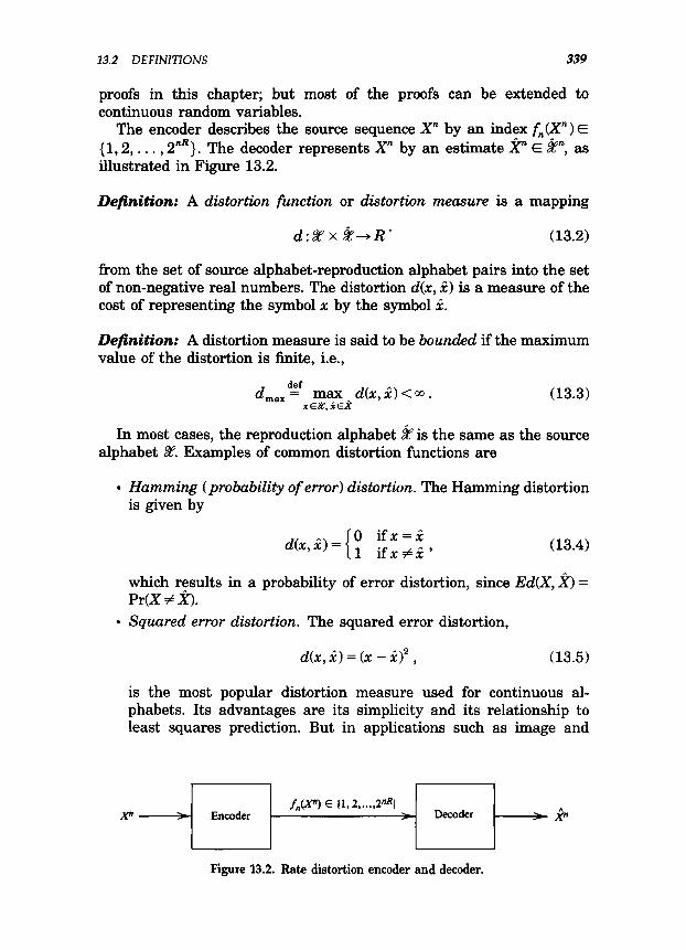
The encoder describes the source sequence X” by an index f,(X”> E {1,2,. . . , ZnR}. The decoder represents X” by an estimate p E @, as illustrated in Figure 13.2.
Definition: A distortion function or distortion measure is a mapping
d:%‘x&-R+ (13.2)
from the set of source alphabet-reproduction alphabet pairs into the set of non-negative real numbers. The distortion d(x, i) is a measure of the cost of representing the symbol x by the symbol i.
Definition: A distortion measure is said to be bounded if the maximum value of the distortion is finite, i.e.,
d def
max = max d(x,i)<m. XEBe”, i&t
(13.3)
In most cases, the reproduction alphabet k is the same as the source alphabet %‘. Examples of common distortion functions are
l Hamming (probability of error) distortion. The Hamming distortion is given by
d&i) = 0 ifx=i 1 ifx#? (13.4)
which results in a probability of error distortion, since Ed(X, @ = Pr(X #X).
l Squared error distortion. The squared error distortion,
d(x, i) = (3~ - i>2 , (13.5)
is the most popular distortion measure used for continuous al- phabets. Its advantages are its simplicity and its relationship to least squares prediction. But in applications such as image and
fnw9 E (1,2,...Pl P > Encoder > Decoder ,‘- &
Figure 13.2. Rate distortion encoder and decoder.
340 RATE DlSTORTlON THEORY
speech coding, various authors have pointed out that the mean squared error is not an appropriate measure of distortion as ob- served by a human observer. For example, there is a large squared error distortion between a speech waveform and another version of the same waveform slightly shifted in time, even though both would sound very similar to a human observer.
Many alternatives have been proposed; a popular measure of distor- tion in speech coding is the Itakura-Saito distance, which is the relative entropy between multivariate normal processes. In image coding, how- ever, there is at present no real alternative to using the mean squared error as the distortion measure.
The distortion measure is defined on a symbol-by-symbol basis. We extend the definition to sequences by using the following definition:
Definition: The distortion between sequences xn and in is defined by
d(x”,P) = ; $ d(xi, &) . 11
(13.6)
So the distortion for a sequence is the average of i;he per symbol distortion of the elements of the sequence. This is not the only reason- able definition. For example, one may want to measure distortion between two sequences by the maximum of the per symbol distortions. The theory derived below does not apply directly to this case.
Definition: A (2nR, n) rate distortion code consists of an encoding function,
f, : Z”+ {1,2,. . . , 2nR} , (13.7)
and a decoding (reproduction) function,
g,:{1,2 ,..., znR}+P.
The distortion associated with the (2nR, n) code is defined as
D = Ed(X”, g,( f, (x” 1)) 3
(13.8)
(13.9)
where the expectation is with respect to the probability distribution on X, i.e.,
D = c p(x”) dtx”, g,( f,b” ))) . xn
(13.10)
13.2 DEFiNITIONS 341
The set of n-tuples g,(l), g,(2), . . . , g,(2’?, denoted bY e(l), . l -3 p~2”~), constitutes the codebook, and f,‘(l), . . . , f,‘<2’? are the associated assignment regions.
Many terms are used to describe the replacement of X” by its quantized version p(w). It is common to refer to * as the vector quantization, reproduction, reconstruction, representation, source code, or estimate of X”.
Definition: A rate distortion pair (R, D) is said to be achievable if there exists a sequence of (2”R, n) rate distortion codes ( f,, g, 1 with lim,,, E&X”, g,( fn,cx” ))I 5 D.
Definition: The rate distortion region for a source is the closure of the set of achievable rate distortion pairs (R, D).
Definition: The rate distortion function R(D) is the infimum of rates R such that (R, D) is in the rate distortion region of the source for a given distortion D.
Definition: The distortion rate function D(R) is the inflmum of all distortions D such that (R, D) is in the rate distortion region of the source for a given rate R.
The distortion rate function defines another way of looking at the boundary of the rate distortion region, which is the set of achievable rate distortion pairs. We will in general use the rate distortion function rather than the distortion rate function to describe this boundary, though the two approaches are equivalent.
We now define a mathematical function of the source, which we call the information rate distortion function. The main result of this chapter is the proof that the information rate distortion function is equal to the rate distortion function defined above, i.e., it is the infimum of rates that achieve a particular distortion.
Definition: The information rate distortion function R"'(D) for a source X with distortion measure d(x, LC) is defined as
R"'(D) = p(ilx) :
min pWp(ilx)d(x,
I(X, 2) (13.11) i&D
where the minimization is over all conditional distributions p(i)x) for which the joint distribution p(x, i) = p(x)p(ilz) satisfies the expected distortion constraint.
342 RATE DlSTORTION THEORY
Paralleling the discussion of channel capacity in Chapter 8, we initially consider the properties of the information rate distortion func- tion and calculate it for some simple sources and distortion measures. Later we prove that we can actually achieve this function, i.e., there exist codes with rate R”‘(D) with distortion D. We also prove a converse establishing that R 1 R”‘(D) for any code that achieves distortion D.
The main theorem of rate distortion theory can now be stated as follows:
Theorem 13.2.1: The rate distortion function for an i.i.d. source X with distribution p(x) and bounded distortion function d(x, i) is equal to the associated information rate distortion function. Thus
This theorem shows that the operational definition of the rate distor- tion function is equal to the information definition. Hence we will use R(D) from now on to denote both definitions of the rate distortion function. Before coming to the proof of the theorem, we calculate the information rate distortion function for some simple sources and distor- tions.
13.3 CALCULATION OF THE RATE DISTORTION FUNCTION
13.3.1 Binary Source
We now find the description rate R(D) required to describe a Bernoulli(p) source with an expected proportion of errors less than or equal to D.
Theorem 13.3.1: The rate distortion function for a Bernoulli( p> source with Hamming distortion is given by
O~D~min{p,l-p}, D>min{p,l-p}. (13.13)
Proof: Consider a binary source X - Bernoulli(p) with a Hamming distortion measure. Without loss of generality, we may assume that p < fr . We wish to calculate the rate distortion function,
R(D) = min Icx;&. (13.14) p(ilr) : cc,, ij p(le)p(ilx)m, i)=D
Let 69 denote modulo 2 addition. Thus X$X = 1 is equivalent to X # X.
13.3 CALCULATlON OF THE RATE DlSTORTlON FUNCTION 343
We cannot minimize 1(X, X) directly; instead, we find a lower bound and then show that this lower bound is achievable. For any joint distribution satisfying the distortion constraint, we have
WC a = H(X) - H(X@) = H(p) - H(XcBX(2) (13.16)
H(p)-H(Xa32) (13.17)
IH(p)--H(D), (13.18)
since Pr(X #X) I D and H(D) increases with D for D 5 f . Thus
R(D)zH(p)-H(D). (13.19)
We will now show that the lower bound is actually the rate distortion function by finding a joint distribution that meets the distortion con- straint and has 1(X, X) = R(D). For 0 I D 5 p, we can achieve the value of the rate distortion function in (13.19) by choosing (X, X) to have the joint distribution given by the binary symmetric channel shown in Figure 13.3.
We choose the distribution of X at the input of the channel so that the output distribution of X is the specified distribution. Let r = Pr(X = 1). Then choose r so that
r(l-D)+(l-r)D=p, (13.20)
or
(13.21)
P-D 1-W
1-D 0
1 1-D
0 l-p
X
1 P
Figure 13.3. Joint distribution for binary source.
344 RATE DISTORTlON THEORY
I(x;~=HGX)-H(XI~=H(p)-H(D), (13.22)
and the expected distortion is RX # X) = D. If D 2 p, then we can-achieve R(D) = 0 by letting X = 0 with probabili-
ty 1. In this case, Z(X, X) = O-and D = p. Similarly, if D 2 1 - p, we cm achieve R(D I= 0 by setting X = 1 with probability 1.
Hence the rate distortion function for a binary source is
OrD= min{p,l-p}, D> min{p,l-p}. (13.23)
This function is illustrated in Figure 13.4. Cl
The above calculations may seem entirely unmotivated. Why should minimizing mutual information have anything to do with quantization? The answer to this question must wait until we prove Theorem 13.2.1.
13.3.2 Gaussian Source
Although Theorem 13.2.1 is proved only for discrete sources with a bounded distortion measure, it can also be proved for well-behaved continuous sources and unbounded distortion measures. Assuming this general theorem, we calculate the rate distortion function for a Gaus- sian source with squared error distortion:
Theorem 13.3.2: The rate distortion function for a N(0, u2) source with squared error distortion is
1 2 +%, OsDsg2,
(13.24) 0, D>U2.
I I I I 0 0.1 0.2 0.3 0.4 0.5 0.6 0.7 0.8 0.9
D
Figure 13.4. Rate distortion function for a binary source.
13.3 CALCULATZON OF THE RATE DlSTORTlON FUNCTION 345
proof= Let X be -N(O, a’). By the rate distortion theorem, we have
R(D) = min I(X, 2) . (13.25) flilx) : E(2-m2sD
As in the previous example, we first 6nd a lower bound for the rate distortion function and then prove that this is achievable. Since E(X - a2 5 D, we observe
Z(X, 2) = h(X) - h(X(X) (13.26)
1 = 2 log(27re)(r2 - h(X - XIX)
2 f log(27re)cr2 - h(X - X)
1 2 2 log(27re)02 - h(N(0, E(X - 2)“))
1 = 5 log(27re)(r2 - f log(2ne)E(X - X)”
(13.27)
(13.28)
(13.29)
(13.30)
1 1 2 2 log(2?re)(r2 - 2 log(2we)D (13.31)
1 = 2 log $ , (13.32)
where (13.28) follows from the fact that conditioning reduces entropy and (13.29) follows from the fact that the normal distribution maximizes the entropy for a given second moment (Theorem 9.6.5). Hence
R(D)? f log;. (13.33)
To find the conditional density fliI%) that achieves this lower bound, it is usually more convenient to look at the conditional density fix Ii>, which is sometimes called the test channel (thus emphasizing the duality of rate distortion with channel capacity). As in the binary case, we construct flx)i) to achieve equality in the bound. We choose the joint distribution as shown in Figure 13.5. If D I cr2, we choose
x=x+2, k-N(0,a2-D), Z-yNtO,D), (13.34)
i-,V(0,a2- D)+~+-X-N(0,02)
Figure 13.5. Joint distribution for Gaussian source.
346 RATE DlSTORTlON THEORY
where X and 2 are independent. For this joint distribution, we calculate
I(X,k)= flog;, (13.35)
and E(X-X)2 = D, thus achieving the bound in (13.33). If D > a2, we choose X = 0 with probability 1, achieving R(D) = 0. Hence the rate distortion function for the Gaussian source with squared error distortion is
1 R(D) =
z log ; , OsDscr2, (13.36)
0, D>a2,
as illustrated in Figure 13.6. Cl
We can rewrite (13.36) to express the distortion in terms of the rate,
D(R) = a22-2R. (13.37)
Each bit of description reduces the expected distortion by a factor of 4. With a 1 bit description, the best expected square error is a2/4. We can compare this with the result of simple 1 bit quantization of a N(0, a2) random variable as described in Section 13.1. In this case, using the two regions corresponding to the positive and negative real lines and repro- duction points as the centroids of the respective regions, the expected distortion is r-2 a2 = 0.3633~~. (See Problem 1.) As we prove later, the rate distortion=limit R(D) is achieved by considering long block lengths. This example shows that we can achieve a lower distortion by consider- ing several distortion problems in succession (long block lengths) than can be achieved by considering each problem separately. This is some- what surprising because we are quantizing independent random vari- ables.
3
2.5
-0 0.2 0.4 0.6 0.8 1 1.2 1.4 1.6 1.8 2
D
Figure 13.6. Rate distortion function for a Gaussian source.
13.3 CALCULATlON OF THE RATE DZSTORTION FUNCTION 347
13.3.3 Simultaneous Description of Independent Gaussian Random Variables
Consider the case of representing m independent (but not identically distributed) normal random sources XI, . . . , Xm, where Xi are -JV(O, CT:>, with squared error distortion. Assume that we are given R bits with which to represent this random vector. The question naturally arises as to how we should allot these bits to the different components to minimize the total distortion. Extending the definition of the informa- tion rate distortion function to the vector case, we have
R(D) = min f(imlxm) :EdtXm,~m,zsD
I(X”; 2”)) (13.38)
where d(xm, irn ) = Cr!, (xi - &>2. Now using the arguments in the previ- ous example, we have
I(X”;X”) = h(X”) - h(X”IX”) (13.39)
= 2 h(Xi) - 2 h(xiIXi-1,2m) i=l i=l
1 ~ h(Xi)- ~ h(Xi(~i) i=l i=l
=E I(Xi;X) i i=l
12 R(D ) i i=l
=~l(;log$+,
(13.40)
(13.41)
(13.42)
(13.43)
(13.44)
where Di = E(Xi - pi)’ and (13.41) follows from the fact that condition- ing reduces entropy. We can achieve equality in (13.41) by choosing f(36mI~m) = ~~=l f(Xil~i) an in (13.43) by choosing the distribution of d each pi - &(O, 0; - Di >, as in the previous example. Hence the problem of finding the rate distortion function can be reduced to the following optimization (using nats for convenience):
R(D)=EA~D gmax . 1 i-l
Using Lagrange multipliers, we construct the functional
(13.45)
J(D)=2 ‘ln’+h$ Di, i=l2 Di i=l
(13.46)
348 RATE DZSTORTZON THEORY
and differentiating with respect to Di and setting equal to 0, we have
or
aJ 11 -= aDi
-gE+A=O, (13.47) i
Di = A’ . (13.48)
Hence the optimum allotment of the bits to the various descriptions results in an equal distortion for each random variable. This is possible if the constant A’ in (13.48) is less than a; for all i. As the total allowable distortion D is increased, the constant A’ increases until it exceeds C: for some i. At this point the solution (13.48) is on the boundary of the allowable region of distortions. If we increase the total distortion, we must use the Kuhn-Tucker conditions to find the mini- mum in (13.46). In this case the Kuhn-Tucker conditions yield
aJ 1 1 a= -2D,+A, (13.49)
where A is chosen so that
ifDi<uB, (13.50)
ifDi?uP.
It is easy to check that the solution to the given by the following theorem:
Kuhn-Tucker equations is
Theorem 13.3.3 (Rate distortion for a parallel Gaussian source): Let Xi - N(0, Uf), i = 1,2, . . . , m be independent Gaussian random variables and let the distortion measure be d(xm, irn) = Cr=, (Xi - 3;i)2. Then the rate distortion function is given by
m 1 R(D)=2 zlog$
i=l i
where
if ACuB,
if Aru$,
where A is chosen SO that Ill=, Di = D.
(13.51)
(13.52)
This gives rise to a kind of reverse “water-filling” as illustrated in Figure 13.7. We choose a constant A and only describe those random
13.4 CONVERSE TO THE RATE DZSTORTZON THEOREM 349
2 'i
4 04 7 O6
D3 D, Ds
xi x2 x3 x4 x5 x6
Figure! 13.7. Reverse water-filling for independent Gaussian random variables.
variables with variances greater than A. No bits are used to describe random variables with variance less than A.
More generally, the rate distortion function for a multivariate normal vector can be obtained by reverse water-filling on the eigenvalues. We can also apply the same arguments to a Gaussian stochastic process. By the spectral representation theorem, a Gaussian stochastic process can be represented as an integral of independent Gaussian processes in the different frequency bands. Reverse water-filling on the spectrum yields the rate distortion function.
13.4 CONVERSE TO THE RATE DISTORTION THEOREM
In this section, we prove the converse to Theorem 13.2.1 by showing that we cannot achieve a distortion less than D if we describe X at a rate less than R(D), where
R(D) = min I(X, 2) . (13.53) p(ilx): c p(x)p(iIrkz(x, i)sD
dr,i)
The minimization is over all conditional distributions p(;ls) for which the joint distribution p(x, i) = p(x)& 1~) satisfies the expected distortion constraint. Before proving the converse, we establish some simple properties of the information rate distortion function.
Lemma 13.4.1 (Convexity of R(D)): The rate distortion function R(D) given in (13.53) is a non-increasing convex function of D.
Proof: R(D) is the minimum of the mutual information over increas- ingly larger sets as D increases. Thus R(D) is non-increasing in D.
To prove that R(D) is convex, consider two rate distortion pairs (R,, D, ) and (R2, D,) which lie on the rate-distortion curve. Let the joint
350 RATE DISTORTION THEORY
distributions that achieve these pairs be pl(x, i) =p(x)p,(ilx) and p&, i) = p(z)&lx). Consider the distribution pA = Ap, + (1 - A)JQ. Since the distortion is a linear function of the distribution, we have D( p,) = AD, + (1 - A)D,. Mutual information, on the other hand, is a convex function of the conditional distribution (Theorem 2.7.4) and hence
IJX; 2) 5 AIJX; k) + ( 1 - A)I,.JX; X) .
Hence by the definition of the rate distortion function,
ND, 11 IJZ ti
5 AI& %) + (1 - A)l,$X; X)
= AR(D,) + (1 - A)R(D,),
which proves that R(D) is a convex function of D. Cl
The converse can now be proved.
(13.54)
(13.55)
(13.56)
(13.57)
Proof: (Converse in Theorem 13.2.1): We must show, for any source X drawn i.i.d. -p(x) with distortion measure d(x, i), and any (2RR, n) rate distortion code with distortion ID, that the rate R of the code satisfies R 2 R(D).
Consider any (2”“, n) rate distortion code defined by functions f, and g,. Let P = &X”) = g,( &(X”)) be the reproduced sequence corre- sponding to X”. Then we have the following chain of inequalities:
‘2 i H(Xi) - H(X”IP) i=l
~ ~ H(xi) - ~ H(XiI~,Xi-l, i=l i=l
~ ~ H(x,)- ~ H(XiI$) i=l i=l
(13.58)
(13.59)
(13.60)
(13.61)
(13.62)
9x1) (13.63)
(13.64)
13.5 ACHZEVABZLZTY OF THE RATE DZSTORTZON FUNCTZON 351
= i: I(xi;s> i (13.65) i=l
~ ~ R(Ed(Xi, ~ )) i i=l
=n~ ’ R(Ed(Xi,ff )) i=l n
i
(h) 2 nR(x ~ Ed(Xi,~i))
rl
(13.66)
(13.67)
(13.68)
‘2 nR(Ed(X”, p)> (13.69)
= nR(D), (13.70)
where
(a) follows from the fact that there are at most 2nR p’s in the range of the encoding function,
(b) from the fact that p is a function of X” and thus H(* IX” ) = 0, (c) from the definition of mutual information, (d) from the fact that the Xi are independent, (e) from the chain rule for entropy, (f) from the fact that conditioning reduces entropy, (g) from the definition of the rate distortion function, (h) from the convexity of the rate distortion function (Lemma 13.4.1)
and Jensen’s inequality, and (i) from the definition of distortion for blocks of length n.
This shows that the rate R of any rate distortion code exceeds the rate distortion function R(D) evaluated at the distortion level D = Ed(X”, p) achieved by that code. 0
13.5 ACHIEVABILITY OF THE RATE DISTORTION FUNCTION
We now prove the achievability of the rate distortion function. We begin with a modified version of the joint AIZP in which we add the condition that the measure.
pair of sequences be typical with respect to the distortion
Definitions Let p(x, i) be a joint probability distribution on E x & and let d(x, i) be a distortion measure on aP x %, For any E > 0, a pair of sequences (x”, in) is said to be distortion e-typical or simply distortion typical if
352 RATE DlSTORTZON THEORY
1 --; log&?)-H(X) <E
1 -;logp(?)-H(X) <E
1 -; logp(x”,i”)-H(X,& <e
(13.71)
(13.72)
(13.73)
]dW, i”) - Ed(X, %)I < E (13.74)
The set of distortion typical sequences is called the distortion typical set and is denoted A:‘,.
Note that this is the definition of the jointly typical set (Section 8.6) with the additional constraint that the distortion be close to the expec- ted value. Hence, the distortion typical set is a subset of the jointly typical set, i.e., At;f’, CA:‘. If <xi, pi> are drawn i.i.d -p(x, 12), then the distortion between two random sequences
d(X”,P)= i $l d(Xi,*i) i
(13.75)
is an average of i.i.d. random variables, and the law of large numbers implies that it is close to its expected value with high probability. Hence we have the following lemma.
Lemma 13.5.1: Let (Xi, pi) be drawn i.i.d. - p(x, i). Then Pr(Al;f’, )+ 1 us n-*a.
Proof: The sums in the four conditions in the definition of Agjc are all normalized sums of i.i.d random variables and hence, by the law of large numbers, tend to their respective expected values with probability 1. Hence the set of sequences satisfying all four conditions has probabili- ty tending to 1 as n- 00. Cl
The following lemma is a direct consequence of the definition of the distortion typical set.
Lemma 13.5.2: For all (x”, i”) E A:‘,,
p($t) ~p~~~I~n)2-“(z(X;t)+3~) . (13.76)
Proof: Using the definition of A:‘,, we can bound the probabilities p(x”), p(P) and ~(2, i”) for all (2, P) E A:‘,, and hence
13.5 ACHlEVABILZTY OF THE RATE DISTORTION FUNCTION 353
pw, i”) Jwp3 = &?a) (13.77)
pw, 3) =Pop(x”)p(~n) (13.78)
2- n(H(X, a,-,, ql(a2- n(H(X)+c) -nvzUE)+E) 2
(13.79)
= p(? )2 n(Z(X; tj+3rj 2 (13.80)
and the lemma follows immediately. Cl
We also need the following interesting inequality.
Lemma 13.5.3: For 0 5 x, y 5 1, n > 0,
(13.81)
Proof: Let f(y) = e-’ - l+y. Thenf(O)=O andf’(y)= -eeY+l>O for y > 0, and hence fly) > 0 for y > 0. Hence for 0 I y I 1, we have 1- ySemY, and raising this to the nth power, we obtain
(1 -y)” IemY”. (13.82)
Thus the lemma is satisfied for x = 1. By examination, it is clear that the inequality is also satisfied for x = 0. By differentiation, it is easy to see that g,(jc) = (1 - my)” is a convex function of x and hence for 0 5 x 5 1, we have
(1 - xy>” = gym (13.83)
5 Cl- x)g,(O) + 3cg,w (13.84)
= (1 - X)1 + x(1 -y)” (13.85)
51 --x +xemyn (13.86)
51 -x+ee-yn. Cl (13.87)
We use this to prove the achievability of Theorem 13.2.1.
Proof (Achievability in Theorem 13.2.1): Let XI, X,, . . . , Xn be drawn i.i.d. - p(x) and let d(x, i) be a bounded distortion measure for this source. Let the rate distortion function for this source be R(D).
354 RATE DISTORTION THEORY
Then for any D, and any R > R(D), we will show that the rate distortion pair (R, D) is achievable, by proving the existence a sequence of rate distortion codes with rate R and asymptotic distortion D.
Fix p(i Ix), where p(ilx) achieves equality in (13.53). Thus 1(X; X) = R(D). Calculate p(i) = C, p(x)p(i)x). Choose S > 0. We will prove the existence of a rate distortion code with rate R and distortion less than or equal to D + 6.
Generation of codebook. Randomly generate a rate distortion codebook % consisting of 2nR sequences p drawn i.i.d. - lly=, ~(32~). Index these codewords by w E { 1,2, . . . , 2nR}. Reveal this codebook to the encoder and decoder.
Encoding. Encode X” by w if there exists a w such that (X”, p(w)) E Al;f’,, the distortion typical set. If there is more than one such w, send the least. If there is no such w, let w = 1. Thus nR bits suffice to describe the index w of the jointly typical codeword.
Decoding. The reproduced sequence is x”(w). Calculation of distortion. As in the case of the channel coding
theorem, we calculate the expected distortion over the random choice of codebooks %’ as
fi = Exn, .d(X”, p)
where the expectation is over the random choice of codebooks and over X”.
For a tied codebook %’ and choice of E > 0, we divide the sequences xn E 8” into two categories:
l Sequences xn such that there exists a codeword p(w) that is distortion typical with xn, i.e., d(x”, Z(w)) <D + E. Since the total probability of these sequences is at most 1, these sequences contrib- ute at most D + E to the expected distortion.
l Sequences xn such that there does not exist a codeword e(w) that is distortion typical with xn. Let P, be the total probability of these sequences. Since the distortion for any individual sequence is bounded by d,,,, these sequences contribute at most P,d,,, to the expected distortion.
Hence we can bound the total distortion by
Ed(X”, *(X”>> 5 D + E + P,d,,, , (13.89)
which can be made less than D + S for an appropriate choice of E if P, is small enough. Hence, if we show that P, is small, then the expected distortion is close to D and the theorem is proved.
13.5 ACHIEVABILITY OF THE RATE DISTORTION FUNCTION 355 Cchhtion of P,. We must bound the probability that, for a random choice of codebook % and a randomly chosen source sequence, there is no codeword that is distortion typical with the source sequence. Let J( % ) denote the set of source sequences xn such that at least one codeword in %’ is distortion typical with xn.
Then
This is the probability of all sequences not well represented by a code, averaged over the randomly chosen code. By changing the order of summation, we can also interpret this as the probability of choosing a codebook that does not well represent sequence xn, averaged with respect to p(x”). Thus
Let us define
1 K(x”, in) =
if (x”, i”) EA~‘~ ,
0 if (x”, i”) $ZAg’, .
(13.91)
(13.92)
The probability that a single randomly chosen codeword x” does not well represent a fixed xn is
which goes to zero exponentially fast with n if R > 1(X, a + 3~. Hence if we choose p@(r) to be the conditional distribution that achieves the minimum in the rate distortion function, then R > R(D) implies R > 1(X, X) and we can choose E small enough so that the last term in (13.99) goes to 0.
The first two terms in (13.99) give the probability under the joint distribution p(x”, P) that the pair of sequences is not distortion typical. Hence using Lemma 13.5.1,
I - c c p(xR, in )IC(X”, in ) = PI-W”, p ) @;‘, 1 (13.101) Xn 12n
<E (13.102)
for n sufficiently large. Therefore, by an appropriate choice of l and n, we can make P, as small as we like.
So for any choice of 6 > 0 there exists an c and n such that over all randomly chosen rate R codes of block length n, the expected distortion is less than D + S. Hence there must exist at least one code %* with this rate and block length with average distortion less than D + 8. Since 6 was arbitrary, we have shown that (R, 0) is achievable if R > R(D). Cl
We have proved the existence of a rate distortion code with an expected distortion close to D and a rate close to R(D). The similarities between the random coding proof of the rate distortion theorem and the random coding proof of the channel coding theorem are now evident. We
13.5 ACHlEVABKITY OF THE RATE DlSTORTlON FUNCTION 357
will explore the parallels further by considering the Gaussian example, which provides some geometric insight into the problem. It turns out that channel coding is sphere packing and rate distortion coding is sphere covering.
Channel coding for the Gaussian channel. Consider a Gaussian chan- nel, Yi = Xi + Zi, where the Zi are i.i.d. - N(0, N) and there is a power constraint P on the power per symbol of the transmitted codeword. Consider a sequence of n transmissions. The power constraint implies that the transmitted sequence lies within a sphere of radius a in W. The coding problem is equivalent to finding a set of ZnR sequences within this sphere such that the probability of any of them being mistaken for any other is small- the spheres of radius a around each of them are almost disjoint. This corresponds to filling a sphere of radius vm with spheres of radius a. One would expect that the largest number of spheres that could be fit would be the ratio of their volumes, or, equivalently, the nth power of the ratio of their radii. Thus if M is the number of codewords that can be transmitted efficiently, we have
(13.103)
The results of the channel coding theorem show that it is possible to do this efficiently for large n; it is possible to find approximately
codewords such that the noise spheres around them are almost disjoint (the total volume of their intersection is arbitrarily small).
Rate distortion for the Gaussian source. Consider a Gaussian source of variance a2. A (2nR, n) rate distortion code for this source with distortion D is a set of 2nR sequences in W such that most source sequences of length n (all those that lie within a sphere of radius w) are within a distance m of some codeword. Again, by the sphere packing argument, it is clear that the minimum number of codewords required is
The rate distortion theorem shows that this minimum rate is asymptotically achievable, i.e., that there exists a collection of
358 RATE DISTORTION THEORY
spheres of radius m that cover the space except for a set of arbitrarily small probability.
The above geometric arguments also enable us to transform a good code for channel transmission into a good code for rate distortion. In both cases, the essential idea is to fll the space of source sequences: in channel transmission, we want to find the largest set of codewords which have a large minimum distance between codewords, while in rate distortion, we wish to find the smallest set of codewords that covers the entire space. If we have any set that meets the sphere packing bound for one, it will meet the sphere packing bound for the other. In the Gaussian case, choosing the codewords to be Gaussian with the appro- priate variance is asymptotically optimal for both rate distortion and channel coding.
13.6 STRONGLY TYPICAL SEQUENCES AND RATE DISTORTION
In the last section, we proved the existence of a rate distortion code of rate R(D) with average distortion close to D. But a stronger statement is true-not only is the average distortion close to D, but the total probability that the distortion is greater than D + S is close to 0. The proof of this stronger result is more involved; we will only give an outline of the proof. The method of proof is similar to the proof in the previous section; the main difference is that we will use strongly typical sequences rather than weakly typical sequences. This will enable us to give a lower bound to the probability that a typical source sequence is not well represented by a randomly chosen codeword in (13.93). This will give a more intuitive proof of the rate distortion theorem.
We will begin by defining strong typicality and quoting a basic theorem bounding the probability that two sequences are jointly typical. The properties of strong typicality were introduced by Berger [281 and were explored in detail in the book by Csiszar and Kiirner [83]. We will define strong typicality (as in Chapter 12) and state a fundamental lemma. The proof of the lemma will be left as a problem at the end of the chapter.
Definition: A sequence xn E SE’” is said to be c-strongly typical with respect to a distribution p(x) on Z!Y if
1. For all a E S? with p(a) > 0, we have
(13.106)
2. For all a E % with p(a) = 0, N(alxn) = 0.
13.6 STRONGLY TYPlCAL SEQUENCES AND RATE DISTORTION 359
N(alxn) is the number of occurrences of the symbol a in the sequence X”.
The set of sequences xn E Z’” such that xn is strongly typical is called the strongly typical set and is denoted Afn’(X) or AT’“’ when the random variable is understood from the context.
Definition: A pair of sequences (x”, y” ) E Z” x 9” is said to be E- strongly typical with respect to a distribution p(x, y) on %’ X ??I if
1. For all (a, b) E 2 x 3 with p(a, b) > 0, we have
iN(a, bIxn, y”)-pb,W <- l&l
? (13.107)
2. For all (a, b) E 8? x 9 with p(a, b) = 0, N(a, bIxn, y”) = 0.
N(o, bIxn, Y”) is the number of occurrences of the pair (a, b) in the pair of sequences (xn, y”).
The set of sequences (x”, y” ) E %? x ?V such that (xn, yn ) is strongly typical is called the strongly typical set and is denoted AT’“‘(X, Y) or A*(n) .
‘From the definition, it follows that if (x”, y” > E AT’“‘(X, Y), then xn E Af’(X).
From the strong law of large numbers, the following lemma is immediate.
Lemma 13.6.1: Let (Xi, Yi) be drawn i.i.d. - p(x, y). Then Pr(Af”‘)+ 1 as n+m.
We will use one basic result, which bounds the probability that an independently drawn sequence will be seen as jointly strongly typical with a given sequence. Theorem 8.6.1 shows that if we choose X” and Y” independently, the probability that they will be weakly jointly typical is 4- nzcx; Y)
. The following lemma extends the result to strongly typical sequences. This is stronger than the earlier result in that it gives a lower bound on the probability that a randomly chosen sequence is jointly typical with a fixed typical xn.
Lemma 13.6.2: Let Yl, Y2, . . . , Y, be drawn i.i.d. -II p(y). For xn E A z(“‘, the probability that (x”, Y”) E AT’“’ is bounded by
2- n(Z(X; Y)+E,) I pdcxn, yn) EA;(n)) I g-n(ZcX; Y)-El) , (13.108)
where E, goes to 0 as E --, 0 and n+ 00.
360 RATE DlSTORTlON THEORY
Proof: We will not prove this lemma, but instead outline the proof in a problem at the end of the chapter. In essence, the proof involves finding a lower bound on the size of the conditionally typical set. Cl
We will proceed directly to the achievability of the rate distortion function. We will only give an outline to illustrate the main ideas. The construction of the codebook and the encoding and decoding are similar to the proof in the last section.
Proof: Fix p(iIx). Calculate p(i) = C, p($p(~?I;1~). Fix E > 0. Later we will choose E appropriately to achieve an expected distortion less than D + 6.
Generation of codeboolz. Generate a rate distortion codebook % con- sisting of ZnR sequences p drawn i.i.d. -llip(lZi). Denote the sequences P(l), . . . , P(anR).
Encoding. Given a sequence X”, index it by w if there exists a w such that (X”, x”(w)) E Afn), the strongly jointly typical set. If there is more than one such w, send the first in lexicographic order. If there is no such w, let w = 1.
Decoding. Let the reproduced sequence be k(w). Calculation of distortion. As in the case of the proof in the last
section, we calculate the expected distortion over the random choice of codebook as
D = Ex,,, ,d(X”, p)
= E, c p(x” )d(xn, %‘Yxn )I
= 2 p;n)E,d(x:*l, xn
(13.110)
(13.111)
where the expectation is over the random choice of codebook.
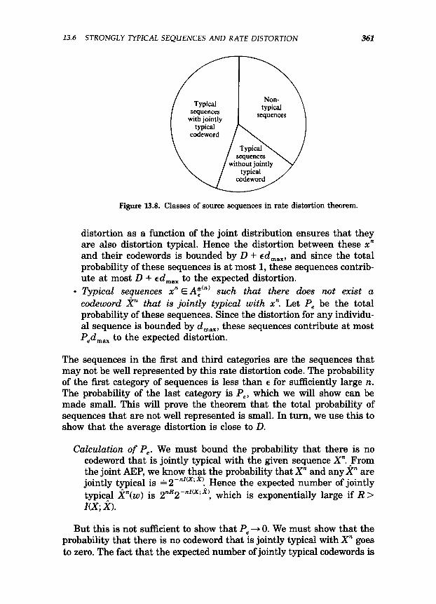
For a fixed codebook %, we divide the sequences xn E 8?” into three categories as shown in Figure 13.8.
l The non-typical sequences xnFAe . I(n) The total probability of these sequences can be made less than E by choosing n large enough. Since the individual distortion between any two sequences is boun- ded by d,,,, the non-typical sequences can contribute at most Ed,,, to the expected distortion.
l Typical sequences xn E AT’“’ such that there exists a codeword &’ that is jointly typical with x”. In this case, since the source sequence and the codeword are strongly jointly typical, the continuity of the
13.6 STRONGLY TYHCAL SEQUENCES AND RATE DISTORTlON 361
Figure 13.8. Classes of source sequences in rate distortion theorem.
distortion as a function of the joint distribution ensures that they are also distortion typical. Hence the distortion between these xn and their codewords is bounded by D + Ed,,,, and since the total probability of these sequences is at most 1, these sequences contrib- ute at most D + ~d,,.,~~ to the expected distortion.
l Typical sequences xn E AT’“’ such that there does not exist a codeword p that is jointly typical with x”. Let P, be the total probability of these sequences. Since the distortion for any individu- al sequence is bounded by d,,,, these sequences contribute at most P,4nax to the expected distortion.
The sequences in the first and third categories are the sequences that may not be well represented by this rate distortion code. The probability of the first category of sequences is less than E for sufficiently large n. The probability of the last category is P,, which we will show can be made small. This will prove the theorem that the total probability of sequences that are not well represented is small. In turn, we use this to show that the average distortion is close to D.
Cakulation of P,. We must bound the probability that there is no codeword that is jointly typical with the given sequence X”. From the joint AEP, we know that the probability that X” and any x” are jointly typical is A 2-nz(x’ “!- Hence the expected number of jointly typical x”(w) is 2nR2-nz’x’x’, which is exponentially large if R > I(X, X).
But this is not sufficient to show that P, + 0. We must show that the probability that there is no codeword that is jointly typical with X” goes to zero. The fact that the expected number of jointly typical codewords is
362 RATE DISTORTION THEORY
exponentially large does not ensure that there will at least one with high probability.
Just as in (13.93), we can expand the probability of error as
I’, = c p(xn)[l - Pr((x”, ?, E Afn))12”R . xn EAT(~)
(13.112)
From Lemma 13.6.2, we have
Substituting this in (13.112) and using the inequality (1 - x)” 5 eVnx, we have
(13.114)
which goes to 0 as n + a if R > 1(X, & + Ed. Hence for an appropriate choice of E and n, we can get the total probability of all badly repre- sented sequences to be as small as we want. Not only is the expected distortion close to D, but with probability going to 1, we will find a codeword whose distortion with respect to the given sequence is less than D+6. Cl
13.7 CHARACTERIZATION OF THE RATE DISTORTION FUNCTION
We have defined the information rate distortion function as
R(D)= min m a , (13.115) Polx):q+)P Wq(ildd(z, i&D
where the minimization is over all conditional distributions @Ix) for which the joint distribution p(~)&?Ix) satisfies the expected distortion constraint. This is a standard minimization problem of a convex func- tion over the convex set of all q(i 1~) I 0 satisfying C, &IX) = 1 for all x and CQ(~~X)JI(X)C&X, i) 5 D.
We can use the method of Lagrange multipliers to find the solution. We set up the functional
J(q) = c c p(x)q(iIx) log qG Ix> x i c
X
p(x)q(iIx) + A T c PWW~k a 32 (13.116)
(13.117)
13.7 CHARACTERIZATlON OF THE RATE DISTORTION FUNCTlON 363
where the last term corresponds to the constraint that @Ix) is a conditional probability mass function. If we let q(i) = C, p(x)q(iIx) be the distribution on X induced by &C lx), we can rewrite J(a) as
J(q) = c c pWqG Ix> log $ + AC c p(x)q(iIx)&x, i) (13.118) x i 2 i
+ c dx>C qelx) - (13.119) x i
DifYerentiating with respect to &fix), we have
+pw - c p(r’)q(~lx’)--&p~x) + Ap(xMx, i) x’
+ v(x) = 0 . (13.120)
Setting log p(x) = ~(x>/p(x>, we obtain
p(x)[ log s + h&x, i> + log /&L(x) 1 = 0 (13.121)
(13.122)
Since C, q(i(x) = 1, we must have
p(x) = 2 q(i)e-*d’“, i, P
(13.123)
q@e -Ad(x, i)
qcqx) = c, q(i)e-Wd l
Multiplying this by p(x) and summing over all x, we obtain
-hd(x, i)
q(i) = q(i) 2 p(x)e r c;, q(~t)e-kW” ’
If q(i) > 0, we can divide both sides by q(i) and obtain
p&k -I\d(r, i)
c z c,, q(~/)e-WW = 1
(13.124)
(13.125)
(13.126)
for all i E &‘. We can combine these @‘I equations with the equation
364 RATE DISTORTION THEORY
defining the distortion and calculate h and the I@ unknowns q(i). We can use this and (13.124) to find the optimum conditional distribution.
The above analysis is valid if all the output symbols are active, i.e., q(i) > 0 for all i. But this is not necessarily the case. We would then have to apply the Kuhn-Tucker conditions to characterize the minimum. The inequality condition a(i) > 0 is covered by the Kuhn-Tucker condi- tions, which reduce to
aJ =0 if q(iJz)>O,
aq(ild 20 if q(iJx)=O. (13.127)
Substituting the value of the derivative, we obtain the conditions for the minimum as
p(de -A&x, i)
c x & q(~‘)e-Ad’“, i’) =1 if q(i)>O,
p We -h&x, if)
c x c;, q(Jl’)e-“d’“’ i’) sl if q(i) = 0 .
(13.128)
(13.129)
This characterization will enable us to check if a given q(i) is a solution to the minimization problem. However, it is not easy to solve for the optimum output distribution from these equations. In the next section, we provide an iterative algorithm for computing the rate distortion function. This algorithm is a special case of a general algorithm for finding the minimum relative entropy distance between two convex sets of probability densities.
13.8 COMPUTATION OF CHANNEL CAPACITY AND THE RATE DISTORTION FUNCTION
Consider the following problem: Given two convex sets A and B in .% n as shown in Figure 13.9, we would like to the find the minimum distance between them
d min = aEyipE, &a, b) , (13.130) ,
where d(a, b) is the Euclidean distance between a and b. An intuitively obvious algorithm to do this would be to take any point x E A, and find the y E B that is closest to it. Then fix this y and find the closest point in A. Repeating this process, it is clear that the distance decreases at each stage. Does it converge to the minimum distance between the two sets? Csiszhr and Tusnady [85] have shown that if the sets are convex and if the distance satisfies certain conditions, then this alternating minimiza-
13.8 COMPUTATION OF CHANNEL CAPACITY 365
Figure 13.9. Distance between convex sets.
tion algorithm will indeed converge to the minimum. In particular, if the sets are sets of probability distributions and the distance measure is the relative entropy, then the algorithm does converge to the the minimum relative entropy between the two sets of distributions.
To apply this algorithm to rate distortion, we have to rewrite the rate distortion function as a minimum of the relative entropy between two sets. We begin with a simple lemma:
Lemma X3.8.1: Let p(x)p( ylx) be a given joint distribution. Then the distribution r(y) that minimizes the relative entropy D( p(x)p( yIx)ll p(x) r(y)) is the marginal distribution r*(y) corresponding to p( ~1x1, i.e.,
D(p(x)p(y(x)l(p(x)r*(y)) = 7% D(p(dp( yIdIIpW-( yN , (13.131)
where r*(y) = C, p(x)p( y lx). Also
ZE Fy PWP(Y Id log $$ = c p(x)p( ylx) log $$ , (13.132) , x9 Y
pWp( y Id r*(3cly) = c, p(x)p( y Jx) *
proof:
D( pWp( yldJI pWr( yN - D(pWp( yIx)ll pWr*( yN
(13.133)
= c PCX)P(Y lx> log $g;;jy (13.134) x9 Y
366 RATE DISTORTION THEORY
(13.136)
(13.137)
10. (13.139)
The proof of the second part of the lemma is left as an exercise. cl
We can use this lemma to rewrite the minimization in the definition of the rate distortion function as a double minimization,
R(D) = min min 2 2 p(3G)q(32~x)log $i!$ l
r(i) q(iJx): c p(x)q(iIx)d(x, 3iMD z p
(13.140)
If A is the set of all joint distributions with marginal p(x) that satisfy the distortion constraints and if B the set of product distributions p(~)r($ with arbitrary r(i), then we can write
We now apply the process of alternating minimization, which is called the Blahut-Arimoto algorithm in this case. We begin with a choice of A and an initial output distribution r(i) and calculate the q(ilx) that minimizes the mutual information subject to a distortion constraint. We can use the method of Lagrange multipliers for this minimization to obtain
r(i)e -h&x, i)
q(qx) = c; r(.$e-wG) . (13.142)
For this conditional distribution q(ilx), we calculate the output dis- tribution r(32) that minimizes the mutual information, which by Lemma 13.31 is
(13.143)
We use this output distribution as the starting point of the next iteration. Each step in the iteration, minimizing over q( l I l ) and then minimizing over r( l > reduces the right hand side of (13.140). Thus there is a limit, and the limit has been shown to be R(D) by Csiszar [791,
SUMMARY OF CHAPTER 13 367
where the value of D and R(D 1 depends on h. Thus choosing A appropri- ately sweeps out the R(D) curve.
A similar procedure can be applied to the calculation of channel capacity. Again we rewrite the definition of channel capacity,
(13.144)
as a double maximization using Lemma 13.8.1,
&lY) c = Fx$YF c c r(jc)p(yld log r(x) .
32 Y (13.145)
In this case, the Csiszar-Tusnady algorithm becomes one of alternating maximization-we start with a guess of the maximizing distribution r(x) and find the best conditional distribution, which is, by Lemma 13.8.1,
(13.146)
For this conditional distribution, we find the best input distribution r(x) by solving the constrained maximization problem with Lagrange multi- pliers. The optimum input distribution is
which we can use as the basis for the next iteration. These algorithms for the computation of the channel capacity and the
rate distortion function were established by Blahut [37] and Arimoto [ll] and the convergence for the rate distortion computation was proved by Csiszar [79]. The alternating minimization procedure of Csiszar and Tusnady can be specialized to many other situations as well, including the EM algorithm [88], and the algorithm for finding the log-optimal portfolio for a stock market 1641.
SUMMARY OF CHAPTER 13
Rate distortion: The rate distortion function for a source X-p(r) and distortion measure d(x, i) is
R(D) = min 1(x; a , (13.148) p(Xlx): C(,,i) p(x)p(iIx)d(x, i)SD
368 RATE DZSTORTZON THEORY
where the minimization is over all conditional distributions p(i]x) for which the joint distribution p(r, i) = p(x)p(~~;lx> satisfies the expected distortion constraint.
Rate distortion theorem: If R > R(D), there exists a sequence of codes &X”) with number of codewords IXY l )I I 2”R with E&X”, X’YX”))-, D. If R <R(D), no such codes exist.
Bernoulli source: For a Bernoulli source with Hamming distortion,
R(D)=H(p)-H(D). (13.149)
Gaussian source: For a Gaussian source with squared error distortion,
R(D)=;log$. (13.150)
Multivariate Gaussian source: The rate distortion function for a mul- tivariate normal vector with Euclidean mean squared error distortion is given by reverse water-filling on the eigenvalues.
PROBLEMS FOR CHAPTER 13
1. One bit quantization of a single Gaussian random variable. Let X- Jw, a21 and let the distortion measure be squared error. Here we do not allow block descriptions. Show that the optimum reproduction points for 1 bit quantization are -+ flu, and that the expected distortion for 1 bit quantization is %? a”.
Compare this with the distortion rate bound D = a22 -2R for R = 1.
2. Rate distortion function wit? infinite distortion. Find the rate distortion function R(D) = min 1(X, X) for X - Bernoulli ( i ) and distortion
1
0, x=i, d(Q)= 1, x=l,i=O,
00, x=0$=1.
3. Rate distortion for binary source with asymmetric distortion. Fix p(xli) and evaluate 1(X,X) and D for
X- Bern(l/2),
0 a d(x,c,)= b o . [ I
(R(D) cannot be expressed in closed form.)
4. Properties of R(D). Consider a discrete source X E %’ = { 1,2, . . . , m} with distribution pl, p2, . . . , p, and a distortion measure d(i, j). Let R(D) be the rate distortion function for this source and distortion measure. Let d’(i, j) = d(i, j) - wi be a new distortion measure and
PROBLEMS FOR CHAPTER 33 369
let R’(D) be the corresponding rate distortion function. Show that R’(D) = R(D + W ), where ti = C piwi, and use this to show that there is no essential loss of generality in assuming that min, c&i, i) = 0, i.e., for each x E 8, there is one symbol 2 which reproduces the source with zero distortion.
This result is due to Pinkston [209].
5. Rate distortion for uniform source with Hamming distortion. Consider a source X uniformly distributed on the set { 1,2, . . . , m}. Find the rate distortion function for this source with Hamming distortion, i.e.,
d(x, i) = {
0 ifx=i, 1 ifx#i.
6. Shannon lower bound for the rate distortion function. Consider a source X with a distortion measure d(x, i) that satisfies the following proper- ty: all columns of the distortion matrix are permutations of the set W,, 4,. . . , d,}. Define the function
4(D)= glax H(p). P’Cizl PidisD
(13.151)
The Shannon lower bound on the rate distortion function [245] is proved by the following steps: (a) Show that 4(D) is a concave function of D. (b) Justify th e following series of inequalities for 1(X; X) if
Ed(X, k) 5 D,
1(x; % = H(X) - H(X@) (13.152)
= H(X) - 2 p(i)H(X@ = i) i
(13.153)
1 H(X) - c p(i)+(D,) i
(13.154)
(13.155)
rH(X)- 4(D), (13.156)
where Di = C, p(x]i)d(x, i). (c) Argue that
R(DkH(X)-4(D), (13.157)
which is the Shannon lower bound on the rate distortion function. (d) If in add t i ion, we assume that the source has a uniform dis-
tribution and that the rows of the distortion matrix are permuta- tions of each other, then R(D) = H(X) - 4(D), i.e., the lower bound is tight.
370 RATE DlSTORTlON THEORY
7. Erasure distortion. Consider X- Bernoulli( i ), and let the distortion measure be given by the matrix
Calculate the rate distortion function for this source. Can you suggest a simple scheme to achieve any value of the rate distortion function for this source?
8. Bounds on the rate distortion function for squared error distortion. For the case of a continuous random variable X with mean zero and variance a2 and squared error distortion, show that
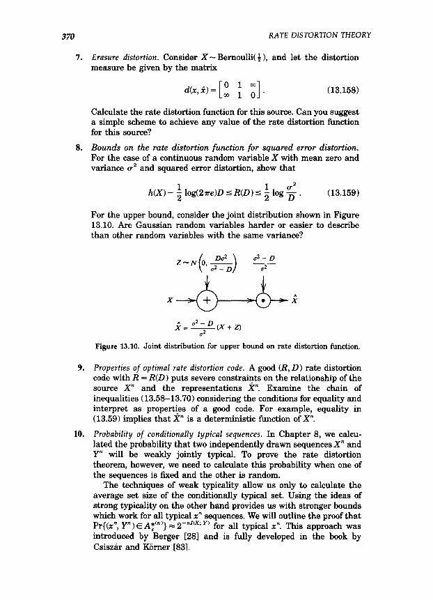
h(X) - i log(2?re)D I R(D) I f log $ . (13.159)
For the upper bound, consider the joint distribution shown in Figure 13.10. Are Gaussian random variables harder or easier to describe than other random variables with the same variance?
Figure 13.10. Joint distribution for upper bound on rate distortion function.
9. Properties of optimal rate distortion code. A good (R, D) rate distortion code with R = R(D) puts severe constraints on the relationship of the source X” and the representations x”. Examine the chain of inequalities (13.58-13.70) considering the conditions for equality and interpret as properties of a good code. For example, equality in (13.59) implies that p is a deterministic function of X”.
10. Probability of conditionally typical sequences. In Chapter 8, we calcu- lated the probability that two independently drawn sequences X” and Y” will be weakly jointly typical. To prove the rate distortion theorem, however, we need to calculate this probability when one of the sequences is fixed and the other is random.
The techniques of weak typicality allow us only to calculate the average set size of the conditionally typical set. Using the ideas of strong typicality on the other hand provides us with stronger bounds which work for all typical X” sequences. We will outline the proof that Pr{(x”, Y”) E AT’“‘} = 2-nz(X’ y, for all typical x~. This approach was introduced by Berger [28] and is fully developed in the book by Csiszar and Korner [83].
PROBLEMS FOR CHAPTER 13 371
Let (Xi, Yi> be drawn i.i.d. -p(z, y). Let the marginals of X and Y be p(x) and p(y) respectively. (a) Let A*(“) be the strongly typical set for X. Show that c
IA;‘“‘I & 2nH(X) (13.160)
Hint: Theorem 12.1.1 and 12.1.3. (b) The joint type of a pair of sequences W, y” ) is the proportion of
times (xi, yi) = (a, b) in the pair of sequences, i.e.,
pxn,Yn(a, b) = $(a, b( x”, y”) = i &$,I I(xi = a, yi = b) * (13.161)
The conditional type of a sequence y” given xR is a stochastic matrix that gives the proportion of times a particular element of 9 occurred with each element of 8 in the pair of sequences. Specifically, the conditional type V,,,,,(b Icz) is defined as
Nb, blx”, Y”) V,~,,dbb) = jQlxn) * (13.162)
Show that the number of conditional types is bounded by (n + l)l”lPl .
(c) The set of sequences y” E 9” with conditional type V with respect to a sequence zn is called the conditional type class Tv(x” ). Show that
(d) The sequence yn E W is said to be e-strongly conditionally typical with the sequence xn with respect to the conditional distribution V( - I . ) if the conditional type is close to V. The conditional type should satisfy the following two conditions: i. For all (a, b) E aP x 91 with V(bla)> 0,
; IN(a, blx: y”) - V(bla)N(alx”)l~ 6 . (13.164)
ii. N(a, blx”, y”) = 0 for all (a, b) such that V(bla) = 0.
The set of such sequences is called the conditionally typical set and is denoted AT’“’ (Ylx”). Show that the number of sequences y” that are conditionally typical with a given xn E ZP is bounded by
?t(W(Y(X)-cl) I IA;‘“‘(ylx”)l 5 (n + l)1~11~Y12n(N(Y1X)+cl) ,
(13.165) where E~--,O as E+O.
372 RATE DZSTORTION THEORY
(e) For a pair of random variables (X, Y) with joint distribution p(x, y), the e-strongly typical set AT’“’ is the set of sequences (x”, y”) E En X ??/” satisfying i.
/ iN(a, blx”, Y”) --da, WI< & (13.166)
for every pair (a, b) E %’ x 3 with p(a, b) > 0. ii. N(a,b~x~,y”)=Oforall(a,b)~%‘~~withp(a,b)=O.
The set of E-strongly jointly typical sequences is called the E- strongly jointly typical set and is denoted Af”‘(X, Y). Let (X, Y) be drawn i.i.d. -p(x, y). For any xn such that there exists at least one pair (x”, y”) E AT’“‘(X, Y), the set of sequences y” such that (x”, y”) EAT(~) satisfies
(n + ;),%,,%, 2n(H(YIX)-G(c)) I I{ yR: (x”, y”) E AT’“‘} 1
I(n + 1) I~11912n(H(YlX)+S(s)) ,
(13.167)
where US+ 0 as E + 0. In particular, we can write
2 n(ff(YIX)-+ I I{yn:(xn, y”) eAT( 5 24H(Y1X)+4,
(13.168)
where we can make Q. arbitrarily small with an appropriate choice of E and n.
(f) Let Y1, Y2,. . . , Y, be drawn i.i.d. -np(yi>. For xn EA:(~‘, the probability that (x”, Y”) E AT’“’ is bounded by
The idea of rate distortion was introduced by Shannon in his original paper [238]. He returned to it and dealt with it exhaustively in his 1959 paper [245], which proved the first rate distortion theorem. Meanwhile, Kolmogorov and his school in the Soviet Union began to develop rate distortion theory in 1956. Stronger versions of the rate-distortion theorem have been proved for more general sources in the comprehensive book by Berger [27].
HISTORXAL NOTES 373
The inverse water-filling solution for the rate-distortion function for parallel Gaussian sources was established by McDonald and Schultheiss [190]. An itera- tive algorithm for the calculation of the rate distortion function for a general i.i.d. source and arbitrary distortion measure was described by Blahut [37] and Arimoto [ll] and Csiszar [79]. This algorithm is a special case of general alternating minimization algorithm due to Csiszar and Tusnady [85].