Page 1
1
Rating History and the Rating Dynamics of Fallen Angels, Rising Stars, and Big
Rating Jumpers
Huong Dang1 and Graham Partington
University of Sydney
30 April, 2008
Abstract
Using samples from Standard & Poor’s CreditPro 2005 dataset, we estimate
models of rating migration subsequent to firms that issue bonds becoming fallen angels
(FAs), becoming rising stars (RSs), or experiencing historical rating jumps of at least
two notches (big rating jumpers). Comparator issuers (peers) are identified for the
foregoing groups and rating transition models are estimated for these peers. The results
suggest that different models of rating transition may be needed for fallen angels, rising
stars and big jumpers relative to their peers. In general, the impact of rating history on
the probability of a rating transition varies according to the rating path that occurred
prior to the current rating state.
JEL classification: C13, C14, C32, C34, C41, G14
Keywords: Survival analysis, proportional hazards, rating migration, rating history,
non-Markovian behaviors, fallen angels, rising stars, big rating jumps.
1 Corresponding author: Huong Dang. Email: [email protected] ; Tel.: +61 421 523 259; Fax: +61 2 93516461. The authors wish to thank Paul Allison for advice and Capital Market Cooperative Research Center for financial support
Page 2
2
1. Introduction
Estimates of rating migration probabilities are important to the profitability of
fixed income investments, to credit pricing decisions, and also to credit risk
management and capital adequacy requirements under the BASEL II framework.
Previous research suggests that rating migrations depend on rating history, for example
the direction of a prior rating change impacts on the current migration probability,
Hamilton and Cantor (2004). Given this dependence on rating history it is natural to ask
whether one model fits all, or whether differing paths for rating history lead to different
models. For example, do fallen angels exhibit the same dependence on rating history as
other bonds? We estimate models of rating migration subsequent to firms that issue
bonds becoming fallen angels, becoming rising stars, or experiencing historical rating
jumps of at least two notches (big jumpers.) Comparator issuers (peers) are identified
for the foregoing groups and rating transition models are estimated for these peers. For
example, fallen angels with a speculative grade that are further downgraded are
compared to other speculative grade issuers experiencing a downgrade.
The modelling of rating transitions has received substantial attention in the
research literature. However, there has been little work that investigates non-Markovian
rating dynamics for fallen angels, rising stars, and big jumpers. Comparing rating
transition models for these issuers with the models for their peers, the results show that
the significant variables differ. Furthermore, relative to their comparators, rating
transitions for fallen angels, rising stars and big rating jumpers, generally show more
dependence on rating history. The implication is that bond investors, banking
institutions and regulators, may need to consider conditioning their models of transition
probability on the path the issuer has followed to its current rating. If, for example, the
Page 3
3
issuer is a fallen angel then it may need a fallen angel model to get appropriate
transition probabilities.
The paper is structured as follows: Section 2 provides a brief discussion of the
literature. Section 3 presents the methods used, followed by a description of the data in
Section 4. Section 5 summarizes the results of the estimation models. Section 6
summarizes the main findings of this research.
2. Literature Review
2.1. Non-Markovian behaviour
Previous empirical studies have found evidence of non-Markovian behaviours
such as duration dependence, serial correlation, and path dependence in rating
dynamics. For example, Atlman and Kao (1992) and Carty and Fons (1994) provided
evidence of serial correlation in rating migrations. Lando and Skodeberg (2002)
indicated that there is a negative relation between the migration probability and the
length of time an issuer stayed in a particular rating. Hamilton and Cantor (2004)
suggested that the direction of a prior rating change impacts on the migration
probability. Figlewski, Frydman, and Liang (2006) also suggested that rating
momentum exists, that is, a downgrade is more likely to be followed by a further
downgrade than an upgrade. Altman (1998) found that newly rated firms, compared
with seasoned firms of the same rating class, exhibit a smaller probability of rating
migrations within a few years. Figlewski et al (2006) also provided evidence of an
ageing effect. Specifically, the longer it is since a firm was first rated, the more likely it
is that the firm would default.
Page 4
4
2.2. Fallen Angels
Moody’s study on fallen angels over the period 1982-2003 (Mann, Hamilton,
Varma, and Cantor, 2003) found that fallen angels have higher probabilities of being
upgraded to investment grade than their peers. Standard & Poors’ study on fallen
angels (Vazza, Aurora, Schneck, 2005) also found the same result. Mann et al. also
reported that the ratings fallen angels received, at the time they were downgraded from
investment to speculative grade, affected their default probability as well as their
probability of returning to an investment grade.
3. Method
3.1. Hazards
The effect of rating history covariates on the duration of a rating grade is
investigated using survival analysis. The resulting survivor function S(t) =P (T>t) gives
the probability that the time of a rating transition T will exceed time t, conditional on
variables that capture the firm’s rating history. The survivor function can be
conveniently derived from the hazard function. The hazard, roughly speaking, gives the
expected rate of incidence of a rating transition over a short interval.3 The hazard
function is estimated using Cox’s (1972) proportional hazards model.
3.2. Rating states and estimation
The focus of this study is the probability that a rating state for an issuer will
change. The time in a rating state starts from the time the firm enters a rating class
(starting rating) subsequent to the commencement date of the study (1 January, 1982).
The state ends at the time the firm migrates to another rating class (ending rating). The
time a firm keeps the same rating is the survival time and time is measured in years.
3 The inverse of the hazard gives the expected duration conditional on survival until the start of period t.
Page 5
5
If a firm exits from a rating class due to merger, extinction of firm’s rated debt,
the debt becoming unrated (NR), or any reason other than an up-grade or a down-grade,
the survival time is treated as censored. In the upgrade model, down-state transitions
(rating states with starting ratings better than ending ratings.) are censored and vice
versa for downgrade models. Rating states commencing before the start of the model
estimation period, or finishing after the end of the model estimation period, are also
treated as censored.
The rating states are pooled for the period 1982-2005. Hazard models are then
developed for the following sub-samples:
Fallen angels and their speculative grade rated peers
Rising stars and their investment grade rated peers
Firms with a previous big down jump in rating and their peers
Firms with a previous big up jump in rating and their peers
The use of repeated rating transitions for the same firm is likely to introduce
dependence among the observations. This problem is reduced to the extent that
covariates in the model control for dependence. To allow for any dependence, the Wei-
Lin-Weissfeld method (Wei, Lin, Weissfeld, 1989) is used to get robust variance
estimates. This method, however, does not correct for any bias in the coefficients. To
account for ties, in which several firms experience the same rating migration event with
the same survival period, it has been traditional to use approximation adjustments such
as the Efron method. However, we use the exact method for handling ties provided in
SAS Version 9.
3.3. The Model
The model to be estimated is:
Page 6
6
h(Z,t) = h(0,t) expZβ
Where h(Z,t) is the hazard for a rating transition at time t given the covariate
vector Z.
h(0,t) is the baseline hazard
β is the vector of estimated coefficients
The covariate vector Z contains the following variables, selected primarily on
the basis of their significance in the prior ratings literature. However, some variables
such as the length of lagged states and rate of prior changes in ratings are analogous to
variables that Yao, Partington and Stevenson (2005) found significant in studying
transitions in runs of stock prices.
Lag one: The duration (in years) of the non-censored state (with start rating different
from ending rating) immediately preceding the current state (LAG_ONE).
Lag two: The duration (in years) of the non-censored state (with start rating different
from ending rating) immediately preceding the lag one state (LAG_TWO).
Rate of prior rating change: This rate equals the number of rating changes observed
between the entry of the firm to the study and the beginning of the current state divided
by the period over which the changes were observed (RATE_PRIOR_CHANGE).
Original rating: the rating of the firm when it was first rated (ORIGINAL_RATING).
Start rating: The rating at the beginning of each rating state (START_RATING).
Age since first rated: The rating age of the firm, which is equal to the length in years
from the time the firm was first rated until the beginning of the current state
(AGE_SINCE_FIRST_RATED).
Page 7
7
A prior not rated (NR) status: This variable takes the value of one if the firm
experienced a NR status from the time it entered the study until the beginning of the
current rating state, otherwise it is zero (DUMMY_NR).
A switch from an investment to a speculative (junk) grade: This variable takes the
value of one if immediately prior non-censored rating state underwent a switch from an
investment to a junk grade (fallen angel). This dummy variable indicates whether the
rating state analyzed was a fallen angel (DUMMY_INV_JUNK_SWITCH).
A switch from a speculative (junk) to an investment grade: This variable takes the
value of one if immediately prior non-censored rating state underwent a switch from a
junk to an investment grade (rising star). This dummy variable indicates whether the
rating state analyzed was a rising star (DUMMY_JUNK_INV_SWITCH).
We examine whether the start rating proximity to the investment / junk boundary states
impacts on the upgrade / downgrade hazards of the issuers studied. Two dummy
variables were used for this purpose. If the start rating of the current state is in the
lower investment boundary, BBB-, BBB, BBB+, the dummy variable takes the value
one, otherwise zero (DUMMY_SR_LOWER_INV), or if the start rating is in the junk
boundary, BB-, BB, BB+ , the dummy takes the value one, otherwise zero
(DUMMY_SR_JUNK_BOUNDARY).
Dummy variables were also created as control variables representing the industry sector
of each firm. Thirteen sectors were categorized by Standard & Poor’s in the
CreditPro2005 dataset. Firms in the financial institution sector were excluded from the
sample leaving twelve industry sectors. The firm’s industry dummy is coded one if it was
in the sector and zero otherwise. The insurance sector was left un-coded in order to avoid
perfect collinearity in the industry dummies. The industry sectors are listed in Table 1.
Page 8
8
Unlike most studies on rating dynamics, which just focuses on the coarser rating
categories (AAA, AA), we employ finer rating sub-categories such as AAA, AAA-.
The rating scales, which take into account plus and minus signs, are coded from 0 to 26
with 0 indicating the default state (D) and 26 indicating the AAA state. Details of the
rating codes are provided in Table 1. The higher the value of a rating variable (original
rating, start rating), the better the quality of the firm at the corresponding time. A similar
coding technique was employed by Kim and Wu (2006) to examine the impacts of
sovereign credit ratings history on international capital inflows to emerging countries,
and on the development of the financial sectors in these countries. The numeric
conversion maintains the rank order of the rating but assumes that the difference between
any two consecutive rating states is the same. The alternative of coding each rating class
through dummy variables would consume a substantial number of degrees of freedom
and would also hinder clear and compact presentation of the results.
TABLE 1 HERE
4. Data
Rating data was obtained from Standard & Poor’s CreditPro2005. The rating
behavior of US’s fallen angels, rising stars, and big jumpers is examined over the time
horizon 1982 – 2005. This period covered different phases of the credit and business
cycles in the US.
The high yield bond market in the US was established as a substantial market in
the first half of the 1980s. The year 1986 saw a record of 52 fallen angels representing
4.21% of investment grade issuers that year, Standard and Poors (2005). Rating
Page 9
9
migrations consequent to the establishment of the high yield bond market from the
middle of the 1980s constitute an important source of events for the study.
The period 1990 to 2005 covers one full business cycle for the US and many
developed markets. The period started with a recessionary year followed by a long
expansion in the US economy. There was a growth in rising stars which peaked in
1997. Since then the number of rising stars has been declining and has been
outnumbered by fallen angels. The incidence of fallen angels steadily increased during
the economic slowdown in early 2000s, and peaked at 2002 with 146 fallen angels,
representing 4.65% of the 3139 investment grade issuers that year, Standard and Poors
(2005).
4.1. Fallen Angels
The dataset includes 541 fallen angel (FA) firms. These are cases which were
downgraded from investment grade to speculative (junk) grade in the non-censored
transition immediately prior to the current state. From the current state for these 541
fallen angels, 278 experience further downgrades (FA down states), 62 undergo an up-
grade but remain junk rated (FA up-to-junk states), and 89 experience an up-grade to
investment rated (FA up-to-investment states).
Peer group samples were established as follows. A random sample of 541
speculative (junk) rated issuer states was selected as a peer group for the fallen angels.
These peers were sampled from issuers that had not experienced a FA event but had a
junk rating. From the current state for these 541 speculative grade rated peers, 264
undergo down-grades (peers of FAs down-states), 91 experience up-grades to junk
classes (Peers of FAs up-to-junk states), 34 undergo up-grades to investment classes
Page 10
10
(peers of FA up-to-investment states). Statistics for state lengths of fallen angels and
their peers are given in Table 4.
TABLE 4 HERE
4.2. Rising stars
The dataset includes 429 rising star (RS) states, which were recently upgraded
from junk to investment grade immediately prior to the current state. From the current
state for these 429 rising stars, 153 experience upgrades (RS up states), 76 undergo a
down-grade back to junk rated (RS down-to-junk states), and 35 experience a down-
grade but remain investment rated (RS down-to-investment states).
Peer group samples were established as follows. A random sample of 429
investment grade rated issuer states was selected., These peers were sampled from
issuers that had not experienced a RS event but were rated investment classes. From the
current state for these 429 investment grades rated peers, 88 undergo up-grades (peers of
RS up-states), 12 experience down-grades to junk classes (Peers of RS down-to-junk
states), 201 undergo down-grades to investment classes (peers of RS down-to-
investment states). Statistics for state lengths of rising stars and their peers are given in
Table 5.
TABLE 5 HERE
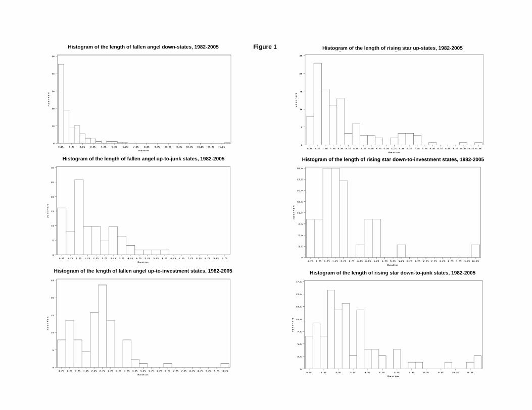
Histograms of state lengths of fallen angels and rising stars are depicted in
Figure1. Both FA and RS distributions tend to have a positive skew.. For fallen angels,
the histograms suggest that further declines in credit rating tend to be swift, while
Page 11
11
improvements tend to take much longer. In contrast, for rising stars improvements in
ratings tend to happen more quickly than worsening ratings.
FIGURE 1 HERE
4.3. Big down jumpers
We define a big down jumper as a firm who recently experienced a big down
jump in credit rating of at least two notches in their non-censored rating transitions
immediately prior to the current rating. The dataset includes 2088 big down jumpers, of
which 1317 subsequently experience down-grades and 400 subsequently experience up-
grades.
The peer group for the big down jumper sample includes 2088 issuer states.
These peer issuer states have experienced a lag one down state but not a lag one big
down jump. Of the 2088 peers, 1124 end in down-grade states (peers of big down jump
down states) and 329 end in up-grade states (peers of big down jump up-states). Statistics
for state lengths of big down jumpers and their peers are given in Table 3.
TABLE 3 HERE
4.4. Big up jumper
A big up jumper is a firm who recently experienced a big jump up in credit rating
of at least two notches. The dataset includes 769 big up jumpers, of which 233
subsequently experience down-grades and 248 subsequently experience up-grades.
The peer group for the big up jumper sample includes 769 issuer states. These
peer states have experienced a lag one up state but not a lag one big jump up. Of the 769
Page 12
12
peers , 232 are down-grade states (peers of big up jump down states) and 274 are up-
grade states (peers of big up jump up-states). Statistics for state lengths of big up
jumpers and their peers are given in Table 2.
TABLE 2 HERE
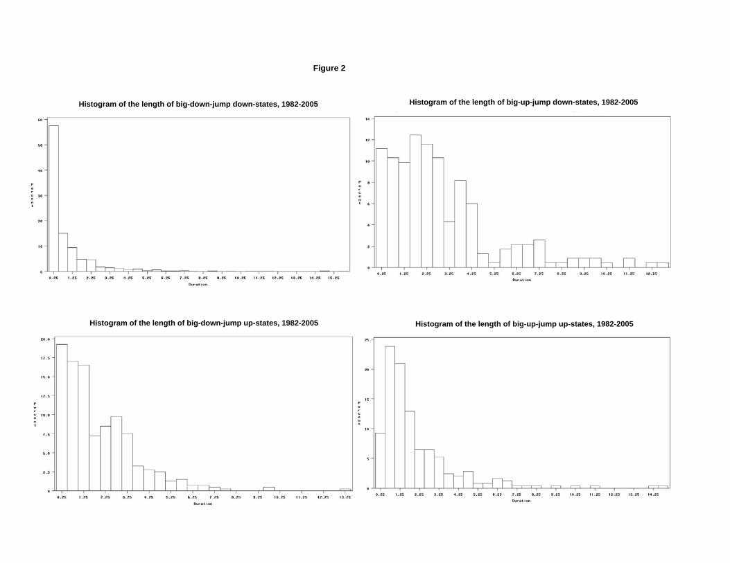
Histograms of state lengths of big down jumpers and big up jumper are depicted
in Figure 2. Both big down jumpers and big up jumpers have non normal distribution.
For big down jumpers, the histograms show a clear tendency for further downgrades to
follow quickly, but for up grades to take substantially longer. On the other hand, for big
up jumpers, transitions to down states tend to arise more slowly than transitions to up
states.
FIGURE 2 HERE
5. Results
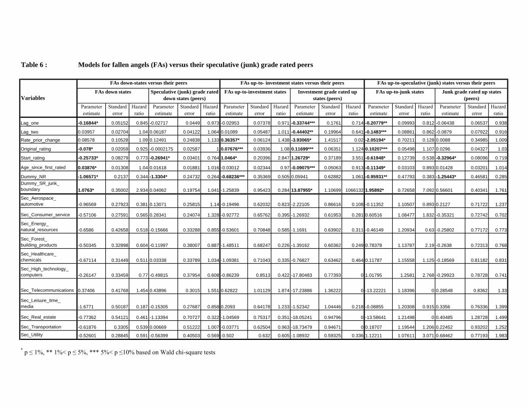
5.1. FAs, RSs and their peers.
The following model is estimated for RSs and their respective peers
h(t)=h0(t) exp { β1 Lag_one + β2 Lag_two + β3 Rate_prior_change + β4
Original_rating + β5 Start_rating + β6 Age_since_first_rated + β7 Dummy_NR
+ β8 Dummy_SR_lower_inv
11β D
k sector_kk=1+ }∑
Page 13
13
A similar model, except that the covariate dummy_SR_lower_inv is replaced by
the covariate dummy_SR_junk_boundary , is developed for FAs and their peers.
The results of the models for FAs and their peers are presented in Table 6 while
the results of the models for RSs and their peers are shown in Table 7.
TABLE 6 HERE
TABLE 7 HERE
In interpreting Table 6 and 7, a negative coefficient reduces the hazard and
therefore reduces the probability of a rating migration. For example, in the model for
peers of FA down states (Table 6), an increase in the length of the lag one rating state
by one year reduces the chance of a down-grade by (1-0.973) or 2.7%.
The impacts of rating history on the migration hazards of FAs and RSs are
markedly different from the impacts on the hazards of their respective peers. For
instance, the migration hazards of FA down states and FA up to junk states depend
significantly on several rating history covariates, whereas the hazard of their peers
depend only on their start rating (start_rating) and a prior NR status (dummy_NR).
Similarly, the migration hazards of RS down-to-junk states depend significantly on
several rating history covariates while the hazard of their peers just depends on the rate
of prior rating changes (rate_prior_change).
FAs/ RSs states and their respective peers, in some cases, are impacted in
opposite ways by certain rating history covariates. For instance, a higher rate of prior
rating change (rate_prior_change) increases the hazards of FA up-to-investment states
but decreases the hazards of their peers. An older rating age (age_since_first_rated)
increases the migration hazards of RS up-states but decreases the hazards of their peers.
Page 14
14
Regarding the impacts of significant rating history covariates on the migration
hazard of FAs and RSs states, a shorter lag one rating state (lag_one), a lower start
rating (start_rating) and being in junk boundary states BB-, BB, BB+
(Dummy_SR_junk_boundary=1) increase the hazards of FAs migrating within their
junk states. A better original rating will increase the up-grade hazards of FAs and
decrease the down-grade hazards of RSs. The older the RS is (age_since_first_rated),
the higher the hazards of RS migrating within their investment states.
5.2. Big up/ big down jumper and their respective peers
The following model is developed for big up jumpers and their respective peers
r(t)=r0(t) exp { β1 Lag_one + β2 Lag_two + β3 Rate_prior_change + β4
Original_rating + β5 Start_rating + β6 Age_since_first_rated + β7 Dummy_NR
+ β8 Dummy_SR_junk_boundary + + β9 Dummy_junk_inv_switch + β10
Dummy_SR_junk_boundary + β11 Dummy_SR_lower_inv
11β D
k sector_kk=1+ }∑
A similar model, except that the covariate dummy_junk_inv_switch is replaced
by the covariate dummy_inv_junk_switch, is developed for big down jumpers and their
respective peers
The results of the models for rating states with historical big up jumps / big
down jumps and their peers are presented in Table 8.
TABLE 8 HERE
Page 15
15
First of all, big jumpers down states are more affected by their rating history
than are their respective peers. For instance, original rating (original_rating) has a
significant negative impact on the hazards of big jumpers down states but no effect on
their peers. On the other hand, up states with a historical big up jump are less
influenced by the rating history compared with their peers. For example, the length of
the lag one/ lag two rating state (lag_one, lag_two), and rating age
(age_since_first_rated) do not have significant impacts on the hazards of up-states with
a historical big up jump but do impact on their peers.
The statistically significant impacts other rating history covariates impose on
the migration hazards of big rating jumpers varies according to their rating path. For
instance, only states with a historical big down jumps and their peers are (negatively)
influenced by the length of the lag one rating state (lag_one), and only down-states with
a historical big down jump and their peers are (positively) influenced by the rate of
prior rating change (rate_prior_change). For those with a historical big up jump, being
in the boundary of speculative (junk) or investment grades reduce the migration
hazards of down-states (and their peers) but increase the hazards of up states (increase
up-grade momentum). For down states with a historical big down jump, having
experienced a switch from investment to junk grades (Fallen angels) or currently being
in the investment grade boundary reduce their migration hazards (reduce down-grade
momentum)..
6. Conclusion
Using samples from Standard & Poor’s CreditPro 2005 dataset, the Cox
proportional hazard model was used to investigate the rating dynamics of fallen angels
Page 16
16
(FA), rising stars (RS) and firms with historical big rating jumps (big rating jumpers)
over the period 1982-2005.
The results show that the impacts rating history imposed on the migration
hazards of FAs, RSs, and big rating jumpers are different from those of their peers. FAs
down states, FAs up-to-junk states, and for RS all states are more influenced by the
rating history than are their respective peers while FAs up-to-investment states are less
affected by rating history compared with their peers. Big rating jumpers and their peers
also tended to have different statistically significant predictors. In some cases, FAs,
RSs and their respective peers, were impacted in opposite ways by some rating history
covariates.
The results of this study are relevant for fixed income portfolio managers,
banking institutions and regulators. As fallen angels and big down jumpers, especially
FA down-states, FA up-to-junk states, and down-states with a historical big down
jump, show more dependence on the rating history, internal rating based models and
credit stress tests should take into account the rating path the issuer has followed to its
current rating state. Most importantly, separate hazard models should be developed to
account for the varying risk of rating changes of issuers with different historic rating
paths.
Page 17
17
References
Allison, P. D. (1984). “Event History Analysis”, Sage University Paper Series on
Quantitative Applications in the Social Sciences.
Allison, P. D. (1995). “Survival analysis using SAS A practical guide”, SAS Press
Altman, E. (1998). “The importance and subtlety of credit rating migration.” Journal of
Banking and Finance 22: 1231-1247.
Altman, E., and D. L. Kao (1992). “Rating Drift of High Yield Bonds.” Journal of
Fixed Income March: 15-20.
Altman, E., and H. Rijken (2005). “The Impact of the Rating Agencies’ Through-the-
cycle Methodology on Rating Dynamics.” Economic Notes by Banca Monte dei Paschi
di Scienna SpA 34: 127-154.
Avramov, D., G. Jostova, A. Philipov (2003). “Corporate Credit Risk Changes:
Common Factors and Firm-Level Fundamentals.”
Berd, A. (2005). “Dynamic Estimation of Credit Rating Transition Probabilities.”
Cantor, R., and C. Mann (2003). “Measuring the performance of corporate bond
ratings.” Moody’s Investor Service Special Comment, April.
Carty, L.V., and J. S. Fons (1993), “Measuring changes in corporate credit quality”,
Moody’s Special Report, New York.
Cantor, R., J. Fons, C. Mahoney, D. Watson, and K. Pinkes (1999). “The evolving
meaning of Moody’s bond ratings.” Moody’s Investor Service Rating Methodology
August.
Carty, L. (1997). “Moody’s Rating Migration and Credit Quality Correlation, 1920-
1996.” Moody’s Investor Service Special Comment, July
Page 18
18
Choy, E., S. Gray, V. Ragunathan (2006). “Effect of credit rating changes on
Australian stock returns.” Journal of Accounting and Finance 46: 755-769.
Cox, D. (1972). “Regression Models and Life Tables.” Journal of Royal Statistical
Society Series B (Methodological) 34: 187-220.
Cox D., a. D. O. (1984). Analysis of Survival Data, Chapman & Hall, London.
Dang, H., and G. Partington (2007a), Modelling Rating Migrations, International C.R.E.D.I.T
Conference on Credit Rating, Venice, September.
Dang, H. and G. Partington (2007b), Rating Migrations: The Effect of Rating History and Time,
Australasian Finance and Banking Conference, December.
Figlewski, S., H. Frydman, W. Liang (2006). “Modeling the Effects of Macroeconomic
Factors on Corporate Default and Credit Rating Transitions.”
Frydman, H., and T. Schuermann (2006). “Credit ratings dynamics and Markov
mixture models.” Working paper.
Gonzalez, F., F. Haas, R. Johannes, M. Persson, L. Toledo, R. Violi, M. Wieland, and
C. Zins (2004). “Market dynamics associated with credit ratings: a literature review.”
Occasional paper series (European Central Bank) 16.
Hamilton, D., P. Varma, S. Ou, and R. Cantor (2006). “Default and recovery rates of
corporate bond issuers, 1920-2005.” Moody’s Investor Service Special Comment,
March.
Hamilton, D., R. Cantor (2004). “Rating transitions and default conditional on
watchlist, outlook and rating history.” Moody’s Investor Service Special Comment,
February.
Page 19
19
Helwege, J., and P. Kleiman (1996). “Understanding Aggregate Default Rates of High
Yield Bonds.” Federal Reserve Bank of New York Current Issues in Economics and
Finance 2: 1-6.
Hu, J., and R. Cantor (2003). “Structured finance rating transitions: 1983-2002.”
Journal of Portfolio Management.
Kavvathas, D. (2001) “Estimating credit rating probabilities for corporate bonds.” University of
Chicago, Chicago
Kim, S., E. Wu (2006). “Sovereign credit ratings, capital flows and financial sector
development in emerging markets.”
Lando, D., and T. Skodeberg (2002). “Analyzing ratings transitions and rating drift
with continuous observations.” Journal of Banking and Finance 26: 423-444.
Mann, C., D. Hamilton, P. Varma, and R. Cantor (2003). “What happens to fallen
angels? A Statistical review 1982-2003.” Moody’s Investor Service Special comment,
July.
Nickell, P., W. Perraudin, and S. Varotto (2000). “Stability of ratings transitions.”
Journal of Banking and Finance 24: 203-222.
Partington, G., and M. Stevenson (2001). “The probability and timing of price reversals
in the property market.” Journal of Applied Econometrics 18: 23-46.
Santarelli, E. (2000). “The duration of new firms in banking: an application of Cox
regression analysis.” Empirical Economics 25: 481-499.
Vazza, D., D. Aurora, R. Schneck (2005), “Crossover Credits: A 24-Year Study of Fallen
Angel Rating Behavior.” Standard & Poors Global Fixed Income Research, March
Page 20
20
Wei LJ, DY Lin, L. Weissfeld (1989) “Regression analysis of multivariate incomplete
failure time data by modeling marginal distributions.” J Am Stat Assoc 1989; 84:1065-
73
Yao, Y., G. Partington, and M. Stevenson (2005). “State length and the predictability of
stock price reversals.” Journal of Accounting and Finance 45 (December, 2005): 653-
671
Page 21
Table 1 Variable dictionary
Description Codes/ ValuesFirst_rated_date Date the firm was first ratedStart_date / End_date The starting date / ending date of each rating stateDuration The length of a rating state Years (End date - (Start date-1)) / 365Age_since_first_rated Rating age (since it was first rated ) at state entry Years (Start_date -(First_rated_date-1)) / 365Start_rating The starting rating at the beginning of each rating state 0=D 3=C+ 7=CCC- 11=B 15=BB+ 19=A- 23=AAOriginal_rating The orginial rating when the firm was first rated 1=C- 4=CC- 8=CCC 12=B+ 16=BBB- 20=A 24=AA+
2=C 5=CC 9=CCC+ 13=BB- 17=BBB 21=A+ 25=AAA-6=CC+ 10=B- 14=BB 18=BBB+ 22=AA- 26=AAA
Lag_one The length of the non-censored lag one rating state Years (Lag one's end date - (Lag one's start date -1))/365Lag_two The length of the non-censored lag two rating state Years (Lag two's end date - (Lag two's start date -1))/365Rate_prior_change A measure of rating volatility Dummy_NR Dummy variable indicating whether the firm underwent a Not Rated (NR) status during the time it spent in the studyDummy_lag_down Dummy variable indicating whether the non-censored immediate prior rating state was a down state Dummy_lag_up Dummy variable indicating whether the non-censored immediate prior rating state was an up state Dummy_junk_inv_switch Dummy variable indicating whether the non-censored immediate prior rating state underwent a switch from speculative (junk) to investment gradeDummy_inv_junk_switch Dummy variable indicating whether the non-censored immediate prior rating state underwent a switch from investment to speculative (junk) gradeDummy_big_jump_down Dummy variable indicating whether the non-censored immediate prior rating state underwent a down jump of at least 2 notches, for instance from A to BBB+Dummy_big_jump_up Dummy variable indicating whether the non-censored immediate prior rating state underwent an up jump of at least 2 notches, for instance from B- to B+Dummy_SR_junk_boundary Dummy variable indicating whether the start rating of the analyzed rating state is in the speculative (junk) grade boundary (BB-, BB, BB+)Dummy_SR_lower_inv Dummy variable indicating whether the start rating of the analyzed rating state is in the investment grade boundary/lower investment grades (BBB-, BBB, BBB+)Sector * Firm's sector coded as a dummy variable
Aerospace / automotive / capital goods / metal Insurance Forest and building products / homebuildersConsumer / service sector Leisure time / media Health care / chemicalsEnergy and natural resources Real Estate Transportation Telecommunications Utility High technology/ computers/ office equipment
* 13 Sector categories were provided by Standard & Poor’s in CreditPro 2005 dataset. Financial institutions were excluded from the sample
(The number of prior rating changes) / The number of years a firm spent in the study
Page 22
Table 2: Duration Statistics of big-up-jump states vs. their respective peers, 1982-2005
Mean Median Standard Min Max(years) (years) Deviation (days) (years)
Big -up-jump Down-states 233 30.30% 2.90 2.23 2.45 1.57 2.57 5 days 12.66Lag-one-up Down-states
(peers)232 30.17% 3.69 2.87 3.04 1.69 3.32 15 days 17.71
Big-up-jump Up-states 248 32.25% 2.10 1.38 2.15 2.87 11.01 7 days 14.83Lag-one-up Up-states (peers) 274 35.60% 2.22 1.67 1.77 1.75 3.35 9 days 10.24
* sample size includes 769 states
Table 3: Duration Statistics of big-down-jump states vs. their respective peers, 1982-2005
Mean Median Standard Min Max(years) (years) Deviation (days) (years)
Big-down-jump Down-states 1317 63.07% 0.92 0.35 1.51 4.19 26.10 2 days 15.83
Lag-one-down Down-states (peers)
1124 53.83% 1.50 0.81 1.98 3.19 13.97 3 days 17.46
Big-down-jump Up-states 400 19.15% 1.94 1.39 1.74 1.84 5.78 2 days 13.14Lag-one-down Up-states
(peers)329 15.75% 2.64 2.00 2.15 2.24 7.09 2 days 14.33
* sample size includes 2088 states
Table 4: Duration statistics of fallen angels (FA) states vs. their respective peers, 1982-2005
Mean Median Standard Min Max(years) (years) Deviation (days) (years)
FA down states 278 51.38% 1.11 0.63 1.48 4.44 35.38 2 days 15.83Speculative (junk) grade rated down states (peers)
264 48.79% 0.77 0.40 0.93 1.89 3.70 3 days 5.16
FA up- to- junk states 62 11.46% 1.95 1.45 1.44 0.94 0.34 36 days 6.05Junk grade rated up-states
(peers)91 16.82%
1.61 1.23 1.25 0.99 0.26 7 days 5.38FA up-to-investment states 89 16.45% 2.42 2.51 1.57 1.65 6.76 2 days 10.44Investment grade rated up-
states (peers) 34 6.28% 1.65 1.57 0.91 0.79 0.67 39 days 4.12
* sample size includes 541 states
Table 5: Duration statistics of rising stars (RS) states vs. their respective peers, 1982-2005
Mean Median Standard Min Max(years) (years) Deviation (days) (years)
RS up states 153 35.66% 2.38 1.55 2.17 1.68 2.63 16 days 11.34Investment grade rated up
states (peers)88 20.50% 2.87 2.11 2.41 2.21 6.69 41 days 14.83
RS down-to-junk states 76 17.70% 3.09 2.45 2.54 1.77 3.56 8 days 11.86Junk grade rated down states
(peers)12 2.79% 1.20 1.33 0.67 44 days 2.40
RS down-to-investment states
35 8.15% 2.34 1.91 1.93 2.39 8.16 117 days 10.41
Investment grade rated down states (peers) 201
46.85%2.73 2 2.63 2.02 5.04 9 days 14.84
* sample size includes 429 states
Model Number of non-censored states
Skewness KurtosisNon-censored states/ sample size*
Model Number of non-censored states
Skewness KurtosisNon-censored states/ sample size*
Model Number of non-censored states
Skewness KurtosisNon-censored states/ sample size*
Model Number of non-censored states
Skewness KurtosisNon-censored states/ sample size*
Page 23
Table 6 : Models for fallen angels (FAs) versus their speculative (junk) grade rated peers
Parameter estimate
Standard error
Hazard ratio
Parameter estimate
Standard error
Hazard ratio
Parameter estimate
Standard error
Hazard ratio
Parameter estimate
Standard error
Hazard ratio
Parameter estimate
Standard error
Hazard ratio
Parameter estimate
Standard error
Hazard ratio
Lag_one -0.16844* 0.05152 0.845 -0.02717 0.0449 0.973 -0.02953 0.07378 0.971 -0.33744*** 0.1761 0.714 -0.20779** 0.09993 0.812 -0.06438 0.06537 0.938
Lag_two 0.03957 0.02704 1.04 0.06187 0.04122 1.064 0.01089 0.05487 1.011 -0.44402** 0.19964 0.641 -0.1483*** 0.08861 0.862 -0.0879 0.07922 0.916
Rate_prior_change 0.08578 0.10528 1.09 0.12491 0.24838 1.133 0.36357* 0.06124 1.438 -3.93065* 1.41517 0.02 -2.05194* 0.70211 0.128 0.0088 0.34985 1.009
Original_rating -0.078* 0.02059 0.925 -0.0002175 0.02587 1 0.07676*** 0.03936 1.08 0.11699*** 0.06351 1.124 0.10207*** 0.05498 1.107 0.0296 0.04327 1.03
Start_rating -0.25733* 0.08279 0.773 -0.26941* 0.03401 0.764 1.0464* 0.20396 2.847 1.26729* 0.37189 3.551 -0.61948* 0.12739 0.538 -0.32964* 0.08096 0.719
Age_since_first_rated 0.03876* 0.01308 1.04 0.01618 0.01881 1.016 -0.03012 0.02344 0.97 -0.09075*** 0.05063 0.913 -0.11349* 0.03103 0.893 0.01428 0.03201 1.014
Dummy_NR -1.06571* 0.2137 0.344 -1.3304* 0.24732 0.264 -0.68236*** 0.35369 0.505 0.05941 0.62882 1.061 -0.95931** 0.47793 0.383 -1.25443* 0.46581 0.285Dummy_SR_junk_ boundary 1.0763* 0.35002 2.934 0.04062 0.19754 1.041 -1.25839 0.95423 0.284 13.87955* 1.10699 1066132 1.95892* 0.72658 7.092 0.56601 0.40341 1.761
Sec_Aerospace_ automotive -0.96569 0.27923 0.381 0.13071 0.25815 1.14 -0.19496 0.62032 0.823 -2.22105 0.86616 0.108 -0.11352 1.10507 0.893 0.2127 0.71722 1.237
Sec_Consumer_service -0.57106 0.27591 0.565 0.28341 0.24074 1.328 -0.92772 0.65762 0.395 -1.26932 0.61953 0.281 0.60516 1.08477 1.832 -0.35321 0.72742 0.702
Sec_Energy_ natural_resources -0.6586 0.42658 0.518 -0.15666 0.33288 0.855 -0.53601 0.70848 0.585 -1.1691 0.63902 0.311 -0.46149 1.20934 0.63 -0.25802 0.77172 0.773
Sec_Forest_ building_products -0.50345 0.32898 0.604 -0.11997 0.38007 0.887 -1.48511 0.68247 0.226 -1.39162 0.60362 0.249 0.78378 1.13787 2.19 -0.2638 0.72313 0.768
Sec_Healthcare_ chemicals -0.67114 0.31449 0.511 0.03338 0.33789 1.034 -1.09381 0.71043 0.335 -0.76827 0.63462 0.464 0.11787 1.15558 1.125 -0.18569 0.81182 0.831
Sec_High_technology_ computers -0.26147 0.33459 0.77 -0.49815 0.37954 0.608 -0.86239 0.8513 0.422 -17.80483 0.77393 0 1.01795 1.2581 2.768 -0.29923 0.78728 0.741
Sec_Telecommunications 0.37406 0.41768 1.454 0.43896 0.3015 1.551 0.62822 1.01129 1.874 -17.23886 1.36222 0 -13.22221 1.18396 0 0.28548 0.8362 1.33
Sec_Leisure_time_ media -1.6771 0.50187 0.187 -0.15305 0.27687 0.858 0.2093 0.64178 1.233 -1.52342 1.04446 0.218 -0.08855 1.20308 0.915 0.3356 0.76336 1.399
Sec_Real_estate -0.77362 0.54121 0.461 -1.13394 0.70727 0.322 -1.04569 0.75317 0.351 -18.05241 0.94796 0 -13.58641 1.21498 0 0.40485 1.28728 1.499
Sec_Transportation -0.61876 0.3305 0.539 0.00669 0.51222 1.007 -0.03771 0.62504 0.963 -18.73479 0.94671 0 0.18707 1.19544 1.206 0.22452 0.93202 1.252Sec_Utility -0.52601 0.28845 0.591 -0.56399 0.40503 0.569 -0.502 0.632 0.605 -1.08932 0.59325 0.336 1.12211 1.07611 3.071 0.68462 0.77193 1.983
FAs up-to- investment states versus their peers
* p ≤ 1%, ** 1%< p ≤ 5%, *** 5%< p ≤10% based on Wald chi-square tests
FAs up-to-speculative (junk) states versus their peers
FAs down states Speculative (junk) grade rated down states (peers)
FAs up-to-investment states Investment grade rated up states (peers)
FAs up-to-junk states Junk grade rated up states (peers)Variables
FAs down-states versus their peers
Page 24
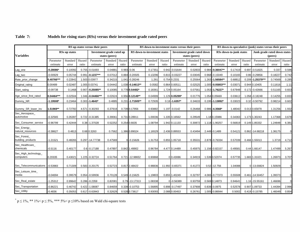
Table 7: Models for rising stars (RSs) versus their investment grade rated peers
Parameter estimate
Standard error
Hazard ratio
Parameter estimate
Standard error
Hazard ratio
Parameter estimate
Standard error
Hazard ratio
Parameter estimate
Standard error
Hazard ratio
Parameter estimate
Standard error
Hazard ratio
Parameter estimate
Standard error
Hazard ratio
Lag_one -0.28086* 0.10092 0.755 -0.01693 0.04881 0.983 -0.06 0.17351 0.942 -0.01644 0.02833 0.984 -0.36047** 0.17419 0.697 -0.51825 0.337 0.596
Lag_two -0.00929 0.05744 0.991 -0.1237*** 0.07012 0.884 -0.20505 0.13296 0.815 -0.03227 0.03045 0.968 -0.15049 0.10165 0.86 -0.29856 0.18227 0.742
Rate_prior_change 0.40766*** 0.22842 1.503 0.03977 0.34215 1.041 -0.28246 1.261 0.754 0.2331 0.25564 1.263 -1.56584** 0.68812 0.209 -1.25379*** 0.74569 0.285
Original_rating 0.00489 0.02487 1.005 0.03741 0.04442 1.038 -0.14613** 0.0582 0.864 0.00511 0.02525 1.005 -0.05803*** 0.03071 0.944 0.10405 0.11616 1.11
Start_rating -0.09738 0.1468 0.907 -0.25085** 0.10085 0.778 0.54482* 0.18361 1.724 0.05164 0.07561 1.053 -1.76227* 0.67848 0.172 -0.42666 0.51165 0.653
Age_since_first_rated 0.04464*** 0.02504 1.046 -0.04466*** 0.02624 0.956 0.12149** 0.04999 1.129 0.05299* 0.01776 1.054 0.05669 0.03612 1.058 -0.18248 0.14255 0.833
Dummy_NR -1.19508* 0.23464 0.303 -1.4643* 0.4885 0.231 -1.71505** 0.72935 0.18 -1.6357* 0.34633 0.195 -1.13892* 0.33023 0.32 -0.50792 0.98214 0.602
Dummy_SR_lower_inv 1.51969** 0.72782 4.571 -0.30293 0.37918 0.739 0.17956 0.93882 1.197 -0.0142 0.26468 0.986 -4.3568* 1.48042 0.013 0.65878 1.31256 1.932
Sec_Aerospace_ automotive -0.32565 0.35397 0.722 -0.31385 0.39061 0.731 0.28911 1.00036 1.335 0.16562 0.29549 1.18 0.15986 0.34363 1.173 1.30243 1.17368 3.678
Sec_Consumer_service -0.96799 0.42444 0.38 -1.37028 0.52252 0.254 0.6635 1.08794 1.942 0.11133 0.30872 1.118 -1.90257 0.56819 0.149 1.85332 1.24848 6.381
Sec_Energy_ natural_resources -0.38627 0.4813 0.68 0.3263 0.7562 1.386 0.89024 1.16529 2.436 0.89553 0.43494 2.449 -0.1489 0.54121 0.862 -14.68218 1.36175 0
Sec_Forest_ building_products -1.21521 0.48265 0.297 -14.77738 0.47569 0 -0.15626 1.31753 0.855 1.05718 0.35531 2.878 -0.76334 0.57039 0.466 1.55013 1.3719 4.712
Sec_Healthcare_ chemicals -0.5116 0.40177 0.6 -0.17188 0.47897 0.842 1.49902 0.96784 4.477 0.14489 0.45975 1.156 -0.82157 0.49581 0.44 1.66147 1.47499 5.267
Sec_High_technology_ computers 0.20335 0.43021 1.225 -0.32724 0.51764 0.721 -12.98652 0.90868 0 0.43086 0.34919 1.539 0.52074 0.57735 1.683 1.31021 1.26973 3.707
Sec_Telecommunications -0.53983 0.71309 0.583 -0.20175 0.52723 0.817 2.48422 0.98836 11.992 -0.65371 0.41272 0.52 -12.756 1.04088 0 -13.00824 1.50929 0
Sec_Leisure_time_ media -0.04694 0.39579 0.954 -0.59936 0.70128 0.549 -0.15625 1.19803 0.855 1.40249 0.32797 4.065 -0.77373 0.55508 0.461 -14.50457 1.39373 0
Sec_Real_estate -1.25312 0.99642 0.286 -0.2359 0.82081 0.79 -13.17313 1.08338 0 -0.56389 0.93759 0.569 0.14873 0.94641 1.16 -15.55161 1.46696 0
Sec_Transportation -0.86221 0.46742 0.422 -1.08087 0.84659 0.339 -0.10753 1.56895 0.898 -0.17497 0.37908 0.839 -0.0975 0.52578 0.907 1.09733 1.44394 2.996Sec_Utility -0.4836 0.35053 0.617 -0.63943 0.32629 0.528 0.73617 0.93093 2.088 0.00453 0.26761 1.005 -0.86944 0.5002 0.419 -0.15785 1.46049 0.854
RS up-states versus their peers RS down-to-speculative (junk) states versus their peersRS down-to-investment states versus their peers
* p ≤ 1%, ** 1%< p ≤ 5%, *** 5%< p ≤10% based on Wald chi-square tests
RS down-to-investment states Investment grade rated down states (peers)
RSs up states Investment grade rated up states (peers)
RSs down-to-junk states Junk grade rated down states (peers)Variables
Page 25
Table 8: Models for big rating jumpers versus their peers
Parameter estimate
Standard error
Hazard ratio
Parameter estimate
Standard error
Hazard ratio
Parameter estimate
Standard error
Hazard ratio
Parameter estimate
Standard error
Hazard ratio
Parameter estimate
Standard error
Hazard ratio
Parameter estimate
Standard error
Hazard ratio
Parameter estimate
Standard error
Hazard ratio
Parameter estimate
Standard error
Hazard ratio
Lag_one -0.10793* 0.033 0.898 -0.08043** 0.03227 0.923 -0.04512* 0.01608 0.956 -0.02447*** 0.0145 0.976 -0.02339 0.05294 0.977 -0.14186* 0.04157 0.868 0.03962 0.04347 1.04 -0.03823 0.03857 0.962
Lag_two -0.0008352 0.02394 0.999 -0.11108* 0.0328 0.895 0.02102 0.01393 1.021 -0.00411 0.01225 0.996 0.06236 0.03984 1.064 -0.08862** 0.0405 0.915 -0.08509*** 0.04614 0.918 -0.00595 0.03524 0.994
Rate_prior_change -0.03672 0.0842 0.964 -0.13816 0.18409 0.871 0.07686*** 0.04449 1.08 0.20495** 0.09706 1.227 0.1244 0.15139 1.132 0.27016 0.20211 1.31 0.19901 0.17244 1.22 0.41977 0.35554 1.522
Original_rating 0.07172* 0.01775 1.074 0.0739* 0.02619 1.077 -0.04064* 0.0103 0.96 -0.018 0.01352 0.982 0.03615** 0.01752 1.037 0.02498 0.02113 1.025 -0.06529* 0.01988 0.937 -0.02904 0.02467 0.971
Start_rating -0.19108* 0.02216 0.826 -0.21943* 0.02825 0.803 -0.09351* 0.01134 0.911 -0.0592* 0.01499 0.943 -0.1703* 0.02367 0.843 -0.18929* 0.02789 0.828 -0.03936*** 0.02449 0.961 -0.05559*** 0.03407 0.946
Age_since_first_rated -0.01809*** 0.01019 0.982 -0.0187 0.01359 0.981 0.01862* 0.00589 1.019 0.0131** 0.00649 1.013 -0.00564 0.0191 0.994 0.02873*** 0.01594 1.029 0.04246** 0.01652 1.043 0.05311** 0.01833 1.055
Dummy_NR -1.16724* 0.20619 0.311 -1.00592* 0.20231 0.366 -1.31963* 0.1301 0.267 -1.05178* 0.11934 0.349 -1.65149* 0.27054 0.192 -0.9755* 0.23743 0.377 -1.61443* 0.24376 0.199 -1.21731* 0.24014 0.296
Dummy_SR_junk_ boundary 0.61706* 0.15946 1.853 -0.04016 0.17058 0.961 -0.0415 0.10899 0.959 -0.2298** 0.1006 0.795 0.51548* 0.16115 1.674 0.49302* 0.15245 1.637 -0.55651* 0.20108 0.573 -0.49582** 0.24799 0.609
Dummy_SR_lower_inv 0.13571 0.17427 1.145 0.10449 0.14286 1.11 -0.2309** 0.09363 0.794 -0.10248 0.07864 0.903 0.87106* 0.2526 2.389 0.12476 0.18082 1.133 -0.5959** 0.25774 0.551 -0.35056*** 0.20773 0.704Dummy_junk_inv_ switch
NA NA NA NA NA NA NA NA NA NA NA NA-0.19443 0.2654 0.823 -0.07229 0.24425 0.93 0.41288 0.25853 1.511 -0.30885 0.31326 0.734
Dummy_inv_junk_switch -0.16111 0.17131 0.851 0.38583*** 0.22664 1.471 -0.29034** 0.11769 0.748 0.05189 0.15909 1.053 NA NA NA NA NA NA NA NA NA NA NA NA
Sec_Aerospace_ automotive 0.09115 0.21401 1.095 -0.36612 0.2369 0.693 -0.30014 0.1366 0.741 0.20767 0.13831 1.231 -0.09114 0.26236 0.913 -0.87063 0.24119 0.419 -0.50082 0.2546 0.606 0.2984 0.28271 1.348
Sec_Consumer_ service -0.02708 0.21695 0.973 -0.6047 0.23842 0.546 -0.08203 0.13385 0.921 0.15312 0.13096 1.165 -0.42595 0.30469 0.653 -0.94821 0.26341 0.387 -0.19782 0.25715 0.821 0.30369 0.28667 1.355
Sec_Energy_ natural_resources -0.18036 0.26735 0.835 -0.40663 0.30419 0.666 -0.27951 0.17947 0.756 -0.23622 0.17855 0.79 -0.33258 0.29284 0.717 -1.11884 0.29099 0.327 -0.96754 0.42382 0.38 -0.06017 0.44906 0.942
Sec_Forest_ building_products -0.31318 0.33489 0.731 -0.56651 0.27419 0.568 -0.3253 0.18975 0.722 -0.0779 0.16752 0.925 -0.47421 0.41012 0.622 -1.28099 0.28713 0.278 -0.47836 0.35708 0.62 0.05221 0.39028 1.054
Sec_Healthcare_ chemicals -0.05329 0.26137 0.948 -0.53184 0.2975 0.588 -0.22267 0.17473 0.8 -0.01783 0.1636 0.982 -0.32065 0.30954 0.726 -0.50834 0.2431 0.601 -0.49991 0.28191 0.607 0.05062 0.34756 1.052
Sec_High_technology_ computers 0.49757 0.28246 1.645 -0.43431 0.32968 0.648 -0.29478 0.17736 0.745 0.00188 0.19444 1.002 -0.22835 0.42582 0.796 -0.93793 0.35581 0.391 -0.10913 0.36992 0.897 -0.26249 0.48029 0.769
Sec_Telecommunications 0.33299 0.27202 1.395 -0.39723 0.35706 0.672 -0.00692 0.16086 0.993 0.12019 0.17935 1.128 -0.145 0.47675 0.865 -0.7662 0.27892 0.465 0.32266 0.28823 1.381 0.16231 0.33791 1.176
Sec_Leisure_time_ media -0.07349 0.24949 0.929 -0.4526 0.31467 0.636 -0.27992 0.15572 0.756 0.11208 0.16263 1.119 0.193 0.31721 1.213 -0.98075 0.25582 0.375 -0.08739 0.29731 0.916 0.34519 0.35532 1.412
Sec_Real_estate -0.902 0.63278 0.406 -0.94625 0.49208 0.388 -0.25332 0.23934 0.776 -0.19218 0.37579 0.825 -12.19581 0.61374 0 -0.98044 0.75861 0.375 -1.08523 1.17299 0.338 -12.35981 0.64561 0
Sec_Transportation -0.26847 0.23742 0.765 -0.71794 0.28743 0.488 -0.50005 0.16002 0.606 -0.12894 0.19023 0.879 0.0382 0.28538 1.039 -0.50925 0.39992 0.601 -0.87799 0.43696 0.416 -0.11037 0.56885 0.896Sec_Utility 0.24554 0.2059 1.278 -0.12869 0.20774 0.879 -0.19551 0.13969 0.822 -0.28921 0.1348 0.749 0.03156 0.25294 1.032 -0.69732 0.19119 0.498 -0.50594 0.25364 0.603 -0.0712 0.26341 0.931
^^^ Big-up-jump up states are up states with the non-censored immediate prior rating state underwent an up jump of at least 2 notches (dummy_big_jump_up=1). Their peers are up states with the non-censored immediate prior rating state experienced an upgrade of 1 notch (dummy_lag_up=1 and dummy_big_jump_up=0)^^^^ Big-up-jump down states are down states with the non-censored immediate prior rating state underwent an up jump of at least 2 notches (dummy_big_jump_up=1). Their peers are down states with the non-censored immediate prior rating state experienced an upgrade of 1 notch (dummy_lag_up=1 and dummy_big_jump_up=0)
Big-down-jump Up-states Lag-one-down up-states (peers)
Big-up-jump up-states Lag-one-up Up states (peers)
* p ≤ 1%, ** 1%< p ≤ 5%, *** 5%< p ≤10% based on Wald chi-square tests
Big-up- jump Down-states Lag-one-up Down-states (peers)
^ Big-down-jump up states are up states with the non-censored immediate prior rating state underwent a down jump of at least 2 notches (dummy_big_jump_down=1). Their peers are up states with the non-censored immediate prior rating state experienced a downgrade of 1 notch (dummy_lag_down =1 and dummy_big_jump_down=0)
Down states with a lag one big up jump vs. their peers^^^^
Big-down- jump Down-states Lag-one-down down-states (peers)
^^ Big-down-jump down states are down states with the non-censored immediate prior rating state underwent a down jump of at least 2 notches (dummy_big_jump_down=1). Their peers are down states with the non-censored immediate prior rating state experienced a downgrade of 1 notch (dummy_lag_down =1 and dummy_big_jump_down=0)
Variables
Up states with a lag one big down jump vs. their peers^ Down states with a lag one big down jump vs. their peers^^ Up states with a lag one big up jump vs. their peers^^^
Page 26
Figure 1Histogram of the length of fallen angel down-states, 1982-2005
Histogram of the length of fallen angel up-to-junk states, 1982-2005
Histogram of the length of fallen angel up-to-investment states, 1982-2005
Histogram of the length of rising star up-states, 1982-2005
Histogram of the length of rising star down-to-junk states, 1982-2005
Histogram of the length of rising star down-to-investment states, 1982-2005
Page 27
Figure 2
Histogram of the length of big-down-jump down-states, 1982-2005
Histogram of the length of big-down-jump up-states, 1982-2005
Histogram of the length of big-up-jump down-states, 1982-2005
Histogram of the length of big-up-jump up-states, 1982-2005