Ratio Analysis and Equity Valuation From Research to Practice.

Review of Accounting Studies, 6. I()9-154, 20012001 KJuwer Academic Publishers. Manufactured in The Netherlands.

Ratio Analysis and Equity Valuation:From Research to Practice

DORON NlSSIM [email protected] University, Graduate School of Business. 3022 Broadway. Uris Halt 604. New York. NY 10027

STEPHEN H. PENMAN [email protected] University. Graduate School of Business. 3022 Broadway, Uris Hall 612, New York. NY 10027

Abstract. Financial statement analysis has traditionally been seen as part of the fundamental analysis requiredfor equity valuation. But the analysis has typically been ad hoc. Drawing on recent research on accounting-basedvaluation, this paper outlines a financial .statement analysis for use in equity valuation. Standard proHtabilityanalysis is incorporated, and extended, and is complemented with an analysis of growth. An analysis of operatingactivities is distinguished from the analysis of financing activities. The perspective is one of forecasting payoffsto equities. So financial statement analysis is presented as. a matter of pro forma analysis of the future, witbforecasted ratios viewed as building block.s of forecasts of payoffs. The analysis of curtent financial statements isthen seen a.s a matter of identifying curTeni ratio.s as predictors of the future ratios that determine equity payoffs.The financial statement analysis is hierarchical, with ratios lower in the ordering identified as finer informatiotiabout those higher up. To provide historical benchmarks for forecasting, typical values for ratios are documentedfor the period 1963-1999, along with their cross-sectional variation and correlation. And. again with a view toforecasting, the time series behavior of many of the ratios is also described and their typical "long-run, steady-state"levels are documented.

Keywords: Financial statement analysis, ratio analysis, equity valuation

It goes almost without saying that, in an applied discipline like accounting, the aim ofresearch is to affect practice. Theory can be admired on a ntmiber of dimensions, but a streamof research is ultimately judged on the products it delivers, how it enhances technology.Engineering and medical research, to name just two endeavors, have this orientation. Ourcolleagues in finance have been successful in product development. While making majorcontributions to economic theory, they have also engineered such products as derivativepricing, risk measurement, hedging instruments, portfolio insurance, and asset allocation,some, to be sure, more successful than others.

In the area of equity analysis, research in finance has not been successful. Equity analysis—or fundamental analysis—was once the mainstream of finance. But, while enormous stepshave been taken in pricing derivatives on the equity, techniques to value equities have notadvanced much beyond applying the dividend discount model. So-called asset pricing mod-els, like the Capital Asset Pricing Model, have been developed, but these are models of riskand the expected return, not models that instruct how to value equities. Real option anal-ysis has been applied to equity valuation, but the measurement problems are significant.Some progress has been made by accounting researchers in what has come to be referredto as accounting-based valuation research. That is not surprising. Equity analysis is largelyan analysis of information, and accountants deal with infonnation about firms. This papercarries the recent research to the level of product design.

110 NlSSIM AND PENMAN

Traditional fundamental analysis (before modem finance) was very much grounded in thefinancial statements. So, for example, Graham, Dodd and Cottle's5ecwr(f\'Arta/v5i5(1962)is not the security analysis of modem finance texts (that involves the analysis of prices, betaestimation, and asset allocation), but rather security analysis that analyzes fundamentalsthrough the financial statements. However, financial statement measures were linked toequity value in an ad hoc way, so little guidance was given for understanding the implicationsof a particular ratio—a profit margin or an inventory tumover, for example—for equity value.Nor was a comprehensive scheme advanced for "identifying, analyzing and summarizing"financial statement information in order to draw a conclusion as to what the statements, asa whole, say about equity value. Equity value is determined by "future eamings power,"it was said, but there was no explicit justification for using future eamings as a valuationattribute, nor was there explicit development of the forecasting of this eamings power.

A considerable amount of accounting research in the years since Graham, Dodd andCottle has been involved in discovering how financial statements inform about equity value.The whole endeavor of "capital markets research" deals with the "information content" offinancial statements for determining stock prices. The extensive "time-series-of-eamings"literature summarized in Brown (1993) focuses on forecasting eamings, often with valuationin mind. Papers such as Lipe (1986), Ou (1990), Ou and Penman (1989), Lev and Thiagarajan(1993) and Fairfield, Sweeney and Yohn (1996), to name just a few, have examined the roleof particular financial statement components and ratios in forecasting. But it is fair to saythat the research has been conducted without much structure. Nor has it produced manyinnovations for practice. Interesting, robust empirical correlations have been documented,but the research has not produced a convincing financial statement analysis for equityvaluation. Indeed the standard textbook schemes for analyzing statements, such as theDuPont scheme, rarely appear in the research.

Drawing on recent research on accounting-based valuation, this paper ventures to producea stmctural approach to financial statement analysis for equity valuation. The structure notonly identifies relevant ratios, but also provides a way of organizing the analysis task. Theresult is a fundamental analysis that is very much grounded in the financial statements;indeed, fundamental analysis is cast as a matter of appropriate financial statement analysis.The structural approach contrasts to the purely empirical approach in Ou and Penman(1989). That paper identified ratios that predicted eamings changes in the data: no thoughtwas given to the identification. The approach also contrasts to that in Lev and Thiagarajan(1993) who defer to "expert judgment" and identify ratios that analysts actually use inpractice.

Valuation involves forecasting payoffs. Forecasting is guided by an equity valuation modelthat specifies what is to be forecasted. So, for example, the dividend discount model directsthe analyst to forecast dividends. Because it focuses on accrual-accounting financial state-ments, the residual income valuation model, recently revived through the work of Ohlson(1995) and Feltham and Ohlson (1995), serves as an analytical device to organize thinkingabout forecasting and analyzing financial statements for forecasting. This model is a state-ment of how book value and forecasted eamings relate to forecasted dividends and thusto value. The ratio analysis in this paper follows from recognition of standard accountingrelations that determine how components of the financial statements relate to eamings andbook values.

RATIO ANALYSIS AND EQUITY VALUATION 1 1 1

Our focus on the residual income valuation model is not to suggest that this model is theonly model, or even the best model, to value equities. Penman (1997) shows that dividendand cash-flow approaches give the same valuation as the residual income approach undercertain conditions. The residual income model, based as it is on accrual accounting, isof particular help in developing an analysis of accrual-accounting financial statements.But cash flows and dividends are tied to accrual numbers by straightforward accountingrelations, so building forecasts of accrual accounting numbers with the aid of analysis buildsforecasts of free cash flows and dividends also, as will be seen.

The scheme is not offered as the definitive way of going about financial statement analysis.There is some judgment as to "what makes sense." Tbis is inevitably part of the art of designin bringing academic models to practice (Colander (1992)). As such it stands as a point ofdeparture for those wiih better judgment.

The paper comes in two parts. First it identifies ratios that are useful for valuation. Second,it documents typical values of the ratios during the period 1963 to 1999.

Identification. Residual earnings valuation techniques are so-called because equity valueis determined by forecasting residual income. As a matter of first order, ratio identificationamounts to identifying ratios that determine—or drive—future residual income so that, byforecasting these ratios, the analyst builds a forecast of residual income. So relevant ratiosare identified as the building blocks of a forecast, that is, as the attributes to be forecastedin order to build up a forecast of residual income. However, ratios are usually seen asinformation in current financial statements that forecasts the future. So cunent financialstatement ratios are deemed relevant for valuation if they predict future ratios. Accordinglythe identification of (future) residual income drivers is overlaid here with a distinctionbetween "transitory" features of ratios (that bear only on the present) and "permanent"features (that forecast the future).

At the core is an analysis of profitability. Many of the standard profitability ratios areincluded, so many aspects of the analyses are familiar. Indeed the paper serves to inte-grate profitability analysis witb valuation. But refined measures of operational profitabilityare presented and an alternative analysis of leverage is introduced. And profitability ratiosare complemented with ratios that analyze growth, for both profitability and growth driveresidual earnings.

Not only are relevant ratios identified, but an algebra—like the traditional DuPont analysis(which is incorporated here)—ties the ratios together in a structured way. This algebra notonly explains how ratios "sum up" as building blocks of residual income but also establishesa hierarchy so that many ratios are identified as finer information about others. So the analystidentifies certain ratios as primary and considers other ratios down the hierarchy only iftbey provide further information. This brings an element of parsimony to practical analysis.But it also provides a structure to researchers who wish to build (parsimonious) forecastingmodels and accounting-based valuation models.

In residual income valuation, forecasted income must be comprehensive income, other-wise value is omitted. So the ratio analysis is based on a comprebensive income statement.This is timely because FASB Statement No. 130 now requires the reporting of compre-hensive income on a more transparent basis, and other recent FASB statements, notablystatements 115 and 133, have introduced new components of comprehensive income. But

112 NISSIM AND PENMAN

comprehensive income contains both permanent and transitory components of income. Forforecast and valuation, these need to be distinguished.

The analysis makes a separation between operating and financing items in the financialstatements. This is inspired by the Modigliani and Miller notion that it is the operatingactivities that generate value, and that apart from possible tax effects, the financing activitiesare zero net-present-value activities. The separation also arises from an appreciation thatfinancial assets and liabilities are typically close to market value in the balance sheet (moreso since FASB Statement No. 115) and thus are already valued. But not so for the operatingassets and liabilities, so it is the operating activities that need to be analyzed. The distinctionis a feature ofthe accounting-based valuation model in Feltham and Ohlson (1995) and of"economic profit" versions ofthe residual income model.

The distinction between operating and financing activities requires a careful separation ofoperating and financing items in the financial statement that leads, in the paper, to a refinedmeasure of operating profitability to the one often advanced in texts, it also leads to betterunderstanding of balance-sheet leverage that involves two leverage measures, one arisingfrom financing activities, the other from operating activities. And it isolates growth as anattribute of the operating activities, not the financing activities, and develops measures ofgrowth from the analysis ofthe operating activities.

Documentation. Ratio analysis usually compares ratios for individual firms against bench-marks from comparable firms—both in the past and the present—to get a sense of what is"normal" and what is "abnormal." The paper provides a historical analysis of ratios thatyields such benchmarks for the equity researcher using residual earnings techniques.

Appreciating what is typical is of assistance in developing prior beliefs for any forecasting,and particularly so in a valuation context because there is a tendency for many ofthe relevantratios to revert to typical values over time, as will be seen. Further, valuation methods thatinvolve forecasting require continuing value calculations at the end of a forecast period.These calculations require an assessment of a "steady state" for residual income and areoften seen as problematical. The documentation here gives a sense of ibe typical steady statefor the drivers of residual income and thus a sense of the typical terminal value calculationsrequired. It shows that steady-state conditions typically occur within "reasonable" forecasthorizons and their form is similar to that prescribed by residual income models. This givesa level of comfort to those applying residual income techniques.

The documentation also helps in the classification of financial statement items into"permanent" and "transitory." This classification inevitably involves some judgment butthe displays here give typical "fade rates" for the components of residual income driversand thus an indication of which components are typically transitory.

1. The Residua] Earnings Valuation Model

There are many ratios that can be calculated from the financial statements and the equityanalyst has to identify those that are important. The residual earnings equity valuation modelbrings focus to the task-

The residual earnings model restates the non-controversial dividend discount model. Rec-ognizing the (clean surplus) relation that net dividends are always equal to comprehensive

RATIO ANALYSIS AND EQUITY VALUATION 113

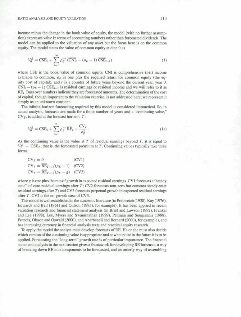
income minus the change in the book value of equity, the model (with no further assump-tion) expresses value in terms of accounting numbers rather than forecasted dividends. Themodel can be applied to the valuation of any asset but the focus here is on the conmionequity. The model states the value of common equity at date 0 as

Vo = CSEo -f J2PE' (CNT, -{pE-\) CSE,_i) (1)i=i

where CSE is the book value of common equity, CNI is comprehensive (net) incomeavailable to common, p£ is one plus the required return for common equity (the eq-uity cost of capital), and r is a counter of future years beyond Ihe current year, year 0.CNI, — (pf — 1) CSEj_i is residual earnings or residual income and we will refer to it asR£,. Bars over numbers indicate they are forecasted amounts. The determination ofthe costof capital, though important to the valuation exercise, is not addressed here; we represent itsimply as an unknown constant.

The infinite-horizon forecasting required by this model is considered impractical. So, inactual analysis, forecasts are made for a finite number of years and a "continuing value,"CVj-, is added at the forecast horizon, T:

V^ = CSEo + Y.P-E RE, -h . (U)t=\ PE

As the continuing value is the value at T of residual earnings beyond T, it is equal toVj — CSEr, that is, the forecasted premium al T. Contintiing values typically take threeforms:

= 0 (CVI)

= ^ 7 - n / ( P E - l ) {CV2)

CVr = REr+i / (PE-g) (CV3)

where g is one plus the rate of growth in expected residual earnings. CVI forecasts a "steadystate" of zero residual earnings after 7"; CV2 forecasts non-zero but constant steady-stateresidual earnings after T\ and CV3 forecasts perpetual growth in expected residual earningsafter T. CV2 is the no-growth case of CV3.

This model is well established in the academic literature (in Preinreich (1938). Kay (1976),Edwards and Bell (1961) and Ohlson (1995). for example). It has been applied in recentvaluation research and financial statement analysis (in Brief and Lawson (1992), Frankeland Lee (1998), Lee, Myers and Swaminathan (1999), Penman and Sougiannis (1998),Francis, Olsson and Oswald (2000), and Abarbanell and Bernard (2000), for example), andhas increasing currency in financial analysis texts and practical equity research.

To apply the model the analyst must develop forecasts of RE. He or she must also decidewhich version of the continuing value is appropriate and at what pwint in the future it is to beapplied. Forecasting the "long-term" growth rate is of particular importance. The financialstatement analysis in the next section gives a framework for developing RE forecasts, a wayof breaking down RE into components to be forecasted, and an orderly way of assembling


mformation to forecast these components. The documentation in Section 3 gives historicalvalues for the components and evidence on steady state for RE and its components.

2. Ratio Identification

Residual earnings compares earnings to net assets employed and so is a measure of prof-itability. Residual earnings can be expressed in ratio form as:

RE, = [ROCE, - {pE - l)]CSE,_i

where ROCE, = CNl,/CSE,_i is the rate of retum on common equity. So forecastingresidual earnings involves forecasting ROCE and book values to be put in place to eamthe forecasted ROCE. Distinguishing ROCE and book value as two separate attributes toforecast helps to compartmentalize the task. But this is not to mean that return on bookvalues and book values are independent. Formally, while this expression holds for realizedreturns, it is not the case that

_,] = \E ( ^ ^ ) - (PE - 1)

unless CNI,/CSE,_i and CSE,_-| are uncorrelated. The amount of equity investment mightdepend on ROCE and the accounting for book values may affect ROCE. Under conservativeaccounting, for example. ROCE is below its no-growth rate if investments are growing, andreducing investments generates higher ROCE, as modeled in Beaver and Ryan (2000) andZhang (2000). Strictly, the forecast is of expected book values and expected earnings onexpected book values. Accordingly, forecasting is done as a matter of scenario analysis:ROCE and book values are forecasted for alternative scenarios, producing forecasted C Mand CSE for each scenario, then averages are taken over probability-weighted scenarios.So tbe analysis here should be seen as one for developing forecast scenarios.' Contingentscenarios can be incorporated .so that scenarios involving "real options," growth options andadaptation options are thus accommodated by the analysis.

2.1. The Drivers of Retum on Common Equity (ROCE)

ROCE is the summary profitability ratio in financial statements and is "driven" by in-come statement line items that sum to net income in the numerator and balance sheetitems that sum to the net assets in the denominator. Residual income valuation requiresthat forecasted income be comprehensive income, otherwise value is lost. So our incomestatement analysis is of all the line items that sum to comprehensive income. Our analy-sis also distinguishes operating profitability from the profitability identified with the fi-nancing activities. As is standard, operating activities are those involved in producinggoods and services for customers. Financing activities have to do with raising cash forthe operations and disposing of cash from the operations.^ A division of line items thatdistinguishes operating from financial activities is a starting point for analysis of ROCE


drivers:

CNl = Comprehensive Operating Income (01)

— Comprehensive Net Financial Expense (NFE) (2)

CSE = Net Operating Assets (NOA) - Net Financial Obligations (NFO) (3)

where

NFE = (Financial Expense — Financial Income), aftertax

NOA = Operating Assets (OA) - Operating Liabilities (OL)

NFO = Financial Obligations (FO) — Financial Assets (FA).

Operating liabilities are those generated by operations (like accounts payable, wages pay-able, pension liabilities and deferred tax liabilities), while financiai liabilities are those fromraising funds to finance operations. Financiai assets (bonds held) are available to financeoperations and effectively reduce debt to finance operations (bonds issued). Balance sheettotals are maintained; that is.

Total Assets = OA -H FA,

Total Liabilities & Preferred Stock - OL + FO,

so all balance sheet items are assigned to a category.Net financial expense (NFE) is the (comprehensive) net expense flowing from net financial

obligations and includes interest expense minus interest income, preferred dividends, andrealized and unrealized gains and losses on financial assets and obligations; all items drawingtax or tax benefits are multiplied by (1 — marginal tax rate) unless reported on an after-taxbasis. All accounting item.s are identified from tbe common shareholders' point of view.Thus preferred dividends are a financial expense and preferred stock is a financial obligation.If a firm has net financial assets rather than net financial obligations (financial assets aregreater than financial obligations) then it generates net financial income rather than netfinancial expense.

Operating income (01 = CNI + NFE) is the income flowing from net operating assetsand, by the calculations here, is after tax.

Comparing each income statement component to its corresponding balance sheet com-ponent yields measures of operating profitability and financing profitability:

01,Retum on Net Operating Assets (RNOA), = NOA,_i

and

NFENet Borrowing Cost (NBC), = ' .

RNOA is different from the more common retum on assets. Retum on assets include financialassets in its base and excludes operating liabilities, so it confuses operating and financing


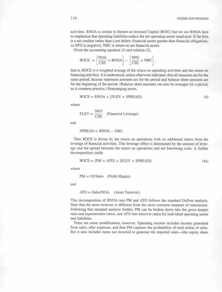
activities. RNOA is similar to Return on Invested Capital (ROIC) but we use RNOA hereto emphasize that operating liabilities reduce the net operating assets employed. If the firmis a net creditor rather than a net debtor (financial assets greater than financial obligations,so NFO is negative), NBC is return on net financial assets.

Given the accounting equation (3) and relation (2),

that is, ROCE is a weighted average of the return on operating activities and the return onfinancing activities. It is understood, unless otherwise indicated, that all measures are for thesame pedod. Income statement amounts are for the period and balance sheet amounts arefor the beginning of the period. (Balance sheet amounts can also be averages for a period,as is common practice.) Rearranging terms,

ROCE = RNOA -I- [FLEV x SPREAD] (4)

where

FLEV = (Financial Leverage)CSE

and

SPREAD = RNOA - NBC.

Thus ROCE is driven by the return on operations with an additional return from theleverage of financial activities. This leverage effect is determined by the amount of lever-age and the spread between the return on operations and net borrowing costs. A furtherdecomposition yields

ROCE = [PM X ATO] + [FLEV x SPREAD] (4a)

where

PM = Ol/Sales (Profit Margin) •

and

ATO = Sales/NOA. (Asset Tumover)

This decomposition of RNOA into PM and ATO follows the standard DuPont analysis.Note that the asset tumover is different from the more common measure of sales/assets.Following that standard analysis further, PM can be broken down into the gross marginratio and expense/sales ratios, and ATO into tumover ratios for individual operating assetsand liabilities.

There are some modifications, however. Operating income includes income generatedfrom sales, after expenses, and thus PM captures the profitability of each dollar of sales.But it also includes items not incurred to generate the reported sales—like equity share


of income in a subsidiary, dividends, and gains and losses on equity investments markedto market. We refer to these items as Other Items and exclude them from a revised profitmargin:

Sales PM = 01 from Sales/Sales.

So.

ROCE = [Sales PM x ATO] 4- ' ^ ^ ^ J ^ ^ ' " ^ + [FLEV x SPREAD]. (5)NOA

Both Sales PM and Other Items are after tax. Other Items/NOA has Uttle meaning, but"profitability of sales" is identified without noise. Profit margins are typically regarded ascrucial and this revised profit margin cannot be affected by acquisitions accounted for underthe equity method (for example).

A further modification is required when there are minority interests in subsidiaries, forminority interests share with the common shareholders in earnings. With minority interests(MI) on the consolidated balance sheet, equation (3) is restated to

CSE = NOA - NFO - MI.

And retum on total common equity is calculated as

ROTCE = (CNl + MI share of income)/(CSE + MI).

The components in (5), with FLEV redefined as NFO/(CSE + MI), aggregate to ROTCBrather than ROCE and

ROCE = ROTCE x MSR (6)

where

CNI/(CNI + Ml share of income)Minority Sharing Ratio (MSR) =

CSE/(CSE + Ml on balance sheet)'

An additional driver of RNOA involves operating liabilities. Clearly the netting out ofoperating liabilities in the calculation of NOA increases RNOA through a denominatoreffect, and appropriately so: to the extent that a firm has "non-interest" credit from payables(for example) it levers up its RNOA. This leverage is a driver of profitabihty that is distinctfrom financial leverage, for it arises in the operations, not the financial activities.^ Thisleverage can be analyzed. Suppliers who advance the payables reduce the net investmentrequired to run the operations and so lever up the operating profitability, but supplierspresumably charge implicitly for the credit in terms of higher prices. Denote io as theimplicit interest charge on operating liabihties other than undiscounted deferred taxes, andcalculate

OA


as the Retum on Operating Assets that would be made without leverage from operatingliabilities. Then

RNOA = X — — - —- X - - — = ROOA + [OLLEV x OLSPREAD]OA 1 r io OL 1 _

NOAJ ~ [OL ^ NOAJ(7)

where

OLOLLEV =

NOA

is operating liability leverage, and

OLSPREAD = ROOA - —OL

is operating liability spread. This is of the same form as the financial leverage formula in(4): RNOA is levered up by operating liability leverage and the leverage effect is deter-mined by the operating liability leverage and the spread between ROOA and the implicitborrowing cost. The implicit borrowing cost can be estimated with the short-term borrowingrate."" Like financial leverage, the analysis shows that operating liability leverage can befavorable or unfavorable; the leverage is favorable only if ROOA is greater than the implicitborrowing cost.

This analysis yields seven drivers of ROCE:

• Sales Profit Margin (Sales PM)

• Asset Tumover (ATO)

• Other Items/NOA

• Financiai Leverage (FLBV)

• Net Borrowing Cost (NBC) which, when compared to RNOA. gives SPREAD

• Operating Liability Leverage (OLLEV)

• Minority Interest Sharing (MSR)

Forecasting ROCE involves forecasting these drivers and aggregating them according to(5) (with ROTCE substituted for ROCE), (6) and (7).

2.2. The Drivers of Book Value

To forecast residual income one must forecast CSE as well as ROCE. CSE can be decom-posed into

^^^ o . NOA CSECSE = Sales x x

Sales NOA


and thus, when there are no minority interests,

CSE = Sales x x . (8)ATO 1 -I- FLEV ^ '

Sales drive the net operating assets and 1 /ATO is the amount of NOA that has to be pul inplace to generate a dollar of sales. The NOA can be financed by equity or borrowing and1/(1 -j- FLEV) captures this financing decision. Accordingly, future CSE is forecasted bypredicting three drivers:

• Sales

• Asset Turnover (ATO)

• Financial Leverage ^

With the forecast of the drivers in (5), (6), (7) and (8), the forecasting of residual earningsis complete. The nesting of ratios within (5), (6), (7) and (8)—so that they "aggregate"—•is by careful definition and accounting relations (2) and (3), and involve no economicassumptions. The relationships hold under all economic conditions and for all accountingprinciples provided earnings are comprehensive earnings.

2.3. Reducing the Analysis

Just as residual earnings can be calculated for common equity (net assets) so it can be cal-culated for any component of net assets. For the two (operating and financing) componentsidentified above.

Residual Operating Income (ReOI), = 01, — (p^. — 1) NOA,_i

and

Residual Net Financial Expense (ReNFE), = NFE, - {po - 1) NFO,_|

Pu) is the required return for the operations (we use "w" to donate it as the weighted-averagecost of capital, as is standard) and po the required return on the net financial obligations(the cost of capital for debt). The value of the net operating asset component of equity is

1=1

This is often referred to as the value of the firm or enterprise value. The value of the netfinancial obligations is

= NFOo +r= l


By the accounting equation (applied to values rather than book values).

and so V(f as stated in (1) is equivalent to*

Vo = NOAo - NFOo + 2^ Pw ReOI< - 2 ^ PD ReNFE,.f=i r - l

For any asset or obligation measured at market value, forecasted residual income mustbe equal to zero (it is forecasted to earn at the cost of capital). If NFO is measured on thebalance sheet at market value such that NFO = Vy ", then the present value of forecastedReNFE, is zero (and if the present value of ReNFE is zero, then NFO = Vj^"'^). If so, thenfor finite forecast horizons,

^ cyv,^ = csEo + ypr

(=1 ^

with three forms for the continuing value:

= 0 (CVOl)

^ ^ k l i (CV02)pw - 1

Pw -8

where g is now one plus the forecasted growth rate in ReOI beyond T.Residual operating income, like residual income, can be expressed in terms of a ratio

measure of profitability:

ReOI, = [RNOA, - (/)w - 1)] NOA,_|

so ReOI is forecasted by predicting RNOA and the net operating assets to be put in place toearn at the forecasted RNOA. Again, operating income and NOA may not be independentso the analysis applies to scenarios. Accordingly, with a valuation based on forecastingReOI, the number of drivers to be predicted are reduced. The drivers of RNOA are

• Sales Profit Margin (Sales PM)


• Other Items/NOA

• Operating Liability Leverage (OLLEV)

As NOA = Sales/ATO, the drivers of NOA are

• Sales



This reduction in the forecasting task is a clear efficiency. Financial leverage considera-tions drop out, including leverage effects on the cost of capital. One needs only forecast theoperating profitability and the NOA and forget forecasting borrowing and dividend policy.But the approach is only appropriate if financial assets and financial obligations are mea-sured at their fair value. This is the case for many financial assets under FASB StatementNo. 115. Other financial assets and liabilities are often close to market value (as a work-able approximation), or their fair values are disclosed in footnotes under FASB StatementNo. 107.

RNOA and NOA have a common driver (ATO). ReOI can be detennined in one step thatutilizes both RNOA and NOA drivers:

ReOI = Sales x [pM - ^ " ' ~ ' 1 (10)

The ratio, (pw — 1)/ATO compares the ATO to the required retum on operations and isa measure of the efficiency of the NOA in generating sales relative to the required returnon NOA.

2.4. The Drivers of Growih in Residual Earnings

Growth is an important aspect of valuation, particularly for the calculation of continuingvalues. With residual income valuation, the appropriate growth concept is growth in expectedresidual earnings.' Since residual income, for a given scenario, is driven by the accountingrate of retum and book value, its growth is driven by increases in the rale of retum and/orincreases in book value. There are simplified calculations to capture this. We deal withresidual operating income, with the calculation for full residual income implicit. The growthrate is

Growth Rate in ReOI, = ReOWReOI,_. - 1 = [ ^ Q A . ^w + 1]NOA,_. _[RNOA,_, -pw + 1]NOA

So growth in ReOI (which can be greater or less than 0) is driven by changes in RNOA,NOA, and the cost of capital. We deal witb cases where the forecasted cost of capital isconstant.

Constant RNOA

Pro forma analysis often comes to the conclusion that, in "the long-run," profitability willconverge to a permanent level. If this is such that, at a point, T, in the future, one forecaststhat subsequent RNOA will equal the cost of capital, then expected ReOI is zero. But if oneforecasts that RNOA will be different from the cost of capital but constant, then

Growth Rate in ReOI, = — - 1N0A

for all / > T. Growth is driven solely by increases in NOA.

122 . ^4IS5IM AND PENMAN

A permanent level of non-zero ReOI (RNOA ^ cost of capital) may reflect permanentabnormal real profitability (in the sense tbat the firm can invest always in non-zero net presentvalue projects). But it can also be induced by the accounting: conservative accounting, forexample, that always keeps book values low (by expensing R&D, for example) will yieldpermanent positive ReOI even with zero NPV projects. This is modeled in Feltham andOhlson (1995). Beaver and Ryan (2000) provide some empirical evidence.

Constant RNOA, Constant PM and Constant ATO

As RNOA is driven by profit margin and tumover, a constant RNOA can be driven bya changing PM with a canceling effect of changing ATO, and by both constant PM andconstant ATO. In the latter case growth in ReOI is driven solely by growth in sales. From(10), growth in ReOI can also be expressed as

Sales, X [pM, - ^ ^Growth Rate in ReOI, = f ^-5__ - 1

Salesj-i X PM,_i —

thus, for constant PM and ATO (and cost of capital),

„ . . Sales,Growth Rate in ReOI, = • 1.

Sales, _i

A constant PM and ATO means constant RNOA and growth in ReOI detennined only bygrowth in NOA. But a constant ATO means NOA grows at the same rate as sales. One needonly forecast sales growth to get the growth rate.

Varying RNOA and Constant NOA

In this case growth in ReOI is driven by changes in RNOA. One would expect it to applyin the case of declining RNOA, not increasing RNOA. RNOA and growth in NOA arepresumably not independent. So. for example, increasing RNOA might generate moreinvestment in NOA, declining RNOA less investment in NOA.

2.S. The Drivers of Free Cash Flow and Dividends

Comprehensive income is defined sucb that for a period, /,

CSE, = CSE,^, -H CNI, - d,

where d, is net dividends (dividends 4- share repurchases — share issues). So, recognizingthe division of comprehensive income into operating and financing components in (2) and


the accounting equation in (3),

NOA, - NFO, = NOA,_| - NFO,_i + 01, - NFE, - d,. (11)

Free cash flow, = C, — /, where C, is cash flow from operations and /, is cash flow ininvesting activities. Under accrual accounting, operating income modifies free cash flowfor investment and accruals:

OI, = C, — /, + / , + Operating Accruals/,

and net operating assets are recorded hy placing the adjustments to free cash flow in thebalance sheet:

ANOA, = /, + Operating Accruals; = OI, - (C, - /,) (12)

where A indicates change (growth). As, from (11), the change in NOA is also

ANOA, = ANFO, + 01, - NFE, - d^,

then

ANFO, =d,+ NFE, - (C, - I,). (13)

Rearranging the difference equations (12) and (13),

Q-J,=^ 01; - ANOA, = NOA,_i [RNOA, -

and

d, = C,~I,- NFE, + ANFO,. (15)

We have developed the ratio analysis with residual income valuation in mind. But it isclear from (14) that the same drivers that drive ReOI—RNOA and NOA growth—alsodrive free cash flow, so the ratio analysis also applies to discounted cash flow analysis.Forecasting free cash flows requires no additional information once RNOA and growth inNOA are forecasted, as (14) is just an accounting relation. And indeed one cannot imagineforecasting free cash flow without first forecasting profltahility and the investment in NOAthat drive free cash flow.^

If dividend discounting techniques are used to value equity. (15) shows that dividends arealso forecasted from forecasts of free cash flow drivers, along with a forecast of financingactivities: dividends are the residual of free cash flow after servicing net debt.

2.6. Forecasting and the Analysis of Current Financial Statements

The drivers identified generate both current and future rates of return and book values. Thefuture drivers are the building blocks of forecasted residual earnings. Drivers are identified


in current financial statements to forecast future drivers. Accordingly, the analysis of currentfinancial statements should be guided by the "predictive ability" criterion: any enhancementthat improves forecasts is an innovation.

This perspective calls for an analysis that distinguishes aspects of the drivers that willlikely drive the future ("persistent" features) and those that relate only to the present ("tran-sitory" features). And some features may persist for a short period (transitory but not puretransitory) while some may be enduring ("permanent" features). This distinction is partic-ularly important for the analysis of comprehensive income (which is required for residualincome valuation), as comprehensive income below "net income" under FASB StatementNo. 130 typically includes a number of transitory items.

We will refer to items judged persistent as "core items" and those judged transitory as"unusual items." So

01 = Core OI + Unusual Operating Income (UOI)

and

NFE = Core NFE + Unusual Financial Expense (UFE).

Tax is allocated to these components unless they are reported net of tax. With this division.

Core 01 from Sales Core other Items UOI

+ +NOA NOA NOA

Similarly,

UFE are transitory components from realized and unrealized gains and losses on financialitems and Core NBC is the borrowing cost (cost of debt capital) minus interest yield onfinancial assets.

The distinction between core and unusual items and sales and non-sales items can be usedto further decompose ROCE. Calculate

^ „ , , Core 01 from SalesCore Sales PM =

Sales

and substitute in (5):

ROCE = [Core Sales PM x ATO] + ^ ° " ? . ^ " ^ ^ ^ " ^ +NOA NOA

FLEV X I Core RNOA - Core NBC -

Core RNOA - Core NBC is the Core SPREAD. But, if one is forecasting ReOI and valuingaccording to (9), only the RNOA decomposition is relevant. Indeed, the dismissal of financial


items from the valuation in (9) can he justified on the grounds that any deviation of currentNBC from the cost of capital for debt (like gains and losses on financial items) is puretransitory and does not affect the forecast of future residual income (or expense) fromfinancing activities.^

Expression (16) does not incorporate all the drivers that have been identified. This can bedone as follows:

ROCE = MSR X [(Core Sales PM* x ATO') + C°re Other Items ^ UOI[ OA OA

-I- (OLLEV X OLSPREAD) -I- (FLEV x SPREAD)

where Core Sales PM' = (Core 01 from Sales -H io)/Sales, ATO* = Sales/OA, FLEV =NFO/(CSE + MI) and the SPREAD is decomposed as in (16). This includes the MinoritySharing Ratio (MSR) and the operating liability leverage drivers. But it revises the assettumover to ATO* which excludes operating liabilities.

Focusing on ReOI and the operating activities, an item is classified as unusual if it isnot expected to repeat in the future—like a one-time charge or profits from discontinuedoperations. But recurring items for which the expected future amount is zero are also soclassified. This is typical of items that reflect fluctuations in market prices—like currencygains and losses and non-service components of pension expense that result from the quasimark-to-market of pension liabilities. If market prices "follow a random walk" current gainsand losses due to changes in prices do not predict future gains and losses.

2.7. Commentary

The ratio analysis that has been laid out here is a scheme for using ratios in an efficientand orderly manner in valuation analysis. It has a normative flavor to it but it is not offeredas the definitive analysis. It does not suggest that a ratio not identified as an element ofthe decomposition here—the current ratio, for example—is not useful in forecasting futureresidual earnings. But it does avoid the pure empirical approach (in Ou and Penman (1989)for example) of trawling through the data without structure, and choosing ratios on the basisof whether they worked as predictors in the past.

The reader should be clear about where the analysis comes from. The only assumption isthat the dividend discount model is an appropriate model for equity valuation. The residualincome model is merely a restatement of that model using an accounting relation (theclean-surplus relation) between dividends, earnings and book values. The analysis buildsby recognizing further accounting relations that tie components of the financial statementsto earnings and book values and accounting ratios to ROCE. In short, apart from assumingthe dividend discount model, the analysis is driven by the structure of the accounting, andit is the structure of accounting that ties accounting numbers to dividends in the residualearnings model.

The analysis eschews modeling of the economics. One might model how residual incomebehaves in different economic circumstances (under competition, monopoly, regulation,for example) but residual income is an accounting calculation. Residual income methods


"work," whatever the economic circumstances. Modigliani and Miller (economic) conceptsare referred to but the analysis leaves the user with a choice as to whether to embrace thoseconcepts.'"

Economic factors, of course, determine value. We speak here of financial statement drivers,but these drivers are driven by the economics of the firm. The analysis here identifies theaccounting drivers of residual earnings that attach to economic factors. Indeed, analysisof financial statements directs how to analyze business activity and to translate economicfactors into terms (accounting drivers) that forecast residual earnings and lead to a valuation.

Many of the ratios are familiar and the basic structure follows the familiar JDuPont scheme.But there are innovations:

• Ratio analysis is integrated with valuation analysis, giving substance to fundamentalanalysis.

• The analysis is of comprehensive income. Components of "other comprehensive income"and dirty-suiplus income in the balance sheet in the U.S. (and items in the Statement ofRecognized Gains and Losses and Reconciliation of Shareholder Funds Statements in theUK) are included in ratios. Residual earnings valuation techniques require the forecastingof comprehensive income, otherwise value is lost.

• The analysis takes a forecasting perspective. Ratio analysis is seen as an analysis of currentfinancial statements but also as an analysis of future residua! earnings. Forecasted ratiosare the buiiding blocks of forecasted residual earnings. Current ratios forecast future ratios.

• The analysis of current financial statements is guided by the principle of predictive ability.So transitory and core aspects of ratios are identified (in principle).

• The decomposition leads to parsimony in analysis. Ratios further down the hierarchy areutilized only if they provide more information than those higher up. Ratios that involvefinancing activities are ignored if financial items are at their fair value on the balancesheet. RNOA and growth forecasts can be simplified if components are constant, so theanalyst can focus on the key drivers that will affect the forecast.

• Profitability analysis is at the heart of the analysis, but this is complemented with ananalysis of growth. And growth is given explicit expression.

• There is an extended analysis of drivers of profitability beyond the standard analysis.

• Minority interest share in accounting value is accommodated.

• There is a clear distinction between operating and financing items. Tliis is done by apply-ing "clean-surplus" accounting, not just between the income statement and balance sheettotals, but between operating and financing totals on the income statement and balancesheet: NOA are identified in the balance sheet to match to operating income, and NFOare separated to match to net financial expense, to yield "clean" measures of operatingprofitability and borrowing costs.

• Financiai leverage is redefined from the traditional Debt/Equity ratio.

• An operating liability leverage driver is identified and an analysis of favorable and unfa-vorable operating liability leverage is given.


If financing assets and liabilities are measured at market value, the analysis should focuson the operating activities to complete the valuation. The last three points are important tothe discovery of operating profitability. Some calculations of operating profitability mingleoperating and financing items. A common calculation is retum on total assets (often referredto as retum on assets, ROA):

^ « ^ . Nl + Interest Expense x (1 — r) + MI share of income „ _ROTA = (17)

Total Assets

where ris the tax rate. This often ignores items in comprehensive income (by starting with netincome) but also includes interest income in the numerator and financial assets in the denom-inator. Further, operating liabilities are not subtracted from the denominator. The analysis inthe paper makes the appropriate separation, yielding the RNOA measure of operating prof-itability. The identification of operating liabilities (as distinct from financing), leads to thenotion of operating liability leverage and the analysis gives an explicit expression (7) for it

The reduced analysis of Section 2.3 aims at focusing on the aspects of the business thatgenerate value, the operations. Clearly there is a question of definition (of operating andfinancing activities) but we have in mind that operations are carried out to "make money,"as distinct fi"om the zero-residual-eamings activities (tax issues aside) involved in financingthese activities. So, buying and selling bonds at market price to raise cash for an industrialfirm is a financing activity, but buying and selling bonds for a bond trader is an operatingactivity. Knowing the business is important to the identification. The identification can onlybe made if operating and financing activities are separable. So, if a firm holds debt in aforeigncurrency to hedge against exchange rate losses from operations, the separation cannotbe made. And, if disclosure is insufficient to make the distinction, the separation cannotbe made. The principle of clean surplus accounting requires that operating and financingincome, separately identified in the income statement, must be matched with operatingand financing net assets separately identified in the balance sheet. Otherwise measures ofoperating profitability and net borrowing cost that involve the matching are "dirty."

If operating and financing items cannot be identified (for lack of disclosure), the reducedanalysis is not feasible and the analyst works with forecasting residual earnings, as inSection 1, rather than residual operating eamings. This requires an analysis of the financingactivities, as in Sections 2.1 and 2.2. And, it involves adjustments to the cost of equitycapital for continually changing forecasted leverage.

3. Documentation

There are two parts to the documentation, a cross-sectional analysis and a time seriesanalysis. The cross-sectional analysis gives typical numbers for the ratios in the data. Thisis of particular help for ratios like RNOA, OLLEV, FLEV and the core ratios which maybe unfamiliar or which are defined differently from standard texts. The time series analysisdocuments how ratios typically evolve over time. Witb the view of using current driversas predictors of future residual eamings drivers, the time series analysis documents thetransition from current drivers to future drivers.

The documentation is for fimis using U.S. GAAP. It covers NYSE and AMEX firms listedon the combined COMPUSTAT (Industry and Research) files for the 37 years from 1963


to 1999. These are relatively well-established firms. Non-surviving firms are included. Theappendix explains how ratios are calculated from COMPUSTAT items. Some calculationsare hampered by insufficient disclosure in the financial statements, to distinguish operatingand financing items and core and unusual items, for example. But our analysis is alsosomewhat restricted by lack of data on COMPUSTAT and these difficulties are discussedin the appendix.

Many ratios can have extreme values, usually due to very small denominators. So in mostcases, median ratios are presented as representative numbers. Where means and standarddeviations are reported, they exclude the upper and lower one percent of the distribution.Ratios with negative denominators are also excluded.'' Balance sheet numbers are averagesof beginning and ending amounts. All income numbers are after tax, with the appropriatetax allocation at all points. For residual eamings and residual operating eamings, we setthe cost of capital at the current one year treasury rate plus 6%. the conjectured equity riskpremium. We do not attempt to distinguish levered and unlevered costs of capital. Thisreflects our uncertainty about the appropriate risk premium more than anything else; in anycase our focus is on tbe accounting numbers, not the cost of capital.

Before providing the documentation, we should indicate that we began the empiricalanalysis by attempting to estimate multivariate models to forecast residual operating in-come, RNOA, and growth in NOA from the pooled cross-section and time-series data.With parsimony in mind, these models were estimated by including ratios in the hierar-chical order of the decomposition so that ratios were only introduced if they had explana-tory power beyond higher level ratios under which they nest. The analysis produced large/-statistics and reasonable /?-square values in estimation, but the models performed poorlyin prediction out of sample. This was the experience in Ou and Penman (1995) also. Webecame convinced that coefficients in these models are not stable across firms and time,lending credence to the conjecture that financial statement analysis is contextual. Accord-ingly the documentation here is more descriptive, designed to identify empirical regularitiesand provide general benchmarks as a point of departure for the contextual analysis of indi-vidual firms. As it bappens, we will show tbat the relationship between current and futuredrivers is non-linear, so pooled, linear models are not likely to work well. (None of this isto imply that robust, parametric, predictive models cannot be estimated; but tbat estimationcalls for careful econometrics and a careful partitioning of the data.)

3.1. Cross-sectional Analysis

Typical Ratios

Table 1 summarizes the mean, median and other aspects of the distribution of ratios pooledover all firms and all years, 1963-1999. The first panel gives the main drivers of the ROCEcomponent of residual eamings. The second panel gives ratios that help isolate core prof-itability and measures that drive the growth of residual earnings.

The minority sharing ratio (MSR) is close to one for a large section of firms, so ROCE istypically a good approximation for ROTCE. Median ROCE (12.2%) is, interestingly, closeto, or perbaps a Uttle higher than what is normally assumed as tbe equity cost of capital:Ibbotson and Sinquefield (1983) calculate the historical average retum to equity at about12.5% at a point about half way througb our sample period, although this is often claimed to


aq f^. •"3; oo * — i n r^— • d ^ r ^ — — d d

I I

rJ ^ (N — I — r-t' I I

(S t-J t-- fSiri (^ O •£!

S d d r - i — d d d o d

— d d d d d d

dfII

I ^

6 <

liO.E

U

u UO CO

u z

O Ss z

1 1 <Q•5

g•la a

E)1/1

t!n

0

a. s.a u

— I

q

o a o o o o o

3 = =

S' i I I

^ < ^ r


be too high because it reflects an ex post successful stock market (See Brown. Goetzmannand Ross (1995)).

RNOA is higher at the mean and median than the traditional ROTA, and has considerablyhigher variation. The distribution of the difference between the two demonstrates that the"clean" distinction between operating and financing items and the adjustment for operatingliabilities can have a significant effect: for almost 50% of firm-years the absolute differenceis greater than 3%. The median RNOA of 10.0% compares with a median ROTA of 6.8%and is closer to what we typically think of as an average business return. The numbers forROTA (or "return on assets") reported in texts and in the business press often seem too lowand we suggest that this is due to poor measurement. Median operating liability leverage(OLLEV) and median operating liability spread (OLSPREAD) are positive (0.35 and 3.4%,respectively), so typically operating liability leverage is used favorably, contributing to thedifference between RNOA and ROTA.

The distinction between operating and financing assets and liabilities changes the financialleverage measure, FLEV, from the traditional Debt/Equity ratio measured as (Total Lia-bilities + Preferred Stock)/Conimon Equity. Median FLEV is 0.40. compared to 1.19 forthe Debt/Equity ratio. This is because FLEV recognizes only indebtedness from financingactivities and also recognizes that debt held (as assets) effectively defeases debt owed. Sofor about 20% of firms financial leverage is negative; these firms are net holders of financialassets rather than net issuers.

Net borrowing costs (NBC) in the table are after tax. Adjusting the median 5.2% fortax rates (see appendix), the before-tax rate is typical of corporate borrowing rates. Thevariation in borrowing cost is probably due to variation in borrowing rates but also torecognition of (transitory) realized and unrealized gains and losses on financial items. TheSPREAD over the net borrowing cost is positive at the median but negative for about 30%of firm-year observations. Median ROCE (12.2%) is higher than median RNOA (10.0%),indicating that typically the on-average positive leverage combines with positive spread tolever ROCE favorably.

The standard DuPont profit margin (PM) and asset turnover (ATO) which drive RNOAare given in the last two columns of Panel A of Table I. The first eight ratios in Panel B(from Sales PM to Core SPREAD) are additional ratios that extend the standard analysis ofROCE in (4a) to that in (16). The Sales PM shifts the PM slightly lower—from 5.5% to 5.4%at the median, more so in the positive tail—because of the exclusion of Other Items fromthe numerator of Sales PM. Other Items/NOA is typically small; only about 20% of firmsreport equity earnings in subsidiaries. But the identification of unusual operating items hasa larger effect, particularly away from the median. Comparison of Core Sales PM with SalesPM and of Core RNOA with RNOA reflects the effect of these unusual items. This effectis understated here since COMPUSTAT does not give enough financial statement detail toidentify all unusual items. Further unusual items, such as strikes and unusual orders, can bediscovered from footnotes and the management discussion and analysis. A more thoroughanalysis of unusual items will refine the Core RNOA further.

NBC and SPREAD in the table are presented with qualifications. Realized gains andlosses on debt are not identified by COMPUSTAT and hence are not included in NBC.Unrealized gains on long-term financial assets and unrealized gains and losses on short-term financial assets have been recognized only since FASB Statement No. 115 became


effective in 1994.'- Prior to 1994 (when only unrealized losses on long-term financiai assetswere recognized), our measured UFE was zero for almost all firms. Thus the table presentsCore NBC, UFE/NFO and Core SPREAD for 1994-1999 only. Indeed our identification ofunusual financial items is a response to Statement No. 115 and the distribution here givesan indication of how accommodation of this statement affects the numbers.

The remaining columns of Panel B give growth rates and free cash flow. Continuing valuecalculations require growth rates for either residual eamings (RE) or residua! operatingincome (ReOI). Panel B gives the distribution of annual growth rates during 1963-1999. IfROCE is constant, growth in residual eamings is driven by growth in CSE, and if RNOA isconstant, growth in ReOI is driven by growth in NOA. So growth rates in CSE and NOA arealso given. Median growth in CSE is 9.0% and median growth in NOA is 8.9%. These are,however, annual realized growth rates and the continuing value calculation requires long-runexpected growth rates. So the relevant question is how growth rates "settle down" in the long-run, and we retum to this issue later. '- Profitability and growth in NOA yielded a median freecash flow of 2.1 % of NOA and, for about 40% of firm-years, fi-ee cash flow was negative.

Decomposition of the primary drivers is only of use if it provides more information.Table 2 gives a matrix of Spearman correlations for the ratios summarized in Table 1. Weleave it for the reader's inspection.

Typical Ratios Over Time

The ratios in Table 1 are typical of the period. But they give no indication of the variationand trends over time that is helpful for prediction. Figures l a - l f trace median values overthe 37-year period. With forecasting in mind, one might look at these figures as a basis forprojecting to the future (beyond 1999). "Permanent" trends might be extrapolated. Morerecent numbers might be given more weight but might also be interpreted against anyhistorical tendency to revert to central or typical values.

Figure la plots median ROCE against the one-year treasury yield (the "risk-free rate")and our estimate of the cost of equity capital (the treasury yield plus 6%). We noted inTable 1 that the grand median ROCE of 12.2% looked like the equity retum and Figure laindicates this is consistently so; median ROCE is greater than the risk-free rate in all yearsexcept 1982 and tracks the cost of capital (somewhat surprisingly).'"^ But ROCE is less thanthe assumed cost of equity (implying negative residual eamings) in a majority of the years,suggesting that the cost of capital estimate is too high. If anything, one expects ROCE to begreater than the cost of capital because conservative accounting, that keeps book values lowand ROCE high, is said to be practiced. Interestingly, Claus and Thomas (2001), O'Hanlonand Steele (1998) and Gebhardt, Lee and Swaminathan (2000) impute lower equity riskpremiums than the 6% from forecasted residual earnings in the U.S. and actual residualeamings in the UK. In any case, there is a central tendency in the "economy-wide" ROCEin Figure la which should be noted for forecasting: it moves around its grand median and tosome extent, tracks the cost of capital. Results are similar with the five-year treasury yieldas the risk-free rate.

Figure lb plots median ROCE and its two drivers, RNOA and NBC. The (after-tax) NBCcan be compared with the (pre-tax) treasury yield in Figure la. Periods where interest rates

132 MSSIM AND PENMAN

&

o o o o o o o o o o o o o — o o o d d o ' o ' o ' d d d d dI II I I I I

d d d d d d d d d d d d — d d d d d d d d d d d d d d

ddddddddddd — dddddddodddddddI I I II

0 0 0 0 0 0 0 " * f N < N O * 0 ^ ^ 0 — - " O O O ^ O v ^ O O O O Oo d d d c d d d d d — d d d d d d d d d d d d d d d dI 1 1 1 1 I II II II I I I I 1 I

o o o o o o o o o *™ o o o o o o o o o o o o o 3 o o oI I I I I I I I I I I II I I I I I I

o d d d d d d d — d d c J c d d d o ' d d d d d d d o ' d dI I 1 1 1 1 I I IT

d d d d d d o — c i c j d d d c i e i d d d d d d d d d e j d d

^ O ^~ M O ^ O " " f^ •"' O ~^ ' ^ ^ ' ^ f^ O O fN O O •*- O -^ O •"• ^^

o o o o o o - o o o o o o o c o o o o o o o o o o o o

ddddd-^ddoddddddddddodddeiddd

d d d d — d d d d d d d d c d d d d d d o ' d d d c J d o 'I I I I

o d d — d d d d d d d o ' d d d d d d d d d d d d d d dI I I I

—^d — ddddddddddddcidddddddddcid

p S p p P Q p p p p p p p p p p o e p p p p p p p S oo — d d d o d d d d d d d d d d d d d d d d c d d d d

I I I )

— d — d d o d d o d d d d d d d d c d o d d d d d d dI I I I

< Q E 5 guJ?gÔ

QS^m 2 P E - = i 9 o z f f l £ ? • - - - • - • - §

C i i S o c o ! ! O i 6 i C O £ Q Z m & . < I ( / 2 U 0 3 0 U D t J U ( ^ O O u .


so

O .E

| 5

« SL

6 i

oo3 Z

•S<5OZ

d d d d d d c d d d d d d d d d d d d d d d d d d d —III I II

(NO'Nr^FS — f N O O O f ^ J — O ^ - ^ - O O r ^ O O c N O O ' O O ^d d d d d d d d d d d d d d d d d d d d d d d d d — d

I I I I I I I I

d d d d d d d d d o o d d d d d d d d d d d d d — dd

o o o o c o o o c o o o o o o o o o o o o c o - o c o

lOpÔi/'. iri'^p>OppO-q;(-i — r o ( N p r < 1 ; p o t ^ 0 0 o r ^ O —d d d d d d d d d d d d d d d d d d d d d d — dddd

I I I f

d d d d d d d d d d d d d d d d d d d d d — d d d d dI I I I I

S p S S c S p p p S p d p S p p S p S p S p S S p p po o o o o o o o o o o o c o o o o o o o - c o o o c o

O O O O C O O ^ f * J C J O U ^ ^ O * " - * - c t O O O O v ^ O — O O Od d d d d d d d d d d d d d d d d d d — d d d d d c dI I I I I I I I I I I I I I I I I I I

— ~ M — r-''*o>ir5(Nacoo<^r- — r-TTGor-Qgoooor^QO'ôoopoDaiDCootNoo^r-jpr~;'*'V_'*vippppor-Ti'^»t'Ntsd d d d d d d d d d d d d d d d d d — d d d d d d d d

O 5 p ^ ^ ^ f * J r * J O < r i f n r ^ f ' ^ c r * ^ q p f * ^ 0 r ^ ' ^ ' — i ^ < N ^ o o o o r ^' ^ j p t * ' . r^LCSf . p r ^ — p p r ^ r r p c . p p p O p p O f N c S — o od d d d d d d d d d d d d d d d d - ^ d d d d d d d d d

III .1.

P p p p p p p p p p o o o p p p o p p p S p p p p p p

O O O O O O O O O O O O O O O O - O O O O O O O O O O

O O O O O O O P O O O O O O O - O O O O O O O O O O O

d d d d d d d d d d d d d d — d d d d d d d d d d d d

1 1 1 ! I I< c s 9tt*25]Ofc:"3 ^ *!• < ; ^ S K U Z

S iS Q 5lo<0U02_c_c_e_c<

Ul u<<<w£>P S ^ " ? ? 5 I III 5


(a)

f - 1A

\fi s i

i i £ I I

Figure 1. (a) Median ROCE, one-year treasury rate and the assumed cost of equity capital, (b) Median ROCE,RNOA and NBC over time, (c) Median FLEV, OLLEV and debt/equity over time, (d) Median ROTA and RNOAovertime, (e) Median RNOA and its components over time, (f) Median core RNOA and ius component over time.


on

O l

O M

O M

.0. . -*-A10/»

Figure!. {Continued)


move away from NBC are those m which financial obligations are less likely to be at marketvalue. ROCE is consistently higher than RNOA indicating a consistently favorable financialleverage effect. Median RNOA is consistently a positive spread above net borrowing cost.Figure Ic plots median FLEV that, with the SPREAD, produces the leverage effect, andcontrasts it to the Debt/Equity ratio. Figure Ic also plots the OLLEV that levers the RNOA.FLEV and OLLEV are, year-to-year, quite stable. OLLEV has a slight positive trend;the recognition of employment benefit liabilities in the late 1980*s and 199O's presumablycontribute. The median Debt/Equity ratio increased more than FLEV over the years, inducedby an increase in operating liabilities. The Debt/Equity ratio differs from FLEV also in thetreatment of financial assets. Cash from operations can be used to buy the firm's own debt(which affects the Debt/Equity ratio) but can also be used to buy financial assets, others*debt (which does not affect the Debt/Equity ratio). In both cases the firm is buying debt,engaging in a financing transaction that reduces its net debt but does not affect the operations.The FLEV measure, based on a separation of financing and operating activities, capturesboth cases; the Debt/Equity ratio does not.

Figure Id plots median ROTA and RNOA and Figure le plots core and unusual com-ponents of RNOA. ROTA consistently understates RNOA but the two do move together.Core RNOA is consistently lower than RNOA, except for some years in the 199O's when,one conjectures, the many restructurings and accounting charges produced large negativeunusual charges.

Figure If plots median Core RNOA again but also plots its drivers, Core Sales PM, OtherItems/NOA and ATO. In the early part of the sample period, changes in economy-wideCore RNOA seem to have been driven more by changes in ATO than changes in Core SalesPM. But during the last 15 years Core Sales PM has driven the Core RNOA, with medianATO reasonably constant.

Interaction between Ratios

TTie extended decomposition in (16) gives the drivers of ROCE and shows how they ag-gregate. But there may be interactions: a certain level of one driver may imply a certainlevel for another. Here we examine the data for these interactions. They are depicted inFigures 2a-2d. The figures plot joint values of median ratios for 244 three-digit SIC indus-try groups over 1963-1999. Plots v/ere also made for just the more recent 1990-1999 periodvi'ith similar results.'^ These plots should be read in conjunction with the correlations inTable 2.

FLEV and SPREAD. Financial leverage levers ROCE relative to RNOA, as in (4), andthe amount of leverage depends on both F1..EV and SPREAD. As the effect of leverage(favorable or unfavorable) depends on the sign of the SPREAD, FLEV may be set bymanagement after contemplating the SPREAD the firm will generate. One might expect apositive relationship between FLEV and SPREAD: a firm bonrows more (to lever up ROCE)only if it can maintain high SPREAD which is less likely to turn unfavorable. But someargue that financing is irrelevant. Positive leverage generates higher anticipated ROCE, butincreases the risk of lower profitability. So higher anticipated residual earnings from an


(a)

fUv

t

ai

1 -ftW

* * . * '

. . r* * .» . • , • • •

•••• '^rJ'v'": . : \ * — . « « ,

(b)

MMMn

OA

U

0)

O.I

0.1

•

• • ' > ' • * .

MHtefl OLSPHGAO

U.3

03i

01

0.1S

D.I

O.M

0

• • I H P M

-, .

' • - * . -

•'~ •:'/}••.'•;

1

*

• •

* ' * NMMnATD

Figure 2. (a) Median FLEV on median SPREAD, (b) Median OLLEV on median OLSPREAD. (c) Median coresales PM on median ATO. (d) Median RNOA on median growth in NOA.


(d)

M M K M

RMOA

at

Alt'

0,1

*

*••

*

*

•

*

•

•

*

Figure 2. {Continued}

increase in anticipated ROCE are exactly offset in present value form by an increase in thecost of equity capital. Accordingly management may choose leverage for reasons other thanincreasing profitability of the equity.

Figure 2a plots FLEV on SPREAD. The leverage effect is given by FLEV*SPREADand we can think of fitting iso-leverage effect curves through the plots. The relationshipis, surprisingly, negative. The Spearman rank, correlation between FLEV and SPREADis -0.38, and between FLEV and RNOA is -0.42. Perhaps a high median RNOA orSPREAD is the reward to business risk and firms with high business risk choose to havelower financing risk. Also, higher financial leverage presumably results in higher borrowingcosts, reducing the SPREAD. And perhaps profitable firms generate a lot of cash whichthey use to reduce leverage.

OLLEV and OLSPREAD. Operating liability leverage levers RNOA relative to ROOA, asin (7), and the amount of leverage depends on both OLLEV and OLSPREAD. ]n a similarway to Figure 2a. Figure 2b plots the interaction between OLLEV and OLSPREAD. Therank correlation between the two is 0.15. and the rank correlation between OLLEV andRNOA is 0.28, indicating operating liability leverage works favorably, on average.

PM and ATO. The DuPont decomposition recognizes that RNOA = PM x ATO and it iscommonly recognized that firms can generate the same RNOA with different combinationsof margins and turnovers. Figure 2c replicates the figure in Selling and Stickney (1989) thatis often displayed in texts, but the profit margin is the refined Core Sales PM and ATO hereis based on NOA which incorporates operating liabilities. Iso-RNOA lines fitted throughthese plots are convex and downward sloping. Tbe rank correlation between Core Sales PMand ATO is -0.40.


RNOA and Growth in NOA. RNOA and Growth in NOA combine to grow residual operat-ing income. One might expect firms that generate higher RNOA to grow their net operatingassets. But growth in NOA reduces RNOA if the accounting is conservative. Figure 2dshows that median RNOA and Growth in NOA are positively related in tbe sample period.The rank correlation between the two is 0.24.

The full set of correlations in Table 2 are at the firm level, not the industry level. Inspectionwill reveal some further relationships. For example. Core NBC is only slightly negativelycorrelated with RNOA (-0.08) but is positively correlated with fÊV (0.28); FLEV andOLLEV are negatively correlated (—0.26); and OLLEV is negatively correlated with CoreSales PM (without the recognition of imputed interest expense), but positively correlatedwith ATO, and overall OLLEV is positively correlated with RNOA.

3.2, Time-Series Analysis

This section documents the typical evolution of ratios over time. Ratios were identified inSection 2 as drivers of future residual earnings. With a view to forecasting, the analyst isnot primarily concerned with current drivers, but with how current drivers will transitionto the future. Will they persist or will they decay? If ratios decay, what will be their futurelevel?

Of paiticular interest is the question of whether drivers tend to converge to typical valuesovertime. As with all valuation methods, a residual earnings valuation can be made fromforecasts for truncated forecast horizons if attributes "settle down" to permanent levelswithin the horizon."* If they do, continuing values can be calculated. Practical analysistypically makes assumptions about continuing values, as does academic research usinganalysts forecasts (which are typically made only for two to five years)." Do residualearnings and their drivers typically "settle down" in the way assumed? And, if so, what isthe typical form ofthe continuing value calculation?

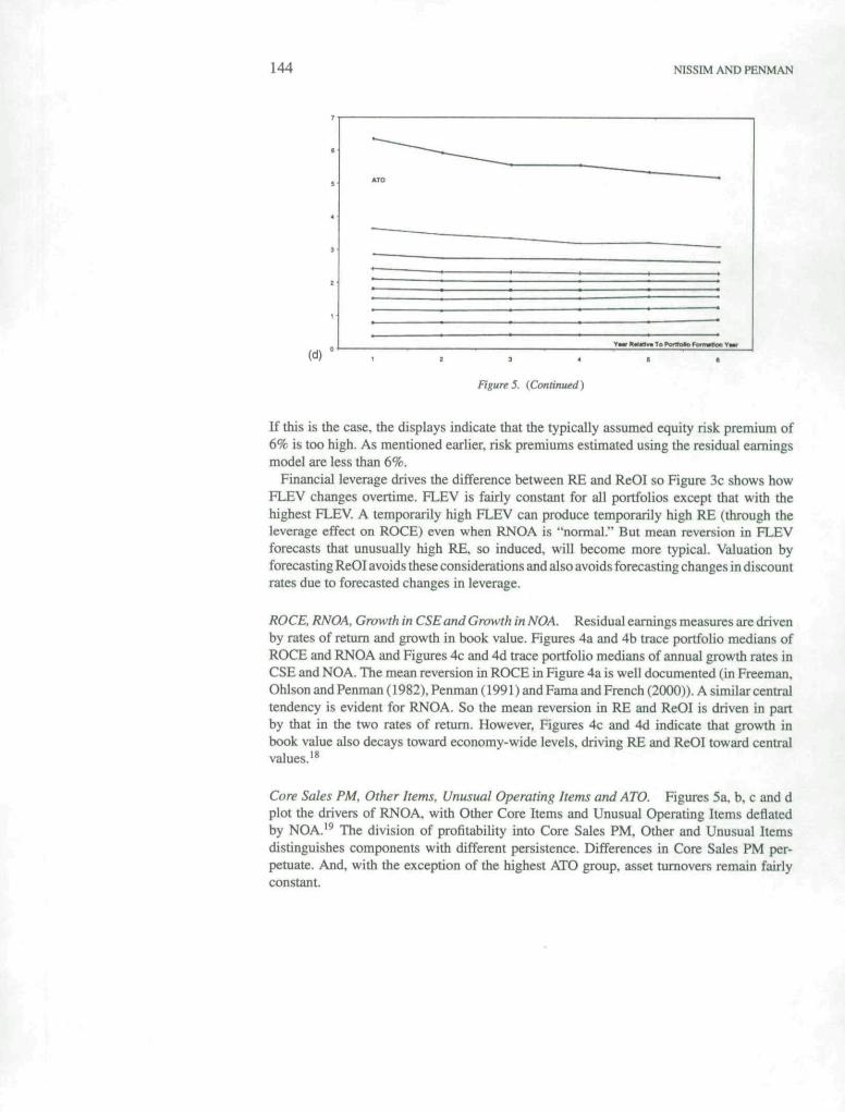
We examine these issues by reference to the displays in Figures 3,4,5 and 6, along withsimple rank correlation measures. The displays are based on ranking a given measure in abase year, year 0, forming 10 portfolios from the rankings, and then tracking median valuesfor each portfolio for the following five years. The ranking is done seven times, in 1964,1969, 1974, 1979, 1984, 1989 and 1994. For each of these years, portfolio medians arecalculated for the ranking year and for the following five years. At end of the five yearsthe ranking is done again for the next five years, and so on until 1994. The figures give themean of portfolio medians over ihe seven sets of calculations. The patterns depicted are quiterobust over the seven time periods, however. The displays are offered with one caveat. Firmsin the base year that do not survive are not in the calculations in yean; after they drop out.Thus the expost averages may be biased estimates of exante amounts for going concerns.

The displays are to be read in conjunction with Table 3.That table gives the Spearman rankcorrelations between ratios and their /-lagged values (r = 1,2,. . . , 5), calculated using allfirm-year observations (1963-1999). It also gives the ratio of the variance of the portfoliomeasures in year tit = 1. 2 , . . . , 5) with that in the base year (year 0), as an indication (atthe portfolio level) ofthe speed of conversion toward a common amount. The correlationsare analogous to R~ in a linear regression and the variance ratios are analogous to a slopecoefficient.


(a)

(C) .,

Figure 3. (a) Evolution of RE over time, (b) Evolution of ReOI over time. <e) Evolution of FLEV over time.


(b) ^,

Figure 4. (a) Evolutior of ROCE over time, (b) Evolution of RNOA over tiine. (c) Evolubon of growth in CSEover time, (d) Evolution of growth in NOA over time.


Figure4. {Continued)

Residual Earnings (RE), Residual Operating Income (ReOI) and FLEV. Figures 3a and3b give the average behavior of median RE and ReOI over five years from the base year.Both are per dollar of average book value (CSE and NOA respectively) in the base year.Both are calculated with a cost of capital equal to the one-year risk-free rate at the beginningof the year plus 6%, but the patterns are similar wben the cost of capital for tbe subsequentyears is the risk-free rate for the future year that is implied in the term structure at the endof the base year, plus 6%.

The following observations are made for both RE and ReOI. First current residua! earningsforecast future residual earnings, not only in the immediate future but five years ahead. Highresidual earnings firms (in tbe cross section) tend to have high residual earnings iater and lowresidual earnings firms tend to have low residual earnings later. Indeed, the rank correlationsin Table 3 between RE in year 0 and RE in years 1,2,3,4 and 5 for individual firms are 0,55,0.37, 0.25, 0.20, and 0.18, respectively. The corresponding rank correlations for ReOI are0.65, 0.50, 0,40. 0,35, and 0.33. Second, in both the figures, tbe decaying rank correlations,and the decaying variance ratios indicate residual earnings tend to converge to central values,with the more extreme becoming more typical over time. But third, permanent levels arenot zero for a number of portfolios. It appears that continuing values of the type CV2 andCV02 (or CV3 and CV03) are typical, not CVl or CVOl. A nonzero permanent level ofresidual earnings can be explained by persistent nonzero net present value investing or byconservative or liberal accounting. Fourth, long-run growth in residual earnings is slightlypositive, suggesting that continuing value calculations of the type CV3 and CV03 mayimprove upon CV2 and CV02.

One other aspect of Figures 3a and 3b warrants mention. The majority of firms havenegative RE or ReOI by the fifth year. Re and ReOI are determined in part by the cost ofcapital. With conservative accounting practiced on average, one expects long-run RE andReOI to be, on average, positive and ROCE and RNOA to be greater than the cost of capital.


(a)

tmr ntmat* To NHVOHO PonnMtor Tav

(b) , „

(C)

Figure 5. (a) Evolution of core sales PM over time, (b) Evolution of other core items/NOA over time,(c) Evolution of UOI/NOA over time, (d) Evolution of ATO over time.


(d)VHt Raunn Te PwVDta FormMMn Vaar

Figure 5. {Continued)

If this is the case, the displays indicate that the typically assumed equity risk premium of6% is too high. As mentioned earlier, risk premiums estimated using the residual eamingsmodel are less than 6%.

Financial leverage drives the difference between RE and ReOI so Figure 3c shows howFLEV changes overtime. n..EV is fairly constant for all portfolios except that with thehighest PT..EV. A temporarily high FLEV can produce temporarily high RE (through theleverage effect on ROCE) even when RNOA is "normal." But mean reversion in FLEVforecasts that unusually high RE, so induced, will become more typical. Valuation byforecasting ReOI avoids these considerations and also avoids forecasting changes in discountrates due to forecasted changes in leverage.

ROCE, RNOA, Growth in CSE and Growth in NOA. Residual earnings measures are drivenby rates of retum and growth in book value. Figures 4a and 4b trace portfolio medians ofROCE and RNOA and Figures 4c and 4d trace portfolio medians of annual growth rates inCSE and NOA. The mean reversion in ROCE in Figure 4a is well documented (in Freeman,Ohison and Penman (1982), Penman (1991) and Fama and French (2000)). A similar centraltendency is evident for RNOA. So the mean reversion in RE and ReOI is driven in partby that in the two rates of retum. However, Figures 4c and 4d indicate thai growth inbook value also decays toward economy-wide levels, driving RE and ReOI toward centralvalues.'^

Core Sales PM, Other Items, Unusual Operating Items and ATO. Figures 5a, b, c and dplot the drivers of RNOA, with Other Core Items and Unusual Operating Items deflatedby NOA.'^ The division of profitability into Core Sales PM. Other and Unusual Itemsdistinguishes components with different persistence. Differences in Core Sales PM per-petuate. And, with the exception of the highest ATO group, asset turnovers remain fairlyconstant


(c)

Figure 6. (a) Evolution of sales growth rate PM over time, (b) Evolution of change in core sales profil marginover time, (c) Evolution of change in ATO over time.


As indicated in Section 2.4, forecasting that profit margins and ATO will be constantssimplifies the forecast of growth: the growth rate in ReOI for a continuing value calculationis then detennined solely by forecasting growth in sales.

Changes in Sales, Core Sales PM and ATO. The Figure 5 graphs are for portfolios formedfrom the cross section. Figure 2c indicates systematic differences in profit margins andturnovers across industries, so ihe differences in the long-run profit margins and ATOs inFig:ure 5 are probably due to permanent differences in technology and cost structure across

Table 3. Summary measures for the evolurion of ratios.

Year; Relative to Base Year

RE

ReOI

FLEV

ROCE

RNOA

Growth in CSE

Growth in NOA

Core Sales PM

Other Core Items/NOA

Unusual Items/NOA

ATO

Growth in Sales

ACore Sales PM

AATO

con,var,/varo

corr,var,/varn

corr,var,/varo

COIT,

var,/varo

corr,var,/varo

COTTf

var, /varo

corr,varr/varo

corr,var,/varo

con,var,/varo

con.var,/varo

con.var,/varo

corr,var,/varo

corr.var, /varo

corr.var,/varo

i

0.5510.441

0.6530.705

0.9370.900

0.6180.372

0.6650.534

0.6590.408

0.5840.318

0.8280.808

0.6630.645

0.3760.128

0.9470.850

0.3090.073

-0.0390.013

0.1660.031

"1

0.3720.241

0.4960.549

0.8460.772

0.4250.183

0.4850.318

0.3070.088

0.1650.025

0.7250.691

0.5330.422

0.2840.058

0.8940.739

0.1150.012

-0.0830.010

-0.1000.024

3

0.2570.165

0.3970.501

0.7810.674

0.3110.100

0.3770.204

0.1900.038

0.0740.011

0.6640.617

0.4510.311

0.2230.031

0.8570.720

0.1030.011

-0.0590.003

-0.0820.010

4

0.2000.188

0.3490.473

0.7350.583

0.2530.080

0.3200.155

0.1290.024

0.05!0.008

0.6280.555

0.4060.243

0.2120.037

0.8300.662

0.1060.008

-0.0430.001

-0.0390.003

5

0.1760.209

0.3270.568

0.7000.526

0.2300.067

0.2980.127

0.1050.020

0.0510.006

0.6050.534

0.3670.195

0.1890.020

0.8080.602

0.1150.007

-0.0120.001

-0.0090.003

Corr, is the Spearman rank corretalion between each ratio and its r-lagged value calculated using all firm-yearobservations(l963-I999). The variance ratio is based on the portfolio analysis. Thi.i analysis is done by formingten ponfolios from a ranking on a ratio in a base year, and calculating the median ratio for each ponfolio in ihebase year and eacb of the subsequent five years. (The base years are 1964. 1969. 1974, 1979, 1984. 1989 and1994.) Next, mean.s of portfolios' medians over the seven replications are calculated (Figures .3a-6c plot thesemeans), var, is the variance of the mean of portfolios' medians in year r. Thus, var,/varo measures the speed ofmean reversion.


industries. So Figures 6a, b and c picture the evolution of changes in sales. Core Sales PMand ATO.

The pattems indicate that unusual charges are indeed transitory. Figure 6b also indicatesthat Core Sales PM can contain further transitory income (after isolating unusual items)and this is detected by looking at changes.^" Similarly, changes in ATO are mean reverting,and rapidly so."'

Table 3 and the supporting displays incorporate all firms that survive to each forwardyear. If the survival rate differs over the portfolios or the reason for non-survival differs,these expost representations may be biased depictions of exante pattems. Correcting for anyeffect of attrition is problematical. One might include expost liquidating eamings for firmsthat drop out but exante forecasts are usually made for going concems (without anticipationof the effects of termination).

Panel A of Table 4 gives the average survival rates for the 10 residual eamings portfoliosin Figure 3a. The numbers in the table are averages over the seven replications (1964-1969,

Table 4. Percentage survivorship rates for residua] eamings poitfolios.

Year t Relative to Base Year: I

Panel A: Percentage survivorship rates

Portfolio:10 (high RE) 97.849 97.571 97.387 96.756 97.335 97.464 97.673 96.772 95.80l(lowRE) 94.13

Portfolio:10 (high RE) 78.009 93.338 100.007 96.676 100.005 90.004 90.003 95.002 77.50I (low RE) 66.57

Panel A repons average (over the seven replications: 1964-1969 1994-1999) of the per-cenlage of finns in each of the 10 residual eamings (RE) portfolios that survived in the respectiveyear after the base year.

The main four reasons for non-surviving are mergers, exchange of stock, liquidation and delist-ing. Panel 8 gives the percentage of non-surviving firms due to a merger or exchange out of ailnon-surviving firms for which the reason of non-survival is reponed in CRSP.

94.6695.4995.5294.7794.9894.7895.7994 J 691.9789.90

QFff uUff t\

87.3395.2696.00%.4797.9092.4695.0093.7590.5771.23

91.7493.5993.3292.2991.9592.5093.3491.1388.2784.83

0 tficf^€r or £

88.71%.5596.5895.8298.0293.8196.5694.8993.1474.20

89.3091.0190.7789.7389.8389.2589.7987.3984.7480.58

xchange

89.93%.5597.4595.8497.3895.9896.0695.4192.7775.78

85.4587.4187.6186.4785.7685.5785.4782.1779.6375.94

88.7396.0597.5695.9997.4496.3796.7995.3289.4472.73


1969-1974 1994-1999) of the percentage of firms iti each of the 10 portfolios in thebase year that survived in each of the subsequent 5 years. Stirvivorship rates are similaracross all portfolios except the bottom two (with the lowest RE). Patterns for all groupsare conditional upon survival, but. for these two groups, the forecaster must be particularlyconcerned with forecasting survivorship as well as forecasting drivers. The main reasons fornon-surviving are mergers, exchange of stock, liquidation and delisting. Panel B of Table 4gives the percentage of tenninations due to merger or exchange, as indicated by CRSP.Myers (1999) indicates that mergers and exchanges result in considerably higher payoffsthan liquidation or delisting and, indeed, higher payoffs than those of surviving firms. Thelower residual eamings portfolios have fewer mergers and exchanges (and more delistingsand liquidations). And the "fade diagrams," like Figure 3a. do not capture the higher payoffsto mergers and exchanges.

4. Conclusion

This paper has laid out a structured financial statement analysis that facilitates forecastingand valuation. The analysis involves an analysis of profitability and an analysis of growth.The analysis of profitability extends the traditional analysis, the analysis of growth comple-ments it: profitability and growth drive equity values. The analysis is guided by the residualeamings valuation model but is appropriate for forecasting free cash flows and dividends ifother valuation approaches are adopted.

Section 2.7 summarizes the major features of the scheme. The overall perspective is oneof forecasting (and, from forecasts, valuation) so financial statement analysis is depicted, asa matter of first order, as an analysis of the future. Ratios are identified as drivers of futureresidual eamings., free cash flow and dividends. Ratios in current financiai statements arethen viewed as information to forecast the future drivers.

The paper documents typical values for ratios and typical pattems for ratios over time.The broad general descriptions are benchmarks that establish priors for forecasting. Theyare input to a more contextual analysis (of industries and firms) and a more sophisticatedeconometric forecasting analysis. The overall feature of the accounting data is centraltendency—convergence of drivers to a common level in the cross section—which bodeswell for calculating continuing values with standard valuation techniques.

The analysis docs not deal with uncertainty in forecasting. This is incorporated in valuationmodels through the discount rate (or discounts from expected values) and one conjecturesthat financial statement analysis is also relevant for determining the discount rate.

Accounting research is concemed with assessing the "information content" of finan-cial statements, presumably with a view to developing concrete products that can beused in practice. The practical significance of this paper should be obvious. But the anal-ysis also guides future research. For forecasting research that applies the predictiveability criterion to evaluate information content the analysis indicates what is to be fore-casted if the researcher has valuation in mind. It also identifies the accounting informa-tion that drives the forecast and the form it might take. The empirical analysis here isvery much at the descriptive level but, with thought, may lead to more formal, parsimo-nious forecast modeling which brings more sophisticated econometrics to the task. Sim-ilarly, the analysis aids in the development of accounting-based valuation models that


go beyond eamings and book values. And it guides the specification of "capital mar-kets regressions" that conduct empirical tests of information contem and accounting-basedvaluation.

Appendix: Notation and Variables Measurement

This appendix describes how the variables are measured. Since perfect identification ofoperating and financing items requires data that are not available on Compustat, some ofthe variables are measured with error. When applicable, we discuss measurement issuesbelow the variable's definition.

Financial Assets (FA) = cash and short term investments (Compustat #1)

plus investments and advances-other (Compustat #32).

Companies hold cash on a regular basis partially because they cannot perfectly synchro-nize cash receipts and disbursements. Thus, a portion of "cash and short-term investments"is an operating asset. But we cannot separate the operating portion of cash from the total ofcash and short-term investments, and we cannot separate interest income on operating cashfrom total interest income. So we classify all cash as a financial asset.

There are generally two types of investment securities: debt and equity. Investments in debtsecurities are financial assets, but investments in equity securities are usually investments inthe operations of affiliated companies, and thus are operating assets. Compustat reports long-term investments in debt securities together with long-term investments in equity securities(other than those accounted for by using the equity method). Since most investments (otherthan those accounted for using the equity method) are in debt securities, we classify theitem "investments and advances—other" (#32) as part of financial assets.

Another measurement issue is that "investments and advances—other" (#32) includeslong-term receivables that are related to operating activities. However, receivables are usu-ally carried close to their value even when they relate to operating activities (e.g., long-termlease receivables). More importantly, interest income on alt receivables is included in interestincome, which is classified as financial income (see below).

Operating Assets (OA) = Total Assets (TA, Compustat #6) minus Financial Assets (FA).

Financial Obligations (FO) = debt in current liabilities (#34) plus long term debt (#9)plus preferred stock (#130) minus preferred treasury stock (#227) and plus preferreddividends in arrears (#242).

Net Financial Obligations (NFO) = Financial Obligations (FO) minus Financial Assets(FA).

Common Equity (CSE) = common equity (#60) plus preferred treasury stock (#227) minuspreferred dividends in arrears

Net Operating Assets (NOA) = Net Financial Obligations (NFO) plus Common Equity(CSE) and plus Minority Interest (MI, #38)


Operating Liabilities (OL) = Operating Assets (OA) minus Net Operating Assets (NOA).

Core Net Financial Expense (Core NFE) = after tax interest expense (#15 x (1 — marginaltax rate)) plus preferred dividends (#19) and minus after tax interest income (#62 x(1 — marginal tax rate)). '

Unusual Financial Expense (UFE) = lag marketable securities adjustment (lag #238) minusmarketable securities adjustment (#238).

Due to data problems we cannot include gain/loss on early extinguishment of debt, acomponent of UFE, in our measure of UFE. This item is classified as an extraordinaryitem and Compustat provides only the total of extraordinary items with no information ontheir nature. So we include all extraordinary items in operating income. In any case, ourclassification excludes extraordinary items from core income.

Another data issue with the measurement of UFE is that cumulative translation adjustment,a dirty stupius equity account, reflects unrealized currency translation gains and losses notonly on operating items, but also on financial assets and liabilities. COMPUSTAT (and oftenthe financial reports) does not provide enough details to separate the two. Since NOA areusually larger than NFO, we include this income item in operating income (see below).

Net Financial Expense (NFE) = Core Net Financial Expense (Core NFE) plus UnusualFinancial Expense (UFE).

Clean Surplus Adjustments to net income (CSA) = marketable securities adjustment (#238)minus lag marketable securities adjustment (lag #238) plus cumulative translation ad-justment (#230) and minus lag cumulative translation adjustment (lag #230).

CSA should include all items that change common equity and bypass the income statement(dirty surplus items) other than net dividends. Compustat provides information on thecumulative balance of two dirty stirplus items: translation gains and losses (;G30) andunrealized gains and losses on financial items (#238). Thus, CSA may be estimated as thechange in these items during the year. These two items, although the more common andmaterial dirty surplus items, are not the only ones.

An altemative approach to calculating CSA is by analyzing the change in retained eam-ings. That is. CSA equals the change in retained eamings minus net income and plus netdividends. There are several problems with this approach, however. The main problem isthat stock dividends, share retirements and share repurchases (when accounted for usingthe par value method) reduce retained eamings but are not

Comprehensive Net Income (CNI) = net income (#172) minus preferred dividends (#19)and plus Clean Surplus Adjustment to net Income (CSA).

Comprehensive Operating Income (01) = Comprehensive Net Financial Expense (NFE)plus Comprehensive Net Income (CNT) and plus Minority Interest in Income (Mil,

Some parts of dirty surplus income (e.g.. currency translation gains and losses) are associ-ated with minority interests, but COMPUSTAT (and often financial reports) do not provide

RATIO ANALYSIS AND EQUTTY VALUATION 1 5 1

the detaiis necessary to adjust minority interest income for dirty surplus items. So minorityinterest income, and therefore operating income, are misstated. However, since minorityinterest is usually very small, the effect of this misstatement is likely to be immaterial formost companies.

Unusual Operating Income (UOI) = after tax nonoperating income (expense) excludinginterest and equity in earnings ((#190 — #55) x (1 — marginal tax rate)) plus aftertax special items (#17 x (1 — marginal tax rate)) plus extraordinary items & discon-tinued operations (#48) plus cumulative translation adjustment (#230) and minus lagcumulative translation adjustment Oag #230).

Other Operating Income Items (Other Items) = Equity in earnings (#55).

Operating Income from Sales (OI from Sales) = Operating Income (01) minus OtherOperating Income Items (Other Items).

Core Operating Income from Sales (Core 01 from Sales) = Operating Income from Sales(01 from Sales) minus Unusual Operating Income (UOI).

Marginal Tax Rate = the top statutory federal tax rate plus 2% average state tax rate. The topfederal statutory corporate tax rate was 52% in 1963. 50% in 1964,48% in 1965-1967,52.8% in 1968-1969. 49.2% in 1970. 48% in 1971-1978, 46% in 1979-1986,40% in1987, 34% in 1988-1992 and 35% in 1993-1999.

Interest on Operating Obligations (io) = the one year risk-free rate at the beginning ofthe year multiplied by the difference between operating liabilities (OL) and "DeferredTaxes and Investment Tax Credit" (#35).

A more precise calculation of io would not impute implicit interest on the accrued pensioncost but instead add the net interest cost on the net pension obligation (i.e., interest costminus actual return on plan assets). However. Compustat gives details about the pensioninterest cost and the actual return on plan assets only starting 1991, and it does not providethe net accrued pension cost. This liability is probably included in item #75 (liabilities—other).

Acknowledgments

The comments of Trevor Harris, Charles Lee, Jim Ohlson (and his teaching notes), KatherineSchipper and Toshi Shibano were helpful.

Notes

1. Variaiion in outcomes for different scenarios also indicate.<i risk.2. For Hnancial inslitutions. "financial" asseu and liabilities are operating assets and liabilities. Financial insti-

tutions are excluded from our empirical analysis.3. Johannson (1998) distinguishes operating and linancing liabilities and the role they play in profitability analysis,

but does not develop the formal analysis of operating liability leverage here.


4. Deferred taxes are not discounted (and the govemment does not implicitly charge interest). Net interest costof pension liabilities is explicit in the income statement So, with these items on the balance sheet,

io = shon-terrn borrowing rate x OL other than deferred taxes and pensions

+ net interest cost on pension liabiliues.

5. When there are minority interests, an additional driver is the ratio of minority interests to common equity.6- For V^"^ and V^'^ to be added as separate values and be equivalent to (1), it is required that

yN!=O

PE=PW + -~^ X [pw - PD]

(which is the same form as (4)). That is, the cost of capital for operations is

as in standard finance that evokes Modigliani and Miller financing irrelevance (without consideration of taxeffects from the financing). The distinction between different costs of capitai for dilTereni net assets is somewhatcosmetic for the purposes of this paper, as the ratio analysis and the d(Kumentation that follows do not concernthe cost of capita!. The observation that different income streams have different risks (and thus different COSLSof capitai) is standard in finance texts and we adhere to this orthodoxy largely so as to not offend the eye.

7. Growth in residual eamings translates into a P/E ratio, the multiple commonly used to indicate growth.Forecasting constant RE yields a normal /*/£ ratio (equal to/?£/(/)£• — 1)) and forecasting growing RE yieldsa P/f ratio greater than normal. See Penman (1996).

8. Free cash flow treats growth in NOA (ANOA) as a negative driver (it is subtracted in (14)) whereas residualincome treats investment as a positive driver. This identification is the main difference between residual incomeand discounted cash flow techniques.

9. Again, if minority interests exits, equation (16) is a decomposition of ROTCE, not ROCE.10. The analysis omits effects on .shareholder value of taxes on dividends and the value effects of the tax-

deductibility of interest on dcbi. if any. GAAP oniiLs the calculation of the cost to shareholders of employeestock options but this is a matter of recognizing an expense in comprehensive income. I[ does not affect ihedecomposition.

11. Except for the calculation of NBC and Core NBC, since firms can have negative net financial obligation.s (thatis, net financial asset positions).

12. Some firms adopted the Statement in 1993.13. The median growth rates for RE and ReOI in Table 1 are negative. Growth rates are calculated only for the

cases of positive denominators, li will become clear in the time-series analysis that follows that these residualincome measures subsequently decline, on average, for firms with positive residual income.

14. The product-moment (Pearson) correlation between median ROCE and the treasurj- yield is 0.32. The correla-lion between the lagged median ROCE and the treasury yield i.s 0.67. The one-year treasury yield is measuredat the beginning of the year. Thus ROCE is more strongly related to the yield at Ihe end of the year than to theyield at the beginning of the year.

15. In constructing these figures, a few extreme observations were deleted.16. Ohlson and Zhang (1999) and Pentnan (1997) model finite-horizon residual eamings valuation.17. See, for example. Frankel and Lee (1998), Lee. Myers and Swaminathan (1999), Penman and Sougiannis

(1998), and Francis, Olsson and Oswald (2000).18. Survivorship bias is a particular concern in interpreting Figures 4c and 4d. however. CSE and NOA increase

through acquisitions and such growth is incorporated in the nutnbers here. But the negative growth of firmsacquired is not,

19. Figure 5b includes only non-zero Other Core Items.20. The pattern for the largest negative change in Core Sales PM in yearO is particularly interesting. This portfolio

has the largest (positive) changes in subsequent years. Is this "big bath" accounting that shifts income to thefuture?


2L The persistence of ATO changes for one period here \s partly due to using average NOA in the calculation ofATO.

22. The eff'ect of stock dividends on retained earnings is included in item #231 (Retained Earnings—OtherAdjustments). This item also includes the effect of notes receivable (presumably for share issues). Bothitems are not income items, and thus the change in #231 should be the deducted from the change in retainedearnings. The problem is that this item is available only starting 1982.

References

Abarbanell. J. S.. and V. L. Bernard. (2000). "Is the U.S. Stock Mariiet MyopicT' Joumal of Accounting Research38.221-243.

Beaver. W. H., and S. G. Ryan. (2000). "Biases and Lags in Book Value and their Effects on the Abil-ity of ihe Book-to-Market Ratio to Predict Book Retum on Equiiy." Joumal of Accounting Research 38,127-148.

Brief. R. P.. and R. A. Lawson. (1992). "The Role of the Accounting Rate of Retum in Financial StatementAnalysis." Tiie Accounting Review 67. 411-426.

Brown. L. D. (1993). "Earnings Forecasting Research: Its Implications for Capital Markets Research."/ntrman'ono/Journal of Forecasting 9, 295-320.

Brown. S. J.. W. N. Goetzmann. and S. A. Ross. (1995). "Survival." Journal of Finance 50. 8.53-873.Claus. J. } . , and J. K. Thomas. (2(X)I). "Equity Premium as Low as Three Percent? Evidence from Analysists*

Earnings ForecasLs for Domestic and [ntemational Stocks" Joumal of Finance. Forthcoming.Colander. D. (1992). "Retrospectives: The Lost Art of ônamicf,!' Journal of Economic Perspectives 6. 191-198.Edwards. E. 0.. and P. W. Bell, (1961). The Theory and Measurement of Business Income. Berkeley, CA: The

University of California Press.Fairfield. P. M.. R. J. Sweeney, and T. L. Yohn. (1996). "Accounting Classification and the Predictive Content of

Earnings." Vie Accounting Review 11, 337-355.Fama E. F.. and K. R. French. (2000). "Forecasting Profitability and Earnings." Joumal of Business 73.Feltham. G. A., and J. A. Ohlson. (1995). "Valuation and Clean Surplus Accounting for Operating and Financial

Activities." Contemporary Accounting Research 11. 689-731.Francis. J.. P. Olsson. and D. R. Oswald. (2000). "Comparing the Accuracy and Explainability of Dividend, Free

Cash Flow, and Abnormal Earnings Equity Value Estimates." Journal of Accounting Research 38. 45-70.Frankel, R., and C. M. C. Lee. (1998). "Accounting Valuation, Market Expectation and Cross-Sectional Stock

Keiums." Jour/uil of Accounting and Economics 25. 283-319.Freeman. R. N.. J. A. Ohlson. and S. H. Penman. (1982). "Book Rate-of-Retum and Prediction of Earnings

Changes: An Empirical Investigation." Joumal of Accounting Research 20. 639-653.Gebhardt. W. R.. C. M. C. lê. and B. Swaminalhan. (2000). 'Toward an implied Cost of Capital." youma/o/

Accounting Research, Forthcoming.Graham. B.. D. L. Dodd. and S. Cottle. (1962). Security Analysis. New York, NY: McGraw-Hill Book Company,

Inc.Ibbouson. R.. and R. Sinquefield. (1983). Stocks, bonds, bills and injiation. 1926-1982. Charlotiesville. VA:

Financial Analyst Rej;earch Foundation.Johansson. S. (1998). The Profitability. Financing, and Growth ofthe Firm: Goals, Relationships and Measurement

Methods. Lund. Sweden: Studentlilteratur.Kay, J. A. (1976). "AccountanLs. too. Could be Happy in a Golden Age: Tlie Accountants Rate of Protit and the

Internal Rate of Retum." Oxford Economic Papers 17.447-460.Lee C. M. C , J. Myers, and B. Swaminathan. (1999). "What Is [he Intrinsic Value of the Dow?" Joumal of Finance

54, 169.3-1741.Lew B.. andS. R. Thiagarajan. (1993). "Fundamental Information Analysis." yoMma/o/;4croa«rin^êjforc/i 31,

190-215.Lipe, R. C. (1986). "The Information Contained in the Components of Earnings." Journal of Accounting Research

24,37-64.Myers. J. N. (1999). "Conservative Accounting and Finite Ftrm Life: Why Residual Income Valuation Estimates

Understate Stock Price." Working Paper. University of Washington.Ohlson. J. A. (1995). "Earnings, Book Values, and Wvidends in Equity Valuation." Contemporary Accounting

Research 11,661-687.

154 NiSSIM AND PENMAN

Ohlson J. A., and X. J. Zhang. (1999). "On the Theory of the Forecast-Horizon in Equity Valuation."Accounling Research 37.437—449.

O'Hanlun J.. and A. Steele. (1998). "Estimating the Equity Risk Premium Using Accounting Fundamenmis."Working Paper, Lancaster University.

Ou. J. A. (1990). "The Information Content of Noneamings Accounting Numbers as Eamings Predictors." Journalof Accounting Research 28, 144-163.

Ou. j . A., andS. H. Penman. (1989). "Financial Statement Analysis and the Prediction of Stock Returns'' Journalof Accounting and Economics 11, 295-329.

Ou, J. A., and S. H. Penman. (1995). "Financial Statement Analysis and the Evaluation of Markct-to-Book Ratios."Woiidng Paper. Universiiy of Califumia at Berkeley.

Penman. S. H. (1996). "The Aniculation of Price-Eamings Ratios and Market-to-Book Ratios and the Evaluationof Growih." Journal of Accounting Research 34, 235-259.

Penman. S. H. (1991). "An Evaluation of Accounting Rate-of-Reium." Journal of Accounting, Auditing, andFinance 6. 233-255.

Penman S. H. (1997). "A Synthesis of Equity Valuation Techniques and the Terminal Value Calculation of theDividend Discount Model." Review of Accounting Studies 2, 303-323.

Penman S. H., and T. Sougiannis. (1998). "A Comparison of Dividend, Cash Row, and Eamings Approaches toEquity Valuation." Contemporary Accounting Research 15, 343-383.

Preinreich, G. (1938). "Annual Survey of Economic Theory: The Theory of Depreciation." Econometrica, 219-241.

Selling, T.I..and C P. Stickney. (1989). "The Effects of Business Environments and Strategy on a Firm's Rate ofRetum on Assets." Financial Analysts Joumal, 43-52.

Zhang, X. (20(X)). "Conservative Accounting and Eamings Valuation." Joumal of Accounting andEconomics 29, 125-149.

Date post:	03-Dec-2015
Category:	Documents
Upload:	firebirdshockwave
View:	24 times
Download:	1 times

Ratio Analysis and Equity Valuation From Research to Practice.

Documents