Rational IPO Waves · LUBO · SP ¶ ASTOR and PIETRO VERONESI * ABSTRACT We argue that the number of ¯rms going public changes over time in response to time variation in market conditions. We develop a model of optimal IPO timing in which IPO waves are caused by declines in expected market return, increases in expected aggregate pro¯tability, or increases in prior uncertainty about the average future pro¯tability of IPOs. We test and ¯nd support for the model's empirical predictions. For example, we ¯nd that IPO waves tend to be preceded by high market returns and followed by low market returns. * Both authors are at the Graduate School of Business, University of Chicago. Both are also a±liated with the CEPR and NBER. Helpful comments were gratefully received from Malcolm Baker, John Campbell, John Cochrane, George Constantinides, Doug Diamond, Frank Diebold, Gene Fama, John Heaton, Jean Helwege, Steve Kaplan, Jason Karceski, Martin Lettau, Deborah Lucas, Robert Novy-Marx, Michal Pako· s, Jay Ritter, Tano Santos, Rob Stambaugh, Per StrÄ omberg, Ren¶ e Stulz, Lucian Taylor, Dick Thaler, Luigi Zingales; an anonymous referee; seminar participants at Bocconi University, Comenius University, Duke University, Federal Reserve Bank of Chicago, HEC Montreal, INSEAD, London Business School, MIT Sloan, Rice University, University of Brescia, University of Chicago, University of Illinois at Urbana-Champaign, University of Pennsylvania, University of Southern California, Vanderbilt University; and the conference participants at the Fall 2003 NBER Asset Pricing Meeting and the 2004 Western Finance Association Meetings. Huafeng Chen, Karl Diether, Lukasz Pomorski, and Anand Surelia provided expert research assistance. This paper previously circulated under the title \Stock Prices and IPO Waves."
Transcript
Rational IPO Waves
·LUBO·S P¶ASTOR and PIETRO VERONESI*
ABSTRACT
We argue that the number of ¯rms going public changes over time in response to time
variation in market conditions. We develop a model of optimal IPO timing in which IPO
waves are caused by declines in expected market return, increases in expected aggregate
pro¯tability, or increases in prior uncertainty about the average future pro¯tability of IPOs.
We test and ¯nd support for the model's empirical predictions. For example, we ¯nd that
IPO waves tend to be preceded by high market returns and followed by low market returns.
*Both authors are at the Graduate School of Business, University of Chicago. Both are also a±liated
with the CEPR and NBER. Helpful comments were gratefully received from Malcolm Baker, John Campbell,
John Cochrane, George Constantinides, Doug Diamond, Frank Diebold, Gene Fama, John Heaton, Jean
Helwege, Steve Kaplan, Jason Karceski, Martin Lettau, Deborah Lucas, Robert Novy-Marx, Michal Pako·s,
Jay Ritter, Tano Santos, Rob Stambaugh, Per StrÄomberg, Ren¶e Stulz, Lucian Taylor, Dick Thaler, Luigi
Zingales; an anonymous referee; seminar participants at Bocconi University, Comenius University, Duke
University, Federal Reserve Bank of Chicago, HEC Montreal, INSEAD, London Business School, MIT Sloan,
Rice University, University of Brescia, University of Chicago, University of Illinois at Urbana-Champaign,
University of Pennsylvania, University of Southern California, Vanderbilt University; and the conference
participants at the Fall 2003 NBER Asset Pricing Meeting and the 2004 Western Finance Association
Meetings. Huafeng Chen, Karl Diether, Lukasz Pomorski, and Anand Surelia provided expert research
assistance. This paper previously circulated under the title \Stock Prices and IPO Waves."
The number of initial public o®erings (IPOs) changes dramatically over time, as shown in
Figure 1. For example, 845 ¯rms went public in the United States in 1996, but there were
only 87 IPOs in 2002. Although the °uctuation in IPO volume is well known (e.g., Ibbotson
and Ja®e (1975)), its underlying causes are not well understood. Many researchers attribute
time variation in IPO volume to market ine±ciency, arguing that IPO volume is high when
shares are \overvalued."1 Such an argument assumes that the periodic market mispricing
can somehow be detected by the owners of the ¯rms going public, but not by the investors
providing IPO funds. In contrast, we present a model in which °uctuation in IPO volume
arises in the absence of any mispricing, and in which IPO volume is more closely related to
recent changes in stock prices than to the level of stock prices.
******************** INSERT FIGURE 1 HERE ********************
We develop a model of optimal IPO timing in which IPO volume °uctuates due to time
variation in market conditions. We de¯ne market conditions as having three dimensions: ex-
pected market return; expected aggregate pro¯tability; and prior uncertainty about the post-
IPO average pro¯tability in excess of market pro¯tability, henceforth referred to as \prior
uncertainty." Market conditions indeed appear to vary in these dimensions. Time variation
in expected market return is consistent with empirical evidence on return predictability.2
Time variation in expected aggregate pro¯tability is related to business cycles. Time varia-
tion in prior uncertainty seems plausible as well. For example, technological revolutions are
likely to be accompanied by high prior uncertainty, because they make the prospects of new
¯rms highly uncertain. We show, theoretically and empirically, that IPO volume responds to
time variation in all three dimensions of market conditions. Moreover, we note that market
conditions are related not only to IPO volume but also to stock prices, as represented by the
¯rms' ratios of market to book value of equity (M/B). IPO volume is then naturally related
to stock prices as well.
Our model considers a special class of agents, \inventors," who invent new ideas that
can lead to abnormal pro¯ts. Inventors patent each idea and start a private ¯rm that owns
the patent. Inventors possess a real option to take their ¯rms public, invest part of the IPO
proceeds, and begin producing. They choose the best time to exercise this option. When
market conditions are constant, it is optimal to go public as soon as the patent is secured.
When market conditions vary over time, however, inventors may prefer to postpone their
IPO in anticipation of more favorable market conditions.
We solve for the optimal time to go public and show that private ¯rms are attracted to
capital markets especially when market conditions are favorable in the sense that expected
market return is low, expected aggregate pro¯tability is high, and prior uncertainty is high.
1
At any point in time, private ¯rms are waiting for an improvement in market conditions;
that is, for a decline in expected market return or for an increase in expected aggregate prof-
itability or prior uncertainty. When market conditions improve su±ciently, many inventors
exercise their options to go public, thus creating a cluster of IPOs, or an \IPO wave."
To analyze the properties of IPO waves in our model, we calibrate the model to match
some key features of the data on asset prices, pro¯tability, and consumption, and simulate
it over a long period of time. In the simulation, one idea is invented each period, so that
IPO waves do not develop from the clustering of technological inventions in time. Instead,
IPO waves are the result of clustering in the inventors' optimal IPO timing decisions.
Our model makes many empirical predictions. IPO waves caused by a decline in expected
market return should be preceded by high market returns, because prices rise when expected
return falls, and followed by low market returns, because expected return has fallen.3 IPO
waves caused by an increase in expected aggregate pro¯tability should also be preceded by
high market returns, because prices rise as cash °ow expectations go up, and followed by
high pro¯tability, because expected pro¯tability has risen. IPO waves caused by an increase
in prior uncertainty should be preceded by increased disparity between newly listed ¯rms
and seasoned ¯rms in terms of their valuations and return volatilities.
We test the model's implications by using data between 1960 and 2002. Our results
support all three channels (discount rate, cash °ow, and uncertainty) through which IPO
waves are created in our model. We ¯nd that IPO volume is positively related to recent
market returns, which suggests that many ¯rms go public after expected market return
declines or after expected aggregate pro¯tability increases. This result is consistent with both
the discount rate and cash °ow channels. Additional support for the discount rate channel is
provided by the ¯ndings that IPO volume is negatively related to future market returns and
to recent changes in market return volatility. The cash °ow channel is further supported by
the facts that IPO volume is positively related to changes in aggregate pro¯tability and to
revisions in analysts' forecasts of long-term earnings growth. IPO volume is also positively
related to recent changes in two empirical proxies for prior uncertainty.
Another testable implication of our model is that IPO volume is more closely related to
recent changes in stock prices than to the level of stock prices. The relation between IPO
volume and recent changes in prices is due to the endogeneity of IPO timing: Firms are
induced to go public by improvements in market conditions, and these improvements lift
stock prices at the same time. IPO volume is also positively related to the level of stock
prices, as represented by the aggregate M/B ratio, but that relation is weaker. IPO volume
is not necessarily high when the level of stock prices is high because the high price level is
a result of cumulative improvements in market conditions, and many private ¯rms that had
been waiting for such improvements went public while prices were rising. Consistent with
2
these arguments, we ¯nd that IPO volume is signi¯cantly related to recent market returns,
but unrelated to the level of the aggregate M/B ratio.
The evidence of no relation between the level of M/B and IPO volume does not support
the behavioral story in which IPO waves arise when shares are overvalued. This story also
does not predict our ¯ndings that IPO volume is negatively related to changes in market
return volatility, and positively related to changes in aggregate pro¯tability and to changes
in the di®erence between the return volatilities of new and old ¯rms. These ¯ndings do not
disprove the behavioral story, but they suggest that our explanation for IPO waves, which
predicts all of these facts, provides a plausible alternative to the mispricing story.
This paper is related to many earlier studies. Apart from the literature on market
mispricing, cited earlier, this paper is related to the studies that link the volume of equity
issuance to the asymmetry of information resulting from the adverse selection costs of issuing
equity (e.g., Myers and Majluf (1984)).4 Also related is the literature that focuses on the
corporate control aspect of an IPO (e.g., Zingales (1995)).5 This paper abstracts from both
of these important corporate ¯nance issues and shows that IPO volume can °uctuate also
in the absence of asymmetric information and private bene¯ts of control.
This paper is also related to the literature on irreversible investment under uncertainty.6
In our model, the capital raised in the IPO is immediately invested, as it is in the model
of Jovanovic and Rousseau (2001). In their model, the option to delay an IPO is valuable
because waiting allows a private ¯rm to learn about its own production function. In our
model, this option is valuable due to time variation in market conditions. Finally, Boehmer
and Ljungqvist (2004) ¯nd empirical support for our model in German data.
The paper is organized as follows. Section I describes the setting in which IPO decisions
are made. Section II discusses the decision to go public and analyzes some properties of
optimal IPO timing. Section III uses a simulated sample to investigate the properties of
IPO waves in our model. Section IV tests the model's predictions empirically. Section V
examines the relation between IPOs and investment. Section VI concludes.
I. Model
There are two classes of agents, inventors and investors, who have identical information
and preferences but di®erent endowments. Investors are endowed with a stream of consump-
tion good. Inventors are endowed with the ability to invent patentable ideas that can deliver
abnormal pro¯ts. When an inventor patents his idea, he starts a private ¯rm that owns the
patent but produces no revenue. Any time before the patent expires, the inventor can decide
to make the investment that initiates production. To ¯nance this investment, the private
¯rm issues equity to investors in an IPO.
In this section, we describe the economic environment in which IPO decisions take place.
3
This environment features time-varying market conditions, whose three dimensions are de-
scribed in the next three subsections. We then solve for the market value of a ¯rm, which is
an essential input to the optimal IPO timing problem analyzed in Section II.
A. Time-Varying Pro¯tability
After the IPO, ¯rm i's pro¯ts are protected by a patent until time Ti. Let ½it = Y
it =B
it
denote the ¯rm's instantaneous pro¯tability at time t, where Y it is the earnings rate and Bit
is the book value of equity. Motivated by empirical evidence (e.g., Fama and French (2000)),
we assume that ¯rm pro¯tability follows a mean-reverting process between the IPO and Ti:
d½it = Ái¡½it ¡ ½it
¢dt+ ¾i;0dW0;t + ¾i;idWi;t; (1)
where W0;t and Wi;t are uncorrelated Wiener processes that capture systematic (W0;t) and
¯rm-speci¯c (Wi;t) components of the random shocks that drive the ¯rm's pro¯tability. We
also assume that the ¯rm's average pro¯tability ½it can be decomposed as
½it = Ãi+ ½t: (2)
The ¯rm-speci¯c component Ãi, which we refer to as the ¯rm's average excess pro¯tability,
re°ects the ¯rm's ability to capitalize on its patent, and is assumed to be constant over time.
The common component ½t, which we refer to as expected aggregate pro¯tability, is assumed
to exhibit mean-reverting variation:
d½t = kL (½L ¡ ½t) dt+ ¾L;0dW0;t + ¾L;LdWL;t; (3)
where W0;t and WL;t are uncorrelated. Mean reversion in expected aggregate pro¯tability
re°ects business cycles in the aggregate economy.
B. Time-Varying Prior Uncertainty
Average excess pro¯tability Ãiis unobservable. For any ¯rm i that goes public at time t,
all inventors and investors have the same prior belief about Ãi. Their prior uncertainty, b¾t,
is assumed to be the same for all ¯rms going public at time t, for simplicity. It seems plau-
sible for prior uncertainty b¾t to vary over time. For example, uncertainty about the Ãi's ofnew ¯rms is greater when the economy experiences technological advances whose long-term
impact is uncertain. To model time variation in b¾t, we assume that b¾t takes values in the dis-crete set V = fv1; :::; vng and that it switches from one value to another in each in¯nitesimalinterval ¢ according to the transition probabilities ¸hk¢ = Pr
¡b¾t+¢ = vkjb¾t = vh¢.Both inventors and investors begin learning about Ã
ias soon as ¯rm i begins producing
at its IPO. Both learn by observing realized pro¯tability ½it, as well as ½t, ct (de¯ned below),
4
and ½jt for all ¯rms j that are alive at time t. The prior distribution of Ãiis assumed to be
normal, so the posterior of Ãiis also normal, with mean bÃit and variance b¾2i;t. The dynamics
of the posterior moments are given in Lemma 1 in the Appendix. Agents can observe ½t.7
C. Time-Varying Expected Market Return
Let ¹t denote expected market return at time t. To generate time-varying ¹t, we work
with a framework similar to that of Campbell and Cochrane (1999). In this framework, ¹t
varies over time due to the time-varying risk aversion of the representative investor. All
inventors and investors, indexed by k, have habit utility over consumption:
U¡Ckt ; Xt; t
¢= e¡´t
¡Ckt ¡Xt
¢1¡°1¡ ° ; (4)
where Xt is an external habit index, ° regulates the local curvature of the utility function,
and ´ is a time discount parameter.
Let Ct =P
k Ckt denote aggregate consumption, ct = log (Ct), and St = (Ct ¡Xt) =Ct
denote the surplus consumption ratio. Campbell and Cochrane assume that st = log (St)
follows a mean-reverting process with time-varying volatility and perfect correlation with
unexpected consumption growth. This speci¯cation allows Campbell and Cochrane to solve
for market prices numerically. To obtain analytical solutions for prices, we assume that
st ´ s (yt) = a0 + a1yt + a2y2t ; (5)
where yt is a state variable driven by the following mean-reverting process:
dyt = ky (y ¡ yt) dt+ ¾ydW0;t: (6)
Time variation in yt generates time variation in both components of ¹t, the equity premium
and the real risk-free rate. As shown in the Appendix, high yt implies a low equity premium
and a low risk-free rate in the plausible range. We show that time variation in either the
equity premium or the risk-free rate leads to time variation in IPO volume.
We assume that markets are dynamically complete, in that shocks to the aggregate state
variables yt, ½t, and b¾t can be hedged using contingent claims. No contingent claims canhedge ¯rm-speci¯c shocks dWi;t, but those shocks can be hedged using ¯rm equity. Since
markets are complete, inventors and investors can perfectly insure each other's consumption.
Assuming that their initial endowments are equally valuable, inventors and investors choose
identical consumption plans, thus justifying the existence of a representative agent with
preferences given in equation (4). The stochastic discount factor (SDF) ¼t is then unique:
¼t = UC (Ct;Xt; t) = e¡´t (CtSt)
¡° = e¡´t¡°(ct+st): (7)
5
In equilibrium, aggregate consumption is given by the sum of all endowments and net
payouts in the economy. Computing this sum is complicated, because the payouts depend
on the inventors' optimal IPO timing. Instead, for tractability, we assume that ct follows
dct = (b0 + b1½t) dt+ ¾cdW0;t: (8)
As other recent studies, we assume that consumption is ¯nanced mostly by income that is
outside our model, and the resulting process is given in equation (8). Consumption growth
is allowed to depend on ½t because such a link is plausible ex ante, but none of our results
rely on this link. The data-implied value of b1 turns out to be small (b1 = 0:08 in Table I),
and b1 = 0 leads to the same conclusions throughout.
D. The Market Value of a Firm
This subsection discusses a closed-form solution for the market value of a ¯rm in the
environment described above. Our pricing analysis extends the model of P¶astor and Veronesi
(2003a) to allow for time variation in market conditions.
After its IPO, ¯rm i earns abnormal pro¯ts (Ãi) until its patent expires at time Ti. We
assume that any abnormal earnings after Ti are eliminated by competitive market forces, so
that the ¯rm's market value at Ti equals its book value, MiTi= BiTi. The ¯rm is assumed
to pay no dividends, to be ¯nanced only by equity, and to issue no new equity.8 The ¯rm's
market value at any time t after the IPO but before Ti is Mit = Et
£(¼Ti=¼t)B
iTi
¤, with ¼t
given in equation (7). An analytical formula for M it is provided in Proposition 1 in the
Appendix, together with expressions for the ¯rm's expected return and volatility.
The intuition behind the pricing formula is as follows. A ¯rm's M/B is high if
(1) the ¯rm's expected pro¯tability is high
(2) the ¯rm's discount rate is low
(3) uncertainty about the ¯rm's average future pro¯tability is high.
In (1), M/B increases with three cash-°ow related quantities: expected aggregate prof-
itability, ½t; expected excess pro¯tability,bÃit; and current pro¯tability, ½it. In (2), we ¯nd
numerically that M/B increases with the state variable yt in the calibrated model. Since high
yt implies a low risk aversion of the representative investor, it also implies a low expected
market return and high M/B. In (3), M/B increases with b¾i;t, uncertainty about Ãi, as shownby P¶astor and Veronesi (2003a). For more details on the pricing formula, see the Appendix.
Throughout, we say that market conditions improve (worsen) when expected market
(falls). We note that improvements in market conditions raise M/B and vice versa.
6
II. Optimal IPO Timing
This section analyzes the IPO decision. Figure 2 summarizes the sequence of events. At
time ti, a new idea is patented by an inventor.9 Until the patent expires at time Ti, it enables
the owner to earn average excess pro¯tability Ãi. Production requires capital Bti , which is
raised in an IPO. At some time ¿i, ti · ¿i · Ti, the inventor may decide to go public and ¯lethe IPO. The IPO itself takes place at time ¿i+ `, where the lag ` re°ects the time required
by the underwriter to conduct the \road show." In the IPO, the inventor sells the ¯rm
to investors for its fair market value, M i¿i+`, and pays a proportional underwriting fee, f .
Part of the IPO proceeds, Bti, are immediately invested by the inventor and the production
begins, generating the pro¯ts described in equation (1). Once the investment Bti is made,
it is irreversible in that the project cannot be abandoned. The inventor's payo® from going
public is M i¿i+`
(1¡ f)¡Bti, the market value of the patent net of fees.
******************** INSERT FIGURE 2 HERE ********************
The inventor chooses the time to go public to maximize the value of his patent, because
doing so allows him to maximize his lifetime expected utility from consumption given in
equation (4). Given market completeness, standard results (Cox and Huang (1989)) imply
that the maximization problem of inventor i can be written in its static form as
maxfCit ;¿ig
E0
"Z 1
0
e¡´t(Cit ¡Xt)1¡°
1¡ ° dt
#(9)
subject to the budget constraint
E0
·Z 1
0
¼t¼0Cit dt
¸· E0
·¼¿i+`¼0
¡M i¿i+`
(1¡ f)¡Bti¢¸ : (10)
The budget constraint states that the present value of the inventor's lifetime consumption
cannot exceed the present value of his endowment, which is assumed to be positive. It is
clearly optimal for the inventor to choose ¿i to maximize the value of his endowment; that
is, to maximize the market value of the patent:
max¿iE0
·¼¿i+`¼0
¡M i¿i+`
(1¡ f)¡Bti¢¸ : (11)
This problem is analogous to computing the optimal exercise time of a call option. By
securing a patent, the inventor acquires a real option to raise capital in an IPO and invest
it in the patented technology. This option is American, as it can be exercised at any time
before the patent expires. When deciding when to exercise the option, the inventor faces a
tradeo®. On one hand, delaying the IPO is costly because delay forfeits abnormal pro¯ts that
7
can be earned only until the patent's expiration. On the other hand, going public eliminates
the time value of the option. This value is always positive because market conditions vary
over time. In principle, market conditions can worsen so much after the IPO that the ¯rm's
cash °ow does not provide a fair rate of return on the initial investment Bti . Retaining the
option by delaying the IPO o®ers protection against such a scenario, which is why the option
increases the market value of the patent.
Let ¿ ¤i denote the optimal time to exercise the option in equation (11). We solve for ¿¤i
numerically. The market value of the patent at any time t, ti · t · ¿¤i + `, is
V (½t; yt; b¾t; Ti ¡ t) = Etµ¼¿¤i +`¼t
³M i¿¤i +`
(1¡ f)¡Bti´¶: (12)
The value of the patent, V , depends only on the aggregate quantities ½t; yt; and b¾t. Givenmarket completeness, V can be replicated by trading in existing securities before the IPO.
As a result, V must satisfy the standard Euler equation Et [d (¼tVt)] = 0. This condition
translates into a system of partial di®erential equations, one for each possible uncertainty
state b¾t 2 V = fv1; :::; vng. Using the ¯nal condition that the patent is worthless at Ti, wework backwards to compute Vt for each combination of the state variables on a ¯ne grid.
The optimal stopping time ¿¤i is then chosen to maximize the patent value.
We note that the inventor faces no idiosyncratic risk before the IPO because the value
of his patent, V , depends only on aggregate risks (½t; yt; b¾t) that can be fully hedged. Thecontingent-claims portfolio that replicates V is shorted by the inventor to ¯nance his pre-IPO
consumption. Since the inventor is hedged, he has no need to sell the patent. However, as
soon as Bti is invested, new idiosyncratic risk is introduced in the economy, and the only
way the inventor can hedge this risk is by selling the patent in an IPO.
According to this logic, the fact that the capital necessary for investment is raised in an
IPO rather than by borrowing is a result, not an assumption. The inventor issues equity
because he has a strong incentive to diversify. If he instead borrowed and began producing,
his entire wealth would be driven by idiosyncratic shocks (Wi;t in equation 1) that could
not be hedged with existing securities, which is clearly suboptimal. The only security that
can hedge this idiosyncratic risk is a share of the ¯rm's equity, which is not traded before
the IPO. Then, standard risk-sharing arguments imply that the inventor issues some equity
in an IPO. It can be proved formally that it is optimal for the inventor to sell all of his
ownership, as assumed above, but it is also easy to show that the model's implications are
identical if the inventor retains any fraction of ownership after the IPO.
Finally, private ¯rms in our model do not produce before their IPO, but many real-world
IPOs are undertaken by mature ¯rms that have produced for years before going public.
Producing before the IPO is suboptimal in our model because it exposes the inventor to un-
hedgeable idiosyncratic risk, as explained above. Less strictly, this model envisions a private
8
¯rm whose pre-IPO production is small-scale relative to its post-IPO production.
A. When Do Firms Go Public?
The optimal timing of a private ¯rm's IPO is driven by the ¯rm's market value, as
shown in equation (11), and this value depends crucially on market conditions, as shown
in equation (12). It follows that market conditions are a key factor in the decision to go
public. To analyze the dependence of the IPO decision on market conditions, we solve the
IPO timing problem numerically, using the parameters from Section III.A.
Figure 3 plots the pairs of expected market return ¹t and expected aggregate pro¯tabil-
ity ½t for which the inventor optimally decides to go public. Each line denotes the locus of
points that trigger the IPO decision, or the \entry boundary." Firms go public when ¹t and
½t lie inside the \entry region" northwest of the entry boundary. If the idea is invented when
¹t and ½t are inside the entry region, an IPO is ¯led immediately. Otherwise, the inven-
tor waits until market conditions improve and ¯les an IPO as soon as the entry boundary is
reached. If the boundary is not reached before the patent expires, the ¯rm never goes public.
******************** INSERT FIGURE 3 HERE ********************
Panel A considers a ¯rm with bÃit = 0 and a patent with T = 15 years to expiration.10The entry boundary is upward sloping, so if ¹t increases, ½t must also increase to trigger
entry. The entry boundary moves southeast as prior uncertainty b¾t increases. Both e®ectsare intuitive. At any point in time, the inventor compares the option value of delaying
the IPO with the value of the pro¯ts given up by waiting. He ¯les an IPO when market
conditions improve (i.e., ¹t decreases, ½t increases, or b¾t increases) su±ciently so that theoption to wait is no longer valuable enough to delay the IPO.
Panel B plots the entry boundaries for three di®erent values of expected excess prof-
itability bÃit, with b¾t = 0. Higher values of bÃit expand the entry region by shifting the entryboundary southeast, which is intuitive because a more pro¯table patent has a higher oppor-
tunity cost of waiting for an improvement in market conditions.
Panels C and D focus on time to the patent's expiration, T . As time passes and T declines
from 15 to 5 years, the entry boundary in Panel C moves southeast, lowering the hurdle
for entry. Intuitively, the option to wait becomes less valuable as the patent's expiration
approaches. However, this e®ect is reversed close to the patent's expiration, as shown in
Panel D. The reason is the underwriting fee, f . As T declines toward zero, M/B at the IPO
declines to one. When M/B is su±ciently close to one, the inventor does not exercise his
option because his payo® net of fees would be negative. As a result, when T is su±ciently
small, the hurdle for entry actually increases as time passes.
9
The endogeneity of IPO timing implies that the M/B ratios of IPOs tend to be high in
our model, and also that these ratios typically decline after the IPO. IPOs take place when
¹t is low enough and ½t is high enough to be in the entry region (Figure 3). Low ¹t and
high ½t help increase the M/B ratios of all ¯rms, including IPOs. More often than not, ¹t is
below and ½t above their long-term averages at the time of the IPO. As these mean-reverting
variables move toward their central tendencies, the M/B ratios decline.
Prior uncertainty about Ãigives a second reason why M/B tends to decline after the IPO.
As soon as the ¯rm begins generating observable pro¯ts, the market begins learning about
Ãi. This learning reduces posterior uncertainty, which leads to a gradual decline in M/B
over the lifetime of a typical ¯rm, as discussed by P¶astor and Veronesi (2003a). Despite their
projected decline, the high IPO valuations are perfectly rational, because IPOs are expected
to earn a fair positive rate of return. The M/B ratios of IPOs do not fall because M is
expected to go down, but because B is expected to go up faster than M, loosely speaking.
III. IPO Waves
This section extends the single-¯rm analysis of Section II to multiple ¯rms. The main
result here is that IPO waves develop naturally as a result of optimal IPO timing in time-
varying market conditions. IPO waves can obviously also arise if technological inventions
cluster in time. To preclude such an e®ect, we assume that the pace of technological inno-
vation is constant, so that exactly one new idea is invented each month. We assume that
inventors compete for ideas, so that each idea is patented as soon as it is invented. Inventors
also immediately start a new private ¯rm that owns the patent.
Private ¯rms go public when market conditions improve su±ciently to reach the entry
region in Figure 3. Recall the tradeo®: Delaying the IPO forfeits pro¯ts, but it preserves
the option to wait. Improvements in market conditions weaken the incentive to delay an
IPO for two reasons. First, they reduce the value of the option to wait for better market
conditions because those conditions are mean-reverting. Second, they raise the opportunity
cost of delaying the IPO by raising the value of the pro¯ts given up by waiting.
The premise of this paper is that IPO waves are caused by su±ciently large improvements
in market conditions. Most of the time, there is a \backlog" of private ¯rms waiting for
market conditions to improve. After a su±ciently large improvement, many of these ¯rms
go public. The resulting IPO waves typically last several months, as all private ¯rms rarely
go public at exactly the same time because they di®er in the time to expiration on their
patents as well as in their ¯rm-speci¯c pro¯tability.
The rest of this section analyzes the properties of IPO waves in a simulated environment,
in which changes in market conditions are conveniently observable. We calibrate the model
and simulate a long sample from it, allowing private ¯rms to time their IPOs optimally. We
10
then analyze the relation between IPO waves and market conditions in simulated data.
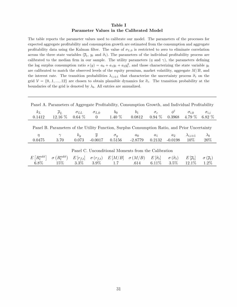
A. Calibration
This subsection describes the parameters chosen to calibrate the model so that it matches
some key features of the data on asset prices, pro¯tability, and consumption. All parame-
ters are summarized in Table I, together with some implied aggregate quantities. We use
data on quarterly real aggregate consumption and aggregate pro¯tability between 1966Q1
and 2002Q1 to estimate the parameters for ct in equation (8) and for ½t in equation (3).
Both series are described in the Appendix. We apply the Kalman ¯lter to the discretized
versions of the processes. The estimated parameters imply expected consumption growth of
2.37% and volatility of 0.94% per year. For pro¯tability, we obtain ½L = 12:16% per year,
kL = 0:1412, and ¾LL = 0:64% per year.11 We set ¾L;0 equal to zero, very close to the
unconstrained estimate, which implies zero correlation between ½t and yt. As a result, all
three state variables that drive IPO volume (½t, yt, and b¾t) are independent of each other.******************** INSERT TABLE I HERE ********************
The agents' preferences are characterized by the processes for st in equation (5), yt in
equation (6), and by the utility parameters ´ and °. The parameters are chosen to match
some basic empirical properties of the market portfolio. Since newly listed ¯rms comprise a
small fraction of the market (e.g., Lamont (2002)), we represent the market by a \long-lived
¯rm" with instantaneous pro¯tability of ½t. The formulas for the long-lived ¯rm's M/B
ratio (Mmt =B
mt ), expected return (¹
mR ), and volatility (¾
mR ) are given in the Appendix. The
preference parameters are chosen to calibrate ¹mR , ¾mR , and M
mt =B
mt to their empirical values
for the market, while producing reasonable properties for the real risk-free rate. Our values
for y and ¾y imply the average equity premium of 6.8% and market volatility of 15% per
year. The speed of mean reversion ky implies a half-life of 9.5 years for yt. The long-lived
¯rm's ratio of dividends to book equity is set to 10% per year, which produces an average
aggregate M/B of 1.7, equal to the time-series average in the data. The average risk-free
rate is 3.3% per year. The volatility of the risk-free rate is 3.9%, which is slightly higher
than in the data (as is common in models with habit utility), but still reasonable.
The parameters for individual ¯rm pro¯tability ½it in equation (1) are chosen to match
the median ¯rm in the data. We use Ái = 0:3968, estimated by P¶astor and Veronesi (2003a),
who also report an 8.34% per year median volatility of the AR(1) residuals for individual ¯rm
pro¯tability. We decompose this volatility into ¾i;0 = 4:79% and ¾i;i = 6:82% per year, which
implies a M/B of 1.7 for a ¯rm with 15 years to patent expiration and bÃit = 0 when b¾t = 0,yt = ¹y, and ½
it = ½t = ½L. Finally, prior uncertainty b¾t moves along the grid V = f0; 1; :::; 12g
11
% per year. The transition probabilities are such that there is 10% probability in any given
month of b¾t moving up or down to an adjacent value in the grid. If b¾t hits the boundary ofthe grid, there is a 20% probability of moving away from the boundary.
The parameters of the IPO timing model are speci¯ed as follows. The proportional un-
derwriting fee is set equal to f = 0:07.12 The lag between the IPO ¯ling and the IPO itself
is set equal to ` = 3 months.13 The capital required for production is assumed to be propor-
tional to the book value of the long-lived ¯rm, Bti = qBmti , with q = 0:0235%.14
B. Simulation Evidence around IPO Waves
Using the parameters from the previous subsection, we simulate our model over a pe-
riod of 10,000 years (120,000 months). One new idea is patented each month, with excess
pro¯tability bÃit drawn randomly from the set f¡6;¡4; : : : ; 4; 6g % per year with equal prob-abilities. Each patent has T = 15 years to expiration.
We de¯ne IPO waves as follows. Following Helwege and Liang (2003), we calculate three-
month centered moving averages in which the number of IPOs in each month is averaged
with the numbers of IPOs in the months immediately preceding and following that month.
We de¯ne \hot markets" as those months in which the moving average falls into the top
quartile across the whole simulated sample. We then de¯ne IPO waves as all sequences of
consecutive hot-market months.15 In our simulated sample, there are 4,116 IPO waves whose
length ranges from one to 17 months, with a median of three months. The maximum number
of IPOs in any given month is 51, the median is one, and the average is 0.9.
Since we assume a three-month lag between an IPO ¯ling and the IPO itself, we also
de¯ne an IPO \pre-wave" as an IPO wave that is shifted back in time by three months.
Each IPO wave in our model is driven by state variable changes that occur in the respective
pre-wave. We let \b" denote the last month before the wave begins, and \e" denote the
last month of the wave. An IPO wave begins at the end of month b and ends at the end of
month e. A pre-wave begins at the end of month b-3 and ends at the end of month e-3.
Table II reports the averages of selected variables around IPO waves. Given the size
of the simulated sample, we can treat all averages as population values, so no p-values are
shown. Column 1 of Panel A reports the average change in the given variable during a
pre-wave. First, IPO waves tend to be preceded by pre-wave declines in expected market
return ¹t, in which the average pre-wave change is -0.99% per year. This decline is due
to both components of ¹t, expected excess return (-0.46%) and the risk-free rate (-0.53%).
Second, expected aggregate pro¯tability ½t rises by 0.06% per year during a pre-wave, on
average. Third, IPO waves are preceded by increases in prior uncertainty b¾t, in which theaverage pre-wave change is 0.33% per year. Table II thus illustrates the importance of all
12
three channels (discount rate, cash °ow, and uncertainty) in generating IPO waves.
******************** INSERT TABLE II HERE ********************
The weakest of the three channels in Table II seems to be the cash °ow channel, for
two reasons. First, ½t exhibits relatively little variation, because aggregate pro¯tability data
that is used to calibrate the process for ½t is relatively stable over time. Second, ½t reverts
to its mean relatively fast (e.g., faster than the variable yt that drives ¹t), so changes in ½t
are perceived as short-lived. The inventor's option to wait for an increase in ½t is thus less
valuable, and ½t has a weaker e®ect on IPO volume than ¹t and b¾t do.IPO waves in our model are caused by changes in market conditions, not levels. Table
II shows that market conditions are typically only slightly more favorable during the waves
than outside the waves. The level of market conditions is re°ected in the aggregate M/B,
de¯ned as the sum of earnings divided by the sum of book values across all ¯rms. M/B rises
during the pre-waves by 0.11 on average, which is consistent with IPO waves being produced
by improvements in market conditions. However, the level of M/B during the waves is only
slightly higher than it is outside the waves (1.78 vs 1.76, on average). The reason is that there
is an interesting path dependence in IPO volume. Improvements in market conditions induce
IPOs, thus depleting the backlog of private ¯rms waiting to go public. After su±ciently large
improvements, there is no backlog left, and IPO volume cannot exceed one per month when
M/B is high. Similarly, the backlog of private ¯rms builds up as market conditions get worse,
and an improvement in unfavorable market conditions can induce much of the large backlog
to go public when M/B is low.
The relation between IPO volume and M/B is illustrated in Figure 4 on a randomly se-
lected 100-year segment of the simulated data. The ¯gure shows dramatic variation in IPO
volume: There are periods as long as six years in which no IPOs take place, but also months
of feverish IPO activity, with over 30 IPOs per month.16 IPO waves invariably occur after
increases in M/B, but not necessarily when M/B is high. Similarly, periods when no ¯rms
go public tend to be preceded by severe drops in M/B.
******************** INSERT FIGURE 4 HERE ********************
B.1. Proxies for Changes in Market Conditions
Changes in market conditions can be observed in our simulated environment, but not in
the data. Therefore, we must construct observable proxies for our empirical analysis.
One key quantity that is unobservable in the data is the expected market return ¹t. Its
risk-free rate component is observable, but the equity premium is not. One proxy for the
13
equity premium is market return volatility (MVOL). This volatility is highly correlated with
the equity premium in our model because both variables decrease with yt in the plausible
range. Based on our long simulated time series, the correlation between MVOL and the
equity premium is 0.90, whereas MVOL's correlations with ½t and b¾t are 0.05 and zero,respectively. All correlations are computed for ¯rst di®erences because those are used in the
empirical work. The second proxy for changes in ¹t is realized market return, motivated by
the fact (e.g., Campbell (1991)) that market returns seem to respond more to news about
discount rates than to news about cash °ows. High realized market returns thus likely re°ect
declines in expected market return, and vice versa. In our simulation, realized market returns
are indeed highly negatively correlated with changes in ¹t (-0.94).
Prior uncertainty b¾t is also unobservable in the data. Both the M/B and the return
volatility of IPOs are strongly positively related to b¾t, but neither the M/B nor the volatilityof the long-lived ¯rm depends on b¾t. This distinction suggests two proxies for b¾t. One proxy,NEWVOLt = ¾ipoR;t ¡ ¾mR;t, compares the return volatilities of IPOs and the long-lived ¯rm.The second proxy compares their M/B ratios: NEWMBt = log
¡M ipot =Bipot
¢¡ log (Mmt =B
mt ).
The intuition that both NEWVOL and NEWMB should increase with b¾t is con¯rmed in ourlong simulated sample. Both proxies have high positive correlations (0.80 and 0.59) with b¾t,but their correlations with the other two state variables are much lower: 0.09 with ¹t and
zero with ½t for NEWVOL, -0.29 with ¹t and 0.09 with ½t for NEWMB. Thus, our proxies
for changes in market conditions have solid theoretical motivation.
Table II examines the variation of these proxies around simulated IPO waves. MVOL
declines during the pre-waves by an average of 0.47% per year, which re°ects a pre-wave
decline in expected market return. NEWVOL and NEWMB both increase during the pre-
waves by 2.34% per year and 0.07, respectively, which re°ects a pre-wave increase in prior
uncertainty.17 Realized market returns should be unusually high before IPO waves, especially
due to declines in expected market return. Indeed, Panel B shows that average return is
signi¯cantly higher during the pre-waves than outside: 40.30% compared to 7.05% per year.
Market returns during IPO waves and in the ¯rst three post-wave months are relatively low,
about 9% for total returns, which is less than the 10.27% average outside a wave. There are
two reasons behind the lower market returns. First, these returns are expected to be low
if the wave is caused by a pre-wave decline in expected return. Second, market conditions
typically begin deteriorating during the wave because of the endogeneity of IPO timing. If
market conditions continued to get better, the wave would likely continue as well.
C. Regression Analysis
Table III analyzes the determinants of IPO volume in a regression framework. Each
14
column reports the coe±cients from a regression of the number of IPOs on the variables
listed in the ¯rst column. All variables are simulated from our calibrated model. Although
the model is simulated at a monthly frequency, all variables are cumulated to the quarterly
frequency so that Table III matches its empirical counterparts, Tables VI and VII. We do not
report any p-values. All coe±cients are highly statistically signi¯cant because the simulated
sample is so large (40,000 quarters).
******************** INSERT TABLE III HERE ********************
We ¯rst examine the discount rate channel. As shown in column 1 of Table III, IPO
volume increases after declines in expected market return over the previous two quarters.
Column 6 shows that IPO volume also increases after declines in the risk-free rate. Column
5 shows that declines in MVOL tend to be followed by more IPOs. The results in column
4 also support the discount rate channel: IPO volume is positively related to past market
returns, but negatively related to future and current returns. Realized returns are high while
the expected market return drops, but they are low after the drop stops.
The cash °ow and uncertainty channels are also supported by Table III. Column 2 shows
that IPO volume is high after increases in ¹½t. IPO volume is also high after increases in prior
uncertainty b¾t, as shown in column 3, as well as after increases in NEWMB and NEWVOL(columns 8 and 9), both of which proxy for b¾t in our empirical work. Moreover, IPO volumeis positively related to the level of M/B in the previous quarter. This relation is signi¯cant
statistically but not economically, as shown in Table II.
To be consistent with the subsequent empirical regressions, all regressions in Table III
include a lag of IPO volume on the right-hand side. This lag is always signi¯cant, but its
removal does not alter any of the relations noted above. When we compare the R2's in the
¯rst three columns, the discount rate channel seems the strongest, and the cash °ow channel
the weakest. The R2's are relatively low, between 0.04 and 0.12, because the true relations
between IPO volume and the given variables are complex and nonlinear. We run linear
regressions to be consistent with our empirical regressions, and also because they su±ce to
demonstrate the presence of all three channels that produce IPO waves in our model.
D. Robustness to Pre-IPO Idiosyncratic Risk
In our model, a private ¯rm's IPO timing decision is driven by the ¯rm's market value,
which varies only with market conditions and with the passage of time (equations 11 and
12). The ¯rm's value does not depend on ¯rm-speci¯c risk, because there is no production
or learning before the IPO. In reality, though, private ¯rms usually do face idiosyncratic
risk, which creates ¯rm-speci¯c reasons for going public. This section explains why the main
15
predictions of our model obtain also in the presence of pre-IPO idiosyncratic risk.
In general, a private ¯rm's decision to go public depends on the ¯rm's own expected
return, its own expected pro¯tability, and its own prior uncertainty. We refer to these three
elements as \¯rm conditions." Firm conditions clearly depend on market conditions. For
example, if expected market return drops, expected individual stock returns must also drop,
on average. In our model, ¯rm conditions for private ¯rms are in fact perfectly correlated
with market conditions, because there is no pre-IPO idiosyncratic risk. The correlation
is lower if such risk is present, which raises the question of whether ¯rm conditions move
together su±ciently to cause IPO waves. Measuring this comovement is di±cult, because ¯rm
conditions are unobservable. Related evidence is provided by Vuolteenaho (2002), who ¯nds
that changes in expected returns are highly correlated across ¯rms and concludes that these
changes are \predominantly driven by systematic, marketwide components." More generally,
the comovement in ¯rm conditions must be signi¯cant because stock prices change if and
only if ¯rm conditions change, and stock prices do exhibit signi¯cant comovement. For
example, of the 17,832 ¯rms with more than three years of data on CRSP between January
1926 and December 2002, 96.2% have positive estimated market betas, and 74.2% of those
betas are statistically signi¯cant. The average R2 from the corresponding monthly market
model regressions is 0.13. Note that for changes in market conditions to a®ect IPO volume,
most of the variation in ¯rm conditions does not need to be common; it is su±cient if a
signi¯cant part of this variation is common.
To analyze theoretically how idiosyncratic risk a®ects IPO waves, we solve a modi¯ed
version of our model in which private ¯rms face idiosyncratic risk due to pre-IPO learning.
We assume that agents observe signals about ¹Ãi before the IPO, so that the perception
of ¹Ãi exhibits ¯rm-speci¯c pre-IPO variation. We simulate the modi¯ed model with signal
precision chosen to make idiosyncratic risk more important than in the data.18 As expected,
the IPO volume in the simulation is less volatile than in our original model. This deviation
from our model is realistic, because IPO volume is more volatile in our model than it is in
the data (cf. Figures 1 and 4). More important, the IPO waves observed in the simulation
have properties very similar to those obtained in our model. The discount rate and cash °ow
channels remain highly signi¯cant in the simulated regressions; only the uncertainty channel
is weaker because higher uncertainty about pre-IPO signals increases the value of the option
to wait (Cukierman (1980)). Therefore, our conclusions also hold in the presence of pre-IPO
idiosyncratic risk. We focus on the simpler framework without pre-IPO learning because
the modi¯ed framework is signi¯cantly more complicated and computationally challenging
without adding any substantial new insights into the time variation in IPO volume.
16
IV. Empirical Analysis
This section empirically investigates the three channels (discount rate, cash °ow, and
uncertainty) through which time-varying IPO volume is created in our model.
A. Data
The data on the number of IPOs, obtained from Jay Ritter's website, cover the period
January 1960 through December 2002. To avoid potential concerns about nonstationarity
(see Lowry (2003)), we de°ate the number of IPOs by the number of public ¯rms at the end
of the previous month.19 In the rest of the paper, \the number of IPOs" and \IPO volume"
both refer to the de°ated series, whose values range from zero to 2.1% per month, with an
average of 0.5%. The pattern of time variation in the de°ated series looks very similar to
the pattern in the raw series plotted in Figure 1.
The data on our proxies for changes in market conditions are also constructed monthly for
January 1960 through December 2002, unless speci¯ed otherwise. We use all data available
to us. Market returns (MKT) are total returns on the value-weighted portfolio of all NYSE,
Amex, and Nasdaq stocks, extracted from CRSP. Market volatility (MVOL) is computed
each month after July 1962 as standard deviation of daily market returns within the month.
The aggregate M/B ratio (M/B), plotted in Figure 5, is the sum of market values of equity
across all ordinary common shares divided by the sum of the most recent book values of
equity. The real risk-free rate (RF) is the yield on a one-month T-bill in excess of expected
in°ation, where the latter is the ¯tted value from an AR(12) process applied to the monthly
series of log changes in CPI from the Bureau of Labor Statistics. Aggregate pro¯tability,
measured as return on equity (ROE), is computed quarterly for 1966Q1 through 2002Q1
using Compustat data, as described in the Appendix. This measure of pro¯tability follows
the de¯nition of ½it in Section I.A. Another measure of cash °ow expectations is the I/B/E/S
summary data on equity analysts' forecasts of long-term earnings growth. These forecasts
have horizons of ¯ve years or more, which makes them suitable, given the relatively long-
term nature of ¹½t. For each ¯rm and each month, the average forecast of long-term earnings
growth is computed across all analysts covering the ¯rm. The forecast of average earnings
growth (IBES) is then computed by averaging the average forecasts across all ordinary com-
mon shares. The resulting series is available for November 1981 through March 2002.
******************** INSERT FIGURE 5 HERE ********************
The proxies for prior uncertainty are constructed as follows. New ¯rm excess volatility
(NEWVOL) in a given month is computed by subtracting market return volatility from the
median return volatility across all new ¯rms, which are de¯ned as those ¯rms whose ¯rst
17
appearance in the CRSP daily ¯le occured in the previous month. A given ¯rm's return
volatility in each month is the standard deviation of daily stock returns within the month.
The variable NEWVOL has 464 valid monthly observations in the 486-month period between
July 1962 and December 2002. New ¯rm excess M/B ratio (NEWMB) is computed for each
month between January 1950 and March 2002 as follows. First, we compute the median
M/B across all new ¯rms, which are de¯ned as ¯rms that appeared in the CRSP monthly
¯le in the previous year.20 The variable NEWMB is computed as the natural logarithm of
that median minus the log of the median M/B across all ¯rms. The construction of M/B
for individual ¯rms is described in the Appendix. The variable NEWMB has eight missing
values between January 1960 and March 2002. The monthly time series of NEWVOL and
NEWMB are plotted in Figure 6.
******************** INSERT FIGURE 6 HERE ********************
Figure 6 shows that both NEWMB and NEWVOL rise sharply in the late 1990s and
decline after 2000. The variable NEWVOL exhibits a remarkable pattern: In 1998, it triples
from about 2% per day to about 6%, it remains around 6% through the end of 2000, and
then it drops back to about 2% after 2000. Prior uncertainty was apparently unusually high
in 1998 through 2000. This fact is not surprising, since long-term prospects of new ¯rms are
particularly uncertain when new paradigms are being embraced. The high prior uncertainty
may have induced many ¯rms to go public in the late 1990s, and it might also have con-
tributed to the high valuations of many IPOs at that time.
B. Empirical Evidence around IPO Waves
Between January 1960 and December 2002, there are 16 IPO waves. Their lengths range
from one to 21 months, with a median of ¯ve months. Some summary statistics for the 16
waves are shown in Tables IV and V. All variables except for the unitless M/B and NEWMB
are in percent per year. In Table IV, all but three waves are preceded by above-average
market returns during the pre-wave, as predicted by the model. Only one (one-month) wave
is preceded by a negative return. For all but two waves,MVOL declines during the pre-wave,
which is consistent with a pre-wave decline in expected market return. The wave that begins
in 1993 appears to be due to the cash °ow channel. The waves in 1991, 1992, and especially
1999 are preceded by increases in both NEWVOL and NEWMB, suggesting that these waves
may have been caused at least in part by increases in prior uncertainty.
******************** INSERT TABLE IV HERE ********************
18
Table V reports variable averages across the 16 waves. The t-statistics, given in paren-
theses, measure the signi¯cance of the di®erence between the averages within and outside
the given period. For example, the t-statistic for average MVOL during a wave (-3.18) is
computed by regressing MVOL on a dummy variable equal to one if the month is part of an
IPO wave, and zero otherwise. A positive (negative) t-statistic indicates that the variable's
average in the given period is bigger (smaller) than the average in the rest of the sample.
******************** INSERT TABLE V HERE ********************
The average pre-wave change in MVOL is signi¯cantly negative at -2.81% (t = ¡2:27),which is consistent with IPO waves being caused by declines in expected market return. The
values ofM/B, ROE, and IBES all increase before the waves, as the model predicts, but these
increases are statistically insigni¯cant. The value of NEWVOL increases signi¯cantly during
pre-waves (t = 2:27), consistent with the uncertainty channel, but the value of NEWMB
does not. The value of RF increases insigni¯cantly during pre-waves, contrary to our model,
which predicts a pre-wave decrease. Panel B shows that average market returns are high
before IPO waves (e.g., 31.17% annualized with t = 2:77 two quarters before a wave), as
predicted by the model. Market returns are low during and especially after IPO waves, but
they are not signi¯cantly lower than in the rest of the sample. The return pattern is similar
to the model-predicted pattern observed in Table II.
Since the averages in Table V are computed across only 16 IPO waves, only a few rela-
tions are statistically signi¯cant. More detailed empirical analysis is therefore performed in
the following section, which focuses on IPO volume rather than on IPO waves alone.
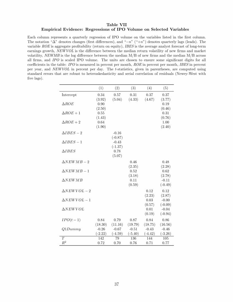
C. Regression Analysis
Each column in Tables VI and VII corresponds to a separate regression, in which the
number of IPOs in the current quarter is regressed on proxies for changes in market condi-
tions. Lagged IPO volume is included on the right-hand side to capture persistence in IPO
volume that is unexplained due to any potential misspeci¯cation in the regressions. Lowry
(2003) also includes lagged IPO volume on the right-hand side of her regressions. She also
always includes a ¯rst-quarter dummy that captures the apparent seasonality in IPO volume,
and we follow her treatment. Both variables are signi¯cant in each regression.
******************** INSERT TABLE VI HERE ********************
******************** INSERT TABLE VII HERE ********************
First, we test the discount rate channel, in which IPOs are triggered by declines in
19
expected market return. Column 1 of Table VI shows that IPO volume is positively related
to total market returns over the previous two quarters (t = 3:34 and 3.25), which is consistent
with both the discount rate and cash °ow channels. Moreover, IPO volume is negatively
related to market returns in the subsequent quarter (t = ¡2:23), which is consistent withthe discount rate channel. This negative relation is also reported by Lamont (2002), Schultz
(2003), and Lowry (2003). The relation with current returns is positive, not negative as in
Table III, but this di®erence does not contradict the model. IPO waves in the data tend to
last longer than our simulated IPO waves, so the actual IPO waves have more overlap than
the simulated waves with the declines in expected market return that caused the waves and,
therefore, also with high realized returns. Column 2 shows that IPO volume is negatively
related to current (t = ¡4:41) as well as past (t = ¡3:59) changes in market volatility, whichis again consistent with the discount rate channel. In column 3, changes in the risk-free rate
are positively related to future IPO volume, not negatively as the model predicts. Combined
with the results in columns 1 and 2, this positive relation suggests that IPO volume is
strongly negatively related to recent changes in the equity premium.
Second, the cash °ow channel is also supported by the data. Column 1 of Table VII
shows that IPO volume is positively related to current (t = 2:50) as well as future changes
in aggregate pro¯tability, which suggests that ¯rms go public when cash °ow expectations
improve. Column 2 reaches the same conclusion. IPO volume is higher (t = 5:07) when
equity analysts upgrade their forecasts of long-term earnings growth.
Third, prior uncertainty also seems to go up before ¯rms go public. In columns 3 and 4
of Table VII, IPO volume is positively related to recent changes in the excess M/B ratio of
new ¯rms (t = 3:18 and 2.35), as well as to recent changes in the excess volatility of new
¯rms (t = 2:23), both of which comove with prior uncertainty in our model.
Some of the proxies for changes in market conditions lose their statistical signi¯cance
when realized market returns are included in the regression. The reason goes beyond the
simple lost-degrees-of-freedom e®ect. In reasonably e±cient markets, prices re°ect much
of the available information, and realized market returns are the best proxy for changes in
market conditions; i.e., when market conditions improve, prices go up, and vice versa. Thus,
it is not surprising that including market returns drives some of the weaker proxies below
the threshold of signi¯cance. The role of these other proxies is only to provide additional
evidence on the likely causes of the observed price changes.
The regressors in Tables VI and VII represent changes in market conditions, whereas the
regressand is the level of IPO volume. Regressing levels on changes is appropriate because
the level of IPO volume is driven by changes in market conditions in our model. Lowry
(2003), who uses the same dependent variable as we do, also suggests using changes in the
number of IPOs as a way of avoiding nonstationarity. Using this rede¯ned dependent vari-
20
able leads to results that are almost identical to those reported here.
D. Rational vs. Irrational IPO Waves
Many recent studies blame time-varying IPO volume on market ine±ciency, arguing that
IPO volume is high when shares are overvalued. In this section, we examine the extent to
which our empirical evidence is consistent with the simple behavioral story in which ¯rms
go public to take advantage of irrational overpricing.
In the mispricing story, IPO volume is high when the market is overvalued. Under the
common behavioral assumption that misvaluation is re°ected in M/B, this story predicts a
positive relation between IPO volume and the level of aggregate M/B. Our rational model
also predicts a positive relation (see Table III), but a weak one (see Table II), because IPO
volume in our model is driven mainly by changes in market conditions, not levels. Column
4 of Table VI shows that IPO volume is not signi¯cantly related to the level of aggregate
M/B at the end of the previous quarter.21 Column 5 presents a horserace between the levels
and changes, in that IPO volume is regressed on M/B as well as on market returns. In this
regression, market returns remain highly signi¯cant and M/B remains insigni¯cant. That is,
IPO volume is high after a run-up in stock prices, but not necessarily when the level of prices
is high. This evidence, which ¯ts the intuition described in Section III, provides additional
support for our model, but not for the overvaluation story.
Neither can our evidence related to the cash °ow channel be easily explained by the
mispricing story. One of our proxies for expected cash °ow, IBES, might be subject to be-
havioral biases if analyst forecasts are biased. However, consider our second proxy, aggregate
pro¯tability (ROE). Column 1 of Table VII shows that IPO volume is positively related to
current and future changes in ROE. This relation is not predicted by the mispricing story,
in which IPO decisions do not re°ect rational expectations of future cash °ows.
The mispricing story also cannot fully explain our results related to the uncertainty
channel. One proxy for prior uncertainty, NEWMB, can be subject to behavioral biases if
we accept the idea that new ¯rms can be more overvalued than seasoned ¯rms. However, it
is not obvious how the mispricing story could justify our result that IPO volume is positively
related to changes in our second proxy, NEWVOL. Mispricing might a®ect the price level,
but it is not clear why it should a®ect the return volatility of new ¯rms.
Nor can the mispricing story account for all of our evidence related to the discount rate
channel. One of our proxies for changes in expected market return, MKT, might be biased
due to mispricing, but it is not clear why our second proxy, MVOL, should be biased. In
the mispricing story, expected market return is driven by investor sentiment, and there is
no obvious reason for market volatility to be related to investor sentiment. Therefore, the
21
mispricing story does not explain why IPO volume is signi¯cantly related to changes in
MVOL in column 2 of Table VI. In summary, four of our empirical ¯ndings are consistent
with our rational model, but they are not predicted by the mispricing story.
V. IPOs and Investment
This section examines the important role of investment in our model. The model features
a link between a ¯rm's decisions to go public and to invest. We discuss the plausibility of
such a link, pointing to ¯rm-level evidence on the extent to which IPO proceeds are invested,
as well as to some evidence on the relation between IPO volume and investment in aggregate.
We also discuss the relation between aggregate investment and market conditions.
The main purpose of an IPO in our model is to raise capital for investment. This
description applies only to a subset of the observed IPOs, because many real-world IPOs
happen for reasons other than investment, such as re¯nancing. However, as long as some
¯rms go public to raise funds for investment, IPO volume should be a®ected by market
conditions. Many ¯rms indeed appear to invest their IPO proceeds. Mikkelson et al. (1997)
report that 64% of the ¯rms going public state in their o®ering prospectus that the reason
for their IPO is to ¯nance capital expenditures. Moreover, Jain and Kini (1994) report that
the capital expenditures of IPOs grow by 142% in the two years around the IPO, on average,
which signi¯cantly exceeds the contemporaneous investment growth for industry-matched
seasoned ¯rms. In fact, the industry-adjusted growth rate in the capital expenditures of
¯rms going public is as large as 109% over the two-year period. Therefore, a link between
the decisions to go public and to invest seems reasonable.22
The link between IPOs and investment seems present also in the aggregate data. Using
data on real private nonresidential ¯xed investment between 1947 and 2002, obtained from
the Bureau of Economic Analysis (BEA), we ¯nd that aggregate investment growth is sig-
for capital to be a key empirical determinant of IPO volume, further supporting the link
between IPOs and investment. Lowry also reports that the total amount raised in the IPOs
is more volatile than the total amount invested, which is precisely what our model predicts.
In our model, the ¯rm invests only part of the IPO proceeds; the rest goes to the inventor as
compensation for the patent, to pay for the inventor's pre-IPO consumption. The variation
in IPO proceeds therefore exceeds the variation in the amount invested. The IPO decision
is often de-linked from the investment decision in the leading explanations for IPO volume,
such as market mispricing and asymmetric information, but the link is essential to obtaining
the relation between IPO volume and market conditions documented in this paper.
Our focus is on IPO waves, but our model can also address a broader issue of cyclicality
of investment. A public ¯rm solving for the optimal time to make an irreversible invest-
22
ment is considering tradeo®s similar to those of our inventor, and \investment waves" might
develop after market conditions improve. Consistent with this idea, several studies (e.g.,
Barro (1990), and Baker et al. (2003)) report a positive relation between investment and
stock prices. Using the BEA data, we ¯nd that investment growth is positively related to
recent market returns and negatively related to future market returns. Investment growth
is also positively related to current and future changes in aggregate ROE. We conclude that
aggregate investment is related to changes in market conditions, similar to IPO volume.
These results suggest that our model makes useful predictions not only for IPO volume,
but also for aggregate investment. At the same time, we believe that our model is better
suited for studying investment by new ¯rms than for examining investment by public ¯rms,
for several reasons. First, public ¯rms often invest simply to maintain a competitive stock
of physical capital, rather than to embark on new projects with uncertain and perishable
abnormal pro¯ts. This fact makes some features of our framework, such as prior uncertainty,
less relevant for public ¯rms. Indeed, aggregate investment growth seems unrelated to our
proxies for prior uncertainty in the data. Second, the investment decisions of public ¯rms
may be a®ected by the ¯rms' existing projects, a complication that is absent from our
model in which inventors have only one project at a time. Third, we assume that learning
about Ãistarts when the production begins, which seems to better describe IPOs of start-up
companies than investment by public ¯rms. Learning about a public ¯rm's new project
can take place before the production begins, because investors can observe the ¯rm's other
projects, whose payo®s are presumably correlated with the new project's payo®s.
In addition, focusing on IPOs rather than on aggregate investment preserves market
completeness. New projects introduce new idiosyncratic risk (Wi;t) in the economy. This risk
is not spanned by the existing securities, so markets become incomplete unless a new security
is issued that can perfectly hedge the new risk. Markets are dynamically complete in our
model because each new project is accompanied by an issue of a claim on the project's cash
°ow. This issue has a natural interpretation as an IPO of a start-up company. The equity
issued in the IPO provides a perfect hedge for the new project because it is a claim on that
project only. In contrast, investments by public ¯rms are not accompanied by issues of equity
that would provide a perfect hedge. For example, the equity issued in an SEO is a claim to
all projects of this public ¯rm, not just the new project. Due to market incompleteness in
that case, the SDF may not be unique, which could complicate the analysis.
VI. Conclusion
In their survey of the IPO literature, Ritter and Welch (2002) conclude that \market
conditions are the most important factor in the decision to go public." We agree, and we
point out three dimensions of market conditions that appear especially relevant. Ritter
23
and Welch also state that \perhaps the most important unanswered question is why issuing
volume drops so precipitously following stock market drops." Our paper provides a simple
answer. When market conditions worsen, stock prices drop and IPO volume declines because
private ¯rms choose to wait for more favorable market conditions before going public.
This answer is only one of many testable implications of our model of optimal IPO timing.
We show by simulation that the model also implies that IPO waves should be preceded
by high market returns, followed by low market returns, and accompanied by increases in
aggregate pro¯tability. In addition, IPO waves should be preceded by an increased disparity
between new ¯rms and old ¯rms in terms of their valuations and return volatilities. IPO
volume should be related to changes in stock prices, but less so to their levels. All of these
implications are con¯rmed in the data.
Some implications of our model, such as the low post-wave market returns, are also
consistent with the behavioral story in which ¯rms go public in response to market over-
valuation. However, several of our empirical ¯ndings are not predicted by this behavioral
story. For example, this story does not predict that IPO volume should be related to recent
changes in market return volatility or positively related to changes in aggregate pro¯tability.
Behavioral biases have also been blamed for the high IPO valuations observed in the
late 1990s, but those valuations need not have been irrational. IPO valuations in our model
tend to be relatively high, partly because IPO timing is endogenous and partly due to prior
uncertainty about the average future pro¯tability of IPOs. According to its proxies, prior
uncertainty was unusually high in the late 1990s. This high prior uncertainty may have
attracted many ¯rms to go public, and it might also have contributed to the high valuations
of many IPOs at that time.
Many IPOs in the 1990s happened in technology-related industries. Industry clustering of
IPOs obtains in a minor extension of our model. Instead of assuming that prior uncertainty
is the same for all ¯rms, we can assume that this uncertainty is more similar for ¯rms in the
same industry. Average excess pro¯tability is also likely to be more correlated across ¯rms in
the same industry. Increases in industry-speci¯c prior uncertainty or industry-speci¯c excess
pro¯tability can lead to IPO waves concentrated in the given industry, without triggering
IPOs in other industries. These implications can be tested empirically in future work.
Future research can also endogenize the innovation process. We assume that new ideas
arrive at a constant pace, but if capital must be raised to produce an idea, then low cost of
capital might accelerate innovation, leading to more ideas and more IPOs. High expected
aggregate pro¯tability might also speed up innovation and produce more IPOs. These e®ects,
if present, would link IPO volume more closely to the level of market conditions, and they
would also amplify the variation in IPO volume obtained in our model.
24
1960 1965 1970 1975 1980 1985 1990 1995 20000
20
40
60
80
100
120
140
Year
Numb
er of
IPOs
Figure 1. IPO volume. The ¯gure plots the number of IPOs in each month betweenJanuary 1960 and December 2002. The data is obtained from Jay Ritter's website.
25
t i
idea is patented
τ i
IPO time
T i
patent expires
t
h i = time to expiration
decision to go public istaken
τ i + l
Figure 2. The timing of events in our model. At time ti, an idea is patented by aninventor. The patent expires at time Ti. The inventor chooses whether to go public, and ifso, when. If the inventor decides to go public at time ¿i, the IPO takes place at time ¿i + `.
26
0 0.05 0.1 0.15 0.20.06
0.08
0.1
0.12
0.14
0.16
0.18
0.2Panel A. T = 15, ψ = 0
Exp
. agg
. pro
fitab
ility
( ρ t )
|
σ=0 σ=.05σ=.1
0 0.05 0.1 0.15 0.20.06
0.08
0.1
0.12
0.14
0.16
0.18
0.2Panel B. T = 15, σ = 0
Exp
. agg
. pro
fitab
ility
( ρ t )
|
ψ=−.04ψ=0 ψ=.04
0 0.05 0.1 0.15 0.20.06
0.08
0.1
0.12
0.14
0.16
0.18
0.2Panel C. ψ = 0, σ = 0
Expected market return ( µt )
Exp
. agg
. pro
fitab
ility
( ρ t )
|
T=15T=10T=5
0 0.05 0.1 0.15 0.20.06
0.08
0.1
0.12
0.14
0.16
0.18
0.2Panel D. ψ = 0, σ = 0
Expected market return ( µt )
Exp
. agg
. pro
fitab
ility
( ρ t )
|
T=2 T=1.5T=1
Figure 3. Optimal IPO timing. Each panel plots the entry boundary; i.e., the setof pairs of expected market return (horizontal axis) and expected aggregate pro¯tability(vertical axis) that trigger the decision to go public. An IPO takes place in the parameterregion northwest of each boundary. The entry boundaries are reported for three levels ofprior uncertainty b¾t per year (Panel A), ¯rm-speci¯c excess pro¯tability Ã̂ per year (PanelB), and time to the patent's expiration in years (Panels C and D).
27
0 10 20 30 40 50 60 70 80 90 1000
5
10
15
20
25
30
35Panel A. Simulated IPO Volume
Num
ber o
f IPO
s
0 10 20 30 40 50 60 70 80 90 1000.5
1
1.5
2
2.5Panel B. Simulated Aggregate Market−to−Book Ratio
M/B
Year
Figure 4. Simulated IPO waves. The ¯gure plots the monthly number of IPOs and theaggregate M/B ratio in a randomly selected 100-year segment of our simulated data. AllIPOs are optimally timed in the sense of Section II. The aggregate M/B ratio is de¯ned asthe sum of earnings divided by the sum of book values across all ¯rms in the simulation.
28
1960 1965 1970 1975 1980 1985 1990 1995 20000.5
1
1.5
2
2.5
3
3.5
4
M/B
Figure 5. Monthly time series of the aggregate market-to-book ratio. Each month,the aggregate market-to-book ratio (M/B) is computed as the sum of market values of equityacross all ¯rms divided by the sum of the most recent book values of equity.
29
1960 1965 1970 1975 1980 1985 1990 1995 20000
2
4
6
8
10%
per
day
Panel A. New Firm Excess Volatility (NEWVOL)
1960 1965 1970 1975 1980 1985 1990 1995 2000−0.5
0
0.5
1
1.5
2
Year
Log
diffe
renc
e
Panel B. New Firm Excess M/B (NEWMB)
Figure 6. Monthly time series of proxies for prior uncertainty. Panel A plotsNEWVOL, the median return volatility (standard deviation of daily returns) across all newlylisted ¯rms in excess of market return volatility. The values of NEWVOL are availablebetween July 1962 and December 2002. Panel B plots NEWMB, the log median M/B acrossall newly listed ¯rms in excess of the log median M/B across all ¯rms. The values of NEWMBare available between January 1960 and March 2002.
30
Table IParameter Values in the Calibrated Model
The table reports the parameter values used to calibrate our model. The parameters of the processes for
expected aggregate pro¯tability and consumption growth are estimated from the consumption and aggregate
pro¯tability data using the Kalman ¯lter. The value of ¾L;0 is restricted to zero to eliminate correlation
across the three state variables (½t, yt and b¾t). The parameters of the individual pro¯tability process arecalibrated to the median ¯rm in our sample. The utility parameters (´ and °), the parameters de¯ning
the log surplus consumption ratio s (y) = a0 + a1yt + a2y2t , and those characterizing the state variable yt
are calibrated to match the observed levels of the equity premium, market volatility, aggregate M=B, and
the interest rate. The transition probabilities ¸i;i§1 that characterize the uncertainty process b¾t on thegrid V = f0; :1; :::; :12g are chosen to obtain plausible dynamics for b¾t. The transition probability at theboundaries of the grid is denoted by ¸b. All entries are annualized.
Panel A. Parameters of Aggregate Pro¯tability, Consumption Growth, and Individual Pro¯tability
Panel B. Parameters of the Utility Function, Surplus Consumption Ratio, and Prior Uncertainty
´ ° ky y ¾y a0 a1 a2 ¸i;i§1 ¸b0.0475 3.70 0.073 -0.0017 0.5156 -2.8779 0.2132 -0.0198 10% 20%
Panel C. Unconditional Moments from the Calibration
E£Rmktt
¤¾¡Rmktt
¢E [rf;t] ¾ (rf;t) E [M=B] ¾ (M=B) E [b¾t] ¾ (b¾t) E [½t] ¾ (½t)
6.8% 15% 3.3% 3.9% 1.7 .614 6.11% 3.5% 12.1% 1.2%
31
Table IISimulation Evidence Around IPO Waves
The table reports averages of selected variables and market returns around simulated IPO waves. \b" standsfor the beginning of an IPO wave, i.e., the end of the last month before the wave begins. \e" stands for theend of the wave's last month. \b(e)§n" denotes n months before or after the beginning (end) of a wave. Apre-wave is de¯ned as the period that begins at the end of month b{3 and ends at the end of month e{3.Expected excess and total returns are computed for the market portfolio, the value-weighted portfolio of allexisting simulated ¯rms. Expected pro¯tability stands for ½, and prior uncertainty stands for b¾. The variableMVOL is market return volatility, RF is the risk-free rate, M/B is the aggregate M/B ratio, NEWVOL isthe di®erence between the return volatility of a new ¯rm and market volatility, and NEWMB is the logdi®erence between the M/B of a new ¯rm and the M/B of the market. All variables except for M/B andNEWMB are expressed in percent per year.
Panel A. Averages of ¯rst-column variables
Avg change Before wave Wave After wave Outsidein pre-wave b-6 b-3 b b+1:e e e+3 e+6 wave
Table IIISimulation Evidence: Regressions of IPO Volume on Selected Variables
Each column represents a quarterly regression of IPO volume on the variables listed in the ¯rst column.All variables are taken from a 10,000-year-long sample simulated from our calibrated model. No t-statisticsare given because all reported numbers are highly signi¯cant. The notation \¢" denotes changes (¯rstdi®erences), and \¡n" (\+n") denotes quarterly lags (leads). The notation ER denotes expected totalmarket return, MKT is realized market return, MVOL is market return volatility, RF is the risk-free rate,M/B is the aggregate M/B ratio, NEWMB is the log di®erence between the M/B of a new ¯rm and the M/Bof the market, NEWVOL is the di®erence between the return volatility of a new ¯rm and market volatility,and IPO is the number of ¯rms that went public this quarter. The units are chosen to ensure some signi¯cantdigits for all coe±cients in the table: MKT is measured in decimals per month, and all other variables exceptfor the unitless M/B and NEWMB are in percent per year.
The table reports some summary statistics for the 16 IPO waves observed in our sample period of January 1960 throughDecember 2002. \Avg pre-wave market return" for a given wave denotes the average monthly total market return during therespective pre-wave. The variable MVOL is market return volatility, M/B is the aggregate M/B ratio, RF is the risk-free rate,ROE is aggregate pro¯tability (return on equity), IBES is the average analyst forecast of long-term earnings growth, NEWVOLis the di®erence between the median return volatility of new ¯rms and market volatility, and NEWMB is the log di®erencebetween the median M/B of new ¯rms and the median M/B across all ¯rms. All variables except for M/B and NEWMB areexpressed in percent per year. The values that are not available due to missing data are denoted by \n/a."
Beginning End Number Avg pre-wave Pre-wave change in
of wave of wave of IPOs market return MVOL M/B RF ROE IBES NEWVOL NEWMB
The table reports averages of selected variables and market returns around IPO waves. \b" stands for thebeginning of an IPO wave; i.e., the end of the last month before the wave begins. \e" stands for the endof the wave's last month. \b(e)§n" denotes n months before or after the beginning (end) of a wave. Apre-wave is de¯ned as the period that begins at the end of month b{3 and ends at the end of month e{3.The variable MVOL is market return volatility, M/B is the aggregate M/B ratio, RF is the risk-free rate,ROE is aggregate pro¯tability (return on equity), IBES is the average analyst forecast of long-term earningsgrowth, NEWVOL is the di®erence between the median return volatility of new ¯rms and market volatility,and NEWMB is the log di®erence between the median M/B of new ¯rms and the median M/B across all¯rms. All variables except forM/B and NEWMB are expressed in percent per year. The t-statistics, reportedin parentheses, assess the signi¯cance of the di®erence between the given variable's averages in the givenperiod and outside that period.
Panel A. Averages of selected variables
Avg change Before wave Wave After wave Outsidein pre-wave b-6 b-3 b b+1:e e e+3 e+6 wave
Table VIEmpirical Evidence: Regressions of IPO Volume on Selected Variables
Each column represents a quarterly regression of IPO volume on the variables listed in the ¯rst column.The notation \¢" denotes changes (¯rst di®erences), and \¡n" (\+n") denotes quarterly lags (leads). Thevariable MKT is realized market return, MVOL is market return volatility, RF is the real risk-free rate, M/Bis the aggregate M/B ratio, and IPO is scaled IPO volume. The units are chosen to ensure some signi¯cantdigits for all coe±cients in the table: IPO is measured in percent per month, MKT in decimals per month,MVOL in percent per day, and RF in percent per month. The t-statistics, given in parentheses, are computedusing standard errors that are robust to heteroskedasticity and serial correlation of residuals (Newey-Westwith ¯ve lags).
Table VIIEmpirical Evidence: Regressions of IPO Volume on Selected Variables
Each column represents a quarterly regression of IPO volume on the variables listed in the ¯rst column.The notation \¢" denotes changes (¯rst di®erences), and \¡n" (\+n") denotes quarterly lags (leads). Thevariable ROE is aggregate pro¯tability (return on equity), IBES is the average analyst forecast of long-termearnings growth, NEWVOL is the di®erence between the median return volatility of new ¯rms and marketvolatility, NEWMB is the log di®erence between the median M/B of new ¯rms and the median M/B acrossall ¯rms, and IPO is scaled IPO volume. The units are chosen to ensure some signi¯cant digits for allcoe±cients in the table: IPO is measured in percent per month, ROE in percent per month, IBES in percentper year, and NEWVOL in percent per day. The t-statistics, given in parentheses, are computed usingstandard errors that are robust to heteroskedasticity and serial correlation of residuals (Newey-West with¯ve lags).
Aggregate quarterly consumption data is obtained from NIPA. Consumption is de¯ned asreal per capita consumption expenditures on nondurables plus services, seasonally adjusted.The series is de°ated by the personal consumption expenditure de°ator (PCE), also takenfrom NIPA.The following data is obtained from CRSP and Compustat. Quarterly aggregate prof-
itability (ROE) is computed as the sum across stocks of earnings in the current quarterdivided by the sum of book values of equity at the end of the previous quarter. Quarterlyearnings, which are generally available from 1966Q1, denote income before extraordinaryitems available for common (Compustat item 25) plus deferred taxes from the income ac-count (item 35, if available). If either value is indicated as .A (annual) or .S (semi-annual) inthe quarterly ¯le, these values are divided by four (if .A) or two (if .S). When quarterly bookequity is missing, it is replaced with the most recent annual book equity. Following Famaand French (1993), annual book equity is constructed as stockholders' equity plus balancesheet deferred taxes and investment tax credit (item 35) minus the book value of preferredstock. Depending on availability, stockholder's equity is computed as Compustat item 216, or60+130, or 6-181, in that order, and preferred stock is computed as item 56, or 10, or 130, inthat order. Quarterly book equity, which is generally available from 1972Q1, is constructedanalogously. Stockholders' equity is item 60, or 59+55, or 44-54, preferred stock is item 55,and deferred taxes and tax credit is item 52. If the quarterly values are indicated as .A(annual) or .S (semi-annual) in the SAS data¯le, the respective annual or semiannual valuesare used. Monthly ROE values are interpolated from quarterly values. Market equity iscomputed monthly by multiplying the common stock price by common shares outstanding,both obtained from CRSP. M/B ratio is computed as market equity divided by book equityfrom the most recent quarter. We eliminate the values of market equity and book equitysmaller than $1 million, as well as M/B ratios smaller than 0.01 and larger than 100. Allvariables that require Compustat data (e.g. ROE, M/B) are constructed through the end of2002Q1.
Appendix B: Preferences and the Stochastic Discount Factor
This appendix describes the properties of the process of log surplus consumption
log (St) ´ st ´ s (yt) = a0 + a1yt + a2y2t : (A1)
The process for yt implies a normal unconditional distribution for yt with mean y and variance¾2y=2ky. Let yD = y¡4¾y=
p2ky and yU = y+4¾y=
p2ky be the boundaries between which yt
lies 99.9% of the time. To ensure that log surplus st conforms to the economic intuition of ahabit formation model, we impose the following parametric restrictions: a2 < 0, a1 > ¡2a2yUand a0 < 1=4 (a
21=a2) : These restrictions ensure that for all t, st < 0, and thus St 2 (0; 1),
and that s (y) is increasing in y for all y 2 [yD; yU ]. Log surplus follows the processdst = ¹s (y) dt+ ¾s (y) dW0;t; (A2)
The restrictions above imply that ¾s (y) is positive and decreasing in y, for all y 2 [yD; yU ].Since s increases with y in the relevant range, surplus is perfectly correlated with innovationsto aggregate consumption, and its volatility is higher for low surplus levels.Given the dynamics of consumption in equation (8) and surplus in equation (A2), the
process for the stochastic discount factor ¼t = UC (Ct; Xt; t) = e¡´t (CtSt)
¡° = e¡´t¡°(ct+st)
is given byd¼t = ¡rt¼tdt¡ ¼t¾¼;tdW0;t; (A3)
wherert = R0 +R1½t +R2yt +R3y
2t (A4)
with
R0 = ´ + °b0 + °a1kyy ¡ 12°2¾2c + (°a2 ¡
1
2°2a21)¾
2y ¡ °2a1¾c¾y
R1 = °b1
R2 = °¡2a2kyy ¡ a1ky ¡ °a2
¡2¾c¾y + 2a1¾
2y
¢¢R3 = 2a2°
¡¡ky ¡ °a2¾2y¢and
¾¼;t = ° (¾c + (a1 + 2a2yt) ¾y) : (A5)
The parameter restrictions imposed earlier imply that ¾¼;t decreases as yt (and hence alsothe surplus St) increases. As a result, expected returns and return volatility are low whenyt is high.
Appendix C: Learning
LEMMA 1: Suppose the prior of Ãiat time t0 is normal, Ã
i » N³bÃit0 ; b¾2t0´, and the priors
are uncorrelated across ¯rms. Let It denote the set of ¯rms that are alive at time t. Thenthe posterior of Ã
iat any time t > t0 conditional on Ft = f(½js; cs; ½s) : t0 · s · t; j 2 Itg is
also normal, ÃijFt » N
³bÃit; b¾2i;t´, where(a) The mean squared error b¾2i;t = E ·³Ãi ¡ bÃit´2 jFt¸ is nonstochastic and given by
b¾2i;t = 1
1b¾2t0 + (Ái)2
¾2i;i(t¡ t0)
: (A6)
We note that the uncertainty about Ãideclines deterministically over time due to
learning.
(b) The conditional mean bÃit = E[ÃitjFt] evolves according to the processdbÃit = b¾2i;t Ái¾i;idfWi;t; (A7)
where fWi;t is the idiosyncratic component of the Wiener process capturing the agents'perceived expectation errors (see equation (A8) below).
39
Proof : Consider the vector Zt = (ct; ½t; ½1t ; :::; ½
nt ) of signals to identify the unobservable
variables, stacked in another vector à = (Ã1; :::; Ã
1CCCCA :Proof : From the de¯nition of the vector Yt, we have
dYt = (AY +BYYt) dt+§Y;tdfWt:
The Feynman-Kac theorem implies that H (Yt; t) from (A9) solves the partial di®erentialequation
@H
@t+
5Xi=1
µ@H
@Yi
¶[AY +BYYt]i +
1
2
5Xi=1
5Xj=1
@2H
@Yi@Yj
£§Y;t§
0Y;t
¤ij= ´H (A13)
subject to the boundary condition
H (YT ; T ) = g (YT ) : (A14)
It is easy to verify that the exponential quadratic function (A9) indeed satis¯es (A13) sub-ject to (A14), as long as K0 (t;T ) ; K (t;T ) ; and K6 (t;T ) are the solutions to the systemof ODEs in (A10) through (A12) under the ¯nal conditions presented in the claim of theLemma.¥
PROPOSITION 1: Let hi = Ti ¡ t be the time to expiration of the patent of public ¯rm i.Then(a) The ¯rm's ratio of market value of equity to book value of equity is given by
it;bÃit´ is the vector of state variables characterizing ¯rm i, Q0 ¡hi; b¾2i;t¢ =
K0 (Ti ¡ hi;Ti), Q1 (hi) = K2 (Ti ¡ hi;Ti) + °a1, Qi (hi) = Ki+1 (Ti ¡ hi;Ti) for i =2; ::; 4, Q5 (hi) = K6 (Ti ¡ hi;Ti) + °a2, and Ki (:;Ti)
0 are given in Lemma 2 for theparameterization ³0 = ³2 = 0 and ³1 = v = 1. Analytical, although rather complicated,formulas for these functions are available in P¶astor and Veronesi (2003b).
(b) The ¯rm's excess stock returns follow the process
dRit = ¹iR (yt; hi) dt+ ¾
iR;0 (yt; hi) d
fW0;t + ¾iR;L (hi) d
fWL;t + ¾iR;i (b¾i;t; hi) dfWi;t; (A16)
where dfWj;t's are the Wiener processes given in equation (A8), and
Note: It can be shown that the ¯rm's M/B is increasing in b¾2i;t. Inspection of the ODEsin equations (A10) through (A12) shows that b¾2i;t enters only the ODE de¯nining K0 andhence only Q0 and no other Qi's. Q0 is increasing in b¾2i;t, so that the ¯rm's M/B is increasingin b¾2i;t as well. This fact is shown more explicitly in P¶astor and Veronesi (2003b).Proof : From the pricing formula and Lemma 2:
M it = ¼
¡1t Et
£¼TiB
iTi
¤= e°ct+°a1yt+°a2y
2tEt
he¡´(Ti¡t)eb
iTi¡°cTi¡°a1yTi¡°a2y2Ti
i= e°ct+°a1yt+°a2y
2tH (Yt; t) :
Since BY has only zeros in its ¯rst column, we have£K (t;Ti)
0 ¢BY¤1= 0 in equation (A11).
This implies dK1(t;Ti)dt
= 0 and thus K1 (t;Ti) = 1 for t · Ti: By substituting in H (Yt; t), weobtain
M it = e
°ct+°a1yt+°a2y2t £H (Yt; t) = Bit £ e°a1yt+°a2y
2t £ eK0(t;Ti)+
P5i=2Ki(t;Ti)Yi;t+K6(t;Ti)Y
22;t :
This expression leads immediately to claim (a) on rede¯nition of variables. The proof ofclaim (b) follows from an application of Ito's lemma to M i
t ; and the equilibrium condition
¹R = ¡cov³dMi
t
Mit; d¼t¼t
´. See P¶astor and Veronesi (2003b) for details. ¥
The Long-Lived Firm:
Let Bmt denote the long-lived ¯rm's book value and Dmt its dividends at time t. The
¯rm's dividend yield, cm = Dmt =B
mt , is constant, and its instantaneous pro¯tability is ½t.
The ¯rm's market value is Mmt = Et
£R1t¼s=¼tD
ms ds
¤. Since Et [¼sD
ms ] = cmEt [¼sB
ms ],
Fubini's theorem, Lemma 2, and the same argument as in the proof of Proposition 1 yieldthe pricing formula:
Mmt
Bmt´ cm
Z 1
0
Zm (s; ½t; yt) ds; (A21)
where Zm (s; ½t; yt) = eQm0 (s)+Q
m1 (s)yt+Q
m2 (s)½t+Q
m3 (s)y
2t , andQm0 (s) = K0 (0; s), Q
m1 (s) = K2 (0; s)+
°a1, Qm2 (s) = K3(0; s), and Q
m3 = K6 (0; s)+°a2. Here, Ki (0; s)'s are as in Lemma 2 for the
parametrization ³0 = ³2 = v = 1, and ³1 = 0: P¶astor and Veronesi (2003b) provide analyt-ical, although complicated, formulas for these coe±cients. Excess returns of the long-lived¯rm follow
dRmt = ¹mR (yt; ½t) dt+ ¾
mR;0 (yt; ½t) d
fW0;t + ¾mR;L (yt; ½t) d
fWL;t; (A22)
where
¹mR (yt; ½t) = ¾mR;0 (yt; ½t)¾¼;t
¾mR;0 (yt; ½t) = Fm½ (t) ¾L;0 +¡Fmy;1 (t) + F
my;2 (t) yt
¢¾y
¾mR;L (yt; ½t) = Fm½ (t) ¾L;L:
In the above,Fm½ (t) =
R10Qm2 (s)Z
m (s; ½t; yt) dsR10Zm (s; ½t; yt) ds
Fmy;1 (t) =
R10Qm1 (s)Z
m (s; ½t; yt) dsR10Zm (s; ½t; yt) ds
Fmy;2 (t) = 2
R10Qm3 (s)Z
m (s; ½t; yt) dsR10Zm (s; ½t; yt) ds
:
42
Appendix E: Payo® Computation
When the IPO decision is made at time ¿ , the expected payo® at time ¿ + ` is
EPayi¿;¿+` = E¿
µ¼¿+`¼¿
¡M i¿+` (1¡ f)¡Bti
¢¶= Bti
½(1¡ f)E¿
µ¼¿+`¼¿
M i¿+`
Bti
¶¡ E¿
µ¼¿+`¼¿
¶¾:
(A23)
Using equation (A15) with eh = T ¡ (¿ + `) ; we haveM i¿+` = B
tieQ0(ehi;b¾2¿+`)+Q(ehi)0¢N¿+`+Q5(ehi)y2¿+`:
The initial pro¯tability at the time of the IPO is unknown at ¿ , so we assume it equal to itsunconditional expectation ½i¿+` = ½t+` +
bÃi¿+`. ThenE¿
欨+`
M i¿+`
Bti
¶= e(Q3(
eh)+Q4(eh)) bÃi¿+` £ e¡´¿¡°a0 £ E¿heQ0(
ehi;b¾2t+`)i (A24)
£E¿³e¡´`e¡°c¿+`+(Q2(
eh)+Q3(eh))½¿+`+(Q1(eh)¡°a1)y¿+`+(Q5(eh)¡°a2)y2¿+`´ :The term e(Q3(
eh)+Q4(eh)) bÃi¿+` can be taken out of the expectation, because agents are assumedto know their prior mean bÃi¿+` at time ¿ . Prior uncertainty is stochastic between ¿ and ¿+`,but it is independent of everything else, so E¿
heQ0(
ehi;b¾2¿+`)i can be computed separately.Since b¾2t follows a continuous time Markov Chain process, we have E¿ heQ0(ehi;b¾2¿+`)jb¾2¿ = v2ji =[¤ (`)]j E (v), where ¤ (`) =W
¡1diag¡e!j`
¢W, [E (v)]i = e
Q0(ehi;v2i ), !j are the eigenvaluesof the in¯nitesimal transition matrix ¤, andW is the matrix of corresponding eigenvectors.The last term in equation (A24) can be written as E¿
and v = 0 in Lemma 2. Thus, Lemma 2 provides us with a solution of this expectation. Theonly di®erence is that the ¯nal conditions of the functionsKi are given by K6 (¿ + `; ¿ + `) =³Q5
0. P¶astor and Veronesi (2003b) report analytical, although complex, formulas for these func-tions.Finally, we can compute E¿
³¼¿+`¼¿
´immediately from Lemma 2, under the assumption
º = 0.¥
43
REFERENCES
Abel, Andrew B., Avinash K. Dixit, Janice C. Eberly, and Robert S. Pindyck, 1996, Options,
the value of capital, and investment, Quarterly Journal of Economics 111, 753{777.
Alti, Aydogan, 2003, IPO market timing, Working paper, University of Texas.
Baker, Malcolm, and Je®rey Wurgler, 2000, The equity share in new issues and aggregate
stock returns, Journal of Finance 55, 2219{2257.
Baker, Malcolm, Jeremy C. Stein, and Je®rey Wurgler, 2003, When does the market mat-
ter? Stock prices and the investment of equity-dependent ¯rms, Quarterly Journal of
Economics 118, 969{1106.
Barro, Robert J., 1990, The stock market and investment, Review of Financial Studies 3,
115{132.
Bayless, Mark, and Susan Chaplinsky, 1996, Is there a window of opportunity for seasoned
equity issuance?, Journal of Finance 51, 253{278.
Benninga, Simon, Mark Helmantel, and Oded Sarig, 2003, The timing of initial public o®er-
ings, Journal of Financial Economics, forthcoming.
Benveniste, Lawrence M., Walid Y. Busaba, and William J. Wilhelm, Jr., 2002, Information
externalities and the role of underwriters in primary equity markets, Journal of Financial
Intermediation 11, 87{121.
Berk, Jonathan B., 1999, A simple approach for deciding when to invest, American Economic
Review 89, 1319{1326.
Berk, Jonathan B., Richard C. Green, and Vasant Naik, 1999, Optimal investment, growth
options, and security returns, Journal of Finance 54, 1553{1607.
Bernanke, Ben S., 1983, Irreversibility, uncertainty, and cyclical investment, Quarterly Jour-
nal of Economics 98, 85{106.
Boehmer, Ekkehart, and Alexander Ljungqvist, 2004, On the decision to go public: Evidence
from privately-held ¯rms, Working paper, New York University.
Brennan, Michael J. and Eduardo S. Schwartz, 1985, Evaluating natural resource invest-
ments, Journal of Business 58, 135{137.
Campbell, John Y., 1987, Stock returns and the term structure, Journal of Financial Eco-
nomics 18, 373{399.
Campbell, John Y., 1991, A variance decomposition for stock returns, The Economic Journal
101, 157{179.
Campbell, John Y., and John H. Cochrane, 1999, By force of habit: A consumption-based
explanation of aggregate stock market behavior, Journal of Political Economy 107, 205{
251.
44
Chemmanur, Thomas J., and Paolo Fulghieri, 1999, A theory of the going-public decision,
Review of Financial Studies 12, 249{279.
Chen, Hsuan-Chi, and Jay R. Ritter, 2000, The seven percent solution, Journal of Finance
55, 1105{1131.
Choe, Hyuk, Ronald W. Masulis, and Vikram Nanda, 1993, Common stock o®erings across
the business cycle: Theory and evidence, Journal of Empirical Finance 1, 3{31.
Cox, John C., and Chi-Fu Huang, 1989, Optimal consumption and portfolio policies when
asset prices follow a di®usion process, Journal of Economic Theory 49, 33{83.
Cukierman, Alex, 1980, The e®ects of uncertainty on investment under risk neutrality with
endogenous information, Journal of Political Economy 88, 462{475.
Dixit, Avinash K., 1989, Entry and exit decisions under uncertainty, Journal of Political
Economy 97, 620{638.
Fama, Eugene F., and Kenneth R. French, 1988, Permanent and temporary components of
stock prices, Journal of Political Economy 96, 246{273.
Fama, Eugene F., and Kenneth R. French, 1993, Common risk factors in the returns on
stocks and bonds, Journal of Financial Economics 33, 3{56.
Fama, Eugene F., and Kenneth R. French, 2000, Forecasting pro¯tability and earnings,
Journal of Business 73, 161{175.
Fama, Eugene F., and Kenneth R. French, 2003, New lists: Fundamentals and survival rates,
Journal of Financial Economics, forthcoming.
Gomes, Joao, Leonid Kogan, and Lu Zhang, 2001, Equilibrium cross-section of returns,
Journal of Political Economy, forthcoming.
Helwege, Jean, and Nellie Liang, 2003, Initial public o®erings in hot and cold markets,
Journal of Financial and Quantitative Analysis, forthcoming.
Ho®mann-Burchardi, Ulrike, 2001, Clustering of initial public o®erings, information revela-
tion, and underpricing, European Economic Review 45, 353{383.
Ibbotson, Roger G., and Je®rey F. Ja®e, 1975, Hot issue markets, Journal of Finance 30,
1027{1042.
Ingersoll, Jonathan E., Jr., and Stephen A. Ross, 1992, Waiting to invest: Investment and
uncertainty, Journal of Business 65, 1{29.
Jain, Bharat A., and Omesh Kini, 1994, The post-issue operating performance of IPO ¯rms,
Journal of Finance 49, 1699{1726.
Jovanovic, Boyan, and Peter L. Rousseau, 2001, Why wait? A century of life before IPO,
American Economic Review, 336{341.
Keim, Donald B., and Robert F. Stambaugh, 1986, Predicting returns in the stock and bond
markets, Journal of Financial Economics 17, 357{390.
45
Lamont, Owen A., 2002, Evaluating value weighting: Corporate events and market timing,
Working paper No. 9049, NBER.
Liptser, Robert S., and Albert N. Shiryayev, 1977, Statistics of Random Processes: I, II
(Springer-Verlag, New York).
Loughran, Tim, Jay R. Ritter, and Kristian Rydqvist, 1994, Initial Public O®erings: Inter-
national Insights, Paci¯c-Basin Finance Journal 2, 165{199.
Loughran, Tim, and Jay R. Ritter, 1995, The new issues puzzle, Journal of Finance 50,
23{51.
Lowry, Michelle, 2003, Why does IPO volume °uctuate so much?, Journal of Financial
Economics 67, 3{40.
Lowry, Michelle, and G. William Schwert, 2002, IPO market cycles: Bubbles or sequential
learning?, Journal of Finance 57, 1171{1198.
Lucas, Deborah J., and Robert L. McDonald, 1990, Equity issues and stock price dynamics,
Journal of Finance 45, 1019{1043.
McDonald, Robert L., and Daniel Siegel, 1986, The value of waiting to invest, Quarterly
Journal of Economics 101, 707{728.
Mikkelson, Wayne H., M. Megan Partch, and Kshitij Shah, 1997, Ownership and operating
performance of companies that go public, Journal of Financial Economics 44, 281{307.
Myers, Stewart C., and Nicholas Majluf, 1984, Corporate ¯nancing and investment decisions
when ¯rms have information the investors do not have, Journal of Financial Economics
13, 187{221.
Novy-Marx, Robert, 2003, An equilibrium model of investment under uncertainty, Working
paper, University of Chicago.
Pagano, Marco, Fabio Panetta, and Luigi Zingales, 1998, Why do companies go public? An
empirical analysis, Journal of Finance 53, 27{64.
P¶astor, ·Lubo·s, and Pietro Veronesi, 2003a, Stock valuation and learning about pro¯tability,
Journal of Finance 58, 1749{1789.
P¶astor, ·Lubo·s, and Pietro Veronesi, 2003b, Stock prices and IPO waves, Working paper
#9858, NBER.
Persons, John C., and Vincent A. Warther, 1997, Boom and bust patterns in the adoption
of ¯nancial innovations, Review of Financial Studies 10, 939{967.
Rajan, Raghuram, and Henri Servaes, 1997, Analyst following of initial public o®erings,
Journal of Finance 52, 507{529.
Rajan, Raghu, and Henri Servaes, 2003, The e®ect of market conditions on initial public
o®erings, in J. McCahery and L. Rennebog, eds.: Venture Capital Contracting and the
Valuation of High-Tech Firms (Oxford University Press, Oxford).
46
Ritter, Jay R., 1991, The long-run performance of initial public o®erings, Journal of Finance
46, 3{27.
Ritter, Jay R., and Ivo Welch, 2002, A review of IPO activity, pricing, and allocations,
Journal of Finance 57, 1795{1828.
Schultz, Paul, 2003, Pseudo Market Timing and the Long-Run Underperformance of IPOs,
Journal of Finance 58, 483{517.
Schwartz, Eduardo S., 2001, Patents and R&D as real options, Working paper, UCLA.
Shleifer, Andrei, 1986, Implementation Cycles, Journal of Political Economy 94, 1163{1190.
Stoughton, Neal M., Kit Pong Wong, and Josef Zechner, 2001, IPOs and product quality,
Journal of Business 74, 375{408.
Subrahmanyam, Avanidhar, and Sheridan Titman, 1999, The going public decision and the
development of ¯nancial markets, Journal of Finance 54, 1045{1082.
Veronesi, Pietro, 2000, How does information quality a®ect stock returns?, Journal of Fi-
nance 55, 807{837.
Vuolteenaho, Tuomo, 2002, What drives ¯rm-level stock returns?, Journal of Finance 57,
233{264.
Zingales, Luigi, 1995, Insider ownership and the decision to go public, Review of Economic
Studies 62, 425{448.
47
Notes
1See Ritter (1991), Loughran, Ritter, and Rydqvist (1994), Loughran and Ritter (1995),
Rajan and Servaes (1997, 2003), Pagano, Panetta, and Zingales (1998), Baker and Wurgler
(2000), and Lowry (2003).
2See, for example, Keim and Stambaugh (1986), Campbell (1987), and Fama and French
(1988).
3Schultz (2003) argues that equity issuers time the market ex post but not ex ante, so
that IPO volume is correlated with future returns ex post but not ex ante. In contrast, in
our model, ¯rms go public after declines in expected market return, so that high IPO volume
predicts low market returns also ex ante.
4See, for example, Lucas and McDonald (1990), Choe, Masulis, and Nanda (1993), Bay-
less and Chaplinsky (1996), Ho®mann-Burchardi (2001), and Lowry (2003). For other
information-based models, see Persons andWarther (1997), Chemmanur and Fulghieri (1999),
Subrahmanyam and Titman (1999), Stoughton, Wong, and Zechner (2001), Lowry and Schw-
ert (2002), Benveniste, Busaba, and Wilhelm (2002), and Alti (2003).
5For example, Benninga, Helmantel, and Sarig (2003) model the tradeo® between private
bene¯ts of control and the diversi¯cation bene¯t of going public, and derive implications for
optimal IPO timing.
6See, for example, Cukierman (1980), Bernanke (1983), Brennan and Schwartz (1985),
McDonald and Siegel (1986), Ingersoll and Ross (1992), Dixit (1989), Abel et al (1996), and
Berk (1999). See also Shleifer (1986), Berk, Green, and Naik (1999), Gomes, Kogan, and
Zhang (2001), and Novy-Marx (2003).
7Unobservable ½t can be incorporated at the cost of a signi¯cant increase in complexity but
with little bene¯t given the objectives of this paper. It can be shown that higher uncertainty
about ½t increases expected cash °ow but also increases the discount rate, resulting in a
relatively small net e®ect on prices. Veronesi (2000) discusses these e®ects in a di®erent
framework.
8These assumptions are made mostly for analytical convenience; relaxing them would
add complexity with no obvious new insights. Given these assumptions, the clean surplus
relation implies that book equity grows at the rate equal to the ¯rm's pro¯tability: dBit =
Y it dt = ½itB
itdt.
48
9The patent need not be interpreted literally; it can be thought of as a competitive
advantage.
10This choice of T seems reasonable. According to the U.S. law, patents issued before
June 8, 1995 typically last for 17 years from the date of issuance, while patents granted
after June 8, 1995 last for 20 years from the date of ¯ling. The e®ective life of a patent is
often shorter than 20 years because some products such as drugs require various regulatory
approvals before coming to the market, but patent extensions can frequently be obtained to
compensate for the time lost in regulatory review (see Schwartz (2001)).
11The speed of mean reversion kL implies a half-life of about 4.9 years. That is, given any
starting value ½0, it takes on average 4.9 years for ½t to cover half the distance between ½0
and its central tendency ½L.
12Chen and Ritter (2000) ¯nd that in 91% of the U.S. IPOs raising between $20 and
$80 million (and in 77% of all IPOs) between 1995 and 1998, the gross spreads received by
underwriters were exactly 7%. IPO underpricing can also be incorporated by using a bigger
f without a®ecting our qualitative results.
13Lowry and Schwert (2002) report that the average time between the IPO ¯ling and o®er
dates between 1985 and 1997 is 72 days. The median is 63 days, the minimum 11 days, and
the maximum 624 days.
14Every month between January 1960 and December 2002, the book value of new lists
(ordinary common shares that ¯rst appear on CRSP in that month) is divided by the total
book value of equity. The time-series average of the monthly ratios is 0.0235%, excluding
the spikes in July 1962 and December 1972 when Amex and Nasdaq were added to CRSP.
The exact value of q is not important for any of our conclusions. As long as q is reasonably
small, the long-lived ¯rm accounts for the bulk of the market portfolio.
15Rarely, a month with zero IPOs can be designated as the ¯rst or last month of a wave
if the large IPO volume in the neighboring month in°ates the moving average. Such months
are excluded from the wave.
16Since new ideas arrive at the rate of one per month, the average number of IPOs in our
simulations is just under one per month (because some patents never go public). In the data,
the number of IPOs between January 1960 and December 2002 averages 28.78 per month.
Thus, to convert IPO volume in the simulation into a comparable number in the data, one
must multiply it roughly by a factor of 30.
49
17Computing NEWVOL and NEWMB requires at least one IPO in the given month. Since
only one idea is invented each month, our simulated sample includes many months with zero
IPOs, especially before IPO waves. To avoid missing observations in the months with the
biggest improvements in market conditions, we assume that one ¯rm with T = 15 and bÃit = 0is born in any month t into the current market conditions summarized by yt, ½t, and b¾t. Thisassumption is made for the purpose of constructing NEWVOL and NEWMB only, and it
provides a cleaner assessment of these proxies for b¾t than any obvious alternatives.18We simulate the modi¯ed model in the same way as our basic model, and run market
model regressions using private ¯rm returns and market returns computed in the simulation.
The average R2 is just under 0.10, which is below the 0.13 value obtained in the data.
19All individual stock price data is obtained from the Center for Research in Security
Prices (CRSP) at the University of Chicago. We de¯ne public ¯rms as ordinary common
shares (CRSP sharecodes 10 or 11) with positive market values. The number of CRSP-listed
¯rms jumps in July 1962 and December 1972 due to the addition of Amex and Nasdaq ¯rms.
Following Lowry (2003), we use the actual number of public ¯rms after December 1972, but
estimate the number of public ¯rms prior to that by assuming that this number grew at the
compounded growth rate of 0.45% per year before December 1972.
20This de¯nition of new ¯rms ensures availability of their valid M/B ratios. Few ¯rms
have valid M/B ratios in the ¯rst few months after listing because M/B is computed using
lagged book equity, which is often available only on an annual basis and generally available
only after market equity becomes available. For both NEWMB and NEWVOL, we require
at least three new ¯rms to compute a valid median.
21Lowry (2003) ¯nds a relation on the border of signi¯cance using a di®erent measure of
M/B, the equal-weighted average of M/Bs of individual ¯rms.
22Pagano, Panetta, and Zingales (1998) ¯nd that Italian ¯rms tend to invest especially
before their IPOs. Pre-IPO investment can be easily obtained in our model if we allow for
\time to build." Instead of investing at time ¿ i+` (at the IPO), suppose the inventor invests
at time ¿ i (when he decides to go public) using borrowed money. The loan is repaid from
the IPO proceeds at time ¿ i+`. Also suppose that it takes ` months to build the production
technology, so that production does not begin until time ¿ i+`. This modi¯ed model produces
results identical to ours, except that investment precedes the IPO by ` months.