Rationing or Restrictions in an Equilibrium Model of Investment Loans*

by

Norman J. Ireland

Abstract

Banks supply loans for firms to enter an industry. They choose between credit restrictions,where firms' decisions are limited by contract, and credit rationing. These are both ways toavoid firms’ moral hazard. An equilibrium is described in both approaches. The twoequilibria are compared and analysed, and either may occur depending on parameter values.Thus in some situations a credit rationing equilibrium may be observed while in others acredit restriction equilibrium may exist. Extensions include the derivation of incentives forbanks to improve restrictions or controls and analysis of the case where temptations changeendogenously.

Keywords: credit rationing, control, moral hazardJEL: L0Running Title: Rationing or Restrictions

Department of EconomicsUniversity of WarwickCoventry CV4 7ALUK

n.j.ireland@warwick.ac.uk

January 03

*An earlier version of this model was presented to the Industrial Organisation Workshop ofthe University of Warwick, June 2001. The author is grateful to comments and suggestions.

(Word count 5670 plus figs)

1

1. Introduction

Asymmetric information in credit markets has encouraged the development of two literatures.

In one, the focus is on the incompleteness of contracts and how this can be ameliorated (for

example Hart and Moore (1998)); in the other, the focus is rather on the possibility of credit

rationing to reduce the adverse selection or moral hazard problems from the outset (for

example De Meza and Webb (2000)). This paper incorporates aspects of both literatures but

has a specific approach emphasising the equilibrium of the market from the viewpoint of the

borrowing firm seeking to enter that market.

The role of "rules" to limit discretion of borrowers is not often considered in the control

literature, although it is recognised that control can be exercised by concentrated equity

holders or by banks (see Stiglitz, 1985), and this is a theme taken up by Grossman and Hart

(1988) who emphasise voting structure. In the credit rationing literature, Stiglitz and Weiss

(1981) made the key point that raising the amount having to be repaid for a loan would affect

riskier projects less since these would be more likely to benefit from the insurance of

bankruptcy. Hence an adverse selection problem would be made worse by increasing the cost

of loans, and it may be a competitive equilibrium to ration the number of loans, by random

allocation among candidate applicants, rather than to ration them by raising their price.

Further analysis is given by Clemenz (1986). De Meza and Webb (1987) contrast this under-

supply of investment finance, compared with the full-information outcome, with the over-

supply induced by pooling of different qualities of investment project. De Meza and Webb

(2000) offer a model that has features of both arguments.

We seek to model a market equilibrium where, for different parameter values, we see either

credit rationing (some potential borrowers unable to find finance from which they could

2

profit) or credit restrictions (borrowers limited by contract to less than full control of their

investment). An equilibrium exists when no bank, firm, or potential bank or firm, can

increase expected profit by changing its actions. We characterise both kinds of equilibria

(Credit Rationing or Credit Restrictions) and show that they are distinct. We also find the

effects of parameter changes on the nature of the equilibrium. When banks have some control

of the investment then it is important that they exercise this control well. Indeed, venture

capitalists may be thought to be specialist institutions for just this purpose. 1 The analysis

offers a simple approach to the monopoly gains available to a bank offering the highest

quality of control. It also suggests how moral hazard problems can vary endogenously. In the

next section, the model is described. The equilibria are stated and analysed in section 3 and a

number of extensions are considered in section 4. Conclusions are summarised in a final

section.

2. The Model

We consider the following market for credit. There are an infinite number of identical

potential firms within an industry. Each firm needs to make an investment to enter the

industry. This comprises a money-equivalent effort cost F and a capital investment

normalised to 1. The capital has to be raised from a bank, and only standard loan contracts

are considered. If the firm borrows the capital and makes the effort, then the firm will

produce one unit of output during the life of the investment. For any choice of capital

investment, the cash flow from this single period of production is defined by a lottery

{X,Y;θ} where X is a good outcome, Y is a bad outcome, and θ is the probability of the good

outcome and 1-θ is the probability of the bad outcome. At the end of the period, the loan is

1 See Kaplan and Stromberg (2000). Hart (2001) also considers the effect of reducing firm's discretion, butwithin a day-to-day management framework, rather than the technology choice issue that we focus on here.

3

repaid if funds are available (basically if the good outcome occurs) and the firm dissolves

whichever outcome occurs (so only a single period is considered). There are a large number

of banks competing for the firms' business. Each bank has to repay R>1, to its depositors at

the end of the period, for each unit loan it makes.

The contract for the loan is composed of (i) a clause stipulating observable investment

decisions to be made by the firm, and (ii) a repayment amount D to be repaid by the firm to

the bank at the end of the period, unless the firm has no funds. Clause (i) can state the kind of

investment to be undertaken and can detail its control by the firm and bank possibly acting in

concert. We will consider two such clauses. One is an empty clause that leaves all discretion

to the firm; the other a clause which sets specific rules for the nature and control of the

project. We will refer to these as "discretion" and "rules" respectively. The analysis assumes

that discretion dominates rules in the absence of issues of asymmetric information, and so the

discretion clause will be denoted as G for good while the rules clause is denoted B for bad.

The asymmetric information only involves G: here the firm can use its discretion to choose

either an efficient project investment Ge or an inefficient one, Gi. For example the money

borrowed can be used to buy a machine or it can be used to bet on horses or futures markets.

Stipulating B in the contract implies a particular machine or policy which may not be the best

available - that is it may not be Ge. Examples of possible contract choices are given at the end

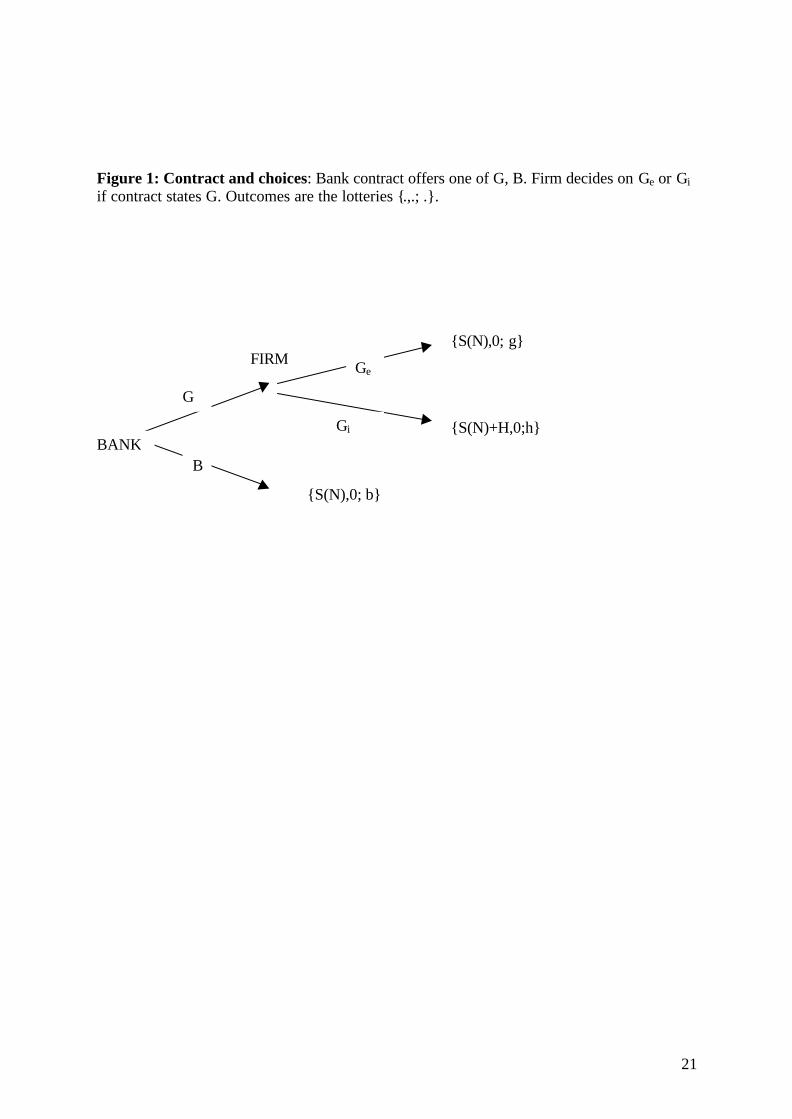
of this section. The investment choice is more clearly shown in Figure 1. Reading across

from the left-hand node, the bank offers a G or a B contract; the firm decides whether to

adopt Ge or Gi if it has accepted G, and then the outcomes result. Since banks are

competitive, no one bank can limit the choice of contract, only the explicit moral hazard

danger can prevent G from being available to the candidate firm.

4

The good outcome X in the lottery {X,Y; p} depends on the number N of firms receiving

contracts since each such firm supplies one unit to the market and hence more firms means

more product supply and lower product price, whether or not that firm is successful (thus the

level of costs incurred determines "success"). The more units sent to the market (higher N),

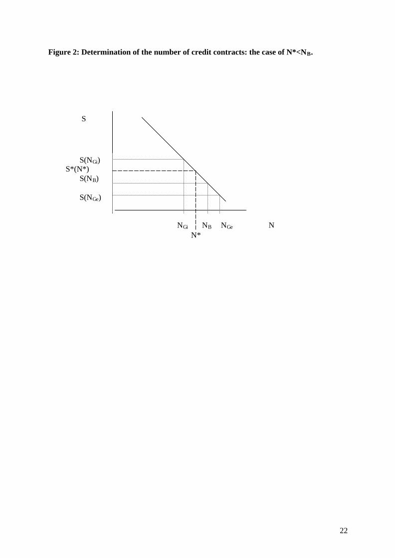
the lower the surplus S of successful firms. The schedule S(N) thus has a negative slope as

depicted in Figure 2. Firms that are not successful have production costs that exceed revenue

and hence these firms have a zero cash surplus. These unsuccessful firms cannot repay any of

their loan. In equilibrium all successful firms will repay the required D to the bank. We

define the surplus S(NGe) and the associated number of firms NGe as the surplus and number

of firms that would be a competitive equilibrium if no other technology than Ge were

available (and so no problem of technology choice existed). Entry would make expected

surplus equal finance and effort costs. Similarly for S(NGi), NGi, and S(NB), NB. Thus:

g S(NGe) = R + F (1)

h (S(NGi) + H) = R + F (2)

b S(NB) = R + F (3)

The better the technology, the more firms will be present in a single-technology competitive

equilibrium, and to ensure that the moral hazard problem is relevant when all three

technologies are available we will assume that

NGe > NB > NGi

Or equivalently:

S(NGe) < S(NB) < S(NGi)

Or equivalently in competitive equilibrium (using (1)-(3) above):

5

(R+F)/g < (R+F)/b < (R+F)/h –H (4)

This assumption, incorporated in Figure 2, simply states that it is most efficient to use the

firm’s discretion, efficiently applied, and least efficient to use the firm’s discretion,

inefficiently applied. (4) implies that g > b > h. The full information equilibrium would be

that NGe contracts would be issued and each firm would be required to use technology Ge and

the repayment for a successful firm would be R/g leaving the lending banks with zero

expected profit. To rule out this first-best outcome, the asymmetric information gives rise to

moral hazard for the firm if expected profit is higher if it uses Gi rather than Ge at NGe:

g (S(NGe) – R/g) – F < h(S(NGe) + H – R/g) – F (5)

The LHS of (5) is the expected net surplus for the firm choosing Ge. With probability g it

receives S(NGe) but pays the bank R/g. With probability 1-g, it fails and neither receives

surplus nor repays the bank. F is an additional effort cost which the firm incurs whether or

not it is successful. The RHS of (5) is the same expected outcome if Gi is chosen instead, but

the contract terms still require a repayment of R/g if the firm has funds. The inequality (5)

assumes that the firms have an incentive to play Gi rather than Ge. We assume that such

moral hazard exists ((5) holds). We can now consider two candidate equilibria.

Credit Rationing Equilibrium

In this equilibrium banks give discretion to the firms but influence firms’ behaviour by

rationing the number of contracts. For the firms to find it in their interest to choose Ge rather

than Gi we need a number of contracts N and a repayment D such that

6

g (S(N) – D) – F ≥ h(S(N) + H – D) – F (6)

and

gD = R from the assumption of competitive banks. Thus setting both sides of (6) equal we

have that

S*(N*) = R/g + hH/(g-h) (7)

is the lowest S* (arising from the highest number of contracts N* in Figure 2) such that the

firm will choose Ge rather than Gi. Intuitively, if further contracts were offered giving

discretion and requiring repayment of R/g, then firms would choose to seek higher profit via

the very risky and inefficient investment Gi. In fact, no bank would wish to offer a further G

contract additional to N* since this would render all G contracts loss-making to banks,

including the additional contract. A bank could offer a contract with repayment R/h (which

would break-even on average if firms chose Gi) but this would not be attractive to the firm if

there was no positive expected profit from deviating to Gi at the higher debt repayment:

h(S*(N*) + H) – R – F < 0. We will show below that this "stability condition" holds provided

that it is not profitable for B contracts to be offered and accepted in this equilibrium.

Credit Restriction Equilibrium

Here banks choose contracts with restrictions on the investment, thus the project is enforced

as B. Since there is a competitive banking system and an infinite number of potential firms,

7

the number of contracts and the repayment level are such that banks make zero expected

profits (D = R/b) and firms make zero expected profits (equ.(3) holds). It must not be

profitable to offer and accept G type contracts.

3. Analysis

We can state the following result.

Proposition 1: (a) The Credit Restriction equilibrium exists and is unique if S(NB) < S*(N*).

(b) The stability condition h(S*(N*) + H) – R – F < 0 holds if S(NB) ≥ S*(N*), and a Credit

Rationing equilibrium exists and is unique if S(NB) > S*(N*). (c) If S(NB) = S*(N*) then

both equilibria and any mix of the two kinds of contracts amounting to the same number of

contracts in total is also an equilibrium.

Proof

(a) The Credit Restriction equilibrium holds since Gi is loss-making at S(NB) That is:

h(S(NB) + H) – R – F < 0 since NB>NGi and using (2).

and Ge is not incentive compatible since S(NB) < S*(N*) for any contract:

g (S(NB) – R/g) – F < h(S(NB) + H – R/g) – F since NB>N* and using (7).

(b) The stability condition requires that h(S*(N*) + H) < F+R, so that a contract priced at

D = R/h could not be introduced, given that the firm would choose Gi. Now since

S*(N*) < S(NB) = (R+F)/b, the stability condition certainly holds if h((R+F)/b + H) <

F+R. But this is assumed in (4) – that S(NB) < S(NGi).

The Credit Rationing equilibrium holds since B is loss making with N*>NB contracts

8

already in existence (using (3) and N*>NB), Ge is incentive compatible (by definition

of N*) and Gi is loss-making as the stability condition holds.

(c) If S(NB) = S*(N*) then any combination of contracts G and B of total number NB=N*

satisfy incentive compatibility for the G contracts and zero profit for the B contract

((3) and (6) hold with equality), and the stability condition holds to ensure that further

contracts implying Gi (not Ge, since incentive compatibility would then fail) would

not be profitable with debt repayment R/h. Note that the zero profit for B contracts

means that no bank can profitably increase the number of B contracts it gives, even

though this would spoil the incentive structure for G contracts.

Figure 2 depicts the Credit Restriction equilibrium since S*(N*) > S(NB). It is interesting to

note that the contract regime can switch with changes in the parameters which reverse the

ordering of S*(N*)and S(NB). Moving from the case in Figure 2 to a Credit Rationing

equilibrium by shifting upwards S(NB) above S*(N*) has drastic effects on the industry. First,

the technology changes from the inefficient B to the efficient Ge. Second, expected profits of

firms change discontinuously from zero to positive amounts. To see the latter, write the

expected profit from a G contract with firms’ choice of Ge being incentive compatible as

π = gS*(N*) – (R + F) = g(S*(N*) – S(NGe)) > 0 (8)

using (1) and N*<NGe.

Parameter changes could switch the equilibrium from one of Credit Restrictions to one of

Credit Rationing. They are identified by considering when NB and N* will change places,

9

from the comparative statics effects on S(NB) – S*(N*), using (3) and (7):

S(NB) – S*(N*) = [ R (g-b)/g + F – bhH/(g-h) ] /b (9)

Thus we see immediately that the equilibrium could switch from Credit Restrictions to Credit

Rationing if there were the following changes:

i. Increase in g or decrease in b (this makes Ge even better than B)

ii. Decrease in h or H (this makes Gi less tempting for firms)

iii. Increase in R or F (this increases common costs and makes incentive compatibility less

costly to impose).

If such a change occurred with only a very small change in N then the only large impact on

welfare would be that the more efficient technology would imply strictly positive expected

profits for firms. Basically the new contracts would involve a more efficient technology but

the number of firms and hence supply would be limited to (about) the same levels as before.

Profits would be gained by firms but no other agents (banks, consumers) would gain.

Of course, movement the other way, such that the Credit Rationing equilibrium was replaced

by a Credit Restriction equilibrium would have both opposite causes and opposite effects.

Varying values of g for example could lead to cycles of equilibrium type. Clearly contracts

are placed for a period of time, during which the economic environment may change. Some

of the issues concerning regime change are taken up in the next section.

10

4. Extensions

In this section, we will consider some extensions and implications of the two equilibria that

we have discussed. The fact that a Credit Restriction equilibrium has been identified implies

that gains from improving the quality of control and reducing the loss from restricting

discretion can be found. We can use the concept of credit restrictions to apply to a number of

mechanisms for out-sourcing and auditing. Also, the market for credit can be avoided by

firms with their own finance, and this leads to possibilities for explaining the importance of

internal finance. Finally, we can use the regime switching argument to apply to recent

changes in the international business climate, both in terms of the growth and the decline of

managerial discretion.

Incentives for banks

The technology B may be bank-specific. A bank willing to research the industry can exert

better control and set better rules than other banks. We will consider a departure from our

assumption of competitive identical banks in order to consider the reward for a quality bank

which can offer a better technology B than other banks. If the current equilibrium is a Credit

Restriction equilibrium then the quality bank can propose a contract that offers slight positive

expected profits to firms and hence supply finance to all firms. Suppose the contract offered

to the firm is for a technology {S(N),0; q} and the repayment required is (virtually) q S(N) –

F, for N ≥ NB, so that firms' profits are virtually zero. Note that the quality bank cannot

reduce N below NB since then other banks will provide contracts to make up the total number

to NB. The quality bank would make an expected monopoly profit of at least (q S(NB) – F –

R) NB = (q-b)(F + R)NB/b (using (3)). If (q S(N) – F – R) N is increasing in N at NB then the

11

quality bank could make a still higher expected profit by offering more contracts despite the

reduction in repayment per successful contract (despite the lower S(N)).

If the initial equilibrium was a Credit Rationing equilibrium, then the quality bank may be

able to impose a regime switch by its better B contract. It would have to keep the number of

contracts at least as high as before (in this case N ≥ N*) since G contracts from other banks

would otherwise make up the difference to N*. However, the repayment would not have to

allow the same expected profit as before, since the choice of any N > N* would render the Ge

technology not incentive compatible if offered to any firm by any bank. Thus the monopoly

profit would be the same as in the first case since the only competition is from contracts of

type B. Hence the Credit Restriction contracts would replace the Credit Rationing

equilibrium, since N* contracts could be offered by the quality bank if (q S(N*) – F – R) N*

> 0. Note that it is possible for this to occur even though N* contracts for G could offer

positive profits for the firms. The point is that the quality bank can unilaterally spoil the

ration by adding another contract of type B and hence raising N above N*. Equilibria can

exist with no G contracts if (q S(N) – F – R) N is increasing in N at N = N*. If further banks

obtained the same “quality” then competition would lead to a new Credit Restrictions

equilibrium with q replacing b.

Type of restrictions

The formulation of restrictions on how the credit can be used can vary from a continuous

monitoring process (such as membership of boards of directors) which would impose

particular views and concerns on the firm's decisions, to policies such as whether and how to

source connected work from outside the firm. One example might be the requirement to

12

spend the credit on particular products from firms which are known to be reliable, rather than

on the "best deal" which might involve high risks. This might lead to requirements to deal

with suppliers offering quality marks, or suppliers in particular countries less prone to

corruption. A further restriction might require that supply is not organized “in-house”. Thus

the requirement to out-source key inputs might be a safeguard against risky internal

production plans. A feature of all kinds of restriction is that the credit would be used in a way

that could be monitored by the bank or by the firm's auditors.

The use of restrictions to deny the firm the temptation to risk the bank's investment will

inevitably reduce the profit possibilities as well as the loss possibilities. The quality of the

restrictions in minimising the former for any given gain in risks of loss are obviously key.

The development of venture capitalists2 might be thought to be an institutional response to

the need for providing both monitoring and restrictions on expenditure and experience and

judgement in decision making.

Our model of credit rationing follows the (Blanchard and Fischer, 1989, p479) type 2 format

since credit is rationed among firms, with some firms going without. An alternative type 1

format would supply all firms with credit but at a lower level than they desire. This may be

thought to be another form of credit restriction: a firm may only borrow up to a binding

constraint. In the absence of other finance, the firm must then choose only smaller capital

projects, and this may remove or reduce the moral hazard issue. In this case, the credit

restriction versus credit rationing assessment becomes a type 1 or 2 credit rationing

assessment.3

2 See for example Hellman and Puri (2000).3 A key motivation behind the type 1 credit rationing model is to make firms increase their own financialcommitment to the project and hence be less prone to moral hazard and more likely to repay. Obviously our

13

Firms with internal finance

There may be firms in the industry with their own finance, and that therefore do not need to

obtain loans from banks. Suppose that this is the case but that the number of such firms is less

than NGi . The analysis is then largely unaltered. Clearly these firms will choose Ge (from

(1)). In either a Credit Rationing equilibrium or a Credit Restriction equilibrium these firms

will make positive expected profit (the same as other firms in the former, and (g-b)(F + R)/b

in the latter). In terms of Figure 2 and considering N as the number of bank contracts, the

S(N) schedule is shifted to the left, but not so far as to eliminate all space for firms needing

bank finance. An interesting aspect is that the situation might arise where the firms with their

own finance adopt Ge while firms which need outside finance adopt B because Ge would not

be incentive compatible for them and so finance cannot be obtained except under restrictive

contracts. This would imply that there would be two technologies active in an industry, with

rich firms gaining from poor firms' credit limitations.4

Application to changing circumstances.

We have discussed in section 3 how an equilibrium can switch between one of credit

rationing and one of credit restrictions. If the equilibrium can be disturbed by a change in the

parameters involved then inertia in contracts means that the system is liable to a specific

chain of events. For example, suppose g decreases because profits from (say) high technology

or telecoms projects were found to be less likely. Continuing Ge contracts, which could not be

model does not explicitly include such the option of an internal finance contribution as part of the financialcontract, but the implication is clear.

14

changed in the short run, would become incentive incompatible (see (5)) and firms or their

managers would choose Gi instead. For example, they may continue to develop projects that

should have been curtailed, on the basis that the market just might improve. Many of these

firms will fail because of the high risk of this strategy. The outcome will eventually be a new

equilibrium regime with the adoption of the B technology. A period of conservative and

relatively less entrepreneurial investment will then ensue. Again, the economic environment

might change and the view that desirable Ge contracts can be implemented, using the firm's

own management expertise and a withdrawal from creditor control, would shift the

equilibrium to a Credit Rationing equilibrium. However, if the number of credit contracts

become too large given the true opportunities then N>N* will lead to moral hazards. Banks

or other creditors will have less faith in leaving discretion to firms in volatile times when Ge

is likely to change. In terms of recent experience of firm failures5 and issues to do with the

non-disclosure of changing profitability, the prediction of this line of argument is for a more

intrusive creditor boardroom presence and less discretion for firms until governance, auditing

and stability respond.

Endogenous Hazards

It is probably unnecessary to confirm these conjectures within a formal model, but one

particular driving force of cyclical behaviour might be of interest. Consider that the moral

hazard temptation is to gain H in the G contract. Suppose that the level of H is subject to

dynamic effects. In particular H in period t is related to previous period’s H, plus a value

dependent on the regime (Credit Restriction or Rationing) plus a noise term:

4 This result is explored in a further paper, Ireland (2002). In particular, continuing firms are assumed to havethe advantage of internal finance, while entrants have to find external finance. The roles of venture capitalists as"high quality" banks giving relatively good restricted B contracts, and of shared equity finance, are considered.

15

Ht = λHt-1 + St-1 + θt-1 (10)

where 0<λ<1, St = s+a, if the regime in period t is Credit Rationing, St = s-a if the regime is

Credit Restrictions, and a>0. θt has a zero mean. Since the noise term is lagged, there is no

uncertainty when fixing the t-period’s contract. 6 If a=0 then the model is just a series of

shocks to the level of H, sometimes creating the need to change to a Credit Restrictions

equilibrium. If a≠0 then changes of regime are possible even in the absence of shocks.

The different values of S are meant to reflect the more adventurous seeking of profits that

takes place when firms have discretion: firms’ moral hazard temptation H grows to a level of

(s+a)/(1-λ) in the absence of stochastic effects. In times of credit restrictions, H adjusts to the

lower level (s-a)/(1-λ). Thus even in the absence of stochastic effects via θt, Ht will grow

higher in times of credit rationing, and might trigger a shift to credit restrictions. The question

is merely if the particular H value (denoted Hs) that makes N* = NB in (9) satisfies

(s-a)/(1-λ)<Hs<(s+a)/(1-λ) (11)

The reverse regime switch would also occur, since the equilibrium path for H would have

become downward sloping in the Credit Restrictions equilibrium. The additional presence of

stochastic shocks means that such cycles will be of variable and unpredictable period. It also

means that there is always some chance of triggering a change in regime within a finite time.

5 In 2001 95 "big, publicly owned companies" filed under Chapter 11 protection in the USA. This total is likelyto be exceeded in 2002. (Economist, Sept 7th 2002, p71)6 A contemporary shock would require some additional analysis of contract setting since the H parameter in Giwould not be known with certainty. The lag in the St variable is meant to indicate a time to learn aboutcandidates for the Gi project.

16

The stochastic and non-linear features of (10) mean that many kinds of behaviour could be

generated. However, the key characteristic is the tendency to cycle from one regime to the

other. This may be observed in the non-stochastic case in the long run as a limit cycle, with

oscillations either side of Hs from one period to the next. A requirement for this is that Hs

satisfies

s/(1-λ) – a/(1+λ) <Hs< s/(1-λ) + a/(1+λ) (12)

(rather more restrictive than (11) above). If the regime switches each period then assume that

at some t:

Ht+1 = λ Ht + s + a (13)

Ht = λ Ht-1 + s – a (14)

so that

Ht+1 = λ2 Ht-1 + λ(s – a) + s + a (13’)

and

Ht = λ2 Ht-2 + λ(s + a) + s – a (14’)

Consider (13’) and (14’) as separate equations (one for even and one for odd time periods, for

example). In the long run the homogeneous solutions of both equations tend to zero and the

particular solutions are

17

Hp = [λ(s – a) + s + a]/(1-λ2) = s/(1-λ) + a/(1+λ)

for alternate periods t+1, t-1, t-3, t-5,… (13’’)

Hp = [λ(s + a) + s – a] /(1-λ2) = s/(1-λ) - a/(1+λ)

for alternate periods t, t-2,t-4,t-6,… (14’’)

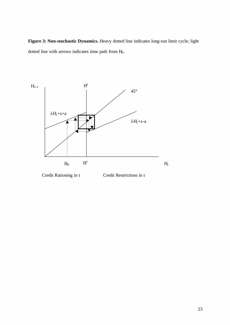
Provided Hs satisfies (12), the assumed regime changes are confirmed. Figure 3 shows the

dynamic path of this case: after possibly chaotic initial adjustments the cobweb pattern

converges to a limit cycle (shown by the heavy-dotted-line rectangle). (11) ensures that, at Hs,

λH + s + a > H and so lies above the 45° line, and λH + s – a < H and so lies below the 45°

line. Small variations in Hs do not affect the cycle. However if Hs increased so much that it

was to the right of the limit cycle (Hs > Hp in (13’’)), then more than one period would be

spent in the Credit Rationing regime before switching to the Credit Restrictions regime. This

represents the case where H has to be very high before it is sufficiently problematic to trigger

the switch. The restriction (12) rules out the complications of these kinds of asymmetric

cycles where more periods are spent in one regime than in the other.

The notion that moral hazard opportunities would expand as periods of firms’ discretion

become larger may be of wider interest. One can think of a gradual reduction of banks’

ability to monitor firms as they rely increasingly on credit rationing and firms own decision

making. Similarly, the imposition of a Credit Rationing equilibrium may take time to have

complete effect as banks have to learn the right ways of writing restrictions into contracts and

monitoring firms’ compliance. At the end of the day, however, banks will come to accept that

their control is against the interests of efficiency when temptations of firms are sufficiently

small. Then a switch to relying on firms having profit incentives to avoid inefficient projects

will occur, only to be gradually eroded as firms’ discover additional temptations. The regime

18

cycle is of course mirrored by a cycle of relative success of projects, and also of the number

of projects financed. Changing H does not change NB, only N*.

A number of formulations of firms’ balance sheet effects on cyclical behaviour via financial

markets include Greenwald and Stiglitz (1993). They are concerned with the ability of profits

to create better hedges to avoid bankruptcies and hence higher investment. In our argument

here, we are focussing on the (possibly complementary) propensity of the financial system to

change mechanisms and hence create cycles of activity. 7

5. Conclusions

This paper has used a very simple model of regime changes which can only be indicative of

the kind of shift that may occur. In particular, the characterisation of contract outcome is very

simple, and of course there may be many differences among markets and industries at any

one time as well as changes in regime over time. Nevertheless, the analysis brings together

two rather different literatures and sees their contributions as complementary.

The major argument we have made is that the equilibrium system of contracting loans may

change radically due to changes in opportunities and perceptions. A system which is based on

delegation and discretion may be rejected in favour of monitoring and lender control when

experience suggests an increase in moral hazard. Such changes in equilibrium may take some

time to be implemented due to the lags in contract renewal. One factor in recent experience is

that large and apparently diversified firms which were perhaps thought to be immune to

7 See Arnold (2002) for a recent survey of business cycle models.

19

moral hazard issues have been found to be as affected as smaller firms. Thus the importance

of the equilibrium systems discussed here has increased with their relevance.

A number of the factors considered may deserve further analysis. The specific nature of the

loan contracts and their description in terms of success and failure are not likely to be

fundamental to the broad nature of the analysis. However, other types of finance including

equity holdings and internal finance, together with the different nature of firms’ collateral

within the comparative equilibria, are topics which could be investigated within the

framework presented here. In the presence of nominal rigidities the varying number of

projects financed can clearly cause changes in employment, but a more general equilibrium

approach would be required to investigate that issue.

20

References

Arnold, Lutz G. (2002) Business Cycle Theory. Oxford: Oxford University Press.

Blanchard, Oliver J. and Fischer, S (1989) Lectures on Macroeconomics. Cambridge: MITPress.

Clemenz, Gerhard (1986) Credit Markets with Asymmetric Information. Springer-Verlag,Berlin.

De Meza, David, and Webb, David (1987) Too much investment: a problem of asymmetricinformation. Quarterly Journal of Economics, 102: 281-292.

De Meza, David, and Webb, David (2000) Does credit rationing imply insufficient lending?Journal of Public Economics, 78: 215-234.

The Economist (2002) The firms that can't stop falling. Sept 7th : 71-2.

Greenwald, B and Joseph E. Stiglitz (1993) Financial market imperfections and businesscycles. Quarterly Journal of Economics, 108: 77-114.

Grossman, Sanford J., and Hart, Oliver (1988) One share / one vote and the market forcorporate control. Journal of Financial Economics, 20: 175-202.

Hart, Oliver (2001) Financial contracting. Journal of Economic Literature 39 (4): 1079-1100.

Hart, Oliver, and Moore, John (1998) Default and renegotiation: a dynamic model of debt.Quarterly Journal of Economics, 113: 1-41.

Hellman, Thomas and Puri, Manju (2000) Venture capital and the professionalization of start-up firms: empirical evidence. Stanford University Graduate school of Business, researchpaper 1661.

Ireland, Norman (2002) Technology Choice Bias and Limited Liability. mimeo, University ofWarwick

Kaplan, Steven and Stromberg, Per (2000) Financial contracting meets the real world: anempirical study of venture capital contracts. working paper, University of Chicago, GraduateSchool of Business.

Stiglitz, Joseph E. (1985) Credit markets and the control of capital. Journal of Money, Creditand Banking, 17: 133-152.

Stiglitz, Joseph E. and Weiss, Andrew (1981) Credit rationing in markets with imperfectinformation. American Economic Review, 71: 393-410.

21

Figure 1: Contract and choices: Bank contract offers one of G, B. Firm decides on Ge or Giif contract states G. Outcomes are the lotteries {.,.; .}.

FIRM

BANK

G

B

Ge

Gi

{S(N),0; b}

{S(N),0; g}

{S(N)+H,0;h}

22

Figure 2: Determination of the number of credit contracts: the case of N*<NB.

S

NGi NB NGe N N*

S(NGi)S*(N*) S(NB)

S(NGe)

23

Figure 3: Non-stochastic Dynamics. Heavy dotted line indicates long-run limit cycle; light

dotted line with arrows indicates time path from H0.

λHt+s-a

λHt+s+a

45°Hs

HtH0

Ht+1

Credit Rationing in t Credit Restrictions in t

Hs