Raven Pro 1.4 User’s Manual Revision 11 10 December 2010 This manual can be printed or used online. To access all online fea- tures, we recommend viewing with the latest version of Adobe [Acrobat] Reader, available free at http://www.acrobat.com. For online viewing, use the bookmarks in the navigation pane on the left to navigate to sec- tions within the manual. Cross references in the text and index entries are hypertext links: click the link to view the referenced section or page.
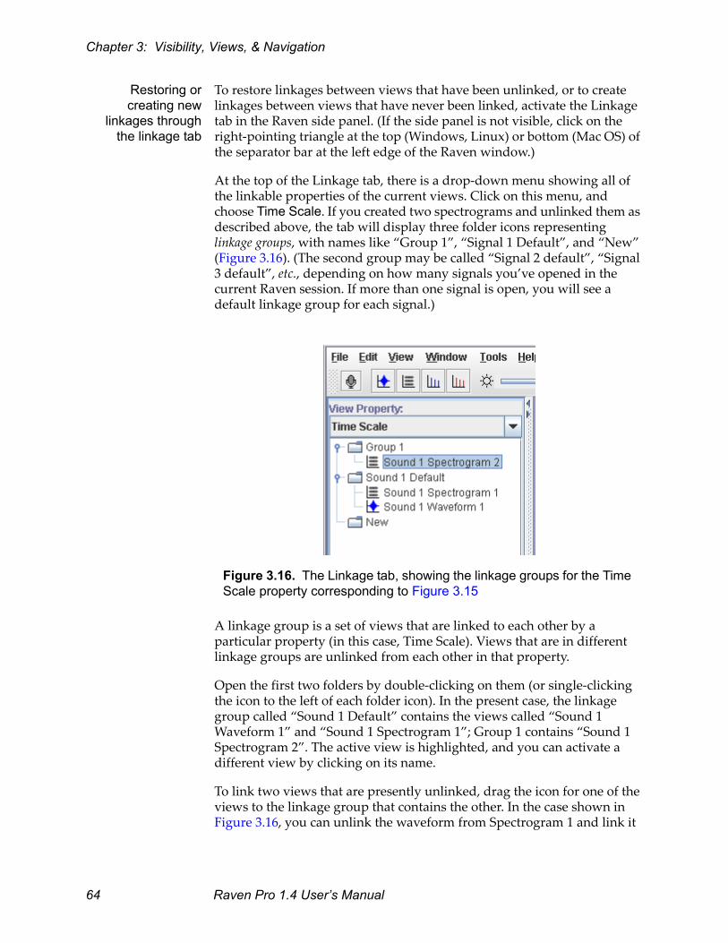
Transcript
Raven Pro 1.4 User’s ManualRevision 11
10 December 2010
This manual can be printed or used online. To access all online fea-tures, we recommend viewing with the latest version of Adobe [Acrobat] Reader, available free at http://www.acrobat.com. For online viewing, use the bookmarks in the navigation pane on the left to navigate to sec-tions within the manual. Cross references in the text and index entries are hypertext links: click the link to view the referenced section or page.
The Raven software includes code licensed from RSA Security, Inc. Some portions licensed from IBM are available at http://oss.software.ibm.com/icu4j/.
TrademarksMicrosoft and Windows are registered trademarks of Microsoft Corporation in the United States and/or other countries. Mac and Mac OS are registered trademarks of Apple Computer, Inc. Linux is a registered trademark of Linus Torvalds. PostScript is a registered trademark of Adobe Systems, Inc. Java is a registered trademark of Sun Microsystems, Inc. Other brands are trademarks of their respective holders and should be noted as such.
Mention of specific software or hardware products in this manual is for informational purposes only and does not imply endorsement or recommendation of any product. Cornell University and the Cornell Lab of Ornithology make no claims regarding the performance of these products.
CreditsRaven was developed with partial support from the US National Science Foundation (grant DBI-9876714, Principal Investigators: Christopher W. Clark and Kurt M. Fristrup), with additional support from the Cornell Lab of Ornithology.
Raven software was written by Harold Mills, Tim Krein, Dean Hawthorne, Scott Maher, Andrew Jackson, Aisha Thorn, Dounan Hu, Laura Strickman, Christina Ahrens, Jason Rohrer, and Jason Adaska.
The Raven User’s Manual was written by Russell A. Charif, Amanda M. Waack, and Laura M. Strickman with contributions by Tim Krein, Dean Hawthorne, Ann Warde, Dimitri Ponirakis, Wendy Alberg, and Sarah Smith.
Raven artwork by Diane Tessaglia-Hymes.
The Raven development project is led by Tim Krein and is under the general direction of Christopher W. Clark.
CitationWhen citing use of Raven in scientific publications, please refer to the software by referring to the Raven website: www.birds.cornell.edu/raven
When citing use of this manual, please refer to it as follows:
Charif, RA, AM Waack, and LM Strickman. 2010. Raven Pro 1.4 User’s Manual. Cornell Lab of Ornithology, Ithaca, NY.
For more information about Raven, visit the Raven website: www.birds.cornell.edu/raven
Bioacoustics Research ProgramCornell Lab of Ornithology159 Sapsucker Woods Rd.Ithaca, NY 14850USA
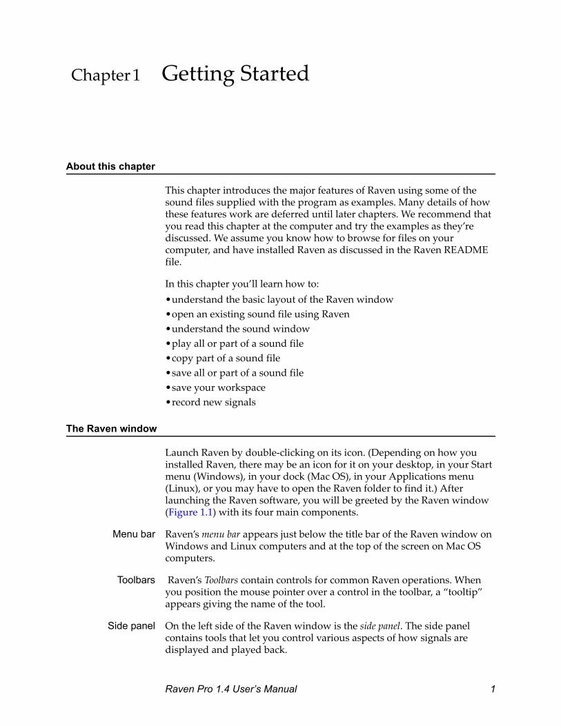
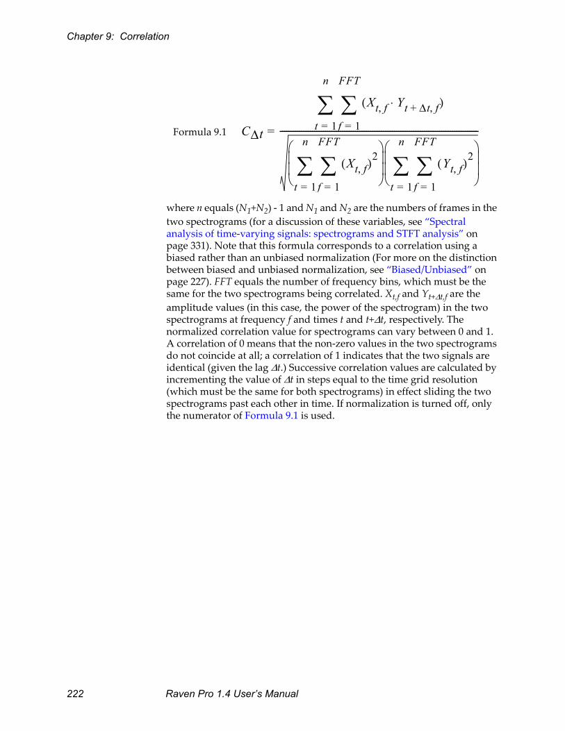
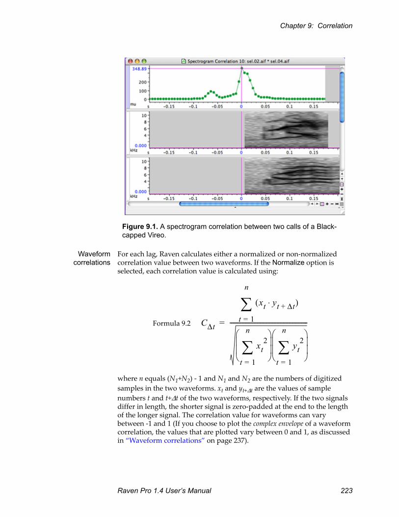
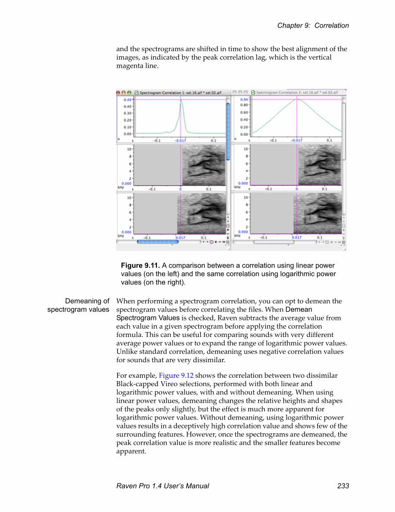
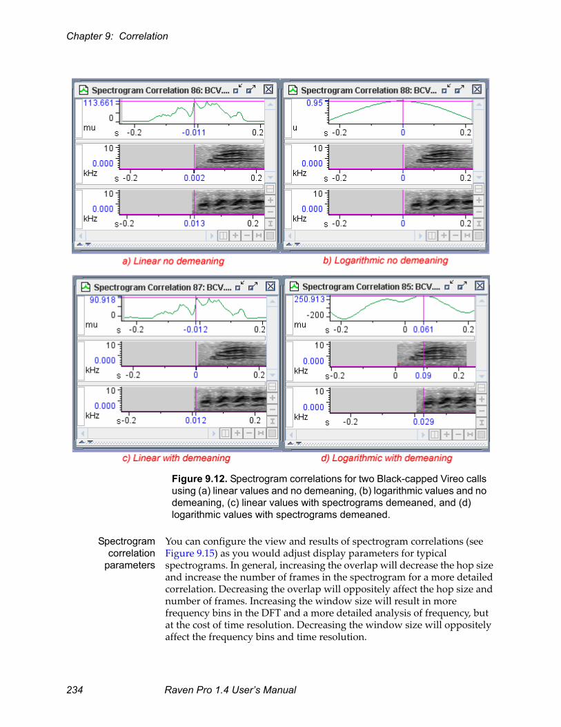
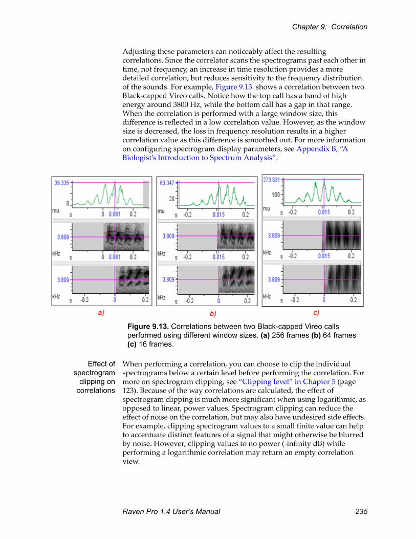
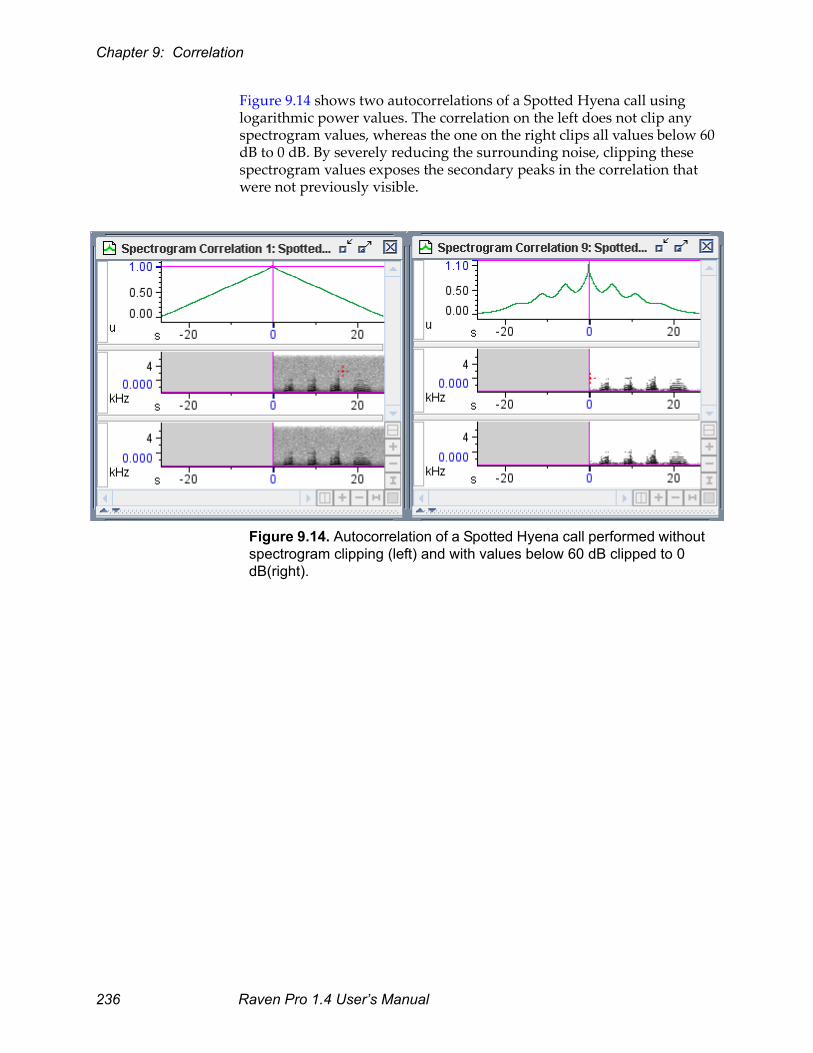
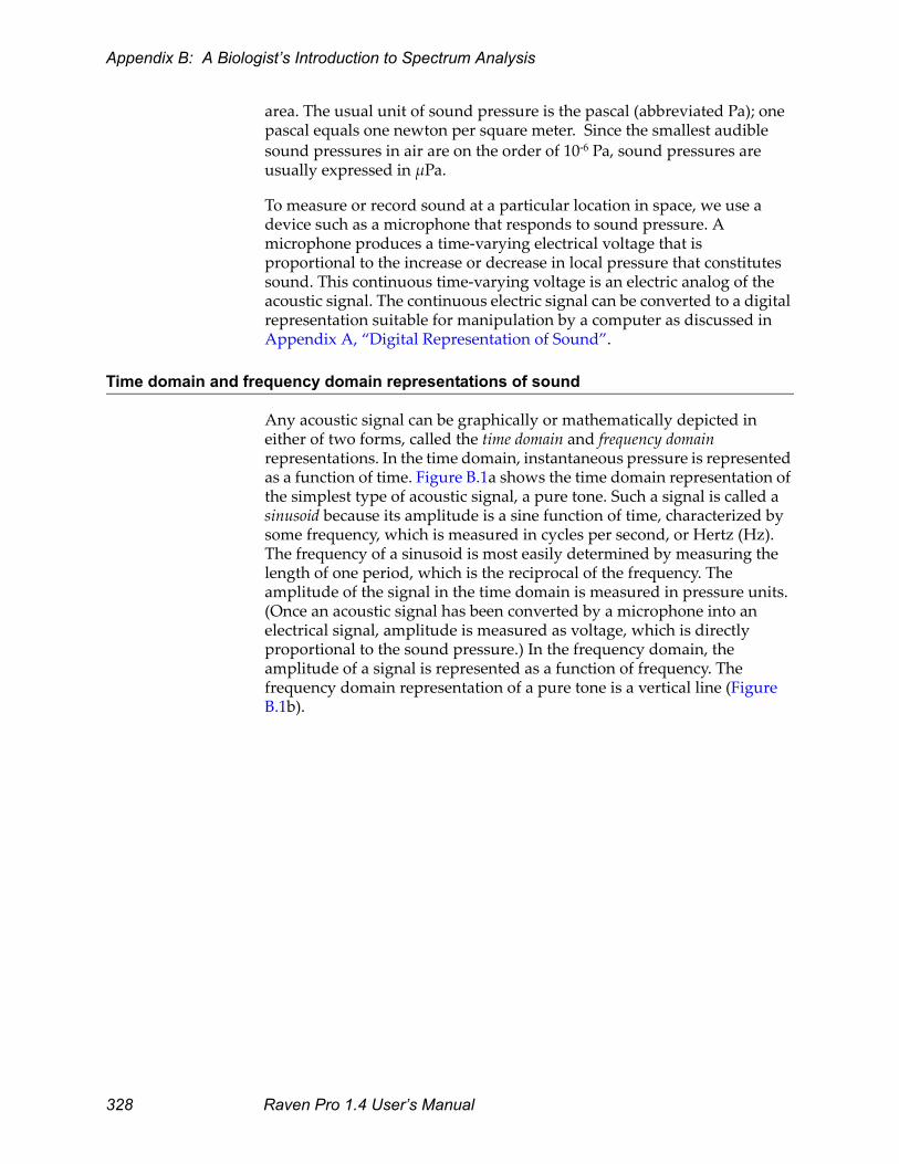
This chapter introduces the major features of Raven using some of the sound files supplied with the program as examples. Many details of how these features work are deferred until later chapters. We recommend that you read this chapter at the computer and try the examples as they’re discussed. We assume you know how to browse for files on your computer, and have installed Raven as discussed in the Raven README file.
In this chapter you’ll learn how to:•understand the basic layout of the Raven window•open an existing sound file using Raven•understand the sound window•play all or part of a sound file•copy part of a sound file•save all or part of a sound file•save your workspace•record new signals
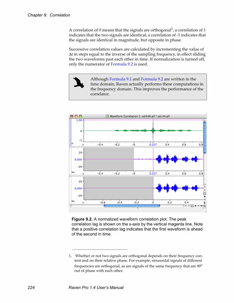
The Raven window
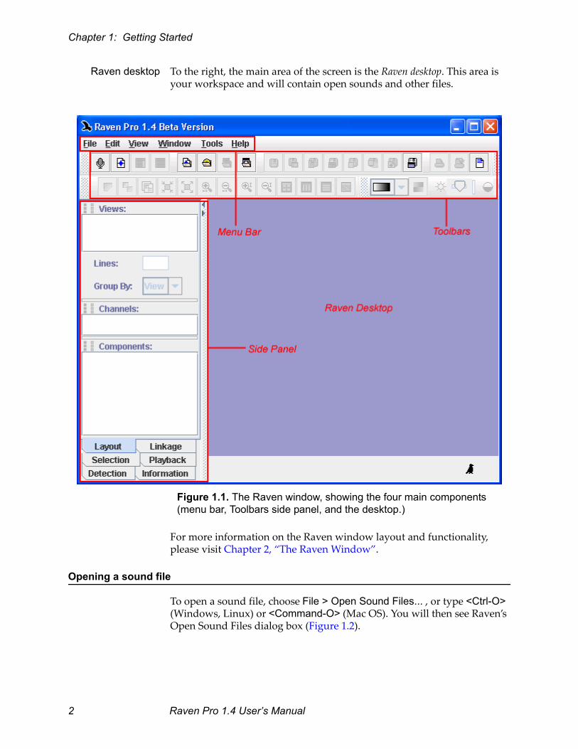
Launch Raven by double-clicking on its icon. (Depending on how you installed Raven, there may be an icon for it on your desktop, in your Start menu (Windows), in your dock (Mac OS), in your Applications menu (Linux), or you may have to open the Raven folder to find it.) After launching the Raven software, you will be greeted by the Raven window (Figure 1.1) with its four main components.
Menu bar Raven’s menu bar appears just below the title bar of the Raven window on Windows and Linux computers and at the top of the screen on Mac OS computers.
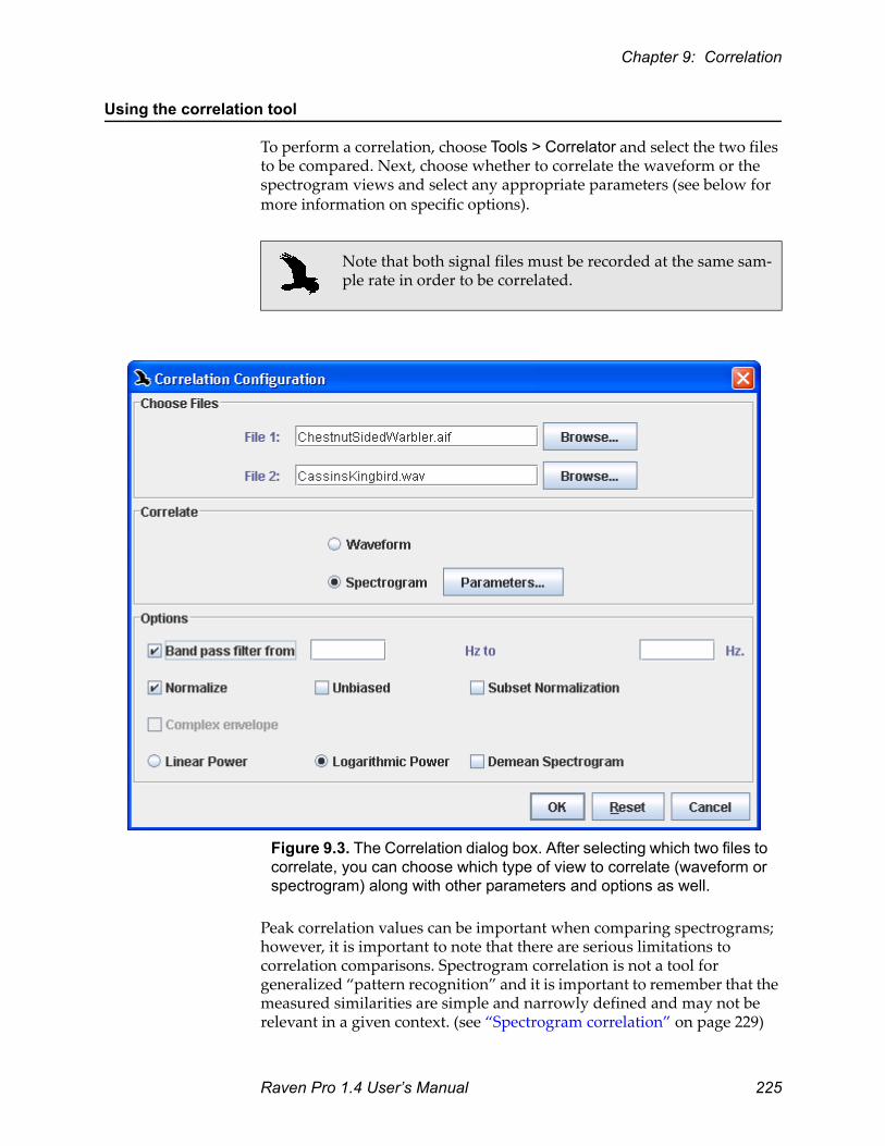
Toolbars Raven’s Toolbars contain controls for common Raven operations. When you position the mouse pointer over a control in the toolbar, a “tooltip” appears giving the name of the tool.
Side panel On the left side of the Raven window is the side panel. The side panel contains tools that let you control various aspects of how signals are displayed and played back.
Raven Pro 1.4 User’s Manual 1
Chapter 1: Getting Started
Raven desktop To the right, the main area of the screen is the Raven desktop. This area is your workspace and will contain open sounds and other files.
Figure 1.1 The Raven window
Figure 1.1. The Raven window, showing the four main components (menu bar, Toolbars side panel, and the desktop.)
For more information on the Raven window layout and functionality, please visit Chapter 2, “The Raven Window”.
Opening a sound file
To open a sound file, choose File > Open Sound Files... , or type <Ctrl-O> (Windows, Linux) or <Command-O> (Mac OS). You will then see Raven’s Open Sound Files dialog box (Figure 1.2).
2 Raven Pro 1.4 User’s Manual
Chapter 1: Getting Started
Figure 1.2 Open Sound Files dialog
Figure 1.2. Open Sound Files dialog box on a Windows computer (top) and a Mac OS computer (bottom).
The Open Sound Files dialog box displays a scrolling list of the files and directories in the current directory. The name of the current directory is given at the top of the dialog box. If the current directory is not “Examples”, find the Examples directory now in the Raven program directory. (To move up in the file system hierarchy, click on the name of
Raven Pro 1.4 User’s Manual 3
Chapter 1: Getting Started
the current directory and select another directory from the pull-down menu that appears. To move down the hierarchy, double-click on the name of a directory in the scrolling list of files and directories within the current directory.)
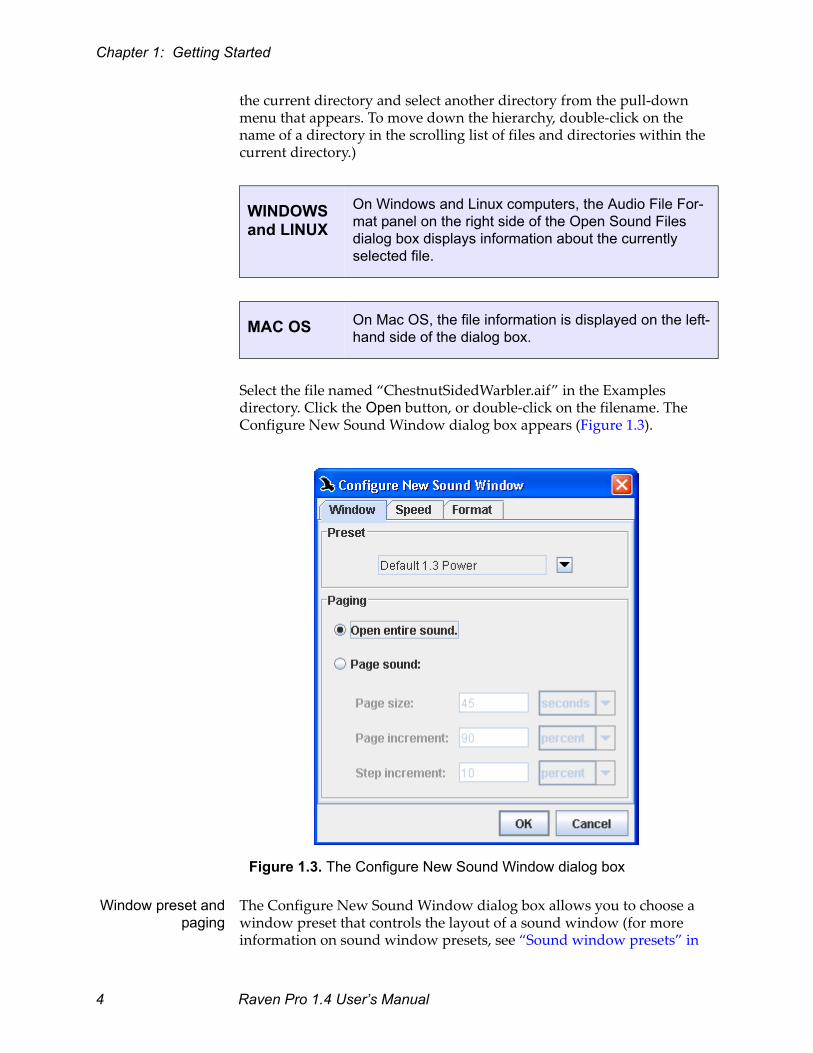
Select the file named “ChestnutSidedWarbler.aif” in the Examples directory. Click the Open button, or double-click on the filename. The Configure New Sound Window dialog box appears (Figure 1.3).
Figure 1.3. Configure New Sound Window dialog
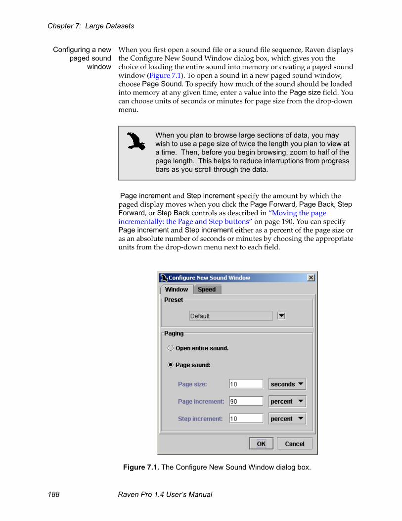
Figure 1.3. The Configure New Sound Window dialog box
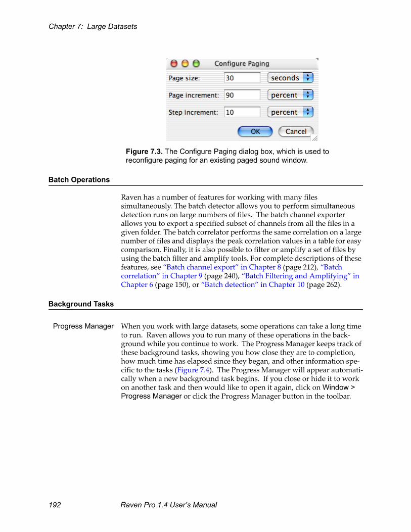
Window preset andpaging
The Configure New Sound Window dialog box allows you to choose a window preset that controls the layout of a sound window (for more information on sound window presets, see “Sound window presets” in
WINDOWS and LINUX
On Windows and Linux computers, the Audio File For-mat panel on the right side of the Open Sound Files dialog box displays information about the currently selected file.
MAC OS On Mac OS, the file information is displayed on the left-hand side of the dialog box.
4 Raven Pro 1.4 User’s Manual
Chapter 1: Getting Started
Chapter 11 (page 303)), and to control how much of the sound is loaded into Raven’s working memory at one time (see “About Raven memory allocation” in Chapter 11 (page 310) for more information on how Raven uses memory.)
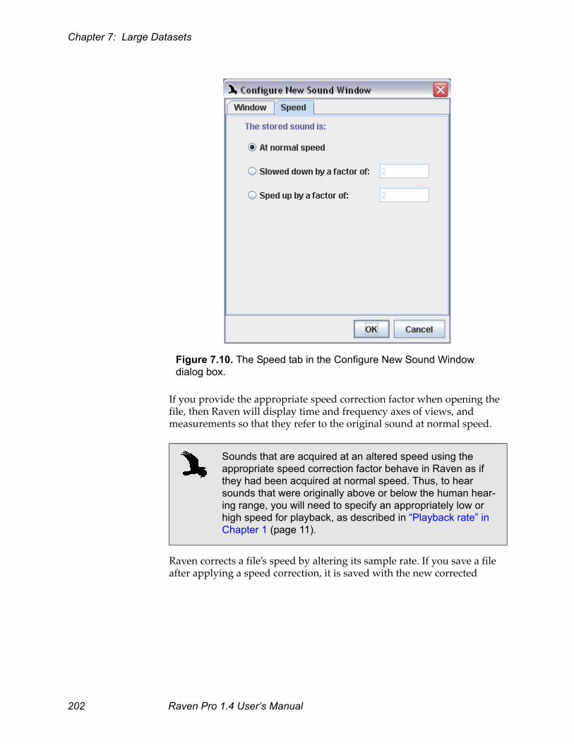
Speed correction The Speed tab of the dialog box gives you options to correct the recorded speed of a stored sound. For more information on this, see “Correcting speed when opening file” in Chapter 7 (page 201).
For now, click OK at the bottom of the dialog box to accept the default settings. A sound window appears on the Raven desktop (Figure 1.4).
File format The Format tab of the dialog box lists the formatting information associated with the chosen file. This information cannot be configured from this dialog, but may serve as a useful reference when choosing other settings.
Figure 1.4 Sound window
Figure 1.4. A sound window shown on the Raven desktop.
Raven Pro 1.4 User’s Manual 5
Chapter 1: Getting Started
The title bar of the sound window shows a sequential number (starting at 1) that Raven assigns to each sound you open, and the name of the file.
Opening sounds indifferent file formats
Raven also enables you to open sound files in .mp3 (with the exception of variable bitrate mp3 files), .mp4, .aifc, and QuickTime movie soundtrack (.mov) formats. In Raven Pro 1.4 build 33 and later, Raven opens these files without any additional setup. In versions of Raven earlier than build 33, in order to access files in these formats you must have QuickTime (QT) for Java installed on your computer. Raven can also open sound files in the .flac format, which does not require the installation of QuickTime. Raven does not include the ability to save sound files in these additional formats.
When Raven is running, you can open any WAVE or AIFF sound file by dragging its icon from an Explorer (Windows) or Finder (Mac OS) window or from the desktop and “dropping” the icon anywhere in the Raven desktop. If you hold down the Ctrl key (Command key on a Mac) while dropping the file, Raven will skip the Configuration dialog and open the sound with the current settings.
To open a recently used sound file, choose File > Open Recent Sound Files> fileName. By default, Raven displays the four most recent files. To open a file from a folder that you recently used within Raven, choose File > Open Recent Folder > folderName.
WINDOWS You can check whether QT for Java is installed by look-ing at the Download QuickTime Installer item on the Help menu. If QT for Java is already present, the menu item will be disabled. If the menu item is enabled, click on it and follow the instructions that appear in your web browser to install QT for Java.
MAC OS QT for Java is already installed on Mac OS computers. Mac OS users can also open CD audio tracks with Raven. Audio CD tracks will be displayed in the /Vol-umes folder as AIFC files that can be accessed from Raven’s Open Files dialog.
6 Raven Pro 1.4 User’s Manual
Chapter 1: Getting Started
Opening multi-channel files
Raven can open files that contain any number of channels. For informa-tion about how to open multi-channel files, see “Opening a multi-channel file” in Chapter 8 (page 205).
Opening files fromCanary
Raven Pro can open sound files saved in the Canary file format. Under Mac OS X, Raven Pro can open these files directly. In order to open Canary files in Raven Fro on a computer running Windows, you must first convert the files to MacBinary format on a Mac OS computer, then copy the files to the Windows machine. You can convert Canary files to MacBinary by using a free conversion program available at:
Note that while Raven Pro can open sound files saved by Canary in the Canary file format and in the AIFF file format, Raven Pro cannot open files saved by Canary in the MATLAB, SoundEdit, Text, or Binary formats.
Understanding the Sound Window
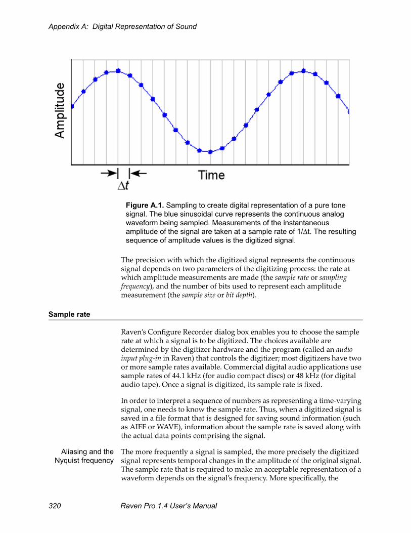
By default, when you first open a sound file, Raven shows you a sound window that contains two views of the sound (see Figure 1.5). The waveform (upper) view displays an oscillogram, or graph of the sound showing amplitude versus time. The spectrogram (lower) view represents time on the horizontal axis, frequency on the vertical axis, and relative power at each time and frequency as a color (by default grayscale) value. Spectrogram views are discussed further in “Spectrogram views” in Chapter 5 (page 129).
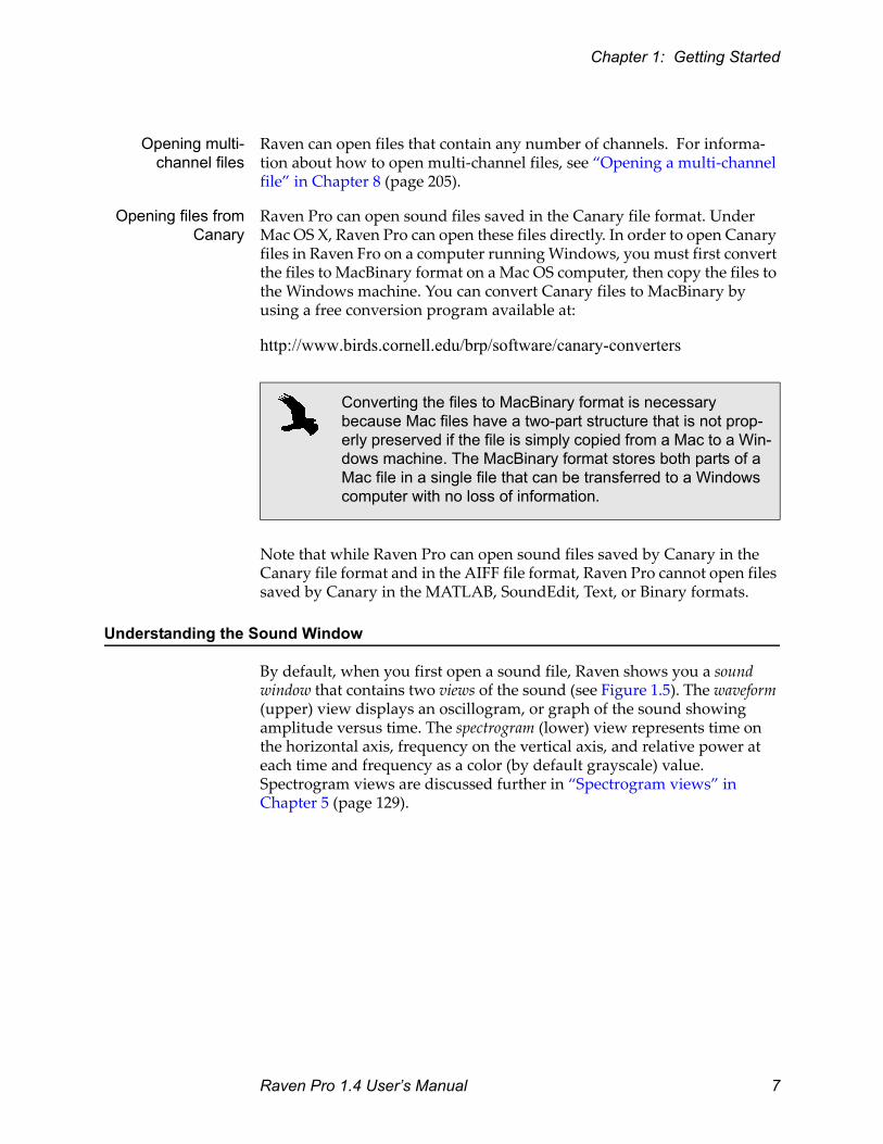
Converting the files to MacBinary format is necessary because Mac files have a two-part structure that is not prop-erly preserved if the file is simply copied from a Mac to a Win-dows machine. The MacBinary format stores both parts of a Mac file in a single file that can be transferred to a Windows computer with no loss of information.
Raven Pro 1.4 User’s Manual 7
Chapter 1: Getting Started
Figure 1.5 Sound window
Figure 1.5. A sound window showing a waveform view (top) and a spectrogram view (bottom).
In addition to waveforms and spectrograms, Raven can also display spectrogram slice views of a signal, and selection spectrum views, which show the average spectrum of a selected portion of a signal. Spectrogram slice views and selection spectrum views are discussed in “View Types” in Chapter 3 (page 56). Chapter 3, “Sound Windows: Visibility, Views, Linkage, & Navigation” also explains how to configure Raven to display combinations of views other than the default waveform and spectrogram when a signal is first opened.
Playing a sound
The sound playback controls can be found in the right-hand end of the play toolbar (Figure 1.6). Make sure the ChestnutSidedWarbler.aif sound window is open, as directed in “Opening a sound file” on page 2. To play the sound, click the Play button, or press <Ctrl-Shift-P> (Windows, Linux) or <Command-Shift-P> (Mac OS).
Figure 1.6
Figure 1.6. The playback controls in the play toolbar.
8 Raven Pro 1.4 User’s Manual
Chapter 1: Getting Started
As the sound plays, a vertical green line, the playback cursor, moves across the waveform from left to right to show you what part of the signal you are hearing. To stop playing at any time, click the Stop button. When the selection finishes playing, or when you click Stop, the playback cursor disappears.
Making a selection To choose a portion of the signal, click and drag your mouse from one point in the sound to another a point, in either the waveform or spectrogram view. Raven will mark your selection with a colored rectangle. For more about making selections, see Chapter 6, “Selections: Measurements, Annotations, & Editing”.
Playing a selectedpart of a signal
Once you’ve made a selection, you can choose to play only that portion of the sound by clicking the Play button. Clicking the Play button with an active selection will only play the visible portion of the selection. If the active selection is not currently visible, the Play button will play the entire visible portion of a sound. To play the entire visible portion of a sound with a selection active, use the Play Visible button.
Filtered play When filtered play is turned on, Raven plays only the frequencies within the bounds of the selection, rather than playing the entire available fre-quency band of the sound. This can be used to listen to only the higher harmonics of a sound, for example, or to listen only to a low-frequency animal call and not the high-frequency call recorded at the same time.
You can change both the color and width of the playback cur-sor. The color can be changed in the color scheme editor. To configure the width of the playback cursor, open the Raven preferences file and change the associated value to your desired width (in pixels).
raven.ui.soundWindow.playbackCursor.width=1
For more information on editing color schemes and the Raven preferences file, see Chapter 11, “Customizing Raven”
For most views, Raven will play the visible portion of the sound unless there is an active selection marked. For spec-trogram slice and selection spectrum view, if there are no selections, Raven will play the entire sound. This holds true for reverse playback as well.
Raven Pro 1.4 User’s Manual 9
Chapter 1: Getting Started
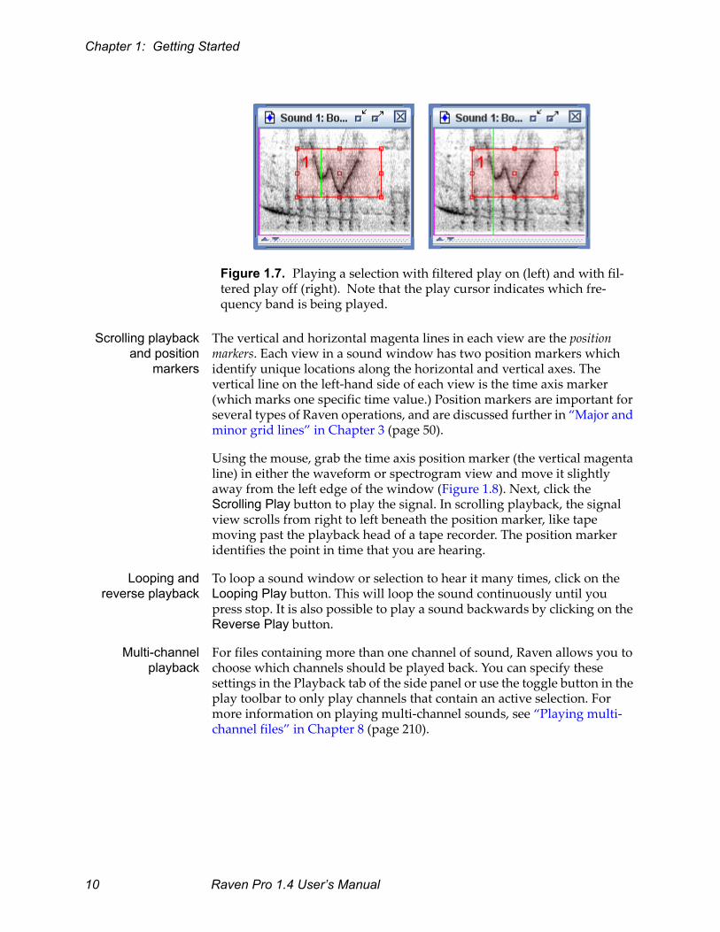
Figure 1.7
Figure 1.7. Playing a selection with filtered play on (left) and with fil-tered play off (right). Note that the play cursor indicates which fre-quency band is being played.
Scrolling playbackand position
markers
The vertical and horizontal magenta lines in each view are the position markers. Each view in a sound window has two position markers which identify unique locations along the horizontal and vertical axes. The vertical line on the left-hand side of each view is the time axis marker (which marks one specific time value.) Position markers are important for several types of Raven operations, and are discussed further in “Major and minor grid lines” in Chapter 3 (page 50).
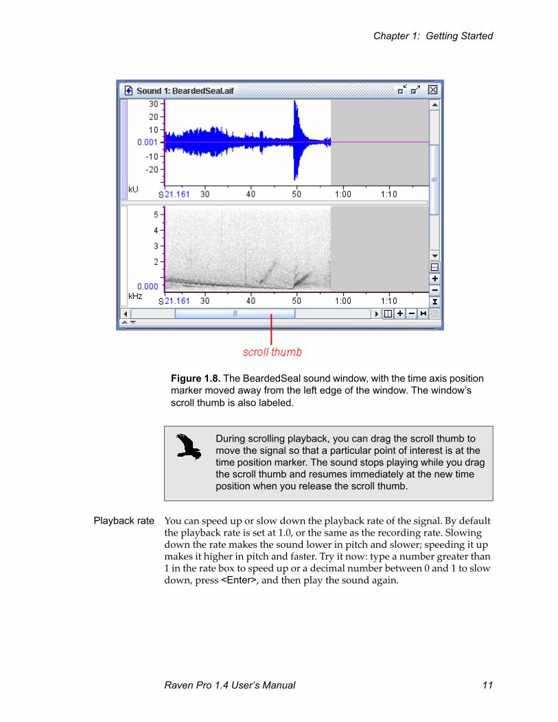
Using the mouse, grab the time axis position marker (the vertical magenta line) in either the waveform or spectrogram view and move it slightly away from the left edge of the window (Figure 1.8). Next, click the Scrolling Play button to play the signal. In scrolling playback, the signal view scrolls from right to left beneath the position marker, like tape moving past the playback head of a tape recorder. The position marker identifies the point in time that you are hearing.
Looping andreverse playback
To loop a sound window or selection to hear it many times, click on the Looping Play button. This will loop the sound continuously until you press stop. It is also possible to play a sound backwards by clicking on the Reverse Play button.
Multi-channelplayback
For files containing more than one channel of sound, Raven allows you to choose which channels should be played back. You can specify these settings in the Playback tab of the side panel or use the toggle button in the play toolbar to only play channels that contain an active selection. For more information on playing multi-channel sounds, see “Playing multi-channel files” in Chapter 8 (page 210).
10 Raven Pro 1.4 User’s Manual
Chapter 1: Getting Started
Figure 1.8 sound window, pos marker moved.
Figure 1.8. The BeardedSeal sound window, with the time axis position marker moved away from the left edge of the window. The window’s scroll thumb is also labeled.
Playback rate You can speed up or slow down the playback rate of the signal. By default the playback rate is set at 1.0, or the same as the recording rate. Slowing down the rate makes the sound lower in pitch and slower; speeding it up makes it higher in pitch and faster. Try it now: type a number greater than 1 in the rate box to speed up or a decimal number between 0 and 1 to slow down, press <Enter>, and then play the sound again.
During scrolling playback, you can drag the scroll thumb to move the signal so that a particular point of interest is at the time position marker. The sound stops playing while you drag the scroll thumb and resumes immediately at the new time position when you release the scroll thumb.
Raven Pro 1.4 User’s Manual 11
Chapter 1: Getting Started
Copying Part of a Sound
You can copy data in the active selection using commands on the Edit menu or standard keyboard equivalents. When you copy a selection, a copy of the selected data is put in the clipboard. The Paste command inserts the contents of the clipboard at the time of the active selection in the active sound window. If the active selection is a range (rather than a point), the clipboard contents replace the data in the selection. If there is no active selection, the Paste command is unavailable. Data on the clipboard can be pasted into the same sound window or into a different one.
Copying a selectionto a new sound
window
Create a new empty sound window by choosing File > New > Sound Window or by typing <Ctrl-N> (Windows, Linux) or <Command-N> (Mac OS). Next, make a selection in the ChestnutSidedWarbler.aif sound. Go to Edit > Copy to copy the data in the selection to the clipboard. Next, click on the new sound window to make it active and select Edit > Paste. You should now see the selection you made in the ChestnutSidedWarbler.aif sound appear in the new sound window (see Figure 1.9).
Figure 1.9 Copy a Selection
Figure 1.9. A selection from ChestnutSidedWarbler.aif copied into a new sound window.
12 Raven Pro 1.4 User’s Manual
Chapter 1: Getting Started
Copy a selection toan existing sound
With both sound windows open, make a new selection in the ChestnutSidedWarbler.aif signal. Copy this selection by choosing Edit > Copy, click in the middle of the second sound window to create an active selection, and paste the new selection there by choosing Edit > Paste (Figure 1.10).
Figure 1.10 Copying a Selection into a Sound
Figure 1.10. A second selection from ChestnutSidedWarbler.aif copied and pasted into the middle of the sound in the bottom window.
Saving All or Part of a Sound
You can save the active signal in a sound file, either in WAVE format (filename extension.wav) or in AIFF (Audio Interchange File Format, filename extension .aif) format. WAVE files can be opened by most other
If the sample rate of the data on the clipboard is not the same as that of the destination sound, Raven displays a warning and gives the option to continue or cancel the paste operation. If the sample rates do not match, the resulting sound will probably not be what you intended.
Raven Pro 1.4 User’s Manual 13
Chapter 1: Getting Started
programs that work with audio data. AIFF files can be opened by most Macintosh programs that work with audio data, and some programs on other platforms.
To choose a file format (WAVE or AIFF), and a sample size for the file to be saved, use the Files of Type drop-down menu in the Save As... dialog box (Figure 1.11). Choice of sample size is discussed in Appendix A, “Digital Representation of Sound”.
Saving a signal To save a sound, choose File > Save “Sound N” or File > Save “Sound N” As... . Choosing Save “Sound N” simply saves the sound under the same filename in the same location as the last time the sound was saved. If the sound has never been saved, Raven asks you to specify a location and name for the file. Choosing Save “Sound N” As... allows you to specify a new location and/or name for the file to be saved (Figure 1.11).
Figure 1.11 Save As... Dialog Box
Figure 1.11. This is the Save As... dialog box. After choosing a sound file or a sound selection to save, you can select a location for the file and specify a file name.
Files saved in WAVE or AIFF formats contain only the actual audio data. Information that is specifically for use with Raven (such as selection tables and layout parameters) is not saved in these files.
14 Raven Pro 1.4 User’s Manual
Chapter 1: Getting Started
To save a sequence of files as a list file, choose File > Save As List File. This saves a text file containing the names of the files and their order in the file sequence. Saving a file sequence as a list file allows you to quickly open the same sequence of files at a later time simply by opening the list file. For more on working with list files, see “Opening file sequences” in Chapter 7 (page 194).
Saving a selection After making a selection, within the ChestnutSidedWarbler.aif signal for example, choose File > Save Active Selection As... and you will see the Save As... dialog box (Figure 1.11). After entering a name for your selection and clicking Save, the active selection is saved into a new file by itself which can be opened at any time.
Saving Your Workspace
When you save a workspace, all aspects of Raven’s state are saved. By saving a workspace first, you can quit Raven and resume your work later exactly where you left off, even if you have many sound windows open.
Saving aworkspace
When you save a workspace, all information about Raven’s state is saved, including all open signals and the size and placement of their windows. To save the workspace, choose File > Save Workspace As... . Raven workspace files can be saved anywhere, and must have a filename extension of .wsp.
Opening aworkspace
To open a workspace file, choose File > Open Workspace... . If you have any sound windows open, Raven will warn you that they will be lost when the workspace file opens, and ask if you want to proceed. If there are signals open with unsaved changes, Raven gives you the opportunity to save them before opening the workspace file. Once the saved workspace opens, Raven is completely restored to its state at the time the workspace was saved.
You can also open a Raven workspace by dragging the work-space file’s icon from the computer’s desktop, a Windows Explorer window, or from a Mac Finder window, and dropping the icon on the Raven desktop.
Raven Pro 1.4 User’s Manual 15
Chapter 1: Getting Started
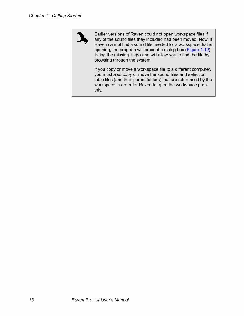
Earlier versions of Raven could not open workspace files if any of the sound files they included had been moved. Now, if Raven cannot find a sound file needed for a workspace that is opening, the program will present a dialog box (Figure 1.12) listing the missing file(s) and will allow you to find the file by browsing through the system.
If you copy or move a workspace file to a different computer, you must also copy or move the sound files and selection table files (and their parent folders) that are referenced by the workspace in order for Raven to open the workspace prop-erly.
16 Raven Pro 1.4 User’s Manual
Chapter 1: Getting Started
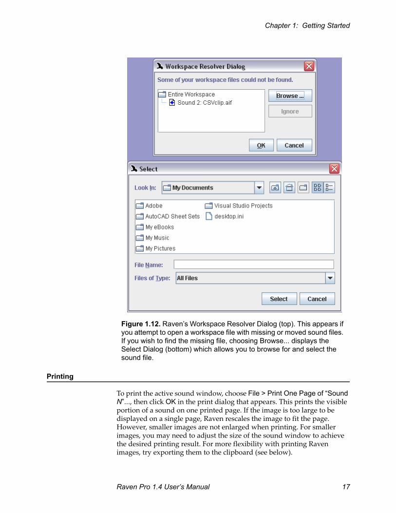
Figure 1.12 Workspace Resolver Dialog
Figure 1.12. Raven’s Workspace Resolver Dialog (top). This appears if you attempt to open a workspace file with missing or moved sound files. If you wish to find the missing file, choosing Browse... displays the Select Dialog (bottom) which allows you to browse for and select the sound file.
Printing
To print the active sound window, choose File > Print One Page of “Sound N”..., then click OK in the print dialog that appears. This prints the visible portion of a sound on one printed page. If the image is too large to be displayed on a single page, Raven rescales the image to fit the page. However, smaller images are not enlarged when printing. For smaller images, you may need to adjust the size of the sound window to achieve the desired printing result. For more flexibility with printing Raven images, try exporting them to the clipboard (see below).
Raven Pro 1.4 User’s Manual 17
Chapter 1: Getting Started
Alternatively, choosing File > Print Pages of “Sound N” will print the entire sound starting at the current location with each printed page displaying a length of sound equal to the visible section. Thus, choosing Print Pages is equivalent to printing one page of the sound, advancing forward by the length of the visible sound, printing another single page, and repeating this procedure until the end of the sound is reached. When printing a paged sound, Raven prints a full final page, which may result in some overlap between the last two images. If the entire sound is stored in memory, this overlap does not occur, and the final page is printed as a partial page.
By default, Raven prints in portrait orientation. To change to landscape orientation, choose File > Printer Page Setup, and choose Landscape orientation in the Page Setup dialog. The currently selected print orientation is indicated by the orientation of the page icon next to Printer Page Setup in the File menu.
Exporting images tofiles
To save an image of all or part of the Raven window as a graphics file, choose File > Export Image Of. A submenu appears showing the graphics objects that Raven can copy: the entire Raven window, the active sound window, all views within the active sound window, or each individual view within the active window. Choose whichever object you want to export from the submenu. In the Export Image dialog box that appears, choose a graphics file format. Any of the four graphics objects can be saved in PNG, TIFF, JPEG, or BMP format. Views can also be saved in Encapsulated Post Script (EPS) format, but image scaling does not work for this format.
Copying images tothe clipboard
To copy an image of all or part of the Raven window so that you can paste it into a document in another program, choose Edit > Copy Image Of. A submenu appears showing the four graphics objects that Raven can copy: the entire Raven window, the active sound window, all views within the active sound window, or the active view of the active window. Choose whichever object you want to copy from the submenu. The copied image can be pasted into documents in any program that works with graphic images.
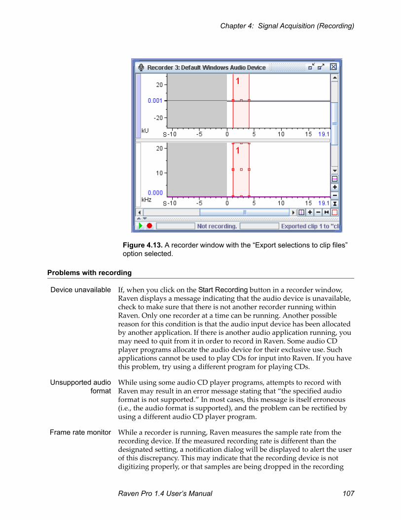
Recording a sound (acquiring input)
Raven obtains its audio input from an audio source (e.g., a tape recorder, CD player, or microphone) connected to a particular port on an audio
If you click on the printer Properties button in the Print dialog, a dialog appears that contains another set of controls for choosing page orientation. These controls may not correctly display or allow you to change the actual page orientation. To change the page orientation, always use File > Printer Page Setup.
18 Raven Pro 1.4 User’s Manual
Chapter 1: Getting Started
input device installed on your computer (e.g., microphone or line input port of an internal sound card or USB sound input device).
Raven can acquire a signal directly to a file, to a sequence of files, or to memory only (without saving to disk). While Raven is acquiring input you can see multiple views— waveforms, spectrograms, spectrogram slices— scroll by in real time.
This section covers acquiring a signal to memory. Recording to a file or file sequence is discussed in Chapter 4, “Signal Acquisition (Recording)” and also covers decimating the input signal (acquiring it at a lower effective sample rate).
Selecting an audioinput device
You use controls supplied by the operating system to choose and configure the audio input device that Raven will use. Appendix A, “Digital Representation of Sound” discusses how to choose a particular audio input device on each operating system. Before proceeding further, you should refer to the appendix to ensure that your system is properly configured.
Connect an audio source (e.g., tape recorder, CD player, or microphone) to the appropriate port of the audio input device you selected.
Create newrecorder
To ready Raven for acquiring a signal, click on the Record button on the file toolbar (Figure 1.13). You can also press <Ctrl-R> (Windows, Linux) or <Command-R> (Mac OS), or choose File > New > Recorder... Doing so will display the Configure New Recorder dialog box (Figure 1.14).
Figure 1.13 Record button
Figure 1.13. The Record button, located in the file toolbar of the Raven desktop.
Raven Pro 1.4 User’s Manual 19
Chapter 1: Getting Started
Figure 1.14. New Recorder dialog.
Figure 1.14. Raven’s Configure New Recorder dialog box.
Use fields in the Configure New Recorder box to acquire the signal to memory or to one or more files, to choose which input device and device configuration to use, and to specify how to display the sound while it’s being acquired. For now, to give you a feel for Raven’s capabilities, we’ll go over how to record sounds to memory (without saving them to disk) and what you can do with the signal as it’s coming in. Chapter 4, “Signal Acquisition (Recording)” explains in detail what each of the fields in this dialog box do. For now, just leave all the fields as they are and click OK or press <Enter>.
The RecorderWindow
When you click OK or press <Enter> in the Configure New Recorder dialog box, a new recorder window appears on the Raven desktop (Figure 1.15). A recorder window looks and behaves like any other Raven sound window except that it has additional controls displayed in the status bar at the bottom of the window.
20 Raven Pro 1.4 User’s Manual
Chapter 1: Getting Started
Figure 1.15. Recorder window (to memory).
Figure 1.15. A new Recorder window, configured for recording one channel to memory.
Starting andstopping the real-
time signal display
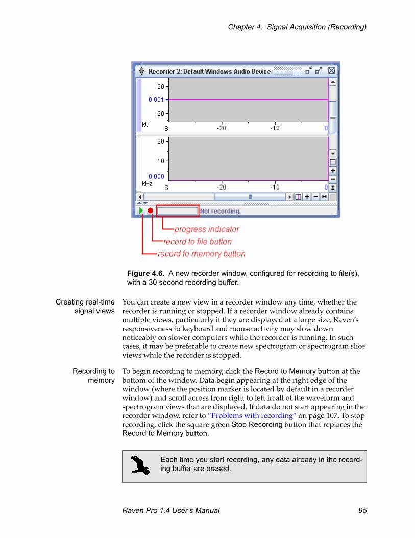
Click the triangular green Record-to-Memory button (Figure 1.15) to start a real-time scrolling waveform display in the recorder window. When you start providing an audio signal (by starting playback of a tape or CD, or by speaking into a microphone), you should see a waveform appear at the right edge of the waveform window and scroll across to the left. The Record-to-Memory button is replaced by a square Stop Recording button, and the status field next to the button displays the message “Recording to memory”.
When the waveform reaches the left edge, the oldest data are discarded to make room for the newest data. Time counts up from the right side and scrolls across the view. Clicking the Stop Recording button stops recording. If you click the button to start recording again, Raven clears the Recorder window before beginning to display the new signal.
By default, when recording to memory only, Raven records into a 30-second sound buffer. You can specify a longer sound buffer when configuring the recorder (see “Buffer Size” in Chapter 4 (page 84)).
While recording isstopped…
When you stop a recording, the most recent part of the signal remains displayed on the screen. You can do anything with this signal fragment
Raven Pro 1.4 User’s Manual 21
Chapter 1: Getting Started
that you can do with a signal in any other sound window: save it, make selections from it, copy from it, print it— whatever you like. Remember that if you have been recording for a while you will only have the latest part of the signal to work with (only what can be displayed), and not the entire signal from the point at which you began recording.
More aboutrecording
Chapter 4, “Signal Acquisition (Recording)” covers the recording process in more depth. Read that chapter to find out:•how to select and configure your input device•how to record to a file or a sequence of files•how to incorporate date- and time-stamps into names of acquired files•how to acquire signals at lower sample rates than those available from an
audio input device (signal decimation)•other operations to perform while recording
22 Raven Pro 1.4 User’s Manual
Chapter 2 The Raven Window
About this chapter
In this chapter you’ll learn about the three main parts of the Raven Window and how to adjust the appearance of the application. Topics include:•the Menu bar•the Toolbars•keyboard shortcuts •the Side panel and mouse measurement field•changing the appearance of the Raven Window
The Menu bar
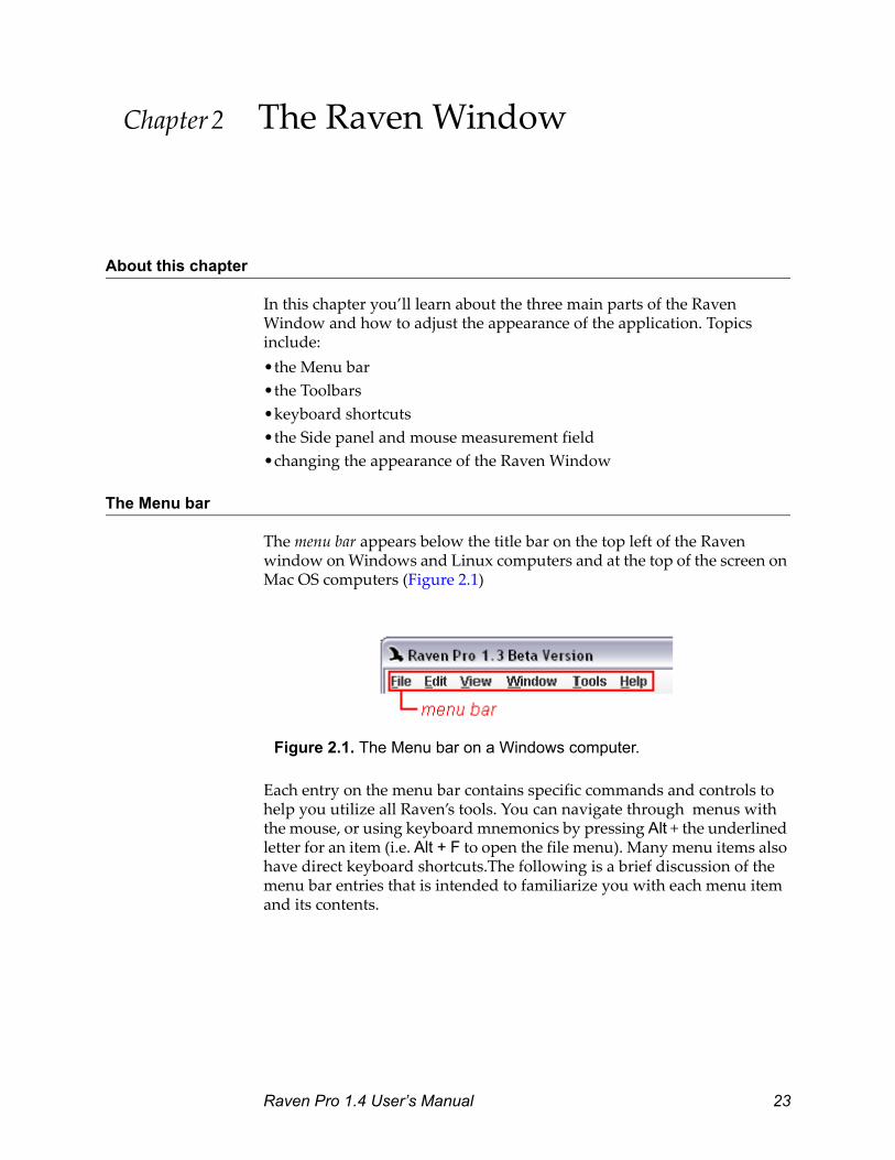
The menu bar appears below the title bar on the top left of the Raven window on Windows and Linux computers and at the top of the screen on Mac OS computers (Figure 2.1)
Figure 2.1 The Menu bar
Figure 2.1. The Menu bar on a Windows computer.
Each entry on the menu bar contains specific commands and controls to help you utilize all Raven’s tools. You can navigate through menus with the mouse, or using keyboard mnemonics by pressing Alt + the underlined letter for an item (i.e. Alt + F to open the file menu). Many menu items also have direct keyboard shortcuts.The following is a brief discussion of the menu bar entries that is intended to familiarize you with each menu item and its contents.
Raven Pro 1.4 User’s Manual 23
Chapter 2: The Raven Window
The File menu Figure 2.2 The File menu
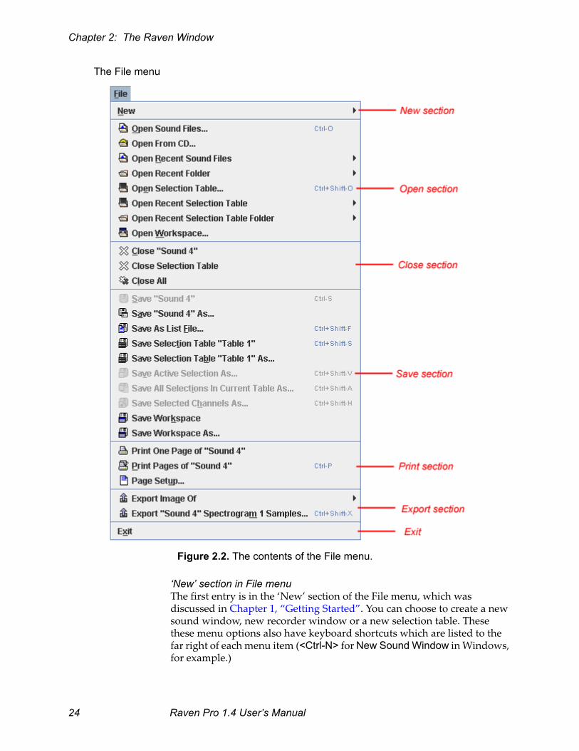
Figure 2.2. The contents of the File menu.
‘New’ section in File menuThe first entry is in the ‘New’ section of the File menu, which was discussed in Chapter 1, “Getting Started”. You can choose to create a new sound window, new recorder window or a new selection table. These these menu options also have keyboard shortcuts which are listed to the far right of each menu item (<Ctrl-N> for New Sound Window in Windows, for example.)
24 Raven Pro 1.4 User’s Manual
Chapter 2: The Raven Window
‘Open’ section in File menuThe next section contains the ‘Open’ options, some of which were discussed in Chapter 1, “Getting Started”. You can choose to open a sound from an existing file or CD, or choose a recently used file or another sound from a recently used folder. You can also open a saved selection table or workspace (see discussion in “The Selection Table” in Chapter 6 (page 150)), recent selection table, or another selection table from a recently used folder. Again, some of these ‘Open’ options have keyboard shortcuts listed to the far right if you prefer using those.
‘Close’ section in File menuThe ‘Close’ section contains commands used to close files and other items that you were working with. You can choose to close an individual sound file, close a selection table (more on these in “Selection Tables” in Chapter 6 (page 150)) or to simply close all the files open on the Raven desktop.
‘Save’ section in File menuThere are many options for saving your work, several of which were mentioned in Chapter 1, “Getting Started”. In the Save section, you can save sound files, selection tables, and workspaces that have already been saved somewhere. To save items for the first time, or to save a file under a new name, choose Save as... “Saving as...” is available for sound files, selection tables, active selections, all selections, selected channels, and workspaces.
‘Print’ section in File menuIn the ‘Print’ section, you can choose to print a sound file, print sections of the file, or make changes to the page setup which will adjust the printed output. Remember that the printer Properties button in the Print dialog may not correctly display or change the page orientation; page settings should only be adjusted through the File > Page Setup... menu item.
‘Export’ section in File menuThis section has options for exporting images (discussed in “Exporting images to files” in Chapter 1 (page 18)) as well as exporting samples from sound file views (more on this in “Export output and text file content” in Chapter 6 (page 179)).
‘Exit’ in File menuWhen you are finished using Raven, you can exit the application by choosing File > Exit from the menu bar or by clicking the system close icon in the window title bar.
Raven Pro 1.4 User’s Manual 25
Chapter 2: The Raven Window
The Edit menu Figure 2.3 The Edit menu
Figure 2.3. The contents of the Edit menu.
Undo/Redo items in Edit menuAfter performing an edit operation, you may wish to undo your change. To revert back to the previous state, choose Undo. In some cases, you may wish to reapply a change that was just revoked. To remake a change that was undone, choose Redo. Note that the action you will be undoing/redoing will also be listed in the menu (for example, Undo Filter or Redo Paste).
‘Editing’ section in Edit menuThe main section of the Edit menu contains commands to Cut or Copy a selection to the clipboard, Paste a selection from the clipboard, or Delete a selection. These editing options all deal with sound samples, and more information about these processes can be found in “Editing a sound” in Chapter 6 (page 146).
Filter/Amplify items in Edit menuAlso in the Edit menu, you can choose to Filter and/or Amplify parts of signals. More details on these processes can be found in “Filtering and amplifying sounds” in Chapter 6 (page 147).
Copy Image OfSimilar to the Export Image Of... function in the File menu, you can choose to copy image information to the clipboard from within the Edit menu. Selecting Copy Image Of allows you to copy an image of the entire Raven window, a particular sound window, or certain views within a sound window to the clipboard for use in other applications.
Select All
26 Raven Pro 1.4 User’s Manual
Chapter 2: The Raven Window
Choosing this menu item selects all information displayed in the Raven sound window. In cases where you need to make changes or edit all the information displayed, this bypasses the time and effort required to individually select everything. Also, if the sound window is zoomed to a subset of the entire sound, only the visible subset of the current view will be selected.
Preferences
This item opens the Raven preferences file for editing. The preferences file stores many of Raven’s presets and default settings. This file is also saved in the Raven program directory as RavenPreferences.txt. For more information on editing the preferences file, see “About Raven preferences” in Chapter 11 (page 299).
Raven Pro 1.4 User’s Manual 27
Chapter 2: The Raven Window
The View menu Figure 2.4
Figure 2.4. The contents of the View menu.
Basic commandsFrom this menu, you can select which toolbars are visible and you can lock their positions. You can create a new view or work with window presets (see more on these topics in Chapter 3, “Sound Windows: Visibility, Views,
28 Raven Pro 1.4 User’s Manual
Chapter 2: The Raven Window
Linkage, & Navigation” and Chapter 11, “Customizing Raven”). You can choose to apply the view settings of a sound window to all other open windows and you can also adjust configuration settings of a recorder.
‘View’ section in View menuThis section contains commands that allow you to adjust views by hiding them, deleting them, or moving them up and down within a sound window. More information regarding views is discussed in Chapter 3, “Sound Windows: Visibility, Views, Linkage, & Navigation”.
UnlinkingYou can choose to unlink views within a sound window by selecting this submenu. Details on how this works and when you might want to do this can be found in “Linking and unlinking views” in Chapter 3 (page 62).
Configure viewViews can be adjusted in several ways. The color scheme can be changed, and the display axes of the view can be adjusted or hidden. You can also choose which, if any, grids to display in each view. For more information on how to adjust views, see Chapter 3, “Sound Windows: Visibility, Views, Linkage, & Navigation”. This section may also have more menu items available depending on the active view (spectrogram views, for example, will have entries allowing you to adjust spectrogram parameters and smoothing.)
DetectorsYou can select and run interactive detectors by choosing this item.
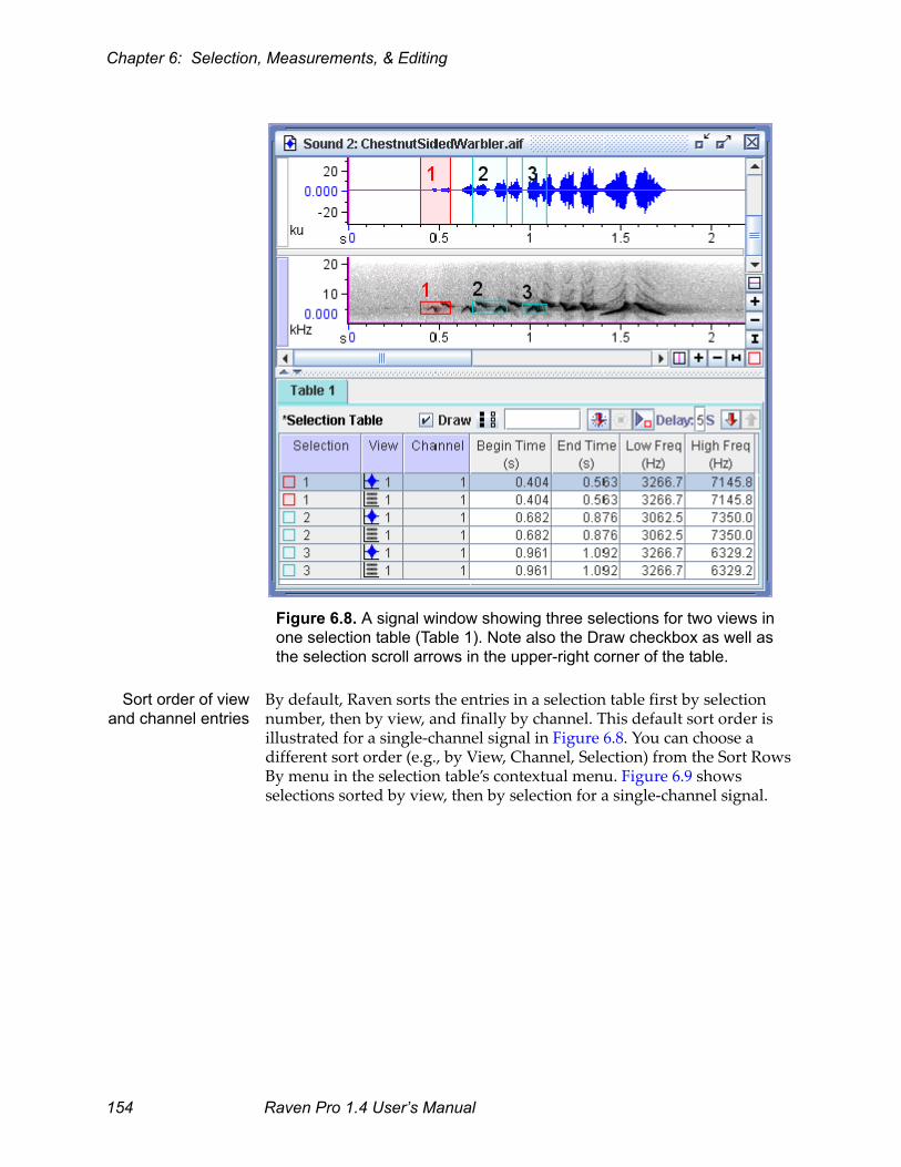
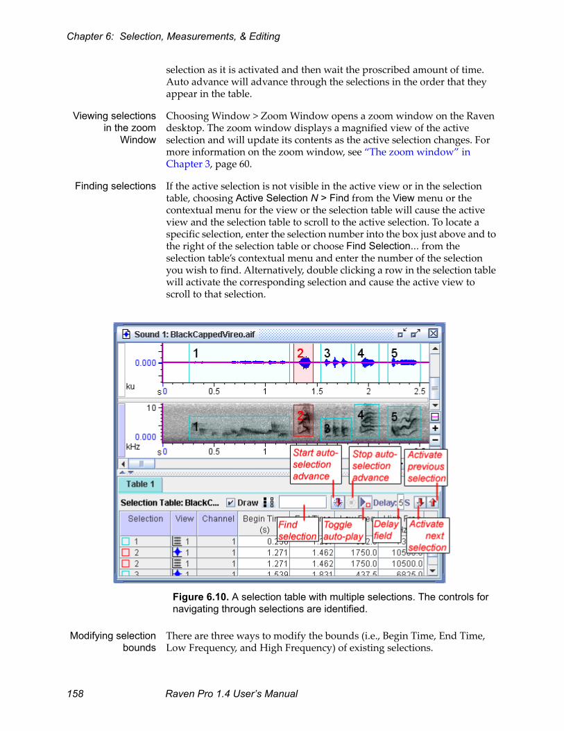
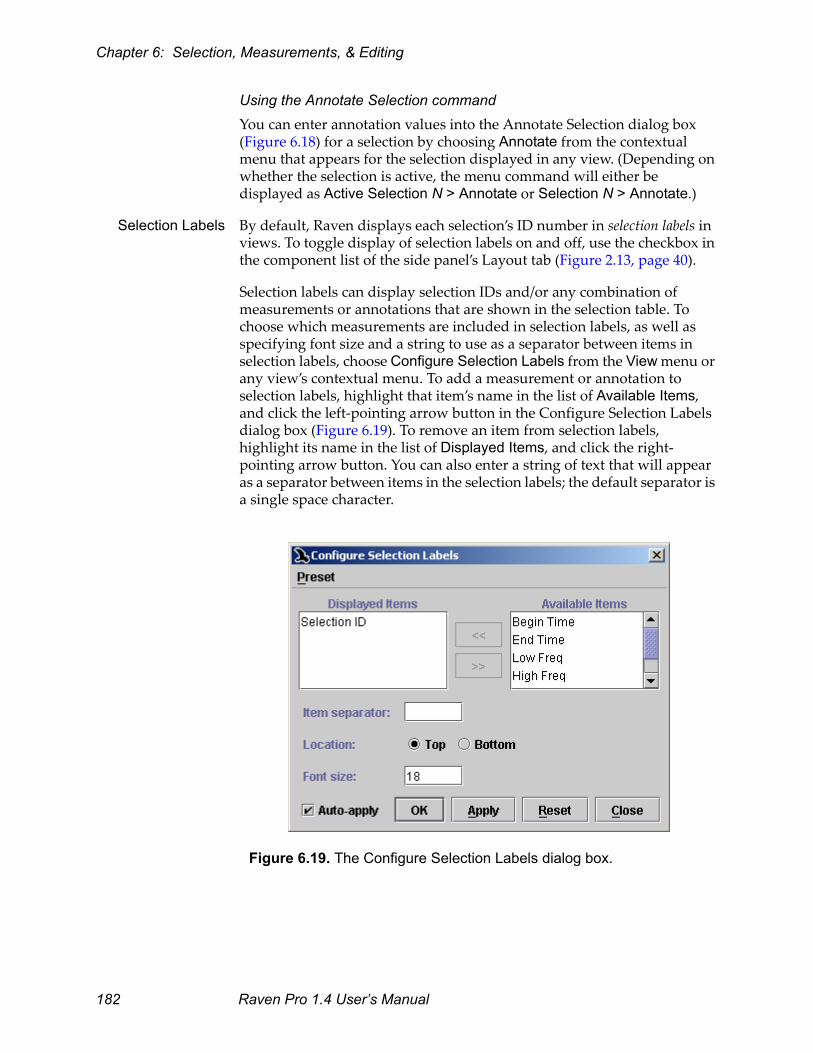
Measurements, annotations, and labelsYou can choose to make measurements and annotations of displayed information in the selection table, choose which selections to display, and how these selections are labeled. More information on this can be found in Chapter 6, “Selections: Measurements, Annotations, & Editing”.
SelectionsAfter making selections, there are many things you can do with them, including copying, clearing, and pasting them. Some of these commands can be found in the Active Selection submenu. This section also includes ways to locate or highlight a particular selection in the selection table. Basic selection copying was discussed in “Copying Part of a Sound” in Chapter 1 (page 12) and you can find more details on selections and various ways to work with them in Chapter 6, “Selections: Measurements, Annotations, & Editing”.
Raven Pro 1.4 User’s Manual 29
Chapter 2: The Raven Window
The Window menu Figure 2.5 Window menu
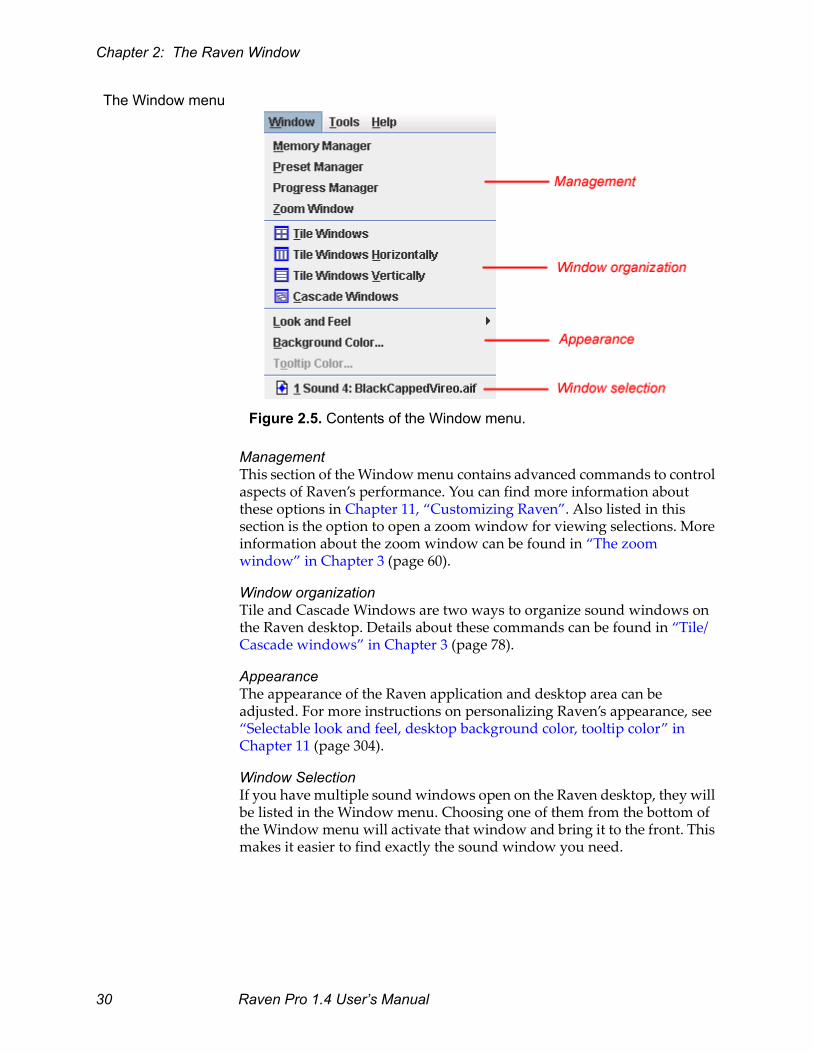
Figure 2.5. Contents of the Window menu.
ManagementThis section of the Window menu contains advanced commands to control aspects of Raven’s performance. You can find more information about these options in Chapter 11, “Customizing Raven”. Also listed in this section is the option to open a zoom window for viewing selections. More information about the zoom window can be found in “The zoom window” in Chapter 3 (page 60).
Window organizationTile and Cascade Windows are two ways to organize sound windows on the Raven desktop. Details about these commands can be found in “Tile/Cascade windows” in Chapter 3 (page 78).
AppearanceThe appearance of the Raven application and desktop area can be adjusted. For more instructions on personalizing Raven’s appearance, see “Selectable look and feel, desktop background color, tooltip color” in Chapter 11 (page 304).
Window SelectionIf you have multiple sound windows open on the Raven desktop, they will be listed in the Window menu. Choosing one of them from the bottom of the Window menu will activate that window and bring it to the front. This makes it easier to find exactly the sound window you need.
30 Raven Pro 1.4 User’s Manual
Chapter 2: The Raven Window
The Tools menu Figure 2.6
Figure 2.6. Contents of the Tools menu.
The items in the Tools menu are advanced ways to work with data in sound files. For information on using the correlation tool, please refer to Chapter 9, “Correlation”. For help with making detections, see Chapter 10, “Detection”. And to perform batch operations on many sounds at once, see “Batch Operations” in Chapter 7 (page 192).
The Help menu Figure 2.7 Help menu
Figure 2.7. Contents of the Help menu.
DocumentationThis section of the Help menu contains links to documentation for the Raven software. You can access the entire Raven User’s Manual by selecting the first option or you can choose to view the “What’s New” document. You can visit the Raven web site, view frequently asked
Raven Pro 1.4 User’s Manual 31
Chapter 2: The Raven Window
questions, or read the Raven license agreement. You can also access the Raven Help Forum which is a great tool for users.
FeedbackBy selecting the Email Feedback option, you can submit comments, bug reports, support requests, and other feedback to the Raven software team via email. For more information on contacting the Raven software team and how to use the Email Feedback form, please see “Contacting the Raven development and support team” in Chapter 11 (page 315).
UpdatesPeriodically, the Raven software team releases updates and changes to the Raven application. You can check for and read about these updates in this section of the Help menu. You can also download the QuickTime installer (more on this process can be found in “Opening sounds in different file formats” in Chapter 1 (page 6)).
AboutSelecting About Raven... allows you to view information regarding copyright information, thanks, and credits for the application.
The Toolbars
There are five main toolbars in Raven. You can control whether a toolbar is displayed or hidden by selecting View > Toolbars > <Toolbar Name>. If the toolbar has a checked box next to its name, it is already visible. If the box is empty, the toolbar is hidden. In the same menu (View > Toolbars) you can also choose to lock or unlock the toolbars. If the icon is a locked padlock, the toolbars are locked and you will be unable to move or otherwise adjust their positions. Unlocking the toolbars (denoted by an unlocked padlock) allows you to move the toolbars around if you so desire.
The file toolbar The file toolbar is located underneath the menu bar, across the top of the Raven window (see Figure 2.8). It contains buttons allowing you to create new items, open existing items, save items, and print (in addition to adjusting the page setup for printing purposes). Since this section is intended only to introduce the contents of the toolbar, specific information about the commands and their functionality can be found throughout this manual.
32 Raven Pro 1.4 User’s Manual
Chapter 2: The Raven Window
Figure 2.8 file toolbar
Figure 2.8. The file toolbar.
New Recorder, New Sound Window, New Selection TableThe first three buttons in the file toolbar create new items (recorders, sound windows, or selection tables). You can also create these items by accessing the File menu (“‘New’ section in File menu” on page 24).
Open Sound Files, Open CD, Open Selection Table, Open WorkspaceThe next set of four buttons allows you to open various items (sounds from files or CD, selection tables, or saved workspaces). You can also open these items from the File menu (“‘Open’ section in File menu” on page 25).
Save Sound, Save Sound File As..., Save Selection Table, Save SelectionTable, Save Active Selection As..., Save All Selections As..., Save SelectedChannels As..., Save WorkspaceThere are 7 buttons with various Save functionality in the toolbar. You can save certain items through the File menu as well (“‘Save’ section in File menu” on page 25).
Print Sound, Page SetupIf you’d like to print a sound, or adjust the page settings before printing, the last two buttons provide an easy way to do so. Of course, you can always go through the File menu to access these options as well (“‘Print’ section in File menu” on page 25).
The edit toolbar The edit toolbar is typically located underneath the file toolbar (although, if you unlock the toolbars and move them around, the location could be different). This toolbar contains buttons related to editing, filtering, and amplifying sounds and selections. More information on these topics can be found in Chapter 6, “Selections: Measurements, Annotations, & Editing”.
Raven Pro 1.4 User’s Manual 33
Chapter 2: The Raven Window
Figure 2.9
Figure 2.9. The edit toolbar.
Undo, Redo, Cut, Copy, Paste, Delete, Select AllThese buttons contain basic editing commands that can also be applied by selecting the Edit menu (“Undo/Redo items in Edit menu” on page 26 and “‘Editing’ section in Edit menu” on page 26).
Raven Preferences
This button provides a link to open and edit the Raven preferences file, which stores many of Raven’s presets and default settings. This file is also saved in the Raven program directory as RavenPreferences.txt. For more information on editing the preferences file, see “About Raven preferences” in Chapter 11 (page 299).
Filter Around Active Selection, Filter Out Active Selection, Filter ActiveSelection With..., Filter Around All, Filter Out All, Filter All With..., Amplify...To quickly perform filtering or amplification, you can use these buttons. Alternately, you can perform the same tasks by accessing the Edit > Band Filter menu or Edit > Amplify item (“Filter/Amplify items in Edit menu” on page 26) if you prefer.
The view toolbar This toolbar contains buttons that will create new views as well as adjust the way sound windows and views will appear. For more information on these topics, see Chapter 3, “Sound Windows: Visibility, Views, Linkage, & Navigation”.
34 Raven Pro 1.4 User’s Manual
Chapter 2: The Raven Window
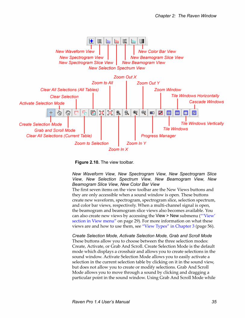
Figure 2.10 the view toolbar
Figure 2.10. The view toolbar.
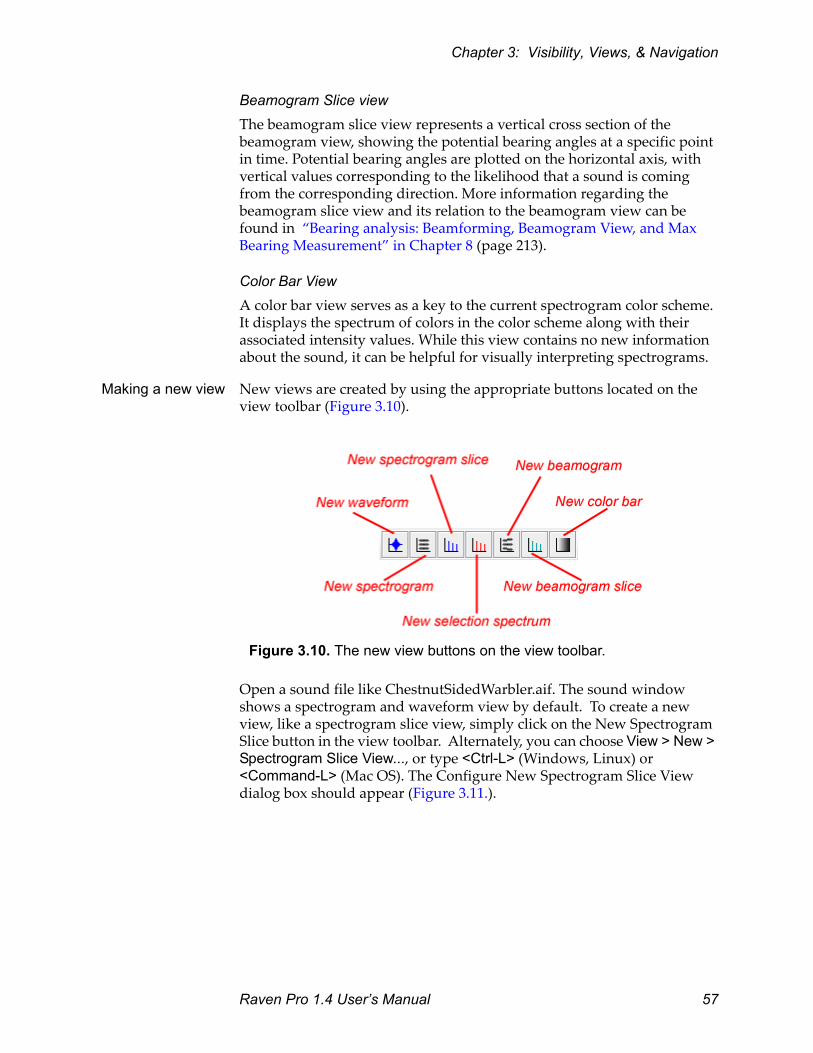
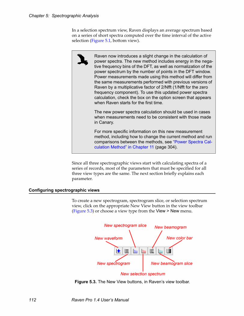
New Waveform View, New Spectrogram View, New Spectrogram SliceView, New Selection Spectrum View, New Beamogram View, NewBeamogram Slice View, New Color Bar ViewThe first seven items on the view toolbar are the New Views buttons and they are only accessible when a sound window is open. These buttons create new waveform, spectrogram, spectrogram slice, selection spectrum, and color bar views, respectively. When a multi-channel signal is open, the beamogram and beamogram slice views also becomes available. You can also create new views by accessing the View > New submenu (“‘View’ section in View menu” on page 29). For more information on what these views are and how to use them, see “View Types” in Chapter 3 (page 56).
Create Selection Mode, Activate Selection Mode, Grab and Scroll ModeThese buttons allow you to choose between the three selection modes: Create, Activate, or Grab And Scroll. Create Selection Mode is the default mode which displays a crosshair and allows you to create selections in the sound window. Activate Selection Mode allows you to easily activate a selection in the current selection table by clicking on it in the sound view, but does not allow you to create or modify selections. Grab And Scroll Mode allows you to move through a sound by clicking and dragging a particular point in the sound window. Using Grab And Scroll Mode while
Raven Pro 1.4 User’s Manual 35
Chapter 2: The Raven Window
holding down the shift key allows you to scroll horizontally while locking the vertical axis.
Clear Selection, Clear All Selections, Zoom to Selection, Zoom to All, ZoomIn X, Zoom Out X, Zoom In Y, Zoom Out YIf you want to quickly clear a single selection, or clear all selections in a sound window, you can use the first two buttons on the left. You can also access these commands at the bottom of the View menu, or by using the selection context menu. If you’d like to adjust the appearance of a particular view, you can use the zoom buttons in the toolbar. The same functionality can be achieved by using the zoom buttons on the sound window itself (“Changing view scales by zooming” in Chapter 3 (page 53)).
Progress Manager, Zoom WindowTo use Raven’s progress manager to view the progress of background tasks, use the Progress Manager button. For more information, see “Progress Manager” in Chapter 7 (page 192). The Zoom Window button can be used to examine a selection; see “The zoom window” in Chapter 3 (page 60).
Tile Windows, Tile Windows Horizontally, Tile Windows Vertically, CascadeWindowsIf you want to change how the sound windows are displayed on the desktop, you can choose to tile or cascade them using the four buttons on the far right. These commands can also be found listed in the Window menu (“Tile/Cascade windows” in Chapter 3 (page 78)).
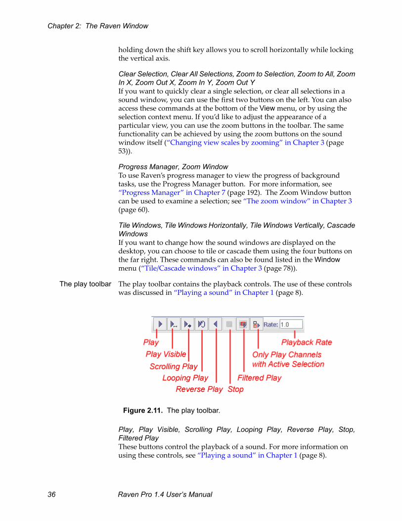
The play toolbar The play toolbar contains the playback controls. The use of these controls was discussed in “Playing a sound” in Chapter 1 (page 8).
Figure 2.11
Figure 2.11. The play toolbar.
Play, Play Visible, Scrolling Play, Looping Play, Reverse Play, Stop,Filtered PlayThese buttons control the playback of a sound. For more information on using these controls, see “Playing a sound” in Chapter 1 (page 8).
36 Raven Pro 1.4 User’s Manual
Chapter 2: The Raven Window
Only Play Channels with Active SelectionWhen playing multi-channel files, you can opt to only play channels that contain the active selection. For more information on playing multi-channel files, see “Playing multi-channel files” in Chapter 8 (page 210).
Playback RateThis controls the speed at which a sound is played. You can speed up or slow down the playback rate of the signal. By default the playback rate is set at 1.0, or the same as the recording rate. Slowing down the rate makes the sound lower in pitch and slower; speeding it up makes it higher in pitch and faster.
The spectrogramtoolbar
The spectrogram toolbar gives you access to making quick adjustments to the appearance of spectrogram displays. For more detailed information on spectrograms, see Chapter 5, “Spectrographic Analysis”.
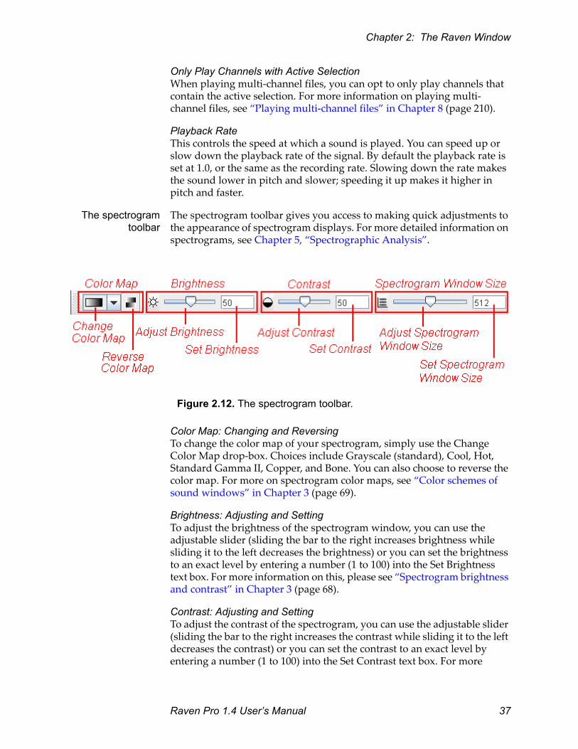
Figure 2.12 the spectrogram toolbar
Figure 2.12. The spectrogram toolbar.
Color Map: Changing and ReversingTo change the color map of your spectrogram, simply use the Change Color Map drop-box. Choices include Grayscale (standard), Cool, Hot, Standard Gamma II, Copper, and Bone. You can also choose to reverse the color map. For more on spectrogram color maps, see “Color schemes of sound windows” in Chapter 3 (page 69).
Brightness: Adjusting and SettingTo adjust the brightness of the spectrogram window, you can use the adjustable slider (sliding the bar to the right increases brightness while sliding it to the left decreases the brightness) or you can set the brightness to an exact level by entering a number (1 to 100) into the Set Brightness text box. For more information on this, please see “Spectrogram brightness and contrast” in Chapter 3 (page 68).
Contrast: Adjusting and SettingTo adjust the contrast of the spectrogram, you can use the adjustable slider (sliding the bar to the right increases the contrast while sliding it to the left decreases the contrast) or you can set the contrast to an exact level by entering a number (1 to 100) into the Set Contrast text box. For more
Raven Pro 1.4 User’s Manual 37
Chapter 2: The Raven Window
information on this, please see “Spectrogram brightness and contrast” in Chapter 3 (page 68).
Spectrogram Window Size: Adjusting and SettingThe window size parameter controls the length of each data record that is analyzed to create each of the individual spectra that together constitute the spectrogram. The default unit for this measurement is number of samples. For more information on window size, please see “Window size” in Chapter 5 (page 116).
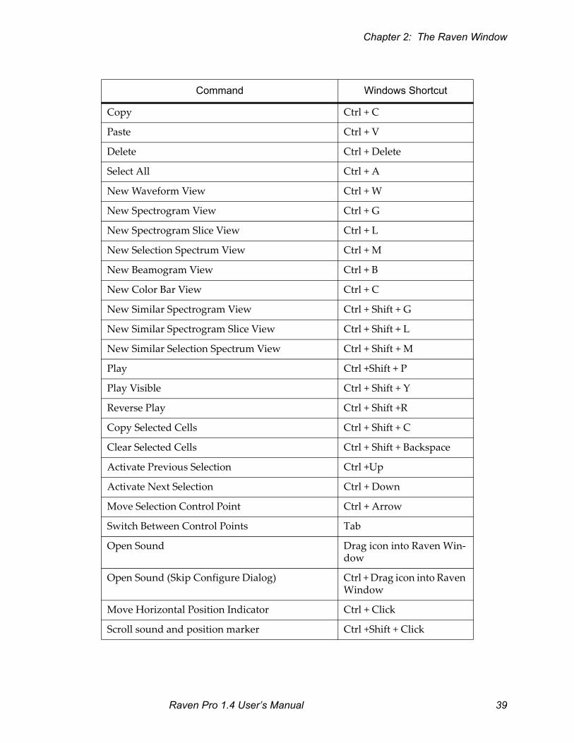
Keyboard Shortcuts
Many of the functions listed in the menus and toolbars also have keyboard shortcuts associated with them. A list of these functions, and their corresponding shortcuts in Windows is provided below. The shortcuts for Mac are the same as those for Windows, but use the Command key in place of Ctrl.
Command Windows Shortcut
New Sound Window Ctrl + N
New Recorder Ctrl + R
New Selection Table Ctrl + T
New Selection Table (with Measurements) Ctrl + Shift + T
Open Sound Files Ctrl + O
Open Selection Table Ctrl + Shift + O
Save Sound N Ctrl + S
Save As List File... Ctrl + Shift + F
Save Selection Table Ctrl + Shift + S
Save Active Selection As... Ctrl + Shift + V
Save All Selections in Current Table As... Ctrl + Shift + A
New Similar Spectrogram Slice View Ctrl + Shift + L
New Similar Selection Spectrum View Ctrl + Shift + M
Play Ctrl +Shift + P
Play Visible Ctrl + Shift + Y
Reverse Play Ctrl + Shift +R
Copy Selected Cells Ctrl + Shift + C
Clear Selected Cells Ctrl + Shift + Backspace
Activate Previous Selection Ctrl +Up
Activate Next Selection Ctrl + Down
Move Selection Control Point Ctrl + Arrow
Switch Between Control Points Tab
Open Sound Drag icon into Raven Win-dow
Open Sound (Skip Configure Dialog) Ctrl + Drag icon into Raven Window
Move Horizontal Position Indicator Ctrl + Click
Scroll sound and position marker Ctrl +Shift + Click
Command Windows Shortcut
Raven Pro 1.4 User’s Manual 39
Chapter 2: The Raven Window
The Side Panel
The left side of the Raven window holds the side panel, which contains six tabs: Layout, Linkage, Selection, Playback, Detection, and Information. By default, the side panel opens to the Layout tab; see Figure 2.13.
Figure 2.13 The Side Panel
Figure 2.13. A general view of the side panel, with basic layout features outlined in red.
Docking controls Clicking on these arrows controls the visibility of the side panel. If you choose the arrow pointing toward the left (at the top for Windows and Linux users, or at the bottom for Mac OS) the side panel will be docked or hidden, and you will be unable to view its contents. If you select the arrow pointing toward the right, the side panel will become undocked and will
40 Raven Pro 1.4 User’s Manual
Chapter 2: The Raven Window
become visible again. When the side panel is docked or undocked, any maximized sound windows will be resized to occupy the entire Raven desktop. Similar docking control arrows appear throughout the application in cases where panels can be docked to provide more viewing room for other information.
Vertical separatorbar
The gray shaded bar to the right of the side panel can be moved to the left and right to control the width of the side panel itself. To resize the side panel, simply click your mouse over the control bar and, while holding the mouse button, drag the mouse to the right or left.
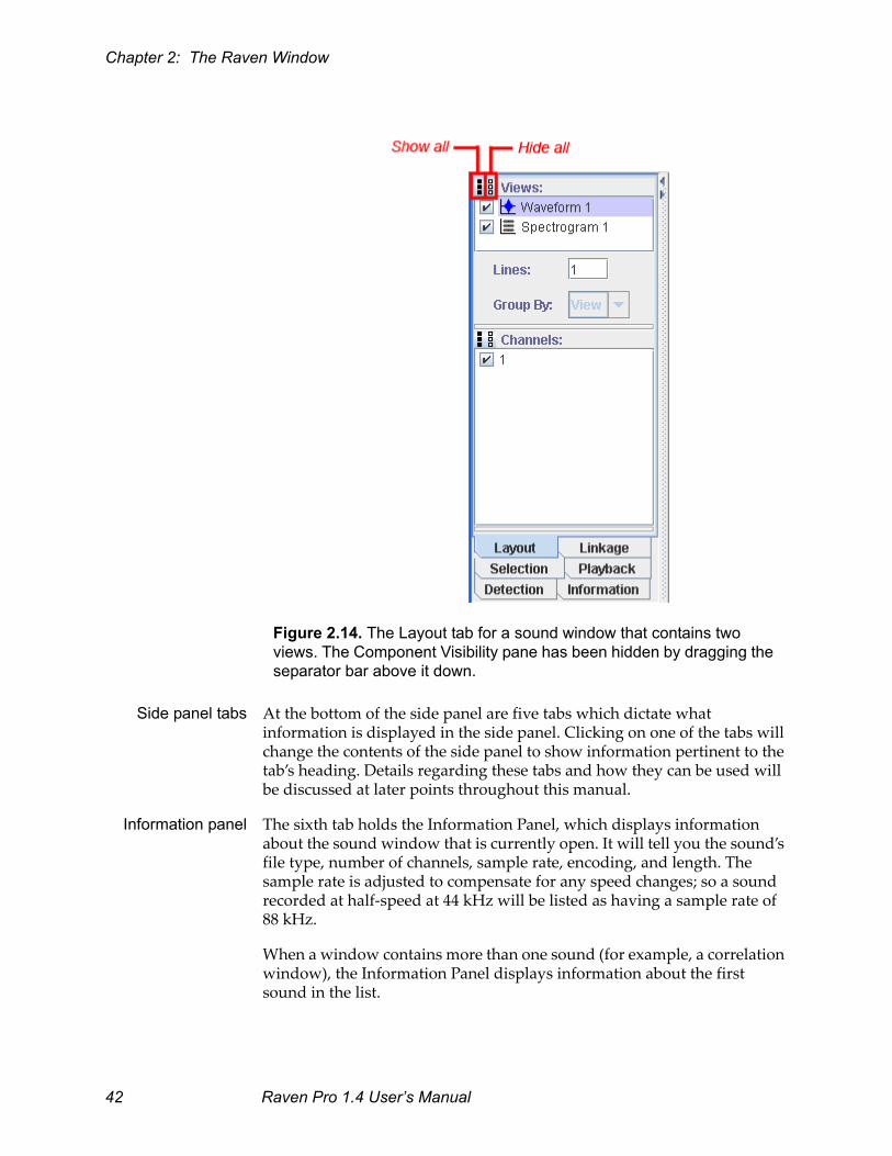
Show all/Hide all The side panel contains different sections of information. Each section in the panel contains a list of items. When a checkbox next to an item is checked, that item will be shown in the active sound window on the Raven desktop. For example, if you open ChestnutSidedWarbler.aif, the items listed under the View section in the side panel should be ‘Waveform 1’ and ‘Spectrogram 1’, with both checkboxes checked. This means that both the waveform and spectrogram views are shown in the ChestnutSidedWarbler.aif sound window. For a brief review of what the sound window looks like, please refer to “Understanding the Sound Window” in Chapter 1 (page 7).
Sometimes, you may want to hide all the items listed in a side panel section. To do this, select the Hide all button (the three white, ‘empty’ boxes). This will uncheck the checkboxes and will hide these items from being seen in the sound window. To show all the items listed in a side panel section, select the Show all button (the three black boxes) and this will make the items visible in the sound window. See Figure 2.14. for more information on hiding and showing all components.
Raven Pro 1.4 User’s Manual 41
Chapter 2: The Raven Window
Figure 2.14.. Layout tab
Figure 2.14. The Layout tab for a sound window that contains two views. The Component Visibility pane has been hidden by dragging the separator bar above it down.
Side panel tabs At the bottom of the side panel are five tabs which dictate what information is displayed in the side panel. Clicking on one of the tabs will change the contents of the side panel to show information pertinent to the tab’s heading. Details regarding these tabs and how they can be used will be discussed at later points throughout this manual.
Information panel The sixth tab holds the Information Panel, which displays information about the sound window that is currently open. It will tell you the sound’s file type, number of channels, sample rate, encoding, and length. The sample rate is adjusted to compensate for any speed changes; so a sound recorded at half-speed at 44 kHz will be listed as having a sample rate of 88 kHz.
When a window contains more than one sound (for example, a correlation window), the Information Panel displays information about the first sound in the list.
42 Raven Pro 1.4 User’s Manual
Chapter 2: The Raven Window
Mousemeasurement field
At the bottom of the Raven window is an area called the mouse measurement field which displays information from whatever sound view your mouse pointer is currently positioned over. See Figure 2.15 For a file sequence, the name of the file at the pointer location is also displayed.
Figure 2.15 Mouse measurement field
Figure 2.15. The Raven window with the mouse measurement field labeled in red.
Depending on what type of view your mouse pointer is positioned over, different information will be displayed here.
•As you move the mouse pointer over a waveform view, the time of the pointer’s location and the amplitude of the waveform at that time are shown in the mouse measurement field.
•When moving the mouse pointer over a spectrogram view, the time and frequency of the pointer’s location, and the relative power at that time and frequency are shown in the mouse measurement field.
Raven Pro 1.4 User’s Manual 43
Chapter 2: The Raven Window
•As you move the mouse pointer across a spectrogram slice view, the mouse measurement field at the bottom of the Raven window displays the frequency at the mouse pointer location, and the relative intensity at that frequency, for the time slice shown.
Often, the time scale is so compressed that the number of sample points represented exceeds the number of pixels in the window. In this case, each pixel stands for multiple sample points, and the measurement display shows the minimum and maximum values of the samples represented at the time of the mouse position (as in Figure 2.15).
Changing the Appearance of the Raven Window
Selectable look andfeel
The color and texture of the Raven window (the “look and feel”) can be selected so that it mimics the appearance of several standard application types. You can also choose to retain Raven’s unique style and appearance. Choose Window > Look and Feel and select Metal, Motif, or Windows. Metal is Raven 1.4’s standard appearance.
Selectable desktopbackground color
Choose Window > Background Color... to open the Background Color Editor panel and set the color of the main Raven screen area (the desktop) through Swatches, HSB, or RGB color definitions. More about customizing Raven can be found in Chapter 11, “Customizing Raven”.
Selectable tooltipcolor
Choose Window > Tooltip Color... to open the Tooltip Color Editor panel and set the color of Raven’s tooltips, the helpful signs that pop up when you hover your mouse cursor over a button or box. Note that tooltip color can only be changed when the Metal Look and Feel is in use.
This chapter will explain how to work with and get around Raven in more detail. Before reading this chapter, you should have a solid understanding of the major components and basic layout that make up the Raven window. If you need to review this information, please see Chapter 1, “Getting Started” and Chapter 2, “The Raven Window”. Topics discussed in this chapter are:
•using contextual menus•learning the basic layout of a sound window•understanding the five main view types•linking and unlinking of views•controlling how views are displayed•changing the appearance of a Sound window•changing the appearance of the Raven window
Using Contextual Menus
As you learn more about navigating around the Raven window, you might realize that it would be convenient to have a list of contextually-oriented commands readily available. Well, luckily for our users, there is such a list. A context menu is a menu of useful commands that apply to wherever your mouse pointer is positioned at that time. To activate a context menu, simply right-click using your mouse (or Control+click on a Mac) and the menu will appear.
Raven Pro 1.4 User’s Manual 45
Chapter 3: Visibility, Views, & Navigation
Figure 3.1 Context menu example
Figure 3.1. An example of a context menu when the mouse pointer is over a waveform view. The menu gives you many command options relevant to the mouse location and is accessible by a simple right-click of the mouse (or Control+click on a Mac).
Basic Layout of a Sound Window
This section contains information regarding the general makeup of sound windows. To review how to open a sound window, refer to “Opening a sound file” in Chapter 1 (page 2).
46 Raven Pro 1.4 User’s Manual
Chapter 3: Visibility, Views, & Navigation
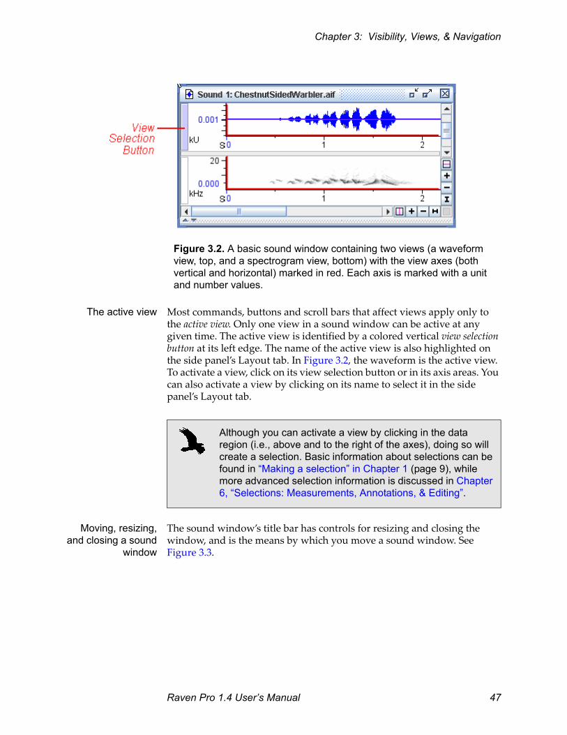
Figure 3.2 Sound Window
Figure 3.2. A basic sound window containing two views (a waveform view, top, and a spectrogram view, bottom) with the view axes (both vertical and horizontal) marked in red. Each axis is marked with a unit and number values.
The active view Most commands, buttons and scroll bars that affect views apply only to the active view. Only one view in a sound window can be active at any given time. The active view is identified by a colored vertical view selection button at its left edge. The name of the active view is also highlighted on the side panel’s Layout tab. In Figure 3.2, the waveform is the active view. To activate a view, click on its view selection button or in its axis areas. You can also activate a view by clicking on its name to select it in the side panel’s Layout tab.
Moving, resizing,and closing a sound
window
The sound window’s title bar has controls for resizing and closing the window, and is the means by which you move a sound window. See Figure 3.3.
Although you can activate a view by clicking in the data region (i.e., above and to the right of the axes), doing so will create a selection. Basic information about selections can be found in “Making a selection” in Chapter 1 (page 9), while more advanced selection information is discussed in Chapter 6, “Selections: Measurements, Annotations, & Editing”.
Raven Pro 1.4 User’s Manual 47
Chapter 3: Visibility, Views, & Navigation
Figure 3.3 Moving and Resizing a Sound Window
Figure 3.3. The title bar, with controls to resize and close a sound window. The title bar is also the anchor for moving the sound window.
To move the window around, simply click and drag on the title bar.
To minimize the window (to reduce the whole window to a short title bar at the bottom of the Raven window) click on the Minimize icon in the title bar. Clicking on a minimized window’s title bar expands it again.
Clicking on the maximize icon makes the window fill the entire Raven desktop. When the window is maximized, you’ll notice the Maximize button changes into a Restore button. Clicking this Restore icon restores the sound window to its previous size and position.
Clicking on the Close icon closes the window; if you close it, you’ll have to reopen the sound file again by choosing File > Open Sound Files..., by typing <Ctrl-O> (Windows, Linux) or <Command-O> (Mac OS), or by using the Recent Files section of the File menu.
You can also resize the window by clicking and dragging on an edge or any corner of the window. On Mac OS, you must drag from the bottom right corner to resize the window.
Scrollbars The horizontal and vertical scrollbars in a Raven sound window always refer to the active view. The length of the horizontal scrollbar in a waveform or spectrogram view corresponds to the total duration of the sound that is in Raven’s working memory.1 The length of a scrollbar’s scroll thumb (Figure 3.4) relative to the length of the entire scrollbar, indicates what proportion of the corresponding axis is visible in the view pane.
1. If you opened the entire sound at once (the default), the duration of the sound in memory is the duration of the entire sound file or file sequence. If you opened the sound in a paged window, the duration in memory is the length of one page. See “Configuring a new paged sound window” in Chapter 7 (page 188) for more on paged sound windows.
48 Raven Pro 1.4 User’s Manual
Chapter 3: Visibility, Views, & Navigation
Figure 3.4 Scrollbars
Figure 3.4. A sound window with its scrollbars and scroll thumbs labeled in red.
As touched on in “Filtered play” in Chapter 1 (page 9) the location of the scroll thumb within the scrollbar indicates the view’s position relative to the data. When the horizontal scroll thumb of a waveform or spectrogram is at the left edge of the scrollbar, the start of the data is aligned with the position marker (Figure 3.4).
Axis units in views The units used on the axes are indicated in the lower left corner of each view. In the waveform, the units are seconds (S) for the horizontal time axis, and kilounits (kU) for the vertical amplitude axis. In the spectrogram,
Raven displays a gray background for areas in each view pane that are beyond the limits of the data, for example before the beginning or after the end of a signal in the time dimension.
Raven Pro 1.4 User’s Manual 49
Chapter 3: Visibility, Views, & Navigation
the units are seconds (S) for the horizontal time axis, and kilohertz (kHz) for the vertical frequency axis.
Major and minorgrid lines
You can choose to overlay a grid onto any of the views in Raven by checking the corresponding box in the layout tab of the side panel. The spacing of the major and minor grid lines is determined by the spacing of the major and minor tickmarks on an axis. You can configure which grids appear in which views by right-clicking on a sound (or Control+clicking on a Mac) and choosing Configure Grids... from the contextual menu, or using View> Configure Grids....
Position markers Each view that Raven displays has a horizontal and a vertical position associated with it, shown by a magenta line, known as a position marker. You have already seen how the time position marker in a waveform view indicates the current time during scrolling play (“Filtered play” on page 9).
Notice that when you move the time position of either the waveform or spectrogram, the time position marker in the other view moves with it. This is because views that share a dimension (e.g., the time dimension for waveform and spectrogram views) are by default linked by their position in that dimension. More detailed information regarding linkage of views is discussed in “Linking and unlinking views” on page 62.
Centering a position You can move the horizontal or vertical position marker of a view relative to the window by grabbing it with the mouse and dragging it. To move a particular point in the data shown in a view to the horizontal or vertical center of the view pane, place the position marker on the point of interest, then click the corresponding Center Position button (Figure 3.5). The position marker and the underlying data will jump to the center of the
The “units” displayed on the vertical axis of a waveform view are the actual sample values in the signal, which are propor-tional to the sound pressure at the microphone when the sound was recorded.
When we speak of the “horizontal position marker” we mean the line that marks the horizontal position, which is a vertical line.
50 Raven Pro 1.4 User’s Manual
Chapter 3: Visibility, Views, & Navigation
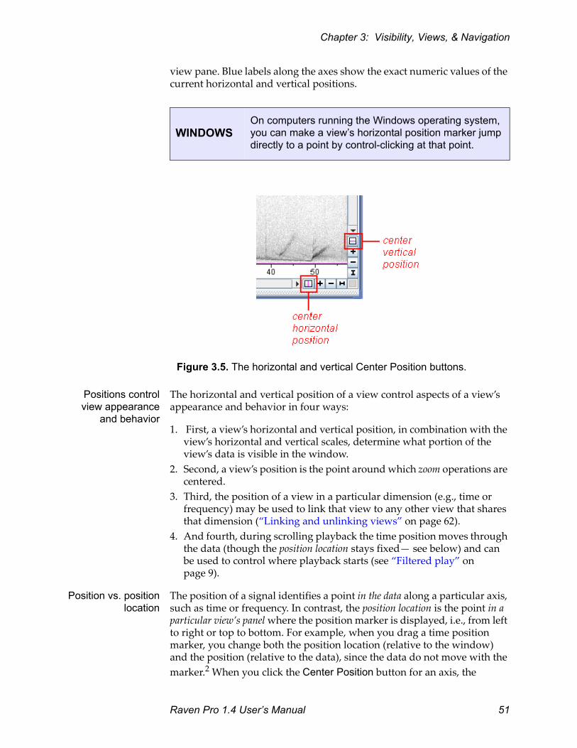
view pane. Blue labels along the axes show the exact numeric values of the current horizontal and vertical positions.
Figure 3.5. Center position buttons
Figure 3.5. The horizontal and vertical Center Position buttons.
Positions controlview appearance
and behavior
The horizontal and vertical position of a view control aspects of a view’s appearance and behavior in four ways:
1. First, a view’s horizontal and vertical position, in combination with the view’s horizontal and vertical scales, determine what portion of the view’s data is visible in the window.
2. Second, a view’s position is the point around which zoom operations are centered.
3. Third, the position of a view in a particular dimension (e.g., time or frequency) may be used to link that view to any other view that shares that dimension (“Linking and unlinking views” on page 62).
4. And fourth, during scrolling playback the time position moves through the data (though the position location stays fixed— see below) and can be used to control where playback starts (see “Filtered play” on page 9).
Position vs. positionlocation
The position of a signal identifies a point in the data along a particular axis, such as time or frequency. In contrast, the position location is the point in a particular view’s panel where the position marker is displayed, i.e., from left to right or top to bottom. For example, when you drag a time position marker, you change both the position location (relative to the window) and the position (relative to the data), since the data do not move with the marker.2 When you click the Center Position button for an axis, the
WINDOWSOn computers running the Windows operating system, you can make a view’s horizontal position marker jump directly to a point by control-clicking at that point.
Raven Pro 1.4 User’s Manual 51
Chapter 3: Visibility, Views, & Navigation
position marker jumps to the corresponding (horizontal or vertical) center of the view panel, and the data move with it— i.e., the position location changes, but the position (relative to the data) does not.
Figure 3.6. Centered pos markers w/gray bkgrd
Figure 3.6. Waveform and spectrogram views with centered position markers, positioned at the start of the signal (left edge of horizontal scrollbar) and the lowest frequency (bottom end of vertical scrollbar) of the spectrogram. The vertical scrollbar refers to the spectrogram view, because the spectrogram is the active view.
Scale of a view Each view that Raven displays has a horizontal and vertical scale associated with it. The scale determines the relationship between the dimensional units shown along that axis (e.g., seconds or kilohertz) of the view and display units (e.g., pixels, centimeters, or inches) on your computer screen. The scale at which the entire extent of an axis just fits in the view pane is called the default scale for that axis. When you first open a sound file, the time scale of the waveform view is set to the default. When you first create a spectrogram (information on creating views will be discussed later in the chapter) the frequency scale is set by default so that the entire frequency range of the signal fits vertically in the spectrogram pane.
Setting the scale ofview axes
The scale and position of the horizontal and vertical axes of any view can be changed using the zoom controls and scrollbars, as described in the next section. However, more precise control of scale and position is available in the Configure View Axes dialog box (Figure 3.7). To display the Configure View Axes dialog box, choose Configure View Axes... from the contextual menu for any view or from the View menu for the active
2. The one exception is when you try to drag the position marker beyond the lim-its of the signal. In that case, the end point of the signal will move with the marker, and you will be changing the position location but not the position (which is set to one of its limits already).
52 Raven Pro 1.4 User’s Manual
Chapter 3: Visibility, Views, & Navigation
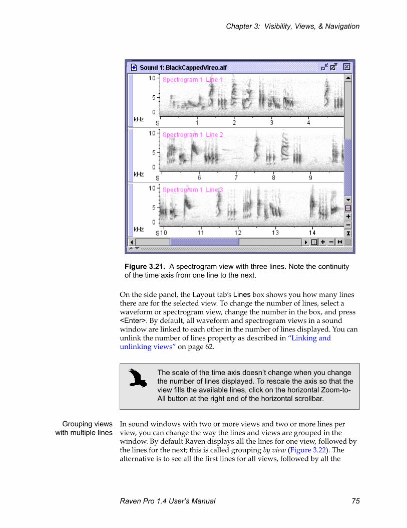
view. You can enter precise values for the position and scale of the view’s horizontal and vertical axes. Scale is specified in units per line of the view (see “Multiple-line views within sound windows” on page 74).
Figure 3.7 Changing time scale
Figure 3.7. The original file (top left) is shown with the default time scale. Below that (bottom left) is the sound with its time scale changed to 10 Seconds/Line. The Configure View Axes box is shown (right) with the edited time scale displayed. You can see the original view shows more than 20 seconds of the signal, while the bottom view (with the altered time scale) shows only 10 seconds of the signal across the line.
Changing viewscales by zooming
At the scale of magnification shown in Figure 3.6, you can’t see individual cycles of oscillation of the waveform view (top); what you see is the envelope of the entire signal. In order to see more detail of a signal, you must adjust the zoom level of the view. In the lower right-hand corner of a Raven sound window are the zoom controls for the active view (Figure 3.8). Buttons marked with ‘+’ and ‘-’ at the right and bottom ends of the horizontal and vertical scrollbars respectively increase and decrease magnification (zoom in and out) around the current position along that axis.
Raven Pro 1.4 User’s Manual 53
Chapter 3: Visibility, Views, & Navigation
Figure 3.8. Zoom buttons
Figure 3.8. The zoom controls, which apply to the active view. The Zoom to Selection button is gray if no selection exists in the signal.
Zoom details Each time you click a Zoom In or Zoom Out button, the corresponding axis of the active view is re-scaled by a factor of (= 1.41). Thus, clicking the Zoom In or Zoom Out button twice in succession changes the scale by a factor of 2. To zoom in horizontally on a view, first make sure that view is active, then move the horizontal position marker to the point where you want to center the zoom. Click the ‘+’ button at the end of the horizontal scrollbar, and observe how the display changes. Clicking the ‘-’ button reverses the change.
Each time that you zoom in or out horizontally or vertically, the corresponding scroll thumb shortens or lengthens to indicate what proportion of the signal is visible. (Remember that the scroll thumb is half the length of the scrollbar when that axis’s scale is set to its default value.)
Zooming inhorizontally
If you click the horizontal ‘+’ (zoom in) button repeatedly the scale will eventually be stretched to the point where Raven displays the individual samples in the waveform as dots (Figure 3.9).
2
54 Raven Pro 1.4 User’s Manual
Chapter 3: Visibility, Views, & Navigation
Figure 3.9 Zoom to Sample Points
Figure 3.9. A sound window with its waveform view (top) horizontally zoomed in enough to display individual sample points.
As mentioned before, the spectrogram and waveform views are linked by their time scale (and time positions.) So, you’ll notice that both the waveform and spectrogram views zoomed in, even though only one of them is the active view.
Zooming vertically To zoom vertically in the spectrogram, activate that view, and drag the vertical position marker to the point where you want to center the zoom. Click the ‘+’ or ‘-’ button at the bottom of the vertical axis to increase or decrease magnification around the vertical position marker.
Notice that changing the vertical position or scale of the spectrogram has no effect on the waveform. The vertical dimensions of the views are different (amplitude in the waveform, frequency in the spectrogram), so the vertical scales of the views cannot be linked.
Zoom to all To reset the horizontal or vertical scale of a view to display the entire axis, click on the corresponding Zoom To All button, marked with a horizontal or vertical I-beam icon (Figure 3.8, page 54).
Zoom to selection The Zoom To Selection button rescales the active view so that the active selection fills the view frame. If there is no active selection, the Zoom To Selection button is not available. In the spectrogram view, select a rectangular area to enlarge by clicking and dragging the mouse pointer. Then click on the Zoom To Selection button in the lower right corner of the sound window (Figure 3.8, page 54).
Raven Pro 1.4 User’s Manual 55
Chapter 3: Visibility, Views, & Navigation
View Types
The six main viewtypes
Waveform view
When you open a sound in Raven, the top view in a sound window is a waveform view by default. This view displays an oscillogram which is a graph of the sound showing amplitude versus time.
Spectrogram view
The second view shown by default in a sound window, below the waveform view, is a spectrogram view. It shows time on the horizontal axis, frequency on the vertical axis, and relative power at each point as a color (grayscale by default.)
Spectrogram Slice view
A spectrogram slice view is a plot of relative intensity versus frequency at a particular point in time within a signal. A spectrogram slice represents a vertical cross section through a spectrogram at a single time, but is rotated 90° so that the frequency axis is horizontal. In fact, a spectrogram is built of a series of spectrogram slices stacked side by side (with their frequency axes running vertically).
Where a spectrogram view shows a series of slices at successive points in time, and represents power at each frequency by a color value, a spectrogram slice view shows only one slice and represents power at each frequency on a line graph. The relationship between spectrogram and spectrogram slice views is explained in more depth in Chapter 5, “Spectrographic Analysis”.
Selection Spectrum view
These show the average spectrum of a sound over the time interval defined by a user-made active selection. More information about selections and how they affect this view type can be found in “Selection spectrum views” in Chapter 5 (page 139).
Beamogram View
Beamforming provides a means for determining a sound source's likely bearing relative to a multi-channel array of sensors. The beamogram view creates a plot of potential bearing angles versus time. Areas of higher energy in the beamogram view correspond to greater likelihood that specific angles represent actual sound source bearings. More information about determining source directions using the beamogram view can be found in “Bearing analysis: Beamforming, Beamogram View, and Max Bearing Measurement” in Chapter 8 (page 213).
56 Raven Pro 1.4 User’s Manual
Chapter 3: Visibility, Views, & Navigation
Beamogram Slice view
The beamogram slice view represents a vertical cross section of the beamogram view, showing the potential bearing angles at a specific point in time. Potential bearing angles are plotted on the horizontal axis, with vertical values corresponding to the likelihood that a sound is coming from the corresponding direction. More information regarding the beamogram slice view and its relation to the beamogram view can be found in “Bearing analysis: Beamforming, Beamogram View, and Max Bearing Measurement” in Chapter 8 (page 213).
Color Bar View
A color bar view serves as a key to the current spectrogram color scheme. It displays the spectrum of colors in the color scheme along with their associated intensity values. While this view contains no new information about the sound, it can be helpful for visually interpreting spectrograms.
Making a new view New views are created by using the appropriate buttons located on the view toolbar (Figure 3.10).
Figure 3.10 New view buttons on the control toolbar
Figure 3.10. The new view buttons on the view toolbar.
Open a sound file like ChestnutSidedWarbler.aif. The sound window shows a spectrogram and waveform view by default. To create a new view, like a spectrogram slice view, simply click on the New Spectrogram Slice button in the view toolbar. Alternately, you can choose View > New > Spectrogram Slice View..., or type <Ctrl-L> (Windows, Linux) or <Command-L> (Mac OS). The Configure New Spectrogram Slice View dialog box should appear (Figure 3.11.).
Raven Pro 1.4 User’s Manual 57
Chapter 3: Visibility, Views, & Navigation
am Slice View dialog box
Figure 3.11. The Configure New Spectrogram Slice View dialog box.
This dialog box lets you specify various parameters that affect the appearance of the spectrogram. For now, don’t worry about what these parameters mean; they are explained in detail in “Configuring spectrographic views” in Chapter 5 (page 112). Click OK to accept the default settings and compute the spectrogram slice view.
The sound window is re-drawn with an additional view pane, containing the new spectrogram slice view. If the time position marker of the waveform or spectrogram view is at the very beginning of the data (where Raven puts it by default when opening a new signal) the spectrogram slice view does not display any data (Figure 3.12).
58 Raven Pro 1.4 User’s Manual
Chapter 3: Visibility, Views, & Navigation
Figure 3.12 New Spectrogram Slice View
Figure 3.12. This sound window contains the usual waveform and spectrogram views, but it also contains a blank spectrogram slice view as well. The spectrogram slice view displays no data when the time position marker of the spectrogram and waveform view is located at the start of the data (all the way to the left).
Showing data in anew view
To see valid data, drag the time position marker to the right in either the waveform or spectrogram view (Figure 3.13). (For a complete explanation of why no data are visible in the spectrogram slice view when the position marker is at the start of the signal, see Chapter 5, “Spectrographic Analysis”.)
Raven Pro 1.4 User’s Manual 59
Chapter 3: Visibility, Views, & Navigation
Figure 3.13 Spectrogram Slice view with data
Figure 3.13. The same sound window as shown in Figure 3.12 but with the time position marker (the vertical magenta line) moved to a position in the waveform and spectrogram data. The spectrogram slice view now displays the data from the time designated by the time position marker.
Selected viewdictates toolbar
content
Remember that the active view in a sound window is marked by the highlighted view selection button to the left of the view (for example, the spectrogram view is active in Figure 3.13). The activated contents of the toolbars are dictated by which view is active in the current sound window. For example, if a spectrogram view is active, the brightness and contrast sliders in the spectrogram toolbar become active (Figure 2.12 on page 37). If any of the other views are active, the brightness and contrast sliders are grayed out because they have no relevance in those cases.
The zoom window The zoom window is a separate window on the Raven desktop that can be used to view selections from any open sound. Once a zoom window is opened, it displays a magnified view of the active selection of the active sound. If the zoom window is the active window, it will display the active selection from the previously active sound. The zoom window automatically updates as you move through selections in a sound, making it particularly useful for browsing details of selections without having to manually zoom in on each one before advancing.
To open a zoom window, choose Zoom Window from the Window menu. You can configure the views or change display settings in the zoom window through the context menu or side panel in the same way as other sound windows. These settings are applied specifically to the zoom window, and override the display settings of the original sound when displaying selections. For multi-channel files the zoom window only
60 Raven Pro 1.4 User’s Manual
Chapter 3: Visibility, Views, & Navigation
displays the channels containing the active selection; however, you can choose to add other channels from the side panel. Figure 3.14 shows the default zoom window with the parent sound window for a selection.
Figure 3.14Zoom Window
Figure 3.14. The zoom window displays a magnified view of the active selection, showing only those channels that contain the selection.
When the zoom window is active the cursor will change from its current setting to a play cursor, allowing you to play the selection simply by clicking in the zoom window. This is the case for both the create selection and activate selection modes. However, the Grab and Scroll mode retains its normal function in the zoom window.
When a workspace is saved, the zoom window’s visibility and settings will be saved as well. However, if the zoom window is active when the workspace is saved, its contents may not be fully restored. If another sound window is active, however, the zoom window will restore accordingly.
Raven Pro 1.4 User’s Manual 61
Chapter 3: Visibility, Views, & Navigation
Linking and unlinking views
Two views that share a dimension— such as time or frequency— can have their positions and scales either linked or unlinked by that dimension. When the positions of two views are linked, moving the position of either one (by moving the corresponding scroll thumb, or by moving the position marker within the window) causes the positions of both views to move together. When the scales of two views are linked, changing the scale of either one (using the zoom buttons) causes both views to be re-scaled. In the examples you’ve seen so far, waveform and spectrogram views have been linked by time position and in time scale.
When you open or record a signal and create multiple views, each view is initially linked in position and scale to every other view that shares its dimensions. For example, waveforms and spectrograms are initially all linked to each other in time position and time scale, and spectrogram and spectrogram slice views are linked in frequency position and frequency scale. Spectrograms and waveforms cannot be linked in frequency because waveforms have no frequency dimension.
Unlinked views In some situations, it can be useful to work with views that are unlinked from each other in particular ways. For example, Figure 3.15 shows two spectrogram views of a signal that is 53 seconds long. The views are linked in time position but unlinked in time scale. Unlinking the time scales makes it possible to view simultaneously an eight-second portion segment of the signal (upper view), and a close-up of a two-second segment contained within it (lower view). Since the two views remain linked in time position, the position markers provide a reference point to show where the close-up view is located within the entire signal. As either view is scrolled horizontally through the signal, the linked position markers identify the same point in time in both views.
62 Raven Pro 1.4 User’s Manual
Chapter 3: Visibility, Views, & Navigation
Figure 3.15. Two linked spgs, diff time scales
Figure 3.15. Two spectrogram views of the file “BlackCappedVireo.aif” that are linked in time position, but unlinked in time scale. The upper spectrogram shows 7.8 seconds of the signal; the lower spectrogram is a close-up of 2.0 seconds. The highlighted rectangle identifies the same selection in both views. The time position markers in both spectrograms identify the same time, because the time positions are linked.
Unlinking viewsthrough the
contextual menu
To create two spectrograms that are unlinked in time scale as discussed in the above example (Figure 3.15):1. Open a signal.2. Make a second spectrogram by clicking the New Spectrogram button
(Figure 3.10, page 57), or typing <Ctrl-G> (Windows, Linux) or <Command-G> (Mac OS).
Place the mouse pointer on the second spectrogram, activate the contextual menu, and choose Unlink View > Time Scale.
Now try using the zoom buttons to change the time scale of the first spectrogram. Notice that the time scales of the waveform and the first spectrogram change together, but the time scale of the second spectrogram does not change. If you activate the second spectrogram, and zoom in time, its time scale changes, while the time scales of the waveform and the first spectrogram remain unchanged. If you scroll any of the three views, their position markers will move in synchrony, because all three are still linked by time position.
Raven Pro 1.4 User’s Manual 63
Chapter 3: Visibility, Views, & Navigation
Restoring orcreating new
linkages throughthe linkage tab
To restore linkages between views that have been unlinked, or to create linkages between views that have never been linked, activate the Linkage tab in the Raven side panel. (If the side panel is not visible, click on the right-pointing triangle at the top (Windows, Linux) or bottom (Mac OS) of the separator bar at the left edge of the Raven window.)
At the top of the Linkage tab, there is a drop-down menu showing all of the linkable properties of the current views. Click on this menu, and choose Time Scale. If you created two spectrograms and unlinked them as described above, the tab will display three folder icons representing linkage groups, with names like “Group 1”, “Signal 1 Default”, and “New” (Figure 3.16). (The second group may be called “Signal 2 default”, “Signal 3 default”, etc., depending on how many signals you’ve opened in the current Raven session. If more than one signal is open, you will see a default linkage group for each signal.)
Figure 3.16 . Linkage tab.
Figure 3.16. The Linkage tab, showing the linkage groups for the Time Scale property corresponding to Figure 3.15
A linkage group is a set of views that are linked to each other by a particular property (in this case, Time Scale). Views that are in different linkage groups are unlinked from each other in that property.
Open the first two folders by double-clicking on them (or single-clicking the icon to the left of each folder icon). In the present case, the linkage group called “Sound 1 Default” contains the views called “Sound 1 Waveform 1” and “Sound 1 Spectrogram 1”; Group 1 contains “Sound 1 Spectrogram 2”. The active view is highlighted, and you can activate a different view by clicking on its name.
To link two views that are presently unlinked, drag the icon for one of the views to the linkage group that contains the other. In the case shown in Figure 3.16, you can unlink the waveform from Spectrogram 1 and link it
64 Raven Pro 1.4 User’s Manual
Chapter 3: Visibility, Views, & Navigation
to Spectrogram 2 by dragging its icon from the Default folder to the Group 1 folder.
When you move a view from one linkage group to another, the view is immediately redrawn if necessary so that its image has the correct scale, position, or other linkable property. If a linkage group contains only a single view, and you drag that view to a different linkage group, the original (now empty) group disappears.
Creating a newlinkage group
To create a new linkage group select one of the views listed by clicking on it, and drag it onto the folder labeled “New”. A new linkage group will appear in the list, containing the view that you moved.
Creating new linkedviews
To create a new spectrogram, spectrogram slice, or selection spectrum view that is linked by spectrogram parameters to an existing spectrographic view, choose New > Similar Spectrogram View, New > Similar Spectrogram Slice View, or New > Similar Selection Spectrum View from the contextual menu for any spectrographic view, or from the View menu for the active spectrographic view.
Other linkableproperties
In addition to its position and scale for each of its dimensions, every view has four other properties by which it can be linked to other views:•Position Location: Moving the location of the time or frequency position
bar in a view will also move the corresponding position bar in other views that are linked by Position Location.
•Color Scheme: Color schemes include color specifications for most of the graphical elements shown in a view (e.g., axes, backgrounds, selection boundaries), as discussed later in this chapter. Adjusting brightness and contrast settings for a spectrogram adjusts the settings for all spectrograms linked to it by Color Scheme. By default all views of a signal are linked to each other by Color Scheme.
•Channel Visibilities: In multi-channel signals (see Chapter 8, “Multi-channel Sounds”), hiding or showing particular channels of a view will also hide or show those channels in other views that are linked by Channel Visibility.
•Number of Lines: Changing the number of lines displayed for a view (see “Multiple-line views within sound windows” on page 74) automatically changes the number of lines displayed for any other views that are linked by Number of Lines. By default, all views in a signal that display a time axis are linked to each other by Number of Lines.
Additionally, spectrogram, spectrogram slice, and selection spectrum views can be linked by spectrogram parameters. If two views are linked
Raven Pro 1.4 User’s Manual 65
Chapter 3: Visibility, Views, & Navigation
by spectrogram parameters, then changing the parameters for either view automatically changes both views.
Linkage betweenspectrogram and
spectrogram sliceviews
When you request a spectrogram slice view, Raven actually calculates an entire spectrogram of the signal, but only displays one slice at a time. A spectrogram slice view thus has a “hidden” time axis. Which slice of the underlying spectrogram is displayed is determined by the view’s time position. By default, the time position of a spectrogram slice view is linked to the time positions of waveform and spectrogram views. As you move the time position marker of a spectrogram view, any spectrogram slice view that is linked to it is continually updated to show the cross-section of the spectrogram at the time position marker.
By default, new spectrogram and spectrogram slice views are also linked to each other by frequency position and frequency scale. When you move the frequency position of a spectrogram, the frequency position of any linked spectrogram slice views move as well, and vice versa. Similarly, when you zoom the frequency scale of any spectrogram slice view, the frequency scale of any linked spectrogram zooms as well. It is important to remember that the frequency scales of spectrogram and spectrogram slice views are rotated 90° from each other.
Controlling how views are displayed
Using tools and commands in the side panel’s Layout tab and in the View menu, you can rearrange the order of views and hide or show the non-data components of views such as the axes and position markers.
Another way to hide a view is to activate that view and choose Hide View from the View menu, or from that view’s contextual menu.
Deleting a view To delete a view, activate the view and choose Delete View from its contextual menu or from the View menu. When you delete a view (as opposed to hiding it), the memory occupied by that view is released for reuse. Re-displaying a hidden view occurs instantly, whereas re-
Views that share a linkable property can be linked even if they are in different signal widows. This can be useful for example in setting views of different signals to the same scale.
Even though a spectrogram slice view has a time position, it does not have a time scale, since the time axis of the underly-ing spectrogram is not displayed.
66 Raven Pro 1.4 User’s Manual
Chapter 3: Visibility, Views, & Navigation
displaying a view that was deleted requires that it be recalculated, which may take a significant amount of time.
Changing the orderin which views are
displayed
To rearrange the order in which views are displayed in the sound window, you can drag and drop view names in the Layout tab.
You can also move a view up or down within the sound window by choosing Move View Up or Move View Down from the View menu or the view’s contextual menu.
Hiding and showingwindow
components
The bottom pane of the side panel’s Layout tab contains a list of window components that can either be displayed or hidden. You can display or hide each component of the active window by checking or unchecking its checkbox. Figure 3.17. shows a sound window containing two views, with all components hidden.
Figure 3.17.. All components hidden.
Figure 3.17. A sound window with all components hidden.
By default, all window components are displayed except for line titles, which identify the view type and number of each view (Figure 3.18.). If the sound has multiple channels (see Chapter 8, “Multi-channel Sounds”) or a view has multiple lines, channel and line numbers are displayed in line titles as well.
When you activate a contextual menu in a view pane, view-specific commands in the menu apply to whichever view the mouse pointer is on when the menu is activated, irrespective of whether or not that view is active.
Raven Pro 1.4 User’s Manual 67
Chapter 3: Visibility, Views, & Navigation
Figure 3.18. . View titles.
Figure 3.18. A sound window showing a waveform and a spectrogram view, with line titles displayed.
Changing the Appearance of a Sound Window
Spectrogrambrightness and
contrast
When a spectrogram view is active, the brightness and contrast controls on Raven’s spectrogram toolbar become active too (Figure 2.12 on page 37).
If your spectrogram looks too dark or light, or if it’s hard to pick the signal out of the background, move the brightness and contrast sliders to achieve the desired appearance of the spectrogram. The brightness control adjusts the overall darkness of the spectrogram: for a grayscale spectrogram (the default), sliding the control to the right lightens the display.
The contrast control adjusts the number of different color (by default, grayscale) values that are shown in the spectrogram. In a grayscale spectrogram, moving the contrast slider all the way to the right makes the display black and white: all values below some threshold are assigned to white and the rest become black. In this case, the threshold between black and white is determined by the brightness control. With the contrast control all the way to the left Raven displays up to 200 shades of gray.
The box next to each control tells you what percent contrast or brightness you’ve set. If you prefer, you can type a percentage number into a box instead of moving the slider.
In addition to the toolbar controls, you can also configure spectrogram brightness and contrast by choosing Configure Brightness and Contrast... from a view’s contextual menu. In addition to a set of brightness and
68 Raven Pro 1.4 User’s Manual
Chapter 3: Visibility, Views, & Navigation
contrast sliders, the resulting dialog allows you to alter these parameters by specifying floor and ceiling values for the spectrogram and displays a plot illustrating how colors are assigned to each value in a spectrogram. The floor and ceiling threshold parameters determine the power levels beyond which all values are assigned the same color. In the case of a grayscale spectrogram, values below the floor threshold are all displayed as white, and values above the ceiling threshold are all displayed as black. For more information on the relationship between these threshold parameters and corresponding brightness and contrast values, see “Brightness and contrast” in Chapter 5 (page 130).
Figure 3.19Brightness and Contrast Dialog
Figure 3.19. The configure Brightness and Contrast dialog
Color schemes ofsound windows
Each view in a sound window has a particular color scheme. A color scheme consists of a spectrogram colormap and particular colors for items such as plottable measurements, active and inactive selection borders and fills, and the waveform line.
Raven Pro 1.4 User’s Manual 69
Chapter 3: Visibility, Views, & Navigation
A spectrogram colormap defines the relationship between power values in the spectrogram and colors used to display them. Raven provides six predefined colormaps: Grayscale, Hot, Cool, Standard Gamma II3, Bone, and Copper (Figure 3.20.). You can also create customized colormaps as text files as described in “Creating customized colormaps” in Chapter 11 (page 296). To change the colormap of a spectrogram, choose Color Scheme > Colormap-name from the spectrogram’s context menu, or from the View menu when the spectrogram is active. You can reverse the spectrogram colormap by choosing Color Scheme > Reverse Color Map from the spectrogram’s context menu, or from the View menu when the spectrogram is active. To display the spectrum of colors in the color map along with their associated intensity levels, you can add a color bar view to the sound window by clicking on the icon in the view toolbar or through the View > New menu.
3. The Standard Gamma II color map is included in Raven courtesy of Research Systems, Inc., a Kodak Company.
Views in a sound window are by default linked to each other by color scheme. If you change the colormap or any other item in a view’s color scheme, the affected colors will also change in any other views that are linked to it by color scheme.
70 Raven Pro 1.4 User’s Manual
Chapter 3: Visibility, Views, & Navigation
Figure 3.20.. Colormap examples
Figure 3.20. Four spectrogram views of the signal “CassinsKingbird.wav”, using four different, predefined colormaps. (a) Hot. (b) Standard Gamma II. (c) Bone. (d) Copper.
You can reverse the spectrogram colormap by choosing Color Scheme > Reverse Color Map from the spectrogram’s context menu, or from the View menu when the spectrogram is active.
Editing colorschemes
In addition to selecting spectrogram colormaps, you can also edit a view’s color scheme by choosing Color Scheme > Edit... from the view’s context menu, or from the View menu when the view is active. More information on customizing color schemes can be found in “Editing color schemes” in Chapter 11 (page 289).
Sound WindowPresets
You can save information about the layout of a sound window in a window preset, which you can later apply to another sound window (or to the same
In general, if the background of a spectrogram is white, then light colors represent low power. If the background is black, the dark colors of a colormap represent the low power.
Raven Pro 1.4 User’s Manual 71
Chapter 3: Visibility, Views, & Navigation
window). A window preset includes information about the size of a window, what views are displayed, whether or not the selection table is showing, and other properties (Table 3.1).
72 Raven Pro 1.4 User’s Manual
Chapter 3: Visibility, Views, & Navigation
To save a window preset, first configure the properties listed in Table 3.1 the way you want to save them, then choose View > Window Preset > Save As... . When the Save Sound Window Preset dialog box appears, enter a name for the preset, and click OK.
To apply a window preset that’s already been saved to the active sound window, choose View > Window Preset > Preset-name. When you apply a saved preset, the active window is redrawn with the properties specified in the preset, and any additional views are calculated as needed. If any of the open selection tables contain annotation columns, Raven will display a dialog where you can choose to keep, replace, or merge these columns with those in the preset.
Table 3.1. Window properties saved in window presets.
window size
view types, parameters, color schemes, positions, scales, sizes
spectrogram parameters
spectrogram brightness and contrast
selection table visibility and size
measurement list and annotation columns
selection label configuration
selection label visibility
axis visibility
major and minor grid visibility
line title visibility
position marker visibility
view selection button visibility
scrollbar visibility
Window presets must be saved in the folder Presets/Sound Window/ within the Raven program folder. You can also create additional folders within the Sound Window folder by clicking on the New Folder icon within the Save Sound Window dialog. These folders will appear as sub-menus in the Window Preset menu, with each submenu list-ing the presets in the corresponding folder.
Raven Pro 1.4 User’s Manual 73
Chapter 3: Visibility, Views, & Navigation
You can specify a window preset to apply when you first open a sound file in the Configure New Sound Window dialog box (Figure 1.3, page 4). You can change the name of the default window preset by editing the Raven preferences file, as described in “About Raven preferences” in Chapter 11 (page 299).
If you make changes to the properties of a window to which you’ve applied a preset, you can save the changes to the current preset by choosing View > Window Preset > Save “Preset-name”.
Multiple-line viewswithin sound
windows
Raven can display views that have a time axis (i.e., waveforms and spectrograms) across multiple lines (Figure 3.21). The values shown on the time axis of a multiline view start at the left end of the top line, go to the right end of that line and continue on from left to right on subsequent lines, like lines of text on a page.
Window presets take precedence over other presets that affect the appearance of the contents of a window. Thus, if you apply a window preset, spectrogram parameters, the measurement list, and the color scheme are all set as defined in the specified window preset, even if they were previously set to different values by choosing spectrogram, measure-ment, or color scheme presets.
74 Raven Pro 1.4 User’s Manual
Chapter 3: Visibility, Views, & Navigation
Figure 3.21. Multi-line spg.
Figure 3.21. A spectrogram view with three lines. Note the continuity of the time axis from one line to the next.
On the side panel, the Layout tab’s Lines box shows you how many lines there are for the selected view. To change the number of lines, select a waveform or spectrogram view, change the number in the box, and press <Enter>. By default, all waveform and spectrogram views in a sound window are linked to each other in the number of lines displayed. You can unlink the number of lines property as described in “Linking and unlinking views” on page 62.
Grouping viewswith multiple lines
In sound windows with two or more views and two or more lines per view, you can change the way the lines and views are grouped in the window. By default Raven displays all the lines for one view, followed by the lines for the next; this is called grouping by view (Figure 3.22). The alternative is to see all the first lines for all views, followed by all the
The scale of the time axis doesn’t change when you change the number of lines displayed. To rescale the axis so that the view fills the available lines, click on the horizontal Zoom-to-All button at the right end of the horizontal scrollbar.
Raven Pro 1.4 User’s Manual 75
Chapter 3: Visibility, Views, & Navigation
second lines for all views, and so on; this is called grouping by time (Figure 3.23).
Figure 3.22. VL grouping.
Figure 3.22. A sound window containing two views, each with two lines, grouped by view. All lines of the waveform view are in the top group, all lines of the spectrogram view are in the next group.
76 Raven Pro 1.4 User’s Manual
Chapter 3: Visibility, Views, & Navigation
Figure 3.23. LV grouping.
Figure 3.23. The same two views shown in Figure 3.22, but grouped by time. The first lines of both views are in the top group; the second lines of both views are in the next group.
To change the grouping, choose View or Time from the pull-down menu labeled “Group By”, in the side panel’s Layout tab.
Working with morethan one sound
Raven lets you work with more than one sound at a time. When more than one sound window is open, the tools in Raven’s toolbar (e.g., New View buttons, brightness, contrast, and playback controls) and in the side panel’s Layout and Playback tabs always refer to the active window (the one window in which the title bar is colored). The side panel’s Linkage tab shows views for all sounds that are open, since Raven lets you link views of different sound windows to each other. You can activate a sound window by clicking anywhere in it with the mouse. You can also activate a
The horizontal separator bar that Raven displays between top-level groupings (i.e., between views in View grouping or between lines in Time grouping) is wider than the bar used between second-level groups.
Raven Pro 1.4 User’s Manual 77
Chapter 3: Visibility, Views, & Navigation
window by choosing its name from the Window menu, or by clicking on the name of one of its views in the side panel’s Linkage tab.
Tile/Cascadewindows
When you have multiple sound windows open, Raven can arrange them neatly for you on the desktop. If you choose Window > Tile Windows, Raven resizes and repositions all of the windows so that they are all the same size and fill the desktop (as nearly as possible) without overlapping each other. Choosing Window > Tile Windows Horizontally arranges the windows in a row such that they are all the same width and fill the desktop. Similarly, choosing Window > Tile Windows Vertically arranges the windows in a column such that they are all the same height and fill the width of the desktop. See Figure 3.24 for examples of these tiling options.
If you choose Window > Cascade Windows, Raven resizes and repositions all of the windows so that they are all the same size and as large as possible, overlapping so that their title bars are all visible (Figure 3.25).
78 Raven Pro 1.4 User’s Manual
Chapter 3: Visibility, Views, & Navigation
Figure 3.24 Tile Windows
Figure 3.24. Examples of tiled sound windows (a) 2 to 3 sounds will be tiled in one column (b) 4 to 8 sounds will be tiled in two columns and (c) 9 to 12 sounds will be tiled in three columns. (d) 4 windows tiled horizontally. (e) 4 windows tiled vertically
Raven Pro 1.4 User’s Manual 79
Chapter 3: Visibility, Views, & Navigation
Figure 3.25 Cascade Windows
Figure 3.25. An example of cascaded sound windows. Here, the windows are stacked on each other with all title bars visible.
Apply currentwindow layout to all
windows
To apply all of the active window’s layout to all currently open windows, choose View > Apply To All. Window layout includes all of the information that would be stored in a sound window preset, including window size, view visibility and scale, spectrogram parameters, and spectrogram brightness and contrast. A complete list of window properties affected by the Apply To All command is given in Table 3.1.
80 Raven Pro 1.4 User’s Manual
Chapter 4 Signal Acquisition (Recording)
About this chapter
This chapter describes how to acquire (digitize) signals with Raven, and assumes that you are familiar with basic Raven concepts and operations as described in earlier chapters.
In order to make good recordings with Raven, you should be acquainted with the basic concepts of digital sound representation discussed in Appendix A, “Digital Representation of Sound”. Failure to understand concepts such as sample rate and sample size can lead to digitized signals that are poor in quality or distorted in various ways.
In this chapter you’ll learn how to:•choose whether to record to memory, to a file, or to a file sequence•create and configure a recorder window•create and work with real-time signal views in a recorder window
Overview of signal acquisition
Raven acquires (records) audio signals via recorders. A recorder is represented on the Raven desktop by a recorder window that can display one or more views of a signal in real time as the signal is being acquired. A recorder window is like any other Raven sound window, except that it has additional controls for starting and stopping recording and cannot be edited.
Recording modes Raven provides three different recording modes, which differ in where the signal is stored as it’s recorded.•Record to memory: When recording to memory, audio data are not
automatically saved to disk files, but reside only in a portion of Raven’s temporary memory allocated as a recording buffer. You can specify the size of the buffer (in seconds) when you configure a recorder. During recording, audio data are stored in the buffer until the buffer is full, and then the oldest data are continually discarded to make room for new data being acquired. For example, if the buffer size is 30 seconds (the default), the buffer will always contain the most recent 30 seconds of data during recording; data recorded more than 30 seconds ago are lost. While a signal is in the recording buffer, you can manually save it to a disk file, or save selections from it. Recording to memory is useful for exploratory browsing through recordings when you don’t need to save
Raven Pro 1.4 User’s Manual 81
Chapter 4: Signal Acquisition (Recording)
the data to files, or when the signals you’re interested in saving are sparsely distributed among sections that you don’t want to save.
•Record to file: When recording to a single file, Raven saves audio data directly to a disk file for a specified amount of time, then stops. You can also manually stop recording to disk before the specified time has finished.
•Record to file sequence: When recording to a file sequence, Raven saves audio data continuously to a series of files, each of which is a specified size. Successive files in a sequence are named according to a template that you specify, which can incorporate a sequence number or a timestamp. Raven also saves a list file, which can be used to open the file sequence as a single continuous signal.
Creating a recorder You create a recorder by specifying a set of configuration parameters in the Configure New Recorder dialog box (Figure 4.1), which is invoked by clicking on the Record button on the Raven toolbar (identified by the microphone icon, left) or by choosing File > New Recorder....
Figure 4.1. New Recorder dialog.
Figure 4.1. The Input tab of the Configure New Recorder dialog box.
You use the Record To drop-down list in this dialog to choose whether to record to Memory, a File, or a File Sequence. Depending on which recording destination you choose, different tabs appear in the dialog box. The following sections discuss the configuration options on each tab.
Recording Input
The Input tab (Figure 4.1) allows you to choose and configure an audio input device. The Input tab is displayed for all three recording modes.
82 Raven Pro 1.4 User’s Manual
Chapter 4: Signal Acquisition (Recording)
Device Click on the Device drop-down list to see a list of all available audio input devices. By default, the operating system’s default audio input device is selected. The name that is shown for this device will be the name of the default audio input device (typically a built-in sound card) for your computer. The audio input device obtains its input from a recording source that you choose using controls supplied by your computer’s operating system. Appendix C, “Configuring Audio Input” explains how to configure your operating system’s controls to choose a recording source (e.g., the computer’s built-in CD player, a microphone, or line input jack) for audio input.
Each audio input device is characterized by a set of available sample rates at which signals can be recorded, the number of channels that can be recorded, and a set of sample formats. Each of these parameters is discussed below. Some devices may also have additional parameters that can be configured.
Sample Rate The Sample Rate drop-down list displays all of the sample rates available for the selected input device. Typically, the sample rates available are determined by the underlying sound input hardware. The Sample Rate parameter specifies the rate at which an analog electrical signal representing a sound is sampled to create the digital signal. Be sure to choose a sample rate that is at least twice as high as the highest frequency in the recording you want to acquire, in order to avoid signal distortion due to aliasing. See Appendix A, “Digital Representation of Sound” for a discussion of aliasing and the trade-offs involved in choice of sample rate.
Channels The default audio input device on most computers provides for one- (mono) or two-channel (stereo) acquisition. For signals that are acquired in stereo, the Left and Right channels are identified within Raven as Channel 1 and 2, respectively. To acquire only one channel, uncheck either the Left or Right checkbox. The remaining channel will be acquired as Channel 1.
If you selected a device that supports input of more than two channels, each channel is represented by a numbered checkbox. If you disable input of some channels, data from the channels that are recorded will be represented in the resulting acquired signal in channel-number order, and renumbered sequentially beginning at Channel 1. For example, if you are recording from a 16-channel input device, and you select only input channels 1, 5, 7, and 12, then data from these channels will be represented in channels 1, 2, 3, and 4 respectively of the acquired signal.
Raven now includes support for multi-channel recording using both NI-DAQ and ASIO audio input devices. For more information about using this feature, please see Appendix C, “Configuring Audio Input”.
Raven Pro 1.4 User’s Manual 83
Chapter 4: Signal Acquisition (Recording)
Sample Format The Sample Format drop-down list shows all of the sample formats available for the selected virtual recording device. The default input device on most computers supports two formats, 8-bit and 16-bit signed PCM (Pulse Code Modulation). Some sound cards will support 24-bit signed PCM. A larger sample size (more bits) results in a better quality digitized signal (higher signal-to-noise ratio), but may also increase the storage requirements for signals saved to disk files. See Appendix A, “Digital Representation of Sound” for a discussion of the trade-offs involved in choice of sample size.
Raven always represents signals internally with 32-bit floating point samples. As a result, Raven accurately stores signals recorded with signal sizes up to 24 bits. If you choose an input sample size greater than 24 bits, the input values may be truncated, resulting in a distorted signal. (for more on floating point values and truncation, see the footnote under “Sample Size” on page 87).
Recording Display
The Display tab (Figure 4.2) allows you to configure the recorder window, and is displayed for all three recording modes.
Figure 4.2 . Recorder Display tab.
Figure 4.2. The Display tab of the Configure New Recorder dialog box.
Buffer Size The buffer size determines how much of the signal is retained in memory and can be visible in the recorder window during signal acquisition. You
84 Raven Pro 1.4 User’s Manual
Chapter 4: Signal Acquisition (Recording)
can specify buffer size either in seconds or minutes. You can use the drop-down list to choose time units of seconds or minutes. The default buffer size is 30 seconds.
During recording, audio data remain in memory for the duration of the buffer, and are then discarded to make room for new incoming data. If you’re recording to memory, data that are discarded from the buffer are lost permanently. When recording to a file or a file sequence, data that are gone from the buffer can be retrieved by opening the file(s) that were saved during the acquisition.
Update Rate The update rate determines how many times per second views in the recorder window are redrawn during signal acquisition. The default rate is 10 Hz. There is a trade-off between the perceived smoothness of the scrolling real-time display and Raven’s responsiveness to user interaction. If the update rate is too low, scrolling views move in visibly discrete steps, resulting in a jittery display. If the update rate is too high, Raven will be slow to respond to user actions such as mouse clicks or keyboard commands. In practice, the best rate will depend on the size of the recorder window, the number and type of views it contains, and the speed of the computer. The default update rate of 10 Hz provides a good balance between display smoothness and performance on most computers. You may need to experiment to determine what update rate provides the best performance on your computer. See “Reconfiguring an existing recorder” on page 98 to learn how to change the update rate once a recorder is running.
Latency The Latency value on the Display tab specifies the difference, for a running recorder, between the current time and the active view’s time axis position (by default, the right-hand edge of the window). Specifying a display latency greater than zero introduces a delay in the display of data in real-time views.
By specifying a display latency greater than zero, you give Raven some additional time to compute a view and build the corresponding image before it needs to be displayed. A small display latency (e.g., 0.1 or 0.2 seconds) often eliminates the flickering grey band that is sometimes visible at the right-hand edge of some real-time views, while only resulting in a barely-perceptible delay in the display of real-time data. Non-zero display latencies also result in smoother updates to real-time spectrogram slice views.
Display latency vs. processing latency
When a recorder is running, you may observe a flickering gray band at the right-hand edge of some real-time views. This band is more evident in recorder windows that are displayed at large sizes or that contain many views, when the time axis is zoomed in, and on slower computers. This band represents the view’s processing latency, which is the difference between the current time (by default the right-hand edge of the window) and the last time for which Raven has displayed data in the view. The
Raven Pro 1.4 User’s Manual 85
Chapter 4: Signal Acquisition (Recording)
processing latency is always greater than zero because it takes some time for Raven to build the visual image of the data to be displayed in the view. Real-time views scroll at a fixed rate, irrespective of the rate at which Raven builds images for display. When a view scrolls and no new image data are available for display, Raven draws a gray band to fill in the time interval for which the image is not yet available. As soon as the image is computed, it replaces the gray band. Processing latency is typically longer for spectrogram or spectrogram slice views than for waveforms, because spectrograms require more calculation than waveforms. The processing latency (hence the width of the gray band) varies from moment to moment for each view as Raven rapidly switches among the various tasks involved in updating the views in the recorder window. When the processing latency is small relative to the time scale shown in a view, the flickering gray band disappears. When it is larger, the band becomes more prominent.
Window preset The Window Preset drop-down list on the Display tab shows the name of the window preset that will be applied to the recorder window when it is first created. Window presets define what views are visible in a window, as well as window size, selection mode, and other properties. You can choose from all of the window presets that are currently defined by clicking on the drop-down menu icon to the right of the Window Preset field. Window presets are discussed further in “Sound Window Presets” in Chapter 3 (page 71).
File Format
The File Format tab appears only if you choose Record to File or Record to File Sequence.
86 Raven Pro 1.4 User’s Manual
Chapter 4: Signal Acquisition (Recording)
Figure 4.3. File Format tab.
Figure 4.3. The File Format tab of the Configure New Recorder dialog box.
File Format Raven can acquire audio data directly to files saved either in AIFF (Audio Interchange File Format, filename extension .aif) or in WAVE format (filename extension .wav). WAVE files can be opened by most other programs that work with audio data. AIFF files can be opened by most Macintosh programs that work with audio data, and some programs on other platforms. Raven can open either type of file.
Sample Size The Sample Size parameter specifies the “bit depth” of the samples saved in the file(s) created during signal acquisition. Raven always represents signals internally with 32-bit floating point samples. Therefore, values recorded using an input sample size greater than 24 bits may be truncated, resulting in distorted signal.1See Appendix A, “Digital Representation of Sound” for a discussion of the trade-offs involved in choice of sample size.
1. In general, individual samples in a signal of sample size n can have 2n possible values, from -2n-1 to 2n-1-1. Thus, in general a 32-bit representation has 4,294,967,296 (=232) possible sample values, from -2,147,483,648 to +2,147,483,648. However, by using a floating point representation, Raven stores each value as a combination of a 24 bit integer and an 8 bit exponent. This allows values across a much greater range to be stored, but limits the pre-cision to which larger values can be represented. As such, signals recorded using an input sample size greater than 24 bits will be truncated to include only 24 bits of precision, resulting in increased distortion for large values.
Raven Pro 1.4 User’s Manual 87
Chapter 4: Signal Acquisition (Recording)
File Size The size of the file(s) to be saved can be specified either in time units (seconds or minutes), storage units (kilobytes or megabytes), or sample frames. A sample frame consists of one sample for each channel in the acquired signal. For example, if you specify a file size of 100,000 sample frames for a signal acquired at a sample rate of 22,050 Hz, each acquired file would be 4.535 seconds long (4.535 = 100,000 sample frames / 22,050 sample frames per second). If only a single channel is acquired, the file would contain 100,000 samples; a stereo signal would contain twice that many. If the files are saved with a sample size of 16 bits (2 bytes), a single-channel file would contain 200,000 bytes of data; a stereo file would contain 400,000 bytes.2
File naming
If you choose Record to File or Record to File Sequence, the File Name or File Names tab appears (note the plural tab label when recording to file sequences). The fields on these two tabs allow you to specify where to save acquired files and how to name them. The only difference between the File Name and File Names tabs is that the latter allows you to specify a name for a list file, which is required when recording to file sequences. See “Recording to a file sequence” on page 92 for more about list files. This section explains how to specify file names for both single-file and file sequence recording.
2. The actual total size of AIFF or WAVE files is slightly larger than the number of bytes of audio data they contain because files in either format include a header that contains information such as the sample rate and the number of bytes of data in the file.
88 Raven Pro 1.4 User’s Manual
Chapter 4: Signal Acquisition (Recording)
Figure 4.4. Single file name tab.
Figure 4.4. The File Name tab of the Configure New Recorder dialog box.
Directory You specify where to save acquired files either by typing a pathname (e.g., c:\SoundData\wrenProject\05May2002\) or by browsing through your computer’s file system. Click the Browse... button to obtain a browser dialog that lets you choose a directory (folder) in which to save acquired files.
Sound File(s) You specify the name of the file(s) in the Sound File(s) field. For single-file acquisition, the file name can be a simple text string that you type directly into the Sound File field, or it can be a file name template that incorporates date and time information that Raven fills in at the time acquisition starts, as discussed below.
For file sequences, you must specify a file name template that Raven uses to build a unique name for each file in the sequence. A file name template contains some combination of date, time, and sequence number tags (Table 4.1). When each file in a sequence is created, Raven substitutes the
Raven Pro 1.4 User’s Manual 89
Chapter 4: Signal Acquisition (Recording)
corresponding value for each tag in the template to generate the file names.
The date and time values substituted for tags in the template depend on the Start Time setting, as discussed under “Start Time” on page 91.
The number of characters that occur within a date, time, or sequence tag determine the number of characters that are written to represent that unit in the file name. For example, if the template is “set1-<nn>”, the resulting filenames will end with two-digit sequence numbers; while “set1-<nnn>” would result in filenames ending three-digit sequence numbers.
Table 4.1. Date, time, and sequence tags used in acquired file names. Minimum and maximum values for date and time tags are shown in brackets.
<ss> second [0 59]; decimals permitted;2 digits minimum
<n> integer sequence number, starting at 1
90 Raven Pro 1.4 User’s Manual
Chapter 4: Signal Acquisition (Recording)
For hour, minute, second, and date tags, you can specify decimal values. See Table 4.2 for examples.
When you enter a filename containing date or time tags, the string labelled “Example:” below the Audio File(s) field shows what the filename would be once the relevant date and time values are substituted for the tags.
Start Time You can either specify that Raven use the date and time given by the computer’s internal clock (“Now”), or you can specify some other date and time (such as when the recording was actually made, if you are acquiring from tape). Times are specified using a 24-hour representation; 1 PM would thus be represented as 13.
File name collisions When recording to a file or file sequence, if a file to be created has the same name as a file that already exists in a given directory, Raven by default creates a new subdirectory and puts the new file there, in order to avoid overwriting the old file. The new subdirectory is named “Recordings-date.time” where date and time identify the time when the directory was created, using the format <yyyy><ll><dd>.<hh><mm><ss> (see Table 4.1 for more details).
Table 4.2. Examples of file names generated by various file name templates, assuming a start time of 10:30:00, and a file size of 20 seconds.
When this happens, Raven displays a message showing the name of the file and the directory into which it was placed.
Alternatively, you can configure Raven to overwrite existing files when file names collide by editing an entry in the Raven preference file, as described in “Overwrite behavior for recorders” in Chapter 11 (page 309).
Recording to a file sequence
If you choose Record to File Sequence, the File Names tab appears (Figure 4.5). The File Names tab contains the same fields as shown on the File Name tab used for single-file recording (see “File naming” on page 88), with the addition of a List File field.
Figure 4.5. File sequence names tab.
Figure 4.5. The File Names tab of the Configure New Recorder dialog box.
When you record to a file sequence, Raven saves the incoming audio data to a continuous series of files as described in “File Format” on page 86 and “File naming” on page 88. In addition, Raven saves a list file, which is a plain text file containing a list of all of the audio files recorded in the file sequence. Once an audio file sequence and its associated list file have been created, you can open the sequence as a single signal by opening the list
92 Raven Pro 1.4 User’s Manual
Chapter 4: Signal Acquisition (Recording)
file. Opening a file sequence via a list file is discussed in “Opening file sequences” in Chapter 7 (page 194).
Note that if you configure the name of your list file with relative times in the name of its sub-folder, Raven will generate a new list file whenever the relative times you used are changed. For example, see the following list file name templates:
raven.<yyyy><ll><dd>.<hh><mm><ss>.txt - this will result in a single list file for all of your recordings, with the list file’s name determined by when the first recording starts.
raven.<yyyy><ll><dd>/<hh><mm><ss>.txt - this will result in a new list file being created in a separate folder for each new day that passes. If you choose this option, you may wish to configure the names of your recordings so that they will be separated into the same folders as their list files, to allow you to analyze them in a more straightforward manner.
Using recorder presets
You can use recorder presets to save and retrieve sets of parameters for the entire recorder dialog, and for each tab within the dialog. To save a recorder preset for the entire dialog (including parameters on all tabs), first configure all of the parameters on all of the tabs in the dialog the way you want to save them, then choose Preset > Audio Recorder > Save As... from the dialog’s menu bar. When the Save Audio Recorder Preset dialog appears, enter a name for the preset, and click OK.
After making changes to an existing recorder, you can save those changes as a recorder preset in the Configure Recorder dialog (View > Configure Recorder...). If you have made changes to your window layout and you’d like to preserve them as part of your recorder preset, you must first save your changes as a new window preset (View > Window Preset > Save
If file name collisions (see “File name collisions” on page 91) occur while acquiring to a file sequence, the list file and some of the acquired audio files can end up in different directories. Raven will warn you that this has occurred, and then auto-matically write the correct relative pathnames into the list file. You can open the list without making any changes to it.
Raven Pro 1.4 User’s Manual 93
Chapter 4: Signal Acquisition (Recording)
As...), and then select that window preset on the Display tab of the Configure Recorder dialog before you save the recorder preset.
To save a preset for a single tab, configure the parameters on that tab, then choose Preset > tab-name > Save As... from the dialog’s menu bar. For example, to save a preset for the Input tab (while showing the Input tab) choose Preset > Audio Recorder Input > Save As... . When the Save dialog appears, enter a name for the preset, and click OK.
To retrieve a preset for the entire recorder dialog, choose Preset > Audio Recorder > preset-name. To retrieve a preset for the current tab, choose Preset > tab-name > preset-name. When you retrieve a preset, all of the parameters in the Configure Recorder dialog or in the current tab are immediately set to the saved values. If you then change some parameters and want to revert to the saved values, choose the name of the preset from the Preset menu again. If you want to save changes you’ve made under the name of the last preset you loaded, choose Preset > Audio Recorder > Save “preset-name” or Preset > tab-name > Save “preset-name”.
The recorder window: real-time views during recording
When you click OK in the Configure New Recorder dialog, a new recorder window appears on the Raven desktop (Figure 4.6), with the window layout that you specified on the Display tab. If you chose recording to memory in the Configure New Recorder dialog, only the triangular green Record-to-Memory button appears at the bottom of the window. If you chose recording to a file or file sequence, the Record-to-Memory and round red Record-to-Disk buttons both appear at the bottom of the window.
Except for the two record buttons at the bottom of the window, a recorder window looks and behaves exactly like any other Raven sound window. It can contain multiple views that can be linked to each other in various ways. By default, a new recorder window contains a single waveform view. You can make selections in a recorder window and see corresponding measurements in the selection table.
Audio recorder presets must be saved in the folder Pre-sets/Audio Recorder/ within the Raven program folder. You can also create additional folders within the Audio Recorder folder by clicking on the New Folder icon within the Save Sound Window dialog. These folders will appear as submenus in the Preset > Audio Recorder menu, with each submenu listing the presets in the corresponding folder.
94 Raven Pro 1.4 User’s Manual
Chapter 4: Signal Acquisition (Recording)
Figure 4.6. New recorder window
Figure 4.6. A new recorder window, configured for recording to file(s), with a 30 second recording buffer.
Creating real-timesignal views
You can create a new view in a recorder window any time, whether the recorder is running or stopped. If a recorder window already contains multiple views, particularly if they are displayed at a large size, Raven’s responsiveness to keyboard and mouse activity may slow down noticeably on slower computers while the recorder is running. In such cases, it may be preferable to create new spectrogram or spectrogram slice views while the recorder is stopped.
Recording tomemory
To begin recording to memory, click the Record to Memory button at the bottom of the window. Data begin appearing at the right edge of the window (where the position marker is located by default in a recorder window) and scroll across from right to left in all of the waveform and spectrogram views that are displayed. If data do not start appearing in the recorder window, refer to “Problems with recording” on page 107. To stop recording, click the square green Stop Recording button that replaces the Record to Memory button.
Each time you start recording, any data already in the record-ing buffer are erased.
Raven Pro 1.4 User’s Manual 95
Chapter 4: Signal Acquisition (Recording)
Recording to files Raven always records to memory when recording to a file or file sequence, so that the recorder window can display real-time views during acquisition. To begin recording to a file or file sequence, click the Record to File button. The Record to File button is then replaced by the square red Stop-Recording to File button. If the recorder is not already recording to memory, recording to memory and to a file or file sequence begins immediately, and all views in the window begin displaying data. If the recorder is already recording to memory when you click the Record to File button, recording to memory continues, and recording to the specified file or file sequence begins.
While recording to a file, Raven displays the name of the file and a progress bar at the bottom of the recorder window to indicate how much of the file has been recorded. If you’re recording to a single file, file recording stops when the file has reached the size specified in the Configure Recorder dialog (see “File Size” on page 88). If the recorder was recording to memory before file recording started, it continues recording to memory after file recording stops. When a file in a sequence has reached the specified size, recording to disk continues uninterrupted with the next file, and continues until you click the Stop Recording to File button.
Adjusting recordinglevel
In order to avoid distortion in recorded signals, it is important to adjust the recording level appropriately. You adjust the recording level using controls provided by your operating system, as discussed in Appendix C, “Configuring Audio Input”.
Ideally, the level should be adjusted so that the minimum and maximum excursions of the waveform view are close to the vertical limits of the waveform scale, without actually reaching those limits. If the recording level is set too low, some features of the signal may not be visible in signal views. If the recording level is set too high, the acquired waveform will be clipped. Clipping occurs when the magnitude of the original analog waveform exceeds the maximum magnitude that can be represented with the given sample size and recording level. The result is that waveforms get truncated or “clipped” in the digital signal (Figure 4.7). When viewed in the frequency domain (i.e., in spectrogram or spectrogram slice views),
If you are recording from a tape player and would like to hear some of the recorded sound just after it has been recorded, you can use the Raven scrolling play button to do this. If you use the play button, you will hear the current buffer from its beginning, not the sound as it is being recorded. Also, if you are using a microphone to record, you should not attempt to play the sounds as they are being recorded because the out-put sounds from the speakers will feed back into the micro-phone. This issue may be avoided if headphones (as opposed to speakers) are used to listen to the sounds.
96 Raven Pro 1.4 User’s Manual
Chapter 4: Signal Acquisition (Recording)
clipped signals include spurious harmonics not present in the original analog signal (see spectrograms in Figure 4.7).
Figure 4.7. Clipped and unclipped signals
Figure 4.7. (a) Unclipped and (b) clipped waveform and spectrogram views of a 500 Hz sinusoidal signal. The clipped version was acquired with the recording level set too high. The unclipped version accurately represents the original signal. Note how the tops and bottoms of the waveform are truncated in the clipped version, resulting in the appearance of spurious harmonic energy at 1000, 1500, and 2500 Hz in the clipped spectrogram.
Playing sound whilerecording
While a recorder is running, you can choose to either listen to or mute the sound as it is being recorded. Two buttons to the right of the play button at the bottom of the recorder window provide these options.
Raven Pro 1.4 User’s Manual 97
Chapter 4: Signal Acquisition (Recording)
Figure 4.8
Figure 4.8. The Listen/Mute while recording buttons are available at the bottom left corner of the recorder window.
Navigating andselecting data in a
running recorder
Zooming and scrolling
When you first create a recorder window, the time axis is (by default) zoomed so that the length of the recording buffer just fits in the window. The time position location is at the right-hand edge of the window. As with any other sound window, you can zoom and scroll any view in any dimension, whether the recorder is running or stopped. If you drag the scroll thumb away from the right-hand end of the scrollbar while the recorder is running, the view stops scrolling and the data remain stationary in the window, although acquisition continues without interruption. When you release the scroll thumb at any point other than at either end of the scrollbar, the thumb begins to “crawl” to the left. This movement occurs because, as the view remains fixed at a particular time, its position within the buffer changes as new data are acquired and the oldest data are discarded. When the scroll thumb approaches the left edge of the window (representing the point at which the oldest data are discarded), data begin to disappear from the left-hand end of the view, and are replaced from left to right by a gray background.
Selections and editing in a recorder window
When a recorder window contains audio data, you can create selections, whether the recorder is running or stopped. You can copy and save selections, but Cut, Delete, Paste, Filter and Amplify operations are prohibited in recorder windows.
Reconfiguring anexisting recorder
Reconfiguring while acquisition is stopped
When a recorder is stopped, you can reconfigure all of its parameters. Choose Configure Recorder... from the recorder window’s context menu to open the Configure Recorder dialog box. You can change any of the parameters in this dialog, and click OK.
When you reconfigure a recorder, any data that are already in the recording buffer are lost, and any detectors in the recorder are deleted.
98 Raven Pro 1.4 User’s Manual
Chapter 4: Signal Acquisition (Recording)
Reconfiguring while recording
While a recorder is running, you can change its update rate and display latency (see “Update Rate” on page 85, and “Latency” on page 85). Other parameters cannot be changed without first stopping the recorder. Choose Configure Recorder... from the recorder window’s context menu to open the Display tab of the Configure Recorder dialog. In the dialog, there is an asterisk on those tabs that can be modified while the recorder is running.
Multiple recorderwindows
Raven allows you to create multiple recorders, with different parameters. If you need to switch back and forth repeatedly between different sets of parameters— e.g., different sample rates or different destinations for acquired files— you can keep multiple recorders open on the Raven desktop, and switch among them as needed. However, only one recorder at a time can be running.
Advanced options: acquiring from recordings at altered input speeds
Raven can correct for alterations in the speed at which a recorded sound is played during acquisition.
It is sometimes necessary or useful to acquire sounds from a recording that is being played back either slower or faster than the original recording speed. For example, ultrasonic signals of bats and dolphins cannot be properly digitized using most computer sound cards, because these cards can only digitize sounds up to 22 kHz (half the maximum sample rate on most sound cards) without aliasing.3 One solution is to shift the frequencies in the recorded input sound down below 22 kHz during acquisition by playing the sound back at a reduced speed.
When working with signals that are too low in frequency to be audible, it may be convenient to play the tape back at a high speed during acquisition, so that you can hear the signals as they are acquired.
If you click on the Advanced button at the bottom of the Configure Recorder dialog, an additional tab labelled Speed becomes available
3. Aliasing is a type of distortion that occurs when sounds that are being digi-tized contain energy at frequencies that are more than half the sample rate. Aliasing is explained more fully in “Aliasing and the Nyquist frequency” in Appendix A (page 320).
Input speed adjustment is useful only when acquiring from a recording that can be played back at altered speed. If you need to record ultrasonic signals directly into Raven from a live source, you need to have a sound card that provides a sample rate at least twice the highest frequencies in the sig-nal. For further information about sample rates, see “Sample rate” in Appendix A (page 320).
Raven Pro 1.4 User’s Manual 99
Chapter 4: Signal Acquisition (Recording)
(Figure 4.9). The Speed tab lets you specify whether the sound to be acquired is at normal speed, or slowed down or sped up by a specified factor relative to normal speed. To hide the Speed tab, click the Simple button that appears in place of the Advanced button.
For example, to shift signals from 150 kHz down so that they could be acquired by a sound card with a maximum bandwidth of 22 kHz, you could play the recording at 1/8 normal speed during acquisition (150 kHz/8 = 18.75 kHz). In this case, you would specify in the Speed tab that the recording was slowed down by a factor of 8.
If you provide the appropriate input speed correction factor in the Speed tab, then Raven will display time and frequency axes of views, and measurements so that they refer to the original sound at normal speed.
Figure 4.9. Speed tab
Figure 4.9. The Speed tab of the Configure New Recorder dialog box. This tab is visible only after you click the Advanced button (which is then replaced by the Simple button).
Sounds that are acquired at an altered speed using the appropriate speed correction factor behave in Raven as if they had been acquired at normal speed. Thus, to hear sounds that were originally above or below the human hear-ing range, you will need to specify an appropriately low or high speed for playback, as described in “Playback rate” in Chapter 1 (page 11).
100 Raven Pro 1.4 User’s Manual
Chapter 4: Signal Acquisition (Recording)
Advanced options: sample rate conversion during recording
Raven can decimate a signal as it is being acquired. Decimation is a way of reducing the sample rate of a signal by retaining every Nth sample, and discarding all others. Raven automatically applies a low-pass filter to a signal before decimating it, in order to prevent aliasing in the decimated signal.4
Why decimation isuseful
For low-frequency sounds, the lowest sample rate available with a particular device may be many times higher than needed to represent the signal accurately. This can lead to digitized signals that are much larger than necessary, which require more storage and longer processing times. Decimation during signal acquisition is a way of reducing the sample rate to a rate that is more appropriate for the signal. Appendix A, “Digital Representation of Sound” discusses choice of sample rate further.
For example, most of the sounds made by blue whales or elephants are at frequencies below 100 Hz. For many types of analysis of these signals, sample rates of 200 to 500 Hz are desirable. However, the lowest sample rate provided by many recording devices is 8000 Hz. By choosing a decimation factor of 16 or 32, the signal can be acquired with a sample rate of 500 or 250 Hz, respectively.
Decimation Factor If you click on the Advanced button at the bottom of the Configure Recorder dialog, an additional tab labelled Rate Conversion is displayed (Figure 4.10). You can hide the Rate Conversion tab by clicking the Simple button, which replaces the Advanced button.
4. Aliasing is a type of distortion that occurs when sounds that are being digi-tized contain energy at frequencies that are more than half the sample rate. Aliasing is explained more fully in “Aliasing and the Nyquist frequency” in Appendix A (page 320).
Raven Pro 1.4 User’s Manual 101
Chapter 4: Signal Acquisition (Recording)
Figure 4.10. Decimation tab.
Figure 4.10. The Rate Conversion tab of the Configure New Recorder dialog box. This tab is visible only after you click the Advanced button (which is then replaced by the Simple button).
The Rate Conversion tab displays the Input Sample Rate, which is the rate selected on the Input tab (see “Sample Rate” on page 83), a drop-down menu from which you can choose a decimation factor, and the resulting Output Sample Rate. The Output Sample Rate is the sample rate of the signal that will be acquired. A decimation factor of N means that every Nth sample is retained, resulting in a sample rate of 1/N times the input rate. Thus, a decimation factor of 1 implies no decimation. The decimation factor available are 2, 4, 8, 16, and 32.
Make note about decimation presence on input tab?
Advanced options: Amplified recording
When recording weak signals, you can opt to amplify the signal as it is recorded, as opposed to recording the weak signal and applying amplification later. To configure amplification for a new recorder, click on the Advanced button at the bottom of the Configure Recorder dialog and enter the desired amplification factor in the Amplify tab.
Advanced options: Adaptive filtering
You can also choose to apply an adaptive line enhancement filter to the signal as it is recorded. This may help to reduce the amount of
102 Raven Pro 1.4 User’s Manual
Chapter 4: Signal Acquisition (Recording)
background noise that is recorded with a signal. To configure line enhancement, click on the Advanced button at the bottom of the Configure Recorder dialog, and choose the Line Enhancer tab. To enable filtering, select the Enable ALE checkbox, and then adjust the filter parameters as desired. These parameters are the same as those for the Adaptivity filter, which are described in the section “Adaptive Filtering” in Chapter 6 (page 148).
Advanced options: scheduled recording
If you click on the Advanced button at the bottom of the Configure Recorder dialog, an additional tab labelled Schedule becomes available (Figure 4.11). The Schedule tab contains parameters that you can set to control when Raven begins acquiring data. To hide the Schedule tab, click the Simple button that appears in place of the Advanced button.
Figure 4.11. Recording schedule tab.
Figure 4.11. The Schedule tab of the Configure New Recorder dialog box. This tab is visible only after you click the Advanced button (which is then replaced by the Simple button).
RetroactiveRecording Offset
The Retroactive Recording Offset field allows you to specify the time offset used in retroactive recording to files. When a recorder is already recording to memory, retroactive recording enables you to start recording to a file or file sequence beginning at a time in the recording buffer before the moment that you clicked the Record-to-Disk button. Retroactive
Raven Pro 1.4 User’s Manual 103
Chapter 4: Signal Acquisition (Recording)
recording is discussed further in “Advanced options: retroactive recording to files” on page 104.
Advanced options: retroactive recording to files
When configuring a recorder, you can use the Retroactive Recording Offset field to specify that acquisition to disk files should begin at a point in time prior to the moment when you click the Record to File button, provided that the recorder was already recording to memory (see “Retroactive Recording Offset” on page 103). This feature is useful when acquiring data from field or lab recordings that contain signals of interest interspersed among long segments without such signals. For example, if you’re acquiring data from a tape recording, you might configure a file sequence recorder with a 5 second retroactive recording offset. You would then monitor the tape by starting the recorder in record-to-memory mode and watching real-time views as the tape is played back. When you see or hear a signal of interest, you would click the Record to File button. Raven would immediately begin acquiring data, starting with the last 5 seconds in the recording buffer (i.e., the last five seconds shown in real-time views in the recorder window). As long as you start the disk recording within 5 seconds of the start of your signal of interest, that signal would be saved to disk.
Advanced options: exporting clip files while recording
The Clip Exporter allows sound clips to be saved before the audio data in the real-time recorder leaves the audio buffer. This facilitates making manual selections in a recording while it is recording. When a selection is committed, the audio data in the selection is saved to a file.
Choosing “Export selections to clip files” displays the Clip Format and Clip Names tabs, which allow you to specify how selections are saved. The options in these tabs are analogous to those in the File Format and File Names tabs with the exception of a few additional settings. (For descriptions of the File Format and File Names tags, see “File Format” on page 86 and “File naming” on page 88) In addition to options present in the File Format tab, the Clip Format tab allows you to configure the pad size and choose which channels to export with a selection. Choosing a non zero pad size includes data up to the specified time before and after each selection in the exported clip. The Clip Format and Clip Names tabs are shown in Figure 4.12.
The Clip Exporter is an alternative to the Schedule tab (see “Advanced options: scheduled recording” on page 103) with the Record To File option. The Schedule tab allows a recording to be made each time the red record button is pressed. However, the system needs to be configured to do retroactive recording in order to record sounds that are already in the buffer, and the record button needs to be pressed before the end of the
104 Raven Pro 1.4 User’s Manual
Chapter 4: Signal Acquisition (Recording)
retroactive time limit. In contrast, the Clip Exporter allows a selection to be made at any time within the 30-second buffer (Figure 4.13).
Also, the Clip Exporter is similar to Save Active Selection As; however, it allows all of the names that will be assigned to the files to be preconfigured, since there isn’t time to fill in this information before the sound leaves the buffer.
The Clip Exporter can also be used in conjunction with a Raven detector (see “Saving detected selections” in Chapter 10 (page 273)) so that when an event signal is detected, a selection is created, and the selection is automatically saved to a file.
Raven Pro 1.4 User’s Manual 105
Chapter 4: Signal Acquisition (Recording)
Figure 4.12 Clip tabs
Figure 4.12. (a) The Clip Format tab and (b) the Clip Names tab within the recorder window.
106 Raven Pro 1.4 User’s Manual
Chapter 4: Signal Acquisition (Recording)
Figure 4.13 Clip Exporter
Figure 4.13. A recorder window with the “Export selections to clip files” option selected.
Problems with recording
Device unavailable If, when you click on the Start Recording button in a recorder window, Raven displays a message indicating that the audio device is unavailable, check to make sure that there is not another recorder running within Raven. Only one recorder at a time can be running. Another possible reason for this condition is that the audio input device has been allocated by another application. If there is another audio application running, you may need to quit from it in order to record in Raven. Some audio CD player programs allocate the audio device for their exclusive use. Such applications cannot be used to play CDs for input into Raven. If you have this problem, try using a different program for playing CDs.
Unsupported audioformat
While using some audio CD player programs, attempts to record with Raven may result in an error message stating that “the specified audio format is not supported.” In most cases, this message is itself erroneous (i.e., the audio format is supported), and the problem can be rectified by using a different audio CD player program.
Frame rate monitor While a recorder is running, Raven measures the sample rate from the recording device. If the measured recording rate is different than the designated setting, a notification dialog will be displayed to alert the user of this discrepancy. This may indicate that the recording device is not digitizing properly, or that samples are being dropped in the recording
Raven Pro 1.4 User’s Manual 107
Chapter 4: Signal Acquisition (Recording)
process. If this occurs, please contact the Raven team via the email feedback tool.
If your recording device regularly results in this message being displayed and you are confident it is recording as intended, you can turn off the frame rate monitor or change its threshold by modifying the corresponding preferences entry.
To turn the frame rate monitor off, change the entry raven.ui.audioRecorder.sampleRateMonitor.enable from true to false.
108 Raven Pro 1.4 User’s Manual
Chapter 5 Spectrographic Analysis
About this chapter
This chapter is a reference for working with spectrogram, spectrogram slice, and selection spectrum views in Raven. The chapter assumes that you have read Chapter 1, “Getting Started”, and that you are acquainted with basic concepts involved in short-time Fourier transform (STFT) analysis of time-varying signals. Terms such as data record (equivalent to “frame” or “aperture”), filter bandwidth, window overlap, and window function are explained here only briefly. If you are not already familiar with these concepts, we recommend that you read Appendix B, “A Biologist’s Introduction to Spectrum Analysis”, which provides the conceptual background needed to make full use of Raven’s spectrogram analysis capabilities.
About spectrographic views
Raven provides three types of views that show the relative intensity of different frequency components of a sound (i.e., sound spectrum information; see Figure 5.1). •Spectrogram views show how the spectrum of a sound varies over time
in a three-dimensional plot, in which time is represented on the horizontal axis, frequency on the vertical axis, and the relative power at a given point in time and frequency as a color (by default, grayscale) value.
•Spectrogram slice views display a single spectrum from the series of spectra that constitute a spectrogram (see below), plotted as a two-dimensional line graph with frequency on the horizontal axis, and relative power (in decibels) on the vertical axis.
•Selection spectrum views show the average spectrum of a sound over the time interval defined by the active selection.
Raven Pro 1.4 User’s Manual 109
Chapter 5: Spectrographic Analysis
Figure 5.1. Three spectral views
Figure 5.1. Raven’s three spectrographic views. The spectrogram slice shows a single spectrum from the spectrogram, at the time indicated by the time position marker (8.329 seconds). The selection spectrum shows the average spectrum over the time interval defined by the highlighted selection in the spectrogram.
How thespectrographic
views are related
To calculate any one of the three spectrographic view types, Raven divides a sound (or a selected portion of a sound) into a series of successive short time segments, or records, and calculates a single spectrum for each record, using an algorithm called the discrete Fourier transform (DFT). For spectrogram and spectrogram slice views, this process is performed for the entire sound. For selection spectrum views, only the part of the sound within the time interval of the active selection is processed.
In a spectrogram, Raven displays the spectra of all of the records, arranged successively from left to right according to the time of the corresponding record in the sound. Each spectrum is displayed as a tall, narrow bar (Figure 5.2, upper view). The vertical axis of each bar represents the frequency axis of the spectrum. The color of the bar varies from bottom to top, with the color at a particular frequency (i.e, height along the bar) representing relative power or intensity at that frequency for the corresponding record.
In a spectrogram slice, Raven displays only one spectrum at a time (Figure 5.2, lower view). The choice of which spectrum is displayed at any moment depends on the time position of the spectrogram slice view, as
110 Raven Pro 1.4 User’s Manual
Chapter 5: Spectrographic Analysis
described later in this chapter (see “Time position of a spectrogram slice view” on page 137).
Figure 5.2 Boxy gram and slice
Figure 5.2. Relationship between spectrogram and spectrogram slice views. The spectrogram shown here is a close-up of about 1 second from Figure 5.1, encompassing 17 individual spectra. Spectrogram smoothing has been turned off to reveal the individual spectra in the spectrogram. The highlighted selection identifies the one spectrum that appears in the spectrogram slice view. The time position of the spectrogram slice view is indicated by the time position marker in the spectrogram (at 20.555 sec).
Raven Pro 1.4 User’s Manual 111
Chapter 5: Spectrographic Analysis
In a selection spectrum view, Raven displays an average spectrum based on a series of short spectra computed over the time interval of the active selection (Figure 5.1, bottom view).
Since all three spectrographic views start with calculating spectra of a series of records, most of the parameters that must be specified for all three view types are the same. The next section briefly explains each parameter.
Configuring spectrographic views
To create a new spectrogram, spectrogram slice, or selection spectrum view, click on the appropriate New View button in the view toolbar (Figure 5.3) or choose a view type from the View > New menu.
Figure 5.3. New View buttons
Figure 5.3. The New View buttons, in Raven’s view toolbar.
Raven now introduces a slight change in the calculation of power spectra. The new method includes energy in the nega-tive frequency bins of the DFT, as well as normalization of the power spectrum by the number of points in the DFT window. Power measurements made using this method will differ from the same measurements performed with previous versions of Raven by a multiplicative factor of 2/Nfft (1/Nfft for the zero frequency component). To use this updated power spectra calculation, check the box on the option screen that appears when Raven starts for the first time.
The new power spectra calculation should be used in cases when measurements need to be consistent with those made in Canary.
For more specific information on this new measurement method, including how to change the current method and run comparisons between the methods, see “Power Spectra Cal-culation Method” in Chapter 11 (page 304).
112 Raven Pro 1.4 User’s Manual
Chapter 5: Spectrographic Analysis
A dialog box appears, containing parameters for configuring the requested type of spectrographic view (Figure 5.4). The dialog boxes for configuring spectrogram and spectrogram slice views are identical, except for their titles. The dialog boxes are identical because both view types calculate a spectrogram of the entire sound; the only difference between spectrogram and spectrogram slice views is in how the data are displayed (see “How the spectrographic views are related” on page 110). The dialog box for configuring a selection spectrum view is the same, except that it lacks the Averaging parameter.
The remainder of this section explains each of the parameters in the configuration dialog box.
Figure 5.4 Configure Spectrogram dialog
Figure 5.4. The Configure New Spectrogram dialog box.
Window type Each data record is multiplied by a window function before its spectrum is calculated. Window functions are used to reduce the magnitude of spurious “sidelobe” energy that appears at frequencies flanking each analysis frequency in a spectrum. These sidelobes appear as a result of
Raven Pro 1.4 User’s Manual 113
Chapter 5: Spectrographic Analysis
analyzing a finite (truncated) portion of a signal. A window function can reduce these sidelobes by “tapering” the portion of the waveform that appears in each window. Window functions are discussed further in Appendix B, “A Biologist’s Introduction to Spectrum Analysis”.
Raven provides six different window functions: Blackman, Hamming, Hann (sometimes called Hanning), Kaiser, rectangular, and triangular (sometimes called Bartlett). Each window function is characterized by the magnitude of the sidelobes relative to the center lobe. The difference in decibels between the center lobe magnitude and the magnitude of the largest sidelobe is called the sidelobe rejection (Figure B.10 on page 342). In a grayscale spectrogram, differences among windows in sidelobe rejection result in different amounts of gray “fringing” above and below black or very dark areas.
For a given window size, different window functions will result in different filter bandwidths (see “3 dB Bandwidth” on page 117). In terms of a spectrogram, this means that the vertical thickness of a horizontal line representing a pure tone will depend on which window function is used.
Figure 5.5 and Figure 5.6 illustrate the effect of different window functions on spectrogram and spectrogram slice views of the same signal.
114 Raven Pro 1.4 User’s Manual
Chapter 5: Spectrographic Analysis
Figure 5.5. Window comparison-
SPG
Figure 5.5. Effect of choice of window function on spectrograms. The signal is a series of calls from a red-breasted nuthatch, digitized at 44.1 kHz. All three spectrograms have the same window size (= 512 points, 11.6 mS), hop size = 5.8 mS (frame overlap = 50%), and frequency grid spacing = 86.1 Hz (DFT size = 512 samples). 3 dB bandwidths: (a) 141 Hz, (b) 124 Hz, (c) 76.2 Hz.
Raven Pro 1.4 User’s Manual 115
Chapter 5: Spectrographic Analysis
Figure 5.6. Window compare-
slice
Figure 5.6. Effect of window function on spectrogram slice views. These spectrogram slice views were made at the point indicated by the position marker in Figure 5.5, midway through the second call. All three spectra have the same window size (= 512 points, 11.6 mS), and frequency grid spacing = 86.1 Hz (DFT size = 512 samples). 3 dB bandwidths: (a) 141 Hz, (b) 124 Hz, (c) 76.2 Hz.
The appearance of sidelobes in spectra of finite-length signals, the use of window functions to reduce their magnitude, and differences among the various window functions are discussed further in Appendix B, “A Biologist’s Introduction to Spectrum Analysis”.
Window size The Window Size parameter controls the length of each data record that is analyzed to create each of the individual spectra that together constitute the spectrogram. You can specify window size either in number of samples from the digitized signal, or in time units (seconds or milliseconds) by choosing the preferred unit from the drop-down menu. The default unit is samples. If you specify window size in seconds or milliseconds, Raven uses the number of samples that most closely approximates the window size that you enter.
The maximum value of the Window Size parameter depends on whether the DFT Size parameter is locked, as discussed in “Frequency grid spacing and DFT size” on page 122. When DFT Size is unlocked, Window Size can
116 Raven Pro 1.4 User’s Manual
Chapter 5: Spectrographic Analysis
be set to a maximum of 65,536 samples (= 216). When DFT Size is locked, the maximum value of the Window Size is equal to the DFT Size.
Window Size slider control
Adjacent to the Window Size field is a slider control that provides an alternate means for changing the window size. Sliding the control to the right increases the window size. The control is logarithmic: the farther the slider is moved to the right, the more the window size changes in response to a given movement. The window size slider is useful primarily when the Auto-apply checkbox is checked (see “Apply and Auto-apply” on page 129). When Auto-apply is turned on, Raven recalculates the spectrogram immediately as you adjust the slider, allowing you to instantly see how changes in window size affect the tradeoff between time and frequency resolution.
Beta (Kaiserwindow only)
For the Kaiser window, you can set an additional parameter, called Beta, to values between 0 and 20. For a given window size, higher values of Beta result in larger filter bandwidths and smaller sidelobes.
3 dB Bandwidth 3 dB bandwidth is the filter bandwidth of the individual analysis filters in the filterbank simulated by the short-time Fourier transform (STFT) with the selected window type and size (see Appendix B, “A Biologist’s Introduction to Spectrum Analysis”). Specifically, the 3 dB Bandwidth field displays the width (in Hz) of the main lobe of the spectrum of a sinusoid at the point where the power is 3 dB lower than the maximum power in the spectrum (Figure 5.7).
Figure 5.7. 3dB bandwidth
Use of the Window Size slider with Auto-apply turned on may result in unacceptable delays in redrawing the spectrogram with longer signals and/or slower computers.
Raven Pro 1.4 User’s Manual 117
Chapter 5: Spectrographic Analysis
Figure 5.7. Spectrum of a pure tone sinusoidal signal. The 3 dB bandwidth is the width BW (in Hz) of the spectrum’s main lobe at the point where the power is 3 dB less than the maximum power in the spectrum.
When you change the window size or the window type, the 3 dB Bandwidth field is immediately updated to display the corresponding bandwidth. For a given window type, improved time resolution (shorter windows) inevitably results in poorer frequency resolution (larger bandwidths). You can edit the 3 dB Bandwidth field to specify a desired value directly. When you press <Enter>, click on another field in the dialog, or click OK or Apply, Raven will choose the window size that results in the closest available approximation to the 3 dB Bandwidth value you entered. For further discussion of the tradeoff between time and frequency resolution in spectrograms, see Appendix B, “A Biologist’s Introduction to Spectrum Analysis”.
Choosing thewindow size
In a spectrogram, where you are typically interested in frequency variations with time, the “best” choice of window size depends in part on the nature of the signal, and on what features you are most interested in observing or measuring. If you are most concerned with precise frequency measurements, you will probably want to choose a large window size (hence better frequency and poorer time resolution). If you want better time resolution, choose a shorter window size; the bandwidth will then be larger (poorer frequency resolution; Figure 5.8).
118 Raven Pro 1.4 User’s Manual
Chapter 5: Spectrographic Analysis
Figure 5.8. Cassin’s KB, win size compare
Figure 5.8. Effect of choice of window size on time and frequency smearing in spectrogram views of Cassin’s kingbird sound (digitized at 44.1 kHz). For both views, window type = Hann, hop size = 64 samples, Frequency grid spacing = 22 Hz. (a) Window size = 800 samples, 3 dB bandwidth = 79 Hz. (b) Window size = 150 samples, 3 dB bandwidth = 423 Hz. View (a) has better frequency resolution (note sharpness of the nearly constant-frequency bands in selection #2), but poorer time resolution (note horizontal smearing of the rapid downsweep in selection #1, and in the oscillating frequencies in the second part of the call).
Figure 5.9 shows an extreme example of how choice of window size can change the appearance of a spectrogram. See Appendix B, “A Biologist’s Introduction to Spectrum Analysis” for further discussion and more examples of the effect of varying window size and bandwidth.
Raven Pro 1.4 User’s Manual 119
Chapter 5: Spectrographic Analysis
Figure 5.9. Window size spg demo (dolphin)
Figure 5.9. Effect of varying analysis resolution on spectrograms. The signal is part of a rapid series of clicks produced by a spotted dolphin, digitized at 48 kHz. The period between clicks is about 1.4 mS, corresponding to a frequency of about 720 Hz (= 1/0.0014). The two spectrograms differ only in window size, and hence bandwidth. In both spectrograms, hop size = .208 mS, window = Hamming. (a) Bandwidth = 3121 Hz (window size = 20 points = .417 mS), overlap = 50%. In this representation, each click appears as a broad-band vertical stripe on the spectrogram because the window size is short enough to resolve individual clicks. (b) Waveform. When played at normal speed, the signal sounds to a human like a buzz. (c) Bandwidth = 61 Hz (window size = 1024 points = 21.3 mS), overlap = 99%. In this representation, individual clicks cannot be resolved because each window encompasses about 15 clicks; instead the click repetition frequency appears as a series of horizontal bands spaced 720 Hz apart (the click repetition frequency).
Time grid: WindowOverlap and
Hop Size
Hop size1 refers to the time interval (measured either in samples or in time units such as seconds or milliseconds) between the beginnings of successive windows or records. In an unsmoothed spectrogram (see “Smoothed vs. unsmoothed display” on page 134), the hop size can be seen as the width or duration of the individual cells in the spectrogram (Figure 5.10). Hop size can be smaller than the window size because successive windows can overlap each other. Windows can also be contiguous (0% overlap) or separated by time intervals that are omitted from the analysis (negative overlap).
1. Hop size was called time grid spacing in versions prior to Raven 1.2.
120 Raven Pro 1.4 User’s Manual
Chapter 5: Spectrographic Analysis
Window overlap is usually expressed as percent of window size. For example, an overlap of 50% means that each window begins halfway through the preceding window. An overlap of -100% means that one window of data is skipped between successive windows that are analyzed; -300% skips three frames, and so on. The relationship between hop size and window overlap is given by
hop size = window size * (100% - overlap%).
The Hop Size and Overlap fields in the dialog box are coupled so that you can specify hop size either directly, by typing a value in the Hop Size field, or indirectly, by typing a value in the Overlap field. Using the units drop-down menu, you can specify the measurement units for hop size as either samples (the default), seconds, or milliseconds. If you enter a value in the Overlap field that does not correspond to an integer number of samples, Raven substitutes the closest overlap value that does.
Figure 5.10 shows three spectrograms that differ only in hop size.
Raven Pro 1.4 User’s Manual 121
Chapter 5: Spectrographic Analysis
Figure 5.10. Window overlap comparison
Figure 5.10. Effect of varying hop size in spectrograms. The signal is part of a song of a lark sparrow, digitized at 44.1 kHz. The three spectrograms are unsmoothed and differ only in hop size (window overlap). In all three spectrograms, window type = Hann, window size = 512 samples (= 11.6 mS; 3 dB bandwidth = 124 Hz), frequency grid spacing = 86.1 Hz (DFT size = 512 samples). (a) Hop size = 11.6 mS (window overlap = 0%). (b) Hop size = 5.8 mS (window overlap = 50%). (c) Hop size = 1.1 mS (window overlap = 90%).
Lock Overlap vs. Lock Hop Size
Next to the Overlap and Hop Size fields are two buttons, marked with open and closed padlock icons. The button that displays the closed padlock indicates which value— window overlap or hop size— will be locked or held constant when you make changes to the window size. Clicking on either button reverses the state of both buttons.
Frequency gridspacing and DFT
size
The frequency grid spacing of a spectrogram (visible as the height of the individual boxes in an unsmoothed spectrogram; see “Smoothed vs. unsmoothed display” on page 134) depends on the sample rate (which is
A spectrogram made with a negative window overlap ignores some of the available data, and can give an extremely mis-leading picture of a signal. Negative window overlaps should generally be avoided unless you have some specific reason for wanting to omit some parts of a signal from analysis.
122 Raven Pro 1.4 User’s Manual
Chapter 5: Spectrographic Analysis
fixed for a given digitized signal) and a parameter of the STFT called DFT size.2 The relationship is
frequency grid spacing = (sampling frequency) / DFT size
where frequency grid spacing and sampling frequency are measured in Hz and DFT size is measured in samples. DFT size is constrained to be a power of 2 that is greater than the current window size.
The DFT Size and frequency Grid Spacing fields in the Configure Spectrogram dialog box are linked: you can specify the frequency grid spacing either directly by choosing a value from the Grid Spacing drop-down menu, or you can choose a value from the DFT Size drop-down menu. The DFT Size menu displays powers of 2 greater than or equal to the current window size. Larger DFT sizes correspond to smaller frequency grid spacings.
Lock DFT Size
Next to the DFT Size drop-down menu is a button marked with a padlock icon. When this button is unlocked (the default), Raven adjusts the DFT size as you change the window size, in order to maintain a consistent relationship to the window size, subject to the constraint of being a power of 2. For example, in the default spectrogram parameters, the DFT size is the smallest power of 2 greater than or equal to the window size. If you increase the window size from 512 to 513, Raven changes the DFT size from 512 to 1024. If you manually choose the DFT size to be, for example, the second power of two greater than or equal to the window size (e.g., with window size of 512, you set DFT Size to 1024 instead of 512), then Raven will change DFT Size to maintain this relationship as you adjust window size.
When the DFT Size padlock button is locked, the DFT size (hence frequency grid resolution) is fixed, and will not change when the window size changes.
Clipping level The Clipping Level parameter allows you to specify a “noise floor” below which any amplitude value is altered, in order to reduce or eliminate the
2. The parameter that Raven calls DFT Size is sometimes called FFT size in other programs. FFT stands for fast Fourier transform, which is a particular algorithm used to compute the discrete Fourier transform or DFT. Size is a characteristic of a particular DFT, not of the FFT algorithm used to compute it.
Because the window size cannot exceed the DFT Size, the maximum value you can specify for Window Size, either by typing a value, or by moving the slider control, is limited to the DFT Size value when DFT Size is locked.
Raven Pro 1.4 User’s Manual 123
Chapter 5: Spectrographic Analysis
effect of the noise. After you enable clipping, you can modify it using two parameters: (1) the power level below which values will be altered, and (2) the power level at which to set the altered values.
Figure 5.11
Figure 5.11. The Clipping dialog box.
In a spectrogram view, if you choose to clip to a value of -Infinity, everything that is below your noise floor will appear as white. If you clip to a different value (for example, 0 dB), everything below your noise floor will appear as very light. These differences will result in different appearances once your spectrogram is smoothed, so you may wish to vary your parameters and examine the results as you explore. See Figure 5.12 for an example.
In a spectrogram slice view, if you choose to clip to a particular dB value, then the result will be a smooth slice view without any dropouts; but if you choose to clip to -Infinity dB, the result will contain many dropouts and will be more difficult to read. See Figure 5.13 for an example.
There are several reasons to perform clipping. First, because of the finite precision of the digitization process, a digitized sound always contains some error and has a limited dynamic range. For signals digitized with 8-bit samples, the dynamic range is limited to 48 dB; for 16-bit samples, the dynamic range is limited to 96 dB.3 Therefore any power value in an 8-bit spectrogram that is more than 48 dB below the highest peak in the signal must be noise introduced by the digitizing process, and should be disregarded.4 The noise floor can also be useful for removing noise that was present before the digitizing process (for example, from a recording with low-level wind or other broad-band noise).
A more pragmatic reason for noise clipping is that very small power values show up on a log scale as large negative dB levels (because the
3. The dynamic range of a digitized sound is 6 dB/bit.4. If the highest spectral peak in a signal is smaller than the digitizer’s maximum
output level, the dynamic range between the peak and noise introduced by digitizing will be less than 6 dB/bit. However, it can never be more than 6 dB/bit.
124 Raven Pro 1.4 User’s Manual
Chapter 5: Spectrographic Analysis
logarithm of zero is negative infinity). The noise floor allows Raven to ignore very small power values.
Finally, the noise floor can also be used to eliminate spectral sidelobes (which show up as gray fringes around strong signal components in spectrograms).
If the noise floor is set too low, excessive noise will be displayed in the spectrogram or spectrogram slice along with the signal. If it is set too high, portions of the signal will not be visible. You may need to experiment with different clipping levels in order to find a value that produces a satisfactory display.
As an alternative to clipping, you can alter the look of a spectrogram without changing the underlying spectrogram data by altering the brightness and contrast of the view. Note, though, that this method does not change the noise floor in the spectrogram data stored in memory. If you are only using spectrograms for visual examination and display, then the distinction between brightness/contrast and the noise floor of the spectrogram data is unimportant. However, if you plan to do any quantitative analysis (e.g., correlations) using the spectrogram data, remember that the only way to change the noise floor is to recalculate the spectrogram, specifying a different Clipping Level in the spectrogram dialog box.
If you want to raise or lower the noise floor in a spectrogram (either in the display or in the data itself), you must recalculate the spectrogram with a higher or lower Clipping Level.
Figure 5.12 and Figure 5.13 show spectrograms and spectrogram slices that differ in Clipping Level as well as in brightness and contrast. Note that if you want to have different clipping levels for your spectrogram and spectrogram slice views, you must unlink those views in their spectrogram parameters.
Raven Pro 1.4 User’s Manual 125
Chapter 5: Spectrographic Analysis
Figure 5.12
Figure 5.12. Effect of clipping level on spectrograms. The signal is part of a song of a Black-capped Vireo. First row: no clipping level set, standard brightness (50) and contrast (50) settings, spectrogram smoothing enabled. Second row: no clipping level set, brightness set to 65, contrast set to 78, smoothing enabled. The underlying power values have not changed so all measurement values will be the same as those measured in the first row. Third row: clipping enabled, values below 60 dB clipped to -Infinity dB, spectrogram smoothing enabled. Measurement values will differ between this view and the first row. Fourth row: clipping enabled, values below 60 dB clipped to -Infinity dB, spectrogram smoothing disabled. Without smoothing, more of the clipped spectrogram is visible. Fifth row: clipping enabled, values below 60 dB clipped to 0 dB, spectrogram smoothing enabled. Since values were only clipped to 0 dB, more of the clipped values are visible than in the third row.
126 Raven Pro 1.4 User’s Manual
Chapter 5: Spectrographic Analysis
Figure 5.13
Figure 5.13. Effect of clipping level on spectrogram slices. All three slices are on a single 256-point frame approximately 1.378 seconds into the Black-capped Vireo song shown in Figure 5.12. The signal was digitized with 16-bit resolution, and thus has a dynamic range of 96 dB. The highest power values are near 90 dB, so there is little perceptible noise inserted by the digitization process. First row: no clipping level set. Second row: clipping level = 60 dB, with values clipped to 60 dB. Third row: clipping level = 60 dB, with values clipped to -Infinity dB. Notice the dropouts in the slice view. For this reason, we recommend against clipping spectrogram slice views to -Infinity dB, but for analysis purposes, you may want to clip spectrograms to -Infinity dB.
Spectrumaveraging
The Averaging field allows you to specify the number of individual spectra over which Raven should average the power values to obtain the values in each cell of the spectrogram. In most situations, Averaging should be left at its default value of one spectrum.
Higher Averaging values may provide more satisfactory spectrogram images when more than a few seconds of a signal are displayed. There are two reasons why averaged spectrograms may be preferable at certain time scales. First, if the time scale of a spectrogram view is such that the number of spectra in the visible time span is much greater than the number of pixels in the time dimension of the sound window, then many spectra will not be displayed at all. Some acoustic events that span only a few spectra may not be visible (unless you zoom in to display a finer time scale) because the only spectra in which they appear fall between the
Raven Pro 1.4 User’s Manual 127
Chapter 5: Spectrographic Analysis
pixels shown in the display. By setting the Averaging field to a value greater than one spectrum, you can make visible short-duration events that would otherwise be lost between pixels. Second, spectrum averaging smooths background noise, which can result in a higher signal-to-noise ratio in the spectrogram image (Figure 5.14). At finer time scales (i.e., greater magnification in the time dimension), however, spectrum averaging tends to blur signals (Figure 5.14).
You can specify the amount of data to average in units of seconds or milliseconds (rather than spectra), using the units drop-down menu.
Figure 5.14. Spectrum averaging example.
Figure 5.14. Spectrum averaging can yield clearer spectrograms when the interval in view is long compared to the number of spectra in view. All four spectrograms of a nearby common yellowthroat and a distant yellow warbler were made with Window Type = Hann, Window Size = 512 samples, Window Overlap = 50%. All four are linked by time position. (a) and (c) Averaging = 1 spectrum. (b) and (d) Averaging = 4 spectra. When viewing a longer time span (views (a) and (b)), the view that uses spectrum averaging provides a clearer image, especially of the faint signal from a distant bird. For the more magnified image ((c) and (d)), the view without averaging appears clearer.
128 Raven Pro 1.4 User’s Manual
Chapter 5: Spectrographic Analysis
Apply and Auto-apply
If you click the Apply button, Raven immediately calculates and displays the spectrogram, using the parameters currently displayed in the dialog, without closing the dialog. (Clicking OK closes the dialog before calculating the spectrogram.)
If the Auto-apply checkbox is checked, Raven immediately recalculates and displays the spectrogram each time you change any parameter in the dialog, without you needing to click the Apply button. For parameters that you enter by typing in a field (e.g., Time grid spacing or window Overlap), the spectrogram is recalculated when you complete an entry by pressing the <Enter> or <Tab> key, or by clicking another field or control in the dialog.
Spectrogrampresets
You can save and retrieve sets of spectrogram parameters using commands on the Preset menu within the Configure Spectrogram dialog. A set of saved spectrogram parameters is called a spectrogram preset. To save a preset, choose Presets > Save As... . When the Save Spectrogram Parameters dialog appears, enter a name for the preset, and click OK.
To retrieve a spectrogram preset, choose the name of the preset from the Preset menu. When you retrieve a preset, all of the spectrogram parameters in the Configure Spectrogram dialog are immediately set to the saved values. If you then change some parameters and want to revert to the saved values, click the Reset button or select the name of the preset from the Preset menu again. If you want to save changes you’ve made under the name of the last preset you loaded, choose Preset > Save “PresetName”.
Spectrogram views
Significance of thecolor (grayscale)
values
Spectrograms displayed by Raven have a logarithmic power (color) axis. That is, the color (by default, grayscale) values shown in the cells of an unsmoothed spectrogram represent the logarithm of the power at the corresponding frequency for each spectrum in a spectrogram. Hence, the color value is proportional to the power expressed in decibels (relative to an arbitrary reference power).
The numeric values for relative power level associated with each point are displayed in decibels (dB) in the mouse measurement field at the bottom
Spectrogram presets must be saved in the folder Presets/Spectrogram Parameters/ within the Raven program folder. You can also create additional folders within the Spec-trogram Parameters folder by clicking on the New Folder icon within the Save dialog. These folders will appear as sub-menus in the Preset menu, with each submenu listing the presets in the corresponding folder.
Raven Pro 1.4 User’s Manual 129
Chapter 5: Spectrographic Analysis
of the signal window. These decibel measurements are relative to an arbitrary spectrogram bin reference value of 1.
Brightness andcontrast
The section on “Spectrogram brightness and contrast” in Chapter 3 (page 68) provides a basic introduction to the operation of the spectrogram brightness and contrast controls. This section provides a more detailed explanation of how these controls work. The information in this section is not needed to use the controls effectively; it is provided for those who are interested in a quantitative explanation of how these controls affect the spectrogram image.
Each spectrogram has an associated floor value and ceiling value. Powers that are less than or equal to the floor value are displayed as the floor color; powers that are greater than or equal to the ceiling value are displayed as the ceiling color. In a default grayscale spectrogram, the floor and ceiling colors are white and black respectively. For power values between the floor and ceiling values, Raven interpolates between the floor and ceiling colors. Changing the brightness of a spectrogram changes the floor and ceiling values by the same amount in the same direction. If we plot color value as a function of power, changing the brightness has the effect of shifting the brightness-vs.-power function left or right, without changing its slope (Figure 5.15). Increasing the contrast shifts the floor and ceiling values toward each other, which increases the slope of the brightness-vs.-power function, without shifting the center point of the function (Figure 5.16).
Raven 1.4 does not display calibrated sound amplitude mea-surements. In other words, the dB values given by Raven do not represent absolute sound levels. Raven’s amplitude mea-surements can be used to obtain accurate relative measure-ments within signals.
130 Raven Pro 1.4 User’s Manual
Chapter 5: Spectrographic Analysis
Figure 5.15. Brightness graph
Figure 5.15. Relationship between color and power values in a default grayscale spectrogram for two different brightness settings. f1 and f2: power floor values for Brightness 1 and 2 respectively. c1 and c2: power ceiling values for Brightness 1 and 2 respectively. g1 and g2: color values associated with power P for Brightness 1 and 2 respectively. Increasing the brightness (arrow) increases the power floor and ceiling values by the same amount. The result is that the color associated with a given power P gets lighter.
Raven Pro 1.4 User’s Manual 131
Chapter 5: Spectrographic Analysis
Figure 5.16. Contrast graph
Figure 5.16. Relationship between color and power values in a default grayscale spectrogram for two different contrast settings. f1, f2, c1, and c2 defined as in Figure 5.15. Increasing the contrast (arrows) decreases the range of power values between white (floor) and black (ceiling).
When Raven initially displays a spectrogram, the floor and ceiling values are set to values that yield acceptable spectrogram displays with a wide range of signal amplitudes. The initial contrast and brightness settings are arbitrarily assigned values of 50%.
If you set contrast to 100%, the floor and ceiling values are set equal to each other, so that the spectrogram displays only two colors, which are the floor and ceiling colors (by default, white and black). In this case, adjusting the brightness moves the threshold between these two colors.
Time alignment ofspectrogram data
Each individual spectrum in a spectrogram has a time associated with it, called the spectrum time. The spectrum time is the time halfway through the block of samples from which the spectrum was calculated (the spectrum source data). In an unsmoothed spectrogram, Raven displays each individual spectrum in a spectrogram so that its horizontal midpoint is at the spectrum time. Thus, in a waveform and spectrogram linked to each other by time position and scale, the midpoint of each individual spectrum is aligned with the midpoint of the corresponding source data (Figure 5.17, Figure 5.18).
In Raven 1.2, this provided acceptable spectrogram displays, but if you choose to use the Raven 1.3 power spectrum com-putation, you may find that a brightness value of 33% might be more appropriate because the power levels are lower.
132 Raven Pro 1.4 User’s Manual
Chapter 5: Spectrographic Analysis
Figure 5.17.SPG align boxy 0% overlap
Figure 5.17. Time alignment of individual spectra in a spectrogram made with window size = 10 samples, and time grid resolution = 10 samples (overlap = 0%). The waveform and spectrogram are linked in time position and scale, and have been zoomed in to show individual samples. The colored overlays identify the correspondence between spectra and the samples from which they were calculated. Each spectrum is associated with the time at the midpoint of its corresponding data interval (dashed vertical lines). Compare with Figure 5.18.
If the window overlap is set to 0%, the left and right edges of each spectrum are aligned with the start and end of the source data (Figure 5.17). However, if the window overlap is greater than 0%, the edges of individual spectra can’t be aligned with the edges of the sample window, because the width of the displayed spectrum (i.e., the time grid resolution, or hop size) is smaller than the width of the source data (Figure 5.18).
Whenever a spectrogram’s time grid resolution is less than the size of the spectrum window (i.e., whenever window overlap is greater than 0%), there is a gap between the time of the first sample in the signal, and the left edge of the first spectrum in a spectrogram, where Raven displays the “no data” color (gray by default; Figure 5.18). This gap is often narrow enough to be unnoticeable or invisible unless you zoom in to a high magnification.
Raven Pro 1.4 User’s Manual 133
Chapter 5: Spectrographic Analysis
Figure 5.18. SPG align boxy 30% overlap
Figure 5.18. Time alignment of individual spectra in a spectrogram made with window size = 10 samples, and time grid resolution = 7 samples (overlap = 30%). The colored overlays identify the correspondence between spectra and the samples from which they were calculated. Each spectrum is associated with the time at the midpoint of the corresponding source data (dashed vertical lines). Note the gray area of no data prior to the beginning of the first spectrum. Compare with Figure 5.17.
Smoothed vs.unsmoothed
display
Raven can display spectrograms in either of two modes: smoothed (the default) or unsmoothed (Figure 5.19).
134 Raven Pro 1.4 User’s Manual
Chapter 5: Spectrographic Analysis
Figure 5.19. Smoothed and unsmoothed spg.
Figure 5.19. Close-up view of portion of two spectrogram views of a signal digitized at a sample rate of 44.1 kHz. The upper view is smoothed (the default); the lower view is unsmoothed. For both views, window type = Hann, window size = 512 points, overlap = 50%.
To switch between smoothed and unsmoothed displays, click the checkbox next to Smooth Spectrogram in the view’s contextual menu or in the View menu when the spectrogram view is active.
An unsmoothed view more accurately represents the actual data in the spectrogram. A smoothed spectrogram may provide a more visually satisfying image. In an unsmoothed spectrogram, each actual data point on the spectrogram grid is represented by a rectangular gray box. The width and height of the boxes depend on the hop size and frequency grid spacing respectively (see “Time grid: Window Overlap and Hop Size” on page 120 and “Frequency grid spacing and DFT size” on page 122).
In an unsmoothed spectrogram, the horizontal center of each box is located at the time that is halfway through the set of samples from which that spectrum was made (see “Time alignment of spectrogram data” on page 132). The vertical center is located at the center frequency of the bandpass filter whose output power is represented by the darkness of the box. The size and visibility of the boxes on the screen depends on the size of the entire spectrogram on the screen, which in turn depends on the size of the sound window and the signal length (which affects the time dimension only), and on the display scale (determined by the zoom controls). Figure 5.20 shows an unsmoothed spectrogram of the entire time and frequency range of a 1.8-second signal and a portion of the spectrogram after a zoom; individual cells of the spectrogram are
Raven Pro 1.4 User’s Manual 135
Chapter 5: Spectrographic Analysis
indistinguishable in the full-scale view, but are clearly visible in the magnified portion.
Figure 5.20. Boxy spg-two scales
Figure 5.20. Unsmoothed spectrogram views at two different magnifications. The signal is a song of a chestnut-sided warbler. Both views are made with a 512-sample Hann window and 50% overlap. The upper view shows the entire song; the lower view is zoomed to the selection. The individual spectrogram cells are clearly visible in the lower panel.
In a smoothed spectrogram, the color of each individual display pixel is determined by bilinear interpolation between the power values calculated at the grid points (i.e., the centers of the boxes shown in an unsmoothed spectrogram). Each time the spectrogram is resized, the color values for individual pixels are recalculated. Thus no matter how much you stretch a smoothed spectrogram, you will not see sharp-edged boxes as you would with an unsmoothed spectrogram. In a smoothed spectrogram, the “no data” color is displayed before the time of the first spectrum, and after the time of the last spectrum because Raven cannot interpolate power values beyond these points.
Spectrogram smoothing is not a substitute for the finer spectrogram grid resolution obtained by increasing the window overlap and DFT size, however. Both may make a spectrogram more esthetically pleasing, but only finer grid resolution will reveal some structural details of the signal that are invisible in a low-resolution spectrogram (Figure 5.21).
136 Raven Pro 1.4 User’s Manual
Chapter 5: Spectrographic Analysis
Figure 5.21. Low-res spg boxy/smooth vs hi-res
Figure 5.21. Difference between smoothed spectrogram calculated on low-resolution time grid and unsmoothed spectrogram calculated on a higher-resolution time grid. The signal is part of a song from a Cassin’s kingbird, digitized at 44.1 kHz. All three spectrograms use a 300-sample Hann window. (a) Unsmoothed spectrogram on default time grid. Time grid spacing = 3.4 mS = 150 samples (50% window overlap). (b) Same spectrogram parameters as (a), but with smoothed display. (c) Unsmoothed spectrogram with higher-resolution time grid. Time grid spacing = .68 mS = 30 samples (90% window overlap). The rapid periodic frequency modulation is more clearly represented in (c) than in (a) or (b).
Spectrogram slice views
Time position of aspectrogram slice
view
A spectrogram slice view, like a spectrogram view, has a time axis and a time position. Unlike a spectrogram or waveform view, however, the time axis of a spectrogram slice view is not displayed. In order to change the time position of a spectrogram slice view, its time position must be linked to a waveform or spectrogram view (see “Linking and unlinking views” in Chapter 3, page 62). You can then change the time position of the spectrogram slice view by moving the time position marker of the linked waveform or spectrogram view.
If the spectrogram slice view’s time position is before the spectrum time of its first spectrum (see “Time alignment of spectrogram data” on page 132), Raven displays a message in the view pane indicating that there are no
Raven Pro 1.4 User’s Manual 137
Chapter 5: Spectrographic Analysis
spectrogram data available at the current time position (Figure 5.22). Since Raven by default sets the time position of a view to the start of the sound when a sound file is first opened, this message is often shown when a spectrogram slice view is first displayed. To see valid data in the slice view, simply move the time position marker in any linked waveform or spectrogram view.
Figure 5.22. No slice data
Figure 5.22. Three views all linked by time position. No data are available for display in a spectrogram slice view when the time position is at the very start of the signal, before the time of the first spectrum in the underlying spectrogram.
Significance of thespectrum values
The power values shown at each frequency in a spectrogram slice view displayed are expressed in decibels relative to an arbitrary power value of 1. The numeric values for frequency and relative power level at the frequency where the mouse pointer is located are displayed in hertz (Hz)
138 Raven Pro 1.4 User’s Manual
Chapter 5: Spectrographic Analysis
and decibels (dB) in the mouse measurement field at the bottom of the signal window.
Smoothed vs.unsmoothed
display
As with spectrogram views, Raven can display a spectrogram slice view either smoothed or unsmoothed. An unsmoothed spectrogram slice view displays each data point as a horizontal line whose length is determined by frequency grid spacing. In contrast, a smoothed spectrogram slice view interpolates between data points and calculates a power value for each pixel accordingly. To switch beteween these two modes, use the Smooth Spectrogram Slice checkbox in the view’s contextual menu or in the view menu when the spectrogram slice view is active.
Selection spectrum views
Raven updates selection spectrum views whenever the active selection changes. If there is no active selection, or if the active selection is shorter than the window size specified in the current view parameters, selection spectrum views display a text message indicating why no spectrum is shown.
By default, selection spectra are shown in red, to distinguish them from spectrogram slice views (shown in blue by default). You can specify a different color for selection spectrum views by editing the color scheme as discussed in “Editing color schemes” in Chapter 3 (page 71).
Significance of thespectrum values
The power values shown at each frequency in a selection spectrum view displayed are expressed in decibels relative to an arbitrary power value of 1. The numeric values for frequency and relative power level at the frequency where the mouse pointer is located are displayed in hertz (Hz) and decibels (dB) in the mouse measurement field at the bottom of the signal window.
Smoothed vsunsmoothed
display
As for spectrogram views, Raven can display a selection spectrum view either smoothed or unsmoothed. An unsmoothed spectrum selection view displays each data point as a horizontal line whose length is determined by frequency grid spacing. In contrast, a smoothed spectrogram slice view interpolates between data points and calculates a power value for each pixel accordingly. To switch beteween these two modes, use the Smooth Spectrum checkbox in the view’s contextual menu or in the view menu when the selection spectrum view is active.
Raven 1.4 does not display calibrated sound amplitude mea-surements. In other words, the dB values given by Raven do not represent absolute sound levels. Raven’s amplitude mea-surements can be used to obtain accurate relative measure-ments within signals.
Raven Pro 1.4 User’s Manual 139
Chapter 5: Spectrographic Analysis
Changing parameters for an existing spectrographic view
To change any of the parameters of a spectrogram, spectrogram slice, or selection spectrum view, choose Configure View... from the view’s contextual menu or from the View menu when the view is active. You can then enter new parameters into the dialog box that appears, then click Apply or OK.
This chapter contains information on making selections, measurements, and editing within sound files in Raven. In particular, you’ll learn more about:
• selection basics such as creating, committing, deactivating, and clearing• editing sounds using filters and amplification• selection tables• working with selections• measurements• measurement formats, precision, and presets• exporting samples from various views to text files• annotations• pitch tracking
Selection Basics
About selections A selection is a specified portion of a signal with a start time and duration, and a lower and upper frequency. You can define a selection by clicking and dragging the mouse within a view. (Other ways of defining and modifying selections are discussed below.) Selections are shown in views by colored rectangles. In earlier chapters of this manual you have seen how to select part of a waveform or spectrogram and play or zoom to that selection. Selections are also used to identify parts of signals that you want to measure, edit, or save.
Selections can either be range selections or point selections. A range selection identifies a continuous range of times and/or frequencies. A point selection identifies a single point in time, and optionally a single frequency. You can define range or point selections in any type of view.
Although you initially define a selection in a particular view, selections are associated with a sound, not with any particu-lar view, and are displayed in all views.
Raven Pro 1.4 User’s Manual 141
Chapter 6: Selection, Measurements, & Editing
Creating andmodifying range
selections
There are two ways to create a range selection. One way, as just mentioned, is to click and drag the mouse pointer across the portion of a view that you want to select. The other way to create a range selection is to click once at one edge or corner of the selection, and then shift-click at the opposite edge or corner. In a waveform, all of the time between the initial click and the shift-click will be selected. In a spectrogram, a rectangular region will be selected, with the locations of the click and shift-click defining diagonally opposite corners. Both of these methods require that you be in Create Selection Mode (cursor shaped like crosshairs). You cannot create or modify selections from either of the other selection modes.
For selections that extend beyond the limits of the current window, Raven will auto-scroll if you drag the mouse outside the sound window. Alternatively, Shift-clicking provides a convenient way to create long selections. Click once at the beginning of the section, and then use the scroll thumb to move the view so that the end of the desired section is visible, and shift-click there. The entire section will be selected, even though one end of the selection is beyond the edge of the window.
When you first create a selection, the selection is displayed with a dashed border that is red by default. (You can change the color used to draw new selections, as described in “Editing color schemes” in Chapter 3 (page 71).) By default, a selection label appears near the top left corner of the selection, displaying the selection ID number.
Selection control points
As soon as you release the mouse button, selection control points appear at the edges and at the center of the selection. In spectrogram views, selection control points also appear at the corners of a selection. Selection control points are small squares that you can grab and move with the mouse to adjust the boundaries of the selection or move the selection (Figure 6.1). When you move the mouse pointer over a selection control point, the mouse pointer changes to an icon indicating the directions that you can move that control point. At any given time, one control point may be active. The active control point is shown as a solid square; inactive control points are shown as open squares. For example, the bottom right control point in Figure 6.1 is active; the others are inactive. The active control point can be moved using the arrow keys on the keyboard. To activate a selection control point, click on it. Once one of a selection’s control points is active, you can activate successive control points for that selection by repeatedly pressing the <Tab> key.
Whenever the mouse is over a view containing an active selection, one of the selection control points, called the extender point, will be displayed at a slightly larger size than the others. The extender point is always the closest control point to the current position of the mouse pointer. For example, in Figure 6.1, the upper right corner control point is the extender point. You can move the extender point to a new location in a view by shift-clicking at that location.
142 Raven Pro 1.4 User’s Manual
Chapter 6: Selection, Measurements, & Editing
Figure 6.1. Single selection, active, uncommitted
Figure 6.1. An active, uncommitted range selection. The bottom right control point is active. The top right control point is the extender point.
Committed vs. uncommitted selections
When you first create a selection, it is uncommitted. An uncommitted selection is temporary— it disappears as soon as you click somewhere else in one of the sound window’s views to create a new selection. Thus there can only be one uncommitted selection in a selection table at any one time. To commit a selection, press the <Enter> key when any one of the selection’s control points is active. Once a selection is committed, it will persist in the sound window until you explicitly clear it. When you commit a selection, its border changes from a dashed to a solid line.
The active selection
When you first create a selection, it is active. After a selection has been committed, it becomes inactive when you define a new selection (which then becomes active). Thus, only one selection (at most) can be the active selection. Active and inactive selections are highlighted in different colors. By default, the active selection is highlighted in red; inactive selections are highlighted in cyan (Figure 6.2). Only the active selection has control points. Certain operations— such as playback, zoom, and editing— apply only to the active selection. To activate an inactive selection, right-click on the selection (or Control+click on a Mac) and choose Selection N > Activate (where N is the selection number) from its contextual menu. You can also use Activate Selection Mode (cursor resembles a pointing hand) to activate selections in the current selection table when you click on them.
Raven Pro 1.4 User’s Manual 143
Chapter 6: Selection, Measurements, & Editing
Figure 6.2. Multiple selections on spg.
Figure 6.2. A spectrogram showing multiple selections. The committed active selection is outlined in red; inactive selections are outlined in cyan.
Point selections A point selection is created by clicking (without dragging the mouse) in a view. A point selection is always shown in a waveform view as a colored vertical line. The appearance of a point selection in a spectrogram or spectrogram slice view depends on which type of view was clicked to create the selection. If a point selection is created by clicking on a waveform, it is shown on spectrogram views as a colored vertical line (Figure 6.3). This is because a point selection created in a waveform includes all frequencies by default. In a spectrogram slice view, such a selection would appear as a highlighted rectangle covering the entire spectrum that is visible only when the view’s time position is at the time of the selection.
If a point selection is created by clicking on a spectrogram or spectrogram slice view, it’s shown as a colored ‘+’ symbol in spectrogram views, and as a vertical line in spectrogram slice and waveform views (Figure 6.3).
A point selection is visible in a spectrogram slice view only if the view is positioned at the time of the selection.
144 Raven Pro 1.4 User’s Manual
Chapter 6: Selection, Measurements, & Editing
Figure 6.3. Point selections.
Figure 6.3. Point selections (in green) as they appear in different view types. Time positions of all three views are linked to each other. Selection 1 was created by clicking in the waveform. Selection 2 was created by clicking in the spectrogram. Selections 1 and 2 are not visible in the spectrogram slice view because the time position is not at the time of either selection. Selection 3 was made by clicking in the spectrogram slice view. In the waveform, selection 3 is hidden behind the time position marker.
Deactivating andclearing selections
To deactivate the active selection, choose Selection N > Deactivate from the selection’s contextual menu, or activate another selection. To remove the active selection, choose Active Selection > Clear from the selection’s contextual menu or press the Clear Active Selection button on the View toolbar. To remove an inactive selection, choose Selection N > Clear from the selection’s contextual menu. You can also remove all selections, or all selections in a given table, by choosing Clear All Selections (all Tables) or Clear All Selections (Table N) either from the View menu, from the
Raven Pro 1.4 User’s Manual 145
Chapter 6: Selection, Measurements, & Editing
contextual menu for any selection, or by pressing the Clear All Selections (all Tables) or Clear All Selections (Table N) button on the View toolbar.
Renumberingselections
When you initially create selections, Raven assigns selection ID number in the order that you create the selections, beginning at 1. To renumber selections beginning at 1, in the order determined by the current sort order of the selection table, choose Renumber Selections from the selection table’s contextual menu.
Editing a sound
You can delete the data in the active selection either by choosing Edit > Delete, by pressing the Delete button, by pressing <Ctrl-Delete> (Windows, Linux) or <Command-Delete> (Mac OS), or by pressing the Delete key on your keyboard when a selection control point is active.
Cut, Copy, Paste, and Delete operations apply only to the time dimension of a sound window. If you select a region for one of these operations in a spectrogram, the operation applies across all frequencies in the signal for the duration of the selection, irrespective of the frequency limits of the selection. Also, the clipboard can only hold one item at a time; whenever you Cut or Copy, the data that go into the clipboard replace what was there before.
When you modify a sound, Raven adds an asterisk (*) to the beginning of the title of the sound window to show that you’ve edited the sound. If the file is restricted to read-only access, the title bar tells you that, too.
To clear a selection means to remove the selection, leaving the data in it untouched. To delete a selection means to delete the data identified by that selection; in the process the selection itself is cleared.
Renumbering is useful if the order in which selections were created is not the order in which they occur in the sound, or if some selections were cleared, creating gaps in the number-ing sequence. Sort the table by Begin Time, then renumber to create an uninterrupted series of selection IDs in time order.
If you perform Cut, Paste, or Delete operations in a sound window that contains selections at times later than the time where the editing operation is performed, those selections will no longer refer to the same data as they did before the editing operation.
146 Raven Pro 1.4 User’s Manual
Chapter 6: Selection, Measurements, & Editing
Undoing changes The most recent change to a sound window can be undone by choosing Edit > Undo or by typing <Ctrl-Z> (Windows, Linux) or <Command-Z> (Mac OS). By repeatedly using the Undo command, you can undo multiple changes, from most to least recent. You can redo a change you’ve undone by choosing Edit > Redo or by typing <Ctrl-shift-Z> (Windows, Linux) or <Command-shift-Z> (Mac OS). You can redo, one at a time, as many changes as you’ve undone. By default, you can undo (and then redo) up to five changes. You can change this number by altering the user preferences (see “About Raven preferences” in Chapter 11 (page 299) for more information).
Filtering andamplifying sounds
Raven enables you to selectively filter out all energy in particular frequency bands of a selection or an entire sound window. Alternatively, you can apply an adaptive filter to reduce noise that is less concentrated in a particular frequency range, or exists in a similar range to the desired signal. You can also amplify all or part of a sound by any specified factor, including factors less than 1. Amplifying by a factor less than 1 attenuates the sound.
Band Filtering Raven allows you to filter out or filter around a selected frequency band in a sound. When you filter out a frequency band, frequency components in that band are removed from the signal. When you filter around a frequency band, frequency components outside of that band are removed, leaving only the frequencies in the selected band. The filtering operation can be performed on the entire signal or on a time interval that you select.
To filter out or around a particular frequency band, make a spectrogram of the sound, and then use the mouse to select the frequency band to be filtered. To filter the selected frequency band over just the selected time interval, choose Edit > Band Filter > Around Active Selection or Edit > Band Filter > Out Active Selection. To filter the selected frequency band over the entire length of the sound, choose Edit > Band Filter > Around All or Edit > Band Filter > Out All. If there is no active selection, the Edit > Band Filter menu is not available.
Defining your ownfilters
Raven allows you to save named presets for bandpass or bandstop filters covering a specified frequency band. To define a new filter, choose Edit > Band Filter > Active Selection With > New Filter... or Edit > Band Filter > All With > New Filter... In the ensuing dialog box, you can specify Bandpass or Bandstop and the filter limits, and optionally save the filter settings as a
Specifically, Raven uses the Window method for FIR filter design. A Kaiser window is used with a default transition bandwidth of 0.02 times the Nyquist frequency and a default stop band attenuation of 100 dB. For a complete description of this method, see Discrete-Time Signal Processing (Second Edition), by Alan Oppenheim, Ronald Schafer, and John Buck, Prentice Hall 1998, pp. 474-476.
Raven Pro 1.4 User’s Manual 147
Chapter 6: Selection, Measurements, & Editing
preset. To apply a saved filter preset to the active selection or to the entire sound, choose Edit > Band Filter > Active Selection With > filterPresetName or Edit > Band Filter > All With > filterPresetName. If you choose to create your own filter, you can enter your own frequency band information in the dialog box that appears (see Figure 6.4).
Figure 6.4 Create filter
Figure 6.4. The Create New Filter dialog box. In this case, we chose to define a filter to work on an active selection.
Adaptive Filtering Unlike a band filter, which requires specific information regarding which regions to filter, an adaptive filter continually modifies its parameters to produce the best approximation of the actual signal. This is particularly useful for signals where the background noise is not confined to a particular frequency band, or is distributed amidst the desired signal. Selecting Narrowband or Broadband output in the configuration dialog specifies whether to isolate a narrowband signal within broadband noise, or remove narrowband interference from a broadband signal.
The parameters in the upper portion of the configuration dialog affect how the filter adapts to changes in the sound. For most purposes, the default parameters work well. Adjusting the filter order or LMS step size may result in a more heavily filtered output, but risks filtering out some of the desired signal as well. When the ALE delay parameter is set to 1, the adaptive filter functions as a classic whitening filter, separating out the white noise component of the sound.
148 Raven Pro 1.4 User’s Manual
Chapter 6: Selection, Measurements, & Editing
Figure 6.5Configure ALE
Figure 6.5. The Adaptive Line Enhancer dialog box, using default parameters.
Amplifying To amplify all or part of a sound, choose Edit > Amplify... . The Amplify Sound dialog box that appears (Figure 6.6) lets you choose whether to amplify the entire sound or just the active selection. You can also choose between four methods of amplification: you can either specify a factor by which Raven will multiply each sample in the sound, a number of decibels to add to each sample, or that Raven should multiply the entire sound or the active selection by whatever factor necessary to make the RMS amplitude or Peak Amplitude of the active selection equal to a specified value.
To reduce the amplitude of a sound, amplify by a factor greater than 0 and less than 1. Amplifying by 0 will silence the chosen portion of a sound.
Raven Pro 1.4 User’s Manual 149
Chapter 6: Selection, Measurements, & Editing
Figure 6.6. Amplify dialog
Figure 6.6. The Amplify Sound dialog.
Batch Filtering andAmplifying
The Batch Filter and Batch Amplify functions allow you to filter or amplify all sounds in a given folder. For example, this can be useful if you want to filter the same frequency range on many sounds. To apply a filter go to Tools > Batch Band Filter or Tools > Batch Adaptive Filter. In the ensuing dialog box, you can choose the input folder containing the files you wish to filter, and an output folder where you would like the filtered files to be saved. This dialog also allows you to specify the type of filter and the filter parameters. To amplify all sounds in a folder go to Tools > Batch Amplify. In this dialog box, you can specify the input and output folders as for a batch filter and choose how the files should be amplified (multiplying by a given factor, adding a certain number of decibels, or setting the peak or RMS amplitude to a given value).
Selection Tables
The Selection Table At the bottom of each sound window is a selection table, which by default is collapsed so that it’s not visible. To expand the selection table so that it’s visible, click on the upward-pointing Expand Selection Table button at the left (Windows, Linux) or right (Mac OS) end of the textured separator bar along the bottom edge of the sound window. If you click on the same button again, the selection table will expand to occupy the entire window, hiding the window’s views. Clicking on the downward-pointing Collapse Selection Table button reduces the size of the selection table. You can also drag the textured separator bar up or down to open or resize the selection table.
By default, the selection table displays one row for each selection in each view of the sound (Figure 6.7). Raven assigns a sequential selection ID,
150 Raven Pro 1.4 User’s Manual
Chapter 6: Selection, Measurements, & Editing
beginning at 1, to each selection that is defined for a sound window. Each selection’s ID is shown in the first column of the selection table, along with a colored square that indicates whether or not the selection is the active selection (by default, red for the active selection, cyan for all others). The second column, labeled “View”, displays an icon to indicate whether the row refers to a waveform, spectrogram, spectrogram slice, or selection spectrum view. (The icons for the view types are the same ones used on the New View buttons in the view toolbar, Figure 2.10, page 35.) The number next to the icon indicates which view of a particular type the entry refers to, for cases where more than one view of a given type exists.
The remaining columns in each row display measurements for the given selection and view.
Raven Pro 1.4 User’s Manual 151
Chapter 6: Selection, Measurements, & Editing
Figure 6.7. Spg and selection table.
Figure 6.7. A sound window containing one waveform and one spectrogram view, with multiple selections, and the corresponding selection table.
Using selectiontables
Unless otherwise specified, initial selections made within a sound window will be part of a default selection table. New selection table(s) can be created by selecting File > New > Selection Table from the menu. This will create a new selection table with the default measurements. To create a new selection table that includes the same measurements as the current table, choose File > New > Selection Table (with measurements). Running a detector on the data will also create a new selection table (see
Each sound window may have multiple selection tables. They will be tabbed across the bottom of the sound window, and each table operates independently and can be edited as such.
152 Raven Pro 1.4 User’s Manual
Chapter 6: Selection, Measurements, & Editing
“Displaying detector information” in Chapter 10 (page 257) for more information).
Also from the File menu, you can choose to close the active selection table (File > Close Selection Table) or save the table (File > Save Selection Table “[Table name]” or File > Save Selection Table “[Table name]” As...). You can also close a selection table by clicking the x in the left corner of its tab.
Selection tables appear in tabbed format, and each table has a context menu affiliated with it. To access the context menu, position the mouse cursor over the table’s tab and right-click (or Control+click on a Mac). You can rename, remove, change the color of, or save the table. You can also open a new table or merge tables.
There is a context menu for the tables’ contents as well. Right-click while the mouse is over the table (or Control+click on a Mac) and the menu will appear. The menu has options for you to edit columns and rows, edit cell contents, and even edit selections that appear in the table.
Visibility of viewand channel entries
The selection table displays a separate row for each visible view of each visible channel of the signal (Figure 6.8). To hide entries for a view or a channel in the table, hide the display of that view or channel by unchecking its box in the side panel’s Layout tab.
Selections in each table can be different colors and can be shown or hidden independently. The Draw checkbox just above the selection table controls whether selections in that particular selection table are drawn or not drawn in the sound window’s view(s). You can also configure the visibility of multiple tables at once by choosing Configure Selection Visibility from the sound window contextual menu or View menu and selecting the tables that you wish to draw. To draw all or none of the selection tables, use the select all or deselect all icons in the Configure Selection Visibility dialog or to the right of the Draw checkbox. Also, the arrows to the far right of the Draw checkbox provide an easy way to scroll through the selections contained in each table (see Figure 6.8).
When a new selection table is created, Raven will automati-cally switch to make that table active. If you would prefer to have the previous table remain active when a new one is cre-ated, change the entry in the preferences file (raven.ui.selec-tionTable.setNewTableActive=true) from true to false. For more information on making changes to the preferences file, see “About Raven preferences” in Chapter 11 (page 299).
Raven Pro 1.4 User’s Manual 153
Chapter 6: Selection, Measurements, & Editing
Figure 6.8. Selection Table, 2 views
Figure 6.8. A signal window showing three selections for two views in one selection table (Table 1). Note also the Draw checkbox as well as the selection scroll arrows in the upper-right corner of the table.
Sort order of viewand channel entries
By default, Raven sorts the entries in a selection table first by selection number, then by view, and finally by channel. This default sort order is illustrated for a single-channel signal in Figure 6.8. You can choose a different sort order (e.g., by View, Channel, Selection) from the Sort Rows By menu in the selection table’s contextual menu. Figure 6.9 shows selections sorted by view, then by selection for a single-channel signal.
154 Raven Pro 1.4 User’s Manual
Chapter 6: Selection, Measurements, & Editing
Figure 6.9. Selection table by view, selection
Figure 6.9. The same selections shown in Figure 6.8, sorted by view, then by selection.
You can also choose to have the selection table sorted in ascending order of any one of the displayed measurements or annotations by clicking on the column header for that measurement or annotation. To sort in descending order, shift-click on the header. To sort by multiple measurements, click on one column header and then a second. The selection table will be sorted by the second measurement, and if any rows have the same value for the second measurement, they will be sorted by the first measurement.
Saving theselection table to a
text file
Choose File > Save Selection Table “[Table Name]” As... to save the measurements that are visible in the selection table as a tab-delimited text file, for easy import into statistical, spreadsheet, or other programs. You
Raven Pro 1.4 User’s Manual 155
Chapter 6: Selection, Measurements, & Editing
can also retrieve selection information later within Raven, as described in the following section.
If the selection table contains any unsaved changes, Raven displays an asterisk (*) at the left end of the selection table’s title bar.
Retrievingselections from file
Once a selection file has been saved, you can retrieve the selections by choosing File > Open Selection Table... or File > Open Recent Selection Table. The selections in the chosen file will be opened in a selection table that contains columns for any measurements saved with the file.
If one or more selections already exist in the active sound window when you retrieve selections from a file, Raven will ask you to choose whether to (a) discard the old selections before retrieving, (b) merge the existing selections and the retrieved selections, (c) add a new table to store the new selections, or (d) cancel the retrieval. If you choose to merge selections, the retrieved selections will be assigned new selection numbers if the saved numbers conflict with existing ones. However, if you choose to open multiple selection files simultaneously, Raven will automatically create a new selection table for each selection file.
When Raven retrieves selections from a file, it uses the Begin Time, End Time, Low Frequency, and High Frequency values read from the file to create new selections in the active signal. These four measurements are collectively known as the selection bounds.
The file from which selection bounds are retrieved need not have been created by saving measurements in Raven. Any tab-delimited text file can be opened as a selection table, as long as it has the right format (see below). This means that selection files can be created manually or by an automated process, such as a signal detection or classification program that is not part of Raven.
Format of selectionfiles
In order for Raven to retrieve selections from a file, the first line of the file must be a header row that contains column headings for Begin Time, End Time, Low Frequency, and High Frequency, separated from each other by the <tab> character. These columns can appear in the file in any order. If the file also contains a Selection column, Raven will assign the selection numbers saved in that column; otherwise, the imported selections are numbered consecutively, starting at 1. Column headers for other measurements may be present or absent; Raven ignores values in other columns.
If you try to save a selection table file that does not include values for Begin Time, End Time, Low Frequency, and High Frequency, Raven will warn you that you won’t be able to retrieve the selections later, and will ask if you want to proceed.
156 Raven Pro 1.4 User’s Manual
Chapter 6: Selection, Measurements, & Editing
Subsequent lines in the file must contain valid entries for each of the columns identified in the header row, separated from each other by <tab> characters.
If any of the selection bounds given in a selection file is outside the limits of the active signal (e.g., a time beyond the end of the signal, or a frequency greater than the Nyquist value), Raven will alert you to this and ask whether to abort importing selections. If you choose to continue, selections with bounds outside of the signal limits are ignored.
Splitting a selectiontable
To manage selection tables with large numbers of selections, Raven allows you to split a given table into multiple smaller tables. To split a selection table, right click on the selection table’s tab and choose Split Table from the contextual menu. This opens a dialog in which you can choose how to split the selection table. You can choose how many selections are included in each split and whether or not to draw selections in the newly created tables. From this dialog, you can choose how to name the created tables or files, and choose a folder in which to place saved files.
Working with selections
Activating aselection from the
selection table
To activate a selection, click on any one of its rows in the selection table, or choose Selection N > Activate from the row’s contextual menu. If the newly activated selection is not visible in the active view, the view’s time position is moved so that the selection appears in the center of the view. In paged windows (see “Paging” in Chapter 7 (page 187)), if the selection is not presently in memory, the necessary pages of the sound will automatically be loaded, and the selection activated. You can activate successive selections in the table (according to the current sort order) using either the Activate Next Selection (down) and Activate Previous Selection (up) arrow buttons in the table’s title bar or the up and down arrow keys.
Auto-advancingthrough selections
As opposed to repeatedly clicking the Activate Next Selection button, you can choose to auto-advance through selections in a table at a proscribed rate. Each time it advances, Raven waits the amount of time specified in the delay field in the selection table’s title bar. To the left of the delay field are buttons to Start and Stop auto-advancing, as well as a toggle button that allows you to choose whether or not to play each selection as you advance. When the auto-play button is set on, Raven will play each
If you choose to draw the new selection tables, Raven searches through all the tables and redraws selections each time a sound is paged. This can slow down the paging pro-cess significantly. Therefore, when working with large num-bers of selections, consider choosing not to draw selections in the new tables automatically; you can always choose to draw these selections later from the sound window.
Raven Pro 1.4 User’s Manual 157
Chapter 6: Selection, Measurements, & Editing
selection as it is activated and then wait the proscribed amount of time. Auto advance will advance through the selections in the order that they appear in the table.
Viewing selectionsin the zoom
Window
Choosing Window > Zoom Window opens a zoom window on the Raven desktop. The zoom window displays a magnified view of the active selection and will update its contents as the active selection changes. For more information on the zoom window, see “The zoom window” in Chapter 3, page 60.
Finding selections If the active selection is not visible in the active view or in the selection table, choosing Active Selection N > Find from the View menu or the contextual menu for the view or the selection table will cause the active view and the selection table to scroll to the active selection. To locate a specific selection, enter the selection number into the box just above and to the right of the selection table or choose Find Selection... from the selection table’s contextual menu and enter the number of the selection you wish to find. Alternatively, double clicking a row in the selection table will activate the corresponding selection and cause the active view to scroll to that selection.
Figure 6.10Selection tools
Figure 6.10. A selection table with multiple selections. The controls for navigating through selections are identified.
Modifying selectionbounds
There are three ways to modify the bounds (i.e., Begin Time, End Time, Low Frequency, and High Frequency) of existing selections.
158 Raven Pro 1.4 User’s Manual
Chapter 6: Selection, Measurements, & Editing
Moving selection control points
When a selection is active, you can modify its selection bounds by manipulating its selection control points in any view. Selection control points can be moved either by dragging with the mouse, or using the arrow keys on the keyboard. In order to move a control point with the arrow keys, you must first activate the control point by clicking on it. You can activate different control points in succession by repeatedly pressing the <Tab> key when any control point is active.
Editing in the selection table
You can change the Begin Time, End Time, Delta Time, Low Frequency, High Frequency, and Delta Frequency values for a selection by editing the value directly in the selection table. Any change that you make to one of these fields takes effect when you press <Enter>, <Tab>, or any of the arrow keys. If you change Delta Time or Delta Frequency field, Raven keeps the Start Time and Low Frequency fields constant, and adjusts the End Time or High Frequency as necessary.
Using the Selection tab in the side panel
The Selection tab in the side panel displays the Begin Time, End Time, Delta Time, Low Frequency, High Frequency, and Delta Frequency for the active selection (Figure 6.11). All six of these fields are editable, so you can adjust the selection bounds by typing values into these fields. Any change that you make to one of these fields takes effect when you press <Enter> or <Tab>, or when you click anywhere outside of the field that you’ve changed. If you change Delta Time or Delta Frequency field, Raven keeps the Start Time and Low Frequency fields constant, and adjusts the End Time or High Frequency as necessary.
Raven Pro 1.4 User’s Manual 159
Chapter 6: Selection, Measurements, & Editing
Figure 6.11. Selection side panel
Figure 6.11. The Selection tab in the side panel. This example is from a four-channel sound file.
Modifying selectionchannels
For multi-channel signals, the Selection tab also displays a list of the channels in the signal (Figure 6.11), with checkboxes indicating the channels in which the active selection is defined. To change the channels in which the active selection is defined, check or uncheck channels as needed.
Selection tables inpaged sound
windows
Paged sound windows provide a mechanism for working with sounds that are too large to fit in the memory available to Raven. In a paged window, only part of the entire sound, called a page, is in memory at any given moment. Paged sound windows are discussed in detail in “Paging” in Chapter 7 (page 187). The selection table in a paged sound window displays all of the selections in the signal irrespective of whether the selections are presently in memory, with their associated measurements and annotations. If you activate a selection in the table for which the audio data are not in memory, the page centered around the selection is loaded (replacing the current page), and the active view is centered around the selection.
Saving the activeselection
To save the audio data in the active selection to a separate file, choose File > Save Active Selection As... or use the Save Active Selection button in the file toolbar.
160 Raven Pro 1.4 User’s Manual
Chapter 6: Selection, Measurements, & Editing
Saving allselections
To save the audio data in all selections to a series of separate sound files, choose File > Save All Selections In Current Table As... or use the Save All Selections button in the file toolbar. Raven will display the Save All Selections dialog box, which allows you to specify a file format and a naming scheme for the files to be saved.
Note that when you save the audio data in all selections, Raven will also create a list file, which is a text file listing all of the selections’ file names. This list file can be used to open all of the selections at once in a file sequence. You can specify the list file’s name in the File Names tab of the Save All Selections dialog. The File Names and File Format tabs in this dialog work in the same way as those used in the New Recorder dialog, with a few small exceptions. For more information, see “Recording to a file sequence” in Chapter 4 (page 92). When saving selections, you can include information from annotation columns in the file name by including <a> in the name and selecting the appropriate column name(s) from the list below. Also, you can set a non-zero pad length to include data up to the specified time before and after each selection in the exported clips.
Saving all selections operates as a background task in Raven, allowing you to continue working in Raven during this time. However, some functions are disabled during this process to prevent Raven from modifying a selection that is being saved. You cannot add, delete, or modify entries in the relevant selection table, or run a detector while saving selections. You can, however, continue to work with other selection tables or sounds during this time.
Highlightingselections
To highlight multiple rows in a selection table, highlight the first row in the range, and then select the last row in the range while holding down the <shift> key. Alternatively you can choose Highlight Rows... from the View menu or right click on the selection table and choose Highlight Rows... from the contextual menu. You can then enter the IDs of the first and last selections in the range.
Copying selectedrows from the
selection table
You can copy selected rows from a window’s selection table, and paste the measurements into another program, such as a spreadsheet, word processing, or statistics program.
To select a single row for copying, click anywhere in the row. To select a range of rows, click on the first (or last) row you want, then shift-click on the last (or first) row you want. To select multiple rows that are not adjacent to each other, hold down the <Ctrl> (Windows, Linux) or
If a background task such as a detector is running, saving selections or selection tables is temporarily disabled. This prevents Raven from attempting to save selections from a selection table that is being updated by a detector.
Raven Pro 1.4 User’s Manual 161
Chapter 6: Selection, Measurements, & Editing
<Command> (Mac OS) key while clicking on additional rows after selecting the first row. Rows that are selected are highlighted in color.
To copy the selected rows, choose Copy Selected Rows from the selection table’s contextual menu, or press <Ctrl-Shift-C> (Windows, Linux) or <Command-Shift-C> (Mac OS).
Copying or movingselections between
selection tables
Selections can be moved between selection tables within a sound. To move selections, select their corresponding rows in the selection table, right-click on those rows (or Control+click on a Mac), and choose Move Selection(s) To > [Table name] from the selection’s context menu to move the selections to the chosen table. You can also choose Move Selection(s) To > New Table to create a new table with these selections. To copy selections to a different table, choose Copy Selections To > [Table name] or Copy Selections To > New Table from the selection’s context menu.
When you move selections between tables, only the measurements configured in the destination table will be displayed. To display additional measurements, add these to the new table by choosing View > Choose Measurements or right clicking on the selection table tab and selecting Choose Measurements from the table’s contextual menu. You can also configure Raven to add an annotation column with the source table name in it. To do this, uncomment the preferences entry (Raven.ui.selectionTable.storeSourceTableNameOnCopyOrMoveSelection.annotationColumnName=) and add a name for the new column to the right of the equals sign.
For more information about editing the Raven preferences file, see “About Raven preferences” in Chapter 11 (page 299).
Clearing selections To clear a selection means to remove the selection information, without modifying the audio data contained in the selection. In contrast, to delete a selection means to delete the audio data contained in the selection, as well as the selection information.
To clear the active selection, do one of the following:• Choose View > Active Selection N > Clear.• In any view, choose Active Selection N > Clear from the selection’s
context menu.• In the selection table, choose Clear Selection N from the context menu
for any of the selection’s rows.• Press the Clear Active Selection button in the file toolbar.
To clear a single inactive selection, do one of the following:• In any view, choose Selection N > Clear from the selection’s context
menu.• In the selection table, choose Clear Selection N from the context menu
for any of the selection’s rows.
162 Raven Pro 1.4 User’s Manual
Chapter 6: Selection, Measurements, & Editing
To clear multiple selections at once, highlight rows from those selections in the selection table, then choose Clear Selections from the context menu for any of the highlighted rows. To highlight a series of contiguous rows, click on the row at one end of the series (i.e., the first or last row of the series), then shift-click on the row at the other end of the series. To highlight multiple non-contiguous rows, click on the first row to be highlighted, then control-click on other rows.
To clear all selections in a signal choose Clear All Selections from the View menu, from the contextual menu for any view or selection, from any row in the selection table, or by pressing the Clear All Selections button in the file toolbar.
Splitting a selection To split a selection into multiple shorter back-to-back selections, activate the selection you’d like to split, then choose View > Active Selection N > Split. This will bring up the Split Selection dialog (Figure 6.12).
Figure 6.12
Figure 6.12. The Split Selection dialog.
Choose one of the six selection splitting options in the dialog. The three options in the Time Domain section will split the selection into vertical bands, and the three options in Frequency Domain will split the selection into horizontal bands (Figure 6.13).
Raven Pro 1.4 User’s Manual 163
Chapter 6: Selection, Measurements, & Editing
• Equal Duration: split the selection evenly into the given number of smaller vertical selections.
• Equal Power: split the selection into the given number of smaller verti-cal selections, each of which may be a different width but each of which will contain an equal total power.
• Fixed Duration: split the selection into smaller vertical selections of the given duration. If the duration does not fit evenly into the length of the entire selection, the last selection will be truncated.
• Equal-size Bands: split the selection evenly into the given number of smaller horizontal selections.
• Equal Power: split the selection into the given number of smaller hori-zontal selections, each of which may be a different height but each of which will contain an equal total power.
• Fixed-size Bands: split the selection into smaller horizontal selections of the given bandwidth. If the bandwidth does not fit evenly into the height of the entire selection, the last selection will be truncated.
If you check Remove Original Selection, the original large selection will be replaced by the smaller selections. If you don’t check it, the original large selection will remain, superimposed by the smaller selections.
164 Raven Pro 1.4 User’s Manual
Chapter 6: Selection, Measurements, & Editing
Figure 6.13
Figure 6.13. Examples of the six options for splitting a selection. a) The equal duration option in the Time Domain, set to generate 10 selections. b) The equal power option in the Time Domain, set to gen-erate 10 selections. c) The fixed duration option in the Time Domain, set to generate 0.05-second selections. d) The equal-size bands option in the Frequency Domain, set to generate 10 selections. e) The equal power option in the Frequency Domain, set to generate 10 selec-tions. f) The fixed-size bands option in the Frequency Domain, set to generate 1000-Hz selections.
Generating multipleback-to-back
selections
You can generate multiple back-to-back selections by creating one large selection over the relevant area, then splitting the selection (see “Splitting a selection” in Chapter 6, page 163). Alternately, you can choose View > Generate Selections. This will bring up the Generate Selections dialog (Figure 6.14).
Raven Pro 1.4 User’s Manual 165
Chapter 6: Selection, Measurements, & Editing
Figure 6.14
Figure 6.14. The Generate Selections dialog.
Enter a start and end time for the area where selections will be generated, then choose Equal Duration or Fixed Duration. For more information about those options, see “Splitting a selection” in Chapter 6 (page 163).
Creating duplicateselections at
different times
To create a selection identical to the active selection, but located at a different time, first choose View > Active Selection N > Copy Bounds. Then position the mouse pointer at the point in time where you want the new selection to be centered, right-click (Windows, Linux) or Control-click (Mac OS) to and choose Paste Selection Bounds from the contextual menu.
Cloning selections To create a duplicate selection that is superimposed upon the active selection choose View > Active Selection N > Clone Bounds. The new selection will be activated and displayed on top of the previously active selection. You can then manipulate the new selection via its control points.
Measurements
Choosingmeasurements to
display
By default, Raven displays four measurements in the selection table: Begin Time, End Time, Low Frequency, and High Frequency. These values, collectively called the selection bounds, define the edges of a selection in a spectrogram view. However, you can choose to have Raven display any combination of measurements from a large repertoire. Choosing Choose Measurements from the View menu or from the selection table’s contextual menu displays the Measurement Chooser dialog box (Figure 6.15). The left list shows the measurements that are currently displayed in the selection table. The right list shows all of the measurements that are available in Raven. To add a measurement, select the name of the measurement in the right list and then click the left-pointing arrow between the two lists to add it to the left list. To remove a measurement,
166 Raven Pro 1.4 User’s Manual
Chapter 6: Selection, Measurements, & Editing
select its name in the left list and then click the right-pointing arrow. Shift-click to select multiple adjacent measurements in either list; control-click to select multiple non-adjacent measurements. When you’ve finished configuring the set of measurements you want, click OK.
Figure 6.15. Choose Msmts dialog.
Figure 6.15. The Measurement Chooser dialog box.
PlottableMeasurements
Some of the measurements in Raven can also be plotted in the sound views. To display these measurements, select the Enable Measurement Plots checkbox in the Choose Measurements dialog. With this box checked, you can then choose which measurements to plot by selecting or deselecting the Plot checkbox. Note that not all measurements may be plotted. A list of the plottable measurements is shown below. Descriptions of these measurements can be found in the following sections.
The order in which measurement columns are displayed in the selection table is determined by the order in which they appear in the list of Displayed Measurement in the Measure-ment Chooser.
•1st Quartile Frequency •Max Power•1st Quartile Time •Max Time•3rd Quartile Frequency •Min Amplitude•3rd Quartile Time •Min Time•Average Power •Peak Amplitude
Raven Pro 1.4 User’s Manual 167
Chapter 6: Selection, Measurements, & Editing
Measurementsbased on
spectrogram values
In Raven, Power Spectral Density is computed by:
1. defining the signal in the time domain by selecting it2. taking a Fourier transform to define the signal in the frequency domain3. and squaring the magnitude of each resulting Fourier coefficient.
The resulting values are used to create the columns of gray-scale or color values of the pixels that make up Raven’s spectrogram view. The following measurements all make use of power spectral density, or spectrogram, values.
Average Power(spectrogram, spectrogram slice, selection spectrum)
The value of the spectrogram’s power spectral density, as it appears in each pixel, or bin, of the spectrogram, averaged over the selection (that is, the frequency-time rectangle that forms a selection in Raven). The values of the spectrogram’s power spectral density are summed, and the result is then divided by the number of time-frequency bins in the selection.
In the spectrogram slice view, Average Power is the value of the power spectrum (the power spectral density of a single column of spectrogram values) averaged over the frequency extent of the selection. The values of the power spectrum are summed between the lower and upper frequency bounds of the selection, and the result is divided by the number of frequency bins in the selection. Units: dB.
Delta Power(selection spectrum)
The difference between the value of the power spectrum (power spectral density, in power per unit frequency) at the upper and lower frequency limits of the selection; computed as the value of the power spectrum at the upper frequency limit minus the value of the power spectrum at the lower frequency limit. Units: dB.
•Center Frequency •Peak Correlation•Center Time •Peak Frequency•Energy •Peak Lag•filtered RMS Amplitude •Peak Power•Frequency 5% •Peak Time•Frequency 95% •RMS Amplitude•Max Amplitude •Time 5%•Max Bearing •Time 95%•Max Frequency
where f1 and f2 are the lower and upper frequency limits of the selection, t1 and t2 are the beginning and ending frame numbers of the selection, W0 is the power dB reference value, St,f is the spectrogram power spectral density in frame t at frequency f (in dB), and Δf is the frequency bin size (which is equal to the sample rate divided by the DFT size). In Raven, the reference power W0 is always equal to unity.
For a spectrum, energy is calculated as
Formula 6.2
where f1 and f2 are the lower and upper frequency limits of the selection, and Sf is the value of the power spectrum (power spectral density) at frequency f, in dB. Units: dB.
The aggregate entropy measures the disorder in a sound by analyzing the energy distribution within a selection. Higher entropy values correspond to greater disorder in the sound whereas a pure tone with energy in only one frequency bin would have zero entropy. By treating the fraction of energy in a selection present in a given frequency bin as a probability, Raven calculates the entropy using:
W0 10St f, 10⁄( )
⋅
f f1=
f2
t t1=
t2
Δf
W0 10Sf 10⁄( )
⋅
f f1=
f2
Δf
Raven Pro 1.4 User’s Manual 169
Chapter 6: Selection, Measurements, & Editing
Formula 6.3
where Hsel is the aggregate entropy in the selection and f1 and f2 are the upper and lower frequencies bounds of the selection. Ebin corresponds to the energy in a specific frequency bin over the full time span of the selection, and Esel is total energy summed over all frequency bins in the selection. The size of a frequency bin is determined by the spectrogram parameters as described in“Frequency grid spacing and DFT size” on page 339.
Average Entropy(spectrogram, spectrogram slice, selection spectrum)
The average entropy in a selection is calculated by finding the entropy for each frame in the selection and then taking the average of these values. Unlike the aggregate entropy which uses the total energy in a frequency bin over the full time span, the average entropy calculates an entropy value for each slice in time and then averages. As a result, the average entropy measurement describes the amount of disorder for a typical spectrum within the selection, whereas the aggregate entropy corresponds to the overall disorder in the sound.
Max Frequency/ Peak Frequency(spectrogram, spectrogram slice)
The frequency at which Max Power/ Peak Power occurs within the selection. If Max Power/ Peak Power occurs at more than one time and/or frequency, the lowest frequency at Max Time at which Max Power/ Peak Power occurs. Units: Hz.
Max Power/ Peak Power(spectrogram, spectrogram slice)
The maximum power in the selection. In a grayscale spectrogram, the maximum power in a selection is the power at the darkest point in the selection. Units: dB re 1 dimensionless sample unit.
Robust signalmeasurements
The following eight measurements are considered robust signal measurements. They should not vary much based on the exact bounds of the selection that a user or detector creates. Unlike the selection-based measurements, which rely entirely on the time and frequency endpoints of the selection, these measurements take into account the energy that is stored in the selection; so small changes in the borders of the selection rectangle should have little effect on the computed measurement values. For an in-depth description of the robustness of these measurements, and
HselEbinEsel-----------
EbinEsel-----------
2log⋅
f f1=
f2
=
170 Raven Pro 1.4 User’s Manual
Chapter 6: Selection, Measurements, & Editing
more detail regarding the research behind them, see http://www.birds.cornell.edu/brp/research/algorithm/automated-and-robust-measurement-of-signal-features/.
Center Frequency(spectrogram, spectrogram slice, selection spectrum)
The frequency that divides the selection into two frequency intervals of equal energy. For the spectrogram view, the Center Frequency fc is the smallest discrete frequency within the selection which satisfies the inequality
Formula 6.4
where St,f is the value of the spectrogram power spectral density at discrete time t and discrete frequency f. It can also be stated that the Center Frequency is the smallest discrete frequency in which the left side of the formula exceeds 50% of the total energy in the selection.
For the spectrogram slice view, the procedure is the same except that the summation over time is not necessary since selections in the slice view occupy only one time bin. Units: Hz.
The frequency that divides the selection into two frequency intervals containing 25% and 75% of the energy in the selection. The computation of this measurement is similar to that of Center Frequency, except that the summed energy has to exceed 25% of the total energy instead of 50%.
For the spectrogram slice view, the procedure is the same except that the summation over time is not necessary since selections in the slice view occupy only one time bin. Units: Hz.
The frequency that divides the selection into two frequency intervals containing 75% and 25% of the energy in the selection. The computation of this measurement is similar to that of Center Frequency, except that the summed energy has to exceed 75% of the total energy instead of 50%.
For the spectrogram slice view, the procedure is the same except that the summation over time is not necessary since selections in the slice view occupy only one time bin. Units: Hz.
The difference between the 1st and 3rd Quartile Frequencies.
Units: Hz.
Frequency 5%(spectrogram, spectrogram slice, selection, selection spectrum)
The frequency that divides the selection into two frequency intervals containing 5% and 95% of the energy in the selection. The computation of this measurement is similar to that of Center Frequency, except that the summed energy has to exceed 5% of the total energy instead of 50%.
For the spectrogram slice view, the procedure is the same except that the summation over time is not necessary since selections in the slice view occupy only one time bin. Units: Hz.
Frequency 95%(spectrogram, spectrogram slice, selection, selection spectrum)
The frequency that divides the selection into two frequency intervals containing 95% and 5% of the energy in the selection. The computation of this measurement is similar to that of Center Frequency, except that the summed energy has to exceed 95% of the total energy instead of 50%.
For the spectrogram slice view, the procedure is the same except that the summation over time is not necessary since selections in the slice view occupy only one time bin. Units: Hz.
The difference between the 5% and 95% frequencies.
Units: Hz
Center Time(spectrogram, spectrogram slice, selection spectrum)
The point in time at which the selection is divided into two time intervals of equal energy. For the spectrogram view, the Center Time tc is the smallest discrete time within the selection which satisfies the inequality
Formula 6.5 St f,
t t1=
tc
f f1=
f2
St f,
t tc 1+=
t2
f f1=
f2
≥
172 Raven Pro 1.4 User’s Manual
Chapter 6: Selection, Measurements, & Editing
where St,f is the value of the spectrogram power spectral density at discrete time t and discrete frequency f. It can also be stated that the Center Time is the smallest discrete time in which the left side of the formula exceeds 50% of the total energy in the selection. Note that the accuracy of this measurement is limited to the resolution of the spectrogram, as determined by the DFT size.
For the spectrogram slice view, the procedure is the same except that the summation over time is not necessary since selections in the slice view occupy only one time bin. Units: seconds.
The point in time that divides the selection into two time intervals containing 25% and 75% of the energy in the selection. The computation of this measurement is similar to that of Center Time, except that the summed energy has to exceed 25% of the total energy instead of 50%.
For the spectrogram slice view, the procedure is the same except that the summation over time is not necessary since selections in the slice view occupy only one time bin. Units: seconds.
The point in time that divides the selection into two time intervals containing 75% and 25% of the energy in the selection. The computation of this measurement is similar to that of Center Time, except that the summed energy has to exceed 75% of the total energy instead of 50%.
For the spectrogram slice view, the procedure is the same except that the summation over time is not necessary since selections in the slice view occupy only one time bin. Units: seconds.
The difference between the 1st and 3rd Quartile Times.
Units: seconds.
Time 5%(spectrogram, spectrogram slice, selection spectrum)
The point in time that divides the selection into two time intervals containing 5% and 95% of the energy in the selection. The computation of this measurement is similar to that of Center Time, except that the summed energy has to exceed 5% of the total energy instead of 50%.
Raven Pro 1.4 User’s Manual 173
Chapter 6: Selection, Measurements, & Editing
For the spectrogram slice view, the procedure is the same except that the summation over time is not necessary since selections in the slice view occupy only one time bin. Units: seconds.
Time 95%(spectrogram, spectrogram slice, selection spectrogram)
The point in time that divides the selection into two time intervals containing 95% and 5% of the energy in the selection. The computation of this measurement is similar to that of Center Time, except that the summed energy has to exceed 95% of the total energy instead of 50%.
For the spectrogram slice view, the procedure is the same except that the summation over time is not necessary since selections in the slice view occupy only one time bin. Units: seconds.
The following measurements are based on the amplitude values of the individual samples that make up the audio data.
Max Amplitude(waveform)
The maximum of all the sample values in the selection. Note that this measurement can be thrown off slightly by interpolation. The value plotted on the edge of the selection in monotonic data is not exactly the same as the measured Max Amplitude. Units: dimensionless sample values.
Min Amplitude(waveform)
The minimum of all the sample values in the selection. Units: dimensionless sample values.
Peak Amplitude(waveform)
The greater of the absolute values of Max Amplitude and Min Amplitude. Units: dimensionless.
RMS Amplitude(waveform)
The root-mean-square amplitude (sometimes called “effective amplitude”) of the selected part of the signal. RMS amplitude is equal to
174 Raven Pro 1.4 User’s Manual
Chapter 6: Selection, Measurements, & Editing
Formula 6.6
where n is the number of samples in the selection, and xi is the amplitude (in dimensionless sample units) of the ith sample in the selection. Units: dimensionless sample units.
Filtered RMS Amplitude(waveform)
The root-mean-square amplitude for the selected time and frequency range. This is equivalent to applying a bandpass filter to the selection and then calculating the RMS amplitude for the resulting signal. Units: dimensionless sample units.
Max Time(all view types)
For a waveform view, the first time in the selection at which a sample with amplitude equal to Max Amplitude occurs. For a spectrogram view, the first time in the selection at which a spectrogram point with power equal to Max Power/ Peak Power occurs. Units: seconds.
Min Time(waveform)
The first time in the selection at which a sample with amplitude equal to Min Amplitude occurs.
Peak Time(waveform)
The first time in the selection at which a sample with amplitude equal to Peak Amplitude occurs.
Selection-basedmeasurements
Begin Time(all view types)
The time at which the selection begins. Units: seconds.
Delta Frequency (all view types)
The difference between the upper and lower frequency limits of the selection. Units: Hz.
Delta Time (all view types)
The difference between Begin Time and End Time for the selection. Units: seconds.
xi2
n------
i 1=
n
Raven Pro 1.4 User’s Manual 175
Chapter 6: Selection, Measurements, & Editing
End Time(all view types)
The time at which the selection ends. Units: seconds.
High Frequency(all view types)
The upper frequency bound of the selection. Units: Hz.
Low Frequency(all view types)
The lower frequency bound of the selection. Units: Hz.
Othermeasurements
Begin File(all view types)
Displays the name of the sound file in which a selection starts.
Begin Path(all view types)
Displays the full path for the sound file in which a selection starts. For instance, the path name for the BlueWhale example file would appear as “C:/Program Files/Raven Pro 1.4/Examples/BlueWhale.aiff” in Windows.
End File(all view types)
Displays the name of the file in which a selection ends.
End Path(all view types)
Displays the full path for the file in which a selection ends. For instance, the path name for the BlueWhale example file would appear as “C:/Program Files/Raven Pro 1.4/Examples/BlueWhale.aiff” in Windows.
File Offset(all view types)
For a file sequence, the amount of time between the beginning of the file and the start of the selection. Units: seconds.
Length(all view types)
The number of frames contained in a selection. For waveform views, the number of frames equals the number of samples in a single channel. For spectrogram and spectrogram slice views, the number of frames equals the number of individual spectra in the selection in one channel. For selection spectrum views, the number of frames always equals 1.
176 Raven Pro 1.4 User’s Manual
Chapter 6: Selection, Measurements, & Editing
Max Bearing(beamogram)
The bearing angle with the maximum power for a specific selection. The angle will be represented by the area of highest energy in the beamogram. Units: degrees.
Peak Correlation(correlation)
The maximum value of a correlation plot. This measurement is analogous to Peak Amplitude in the waveform view. Units: dimensionless.
Peak Lag(correlation)
The time in a correlation plot at which the Peak Correlation occurs. This is analogous to Peak Time in the waveform view except that it represents the relative offset into the first sound file of the correlation at which the second sound file achieves the best correlation with the first file. Units: seconds.
Measurementprecision and
format
The number of digits of precision displayed by default for measurement values is determined by measurement precision preferences, which you change by editing the Raven preference file. For general information on editing the preference file, see “About Raven preferences” in Chapter 11 (page 299); for specific information on changing preferences for measurement precision, see “Measurement presets” in Chapter 11 (page 302).
You can change the measurement precision and format for a given measurement at any time by choosing Format Column... from the contextual menu for the measurement’s column in the selection table. The dialog box that appears lets you choose either a decimal or scientific format for measurement values, and lets you specify the number of digits of precision used.
Usingmeasurement
presets
The section “Choosing measurements to display” on page 166 describes how to use the Measurement Chooser to choose which measurements are displayed in the selection table. You can use measurement presets to save sets of measurement choices that can later be applied to a selection table without having to add or remove one measurement at a time. Measurement presets also save the format and precision of the measurements that are displayed.
To save a measurement preset, first choose the set of measurements to be displayed in the selection table, as described in “Choosing measurements to display” on page 166. Then choose Save As... from the Preset menu in the Measurement Chooser dialog (Figure 6.16). When the Save
Raven Pro 1.4 User’s Manual 177
Chapter 6: Selection, Measurements, & Editing
Measurement List dialog appears, enter a name for the preset, and click OK.
To apply a saved measurement preset to the selection table, choose the name of the preset from the Preset menu in the Measurement Chooser dialog, and click OK.
Figure 6.16. Measurement Chooser
Figure 6.16. The Measurement Chooser dialog box.
If you make changes to the list, order, format, or precision of measurements displayed in a selection table to which a saved preset has already been applied, you can save the changes under the same name by opening the Measurement Chooser and choosing Preset > Save “Preset-Name”.
Exporting samples from various views to text files
A list of the numerical sample values contained in the active view of a sound can be exported to a text file. This facilitates examination and analysis of the data using other software applications. For instance, it
Measurement presets must be saved in the folder Presets/Measurement List/ within the Raven program folder. You can also create additional folders within the Measurement List folder by clicking on the New Folder icon within the Save Measurement List dialog. These folders will appear as submenus in the Preset menu, with each submenu listing the presets in the corresponding folder.
178 Raven Pro 1.4 User’s Manual
Chapter 6: Selection, Measurements, & Editing
might be useful to export spectrographic information from Raven for display as a 3D plot.
For waveform, spectrogram, correlation, and beamogram views, samples are exported from the current page. To export from a segment of sound other than what is represented on the page, update the page size. Samples in spectrum slice views and selection spectrum views are exported from the represented slice or active selection respectively.
In a Sound Window, click on the narrow, vertical view selection button to the left of the view for which you want to export sample values. The color of this vertical button will change from white to blue when highlighted.
Choose File > Export “Sound <x>” <selected view> Samples... A suggested name, <FileName>.samples-ch<cc>.txt, appears in a dialog box. Files can be saved in either Tab-delimited .txt or Comma-separated Value .csv format. To finish, click Save.
Export output andtext file content
The specific axis values contained in Raven views are not included in the exported text files. That is, only sample power values are exported; the specific values on the x- and y-axes are not included. For 2-dimensional data, the sample values are organized in a single column, with reference to the x-axis values of the Raven view (but not the actual values) represented vertically. Multi-dimensional data is exported as power values, but in this case, columns represent the Raven view’s y-axis values, and rows represent the Raven view’s x-axis values.
Annotations
In addition to the measurements provided by Raven, you can define additional columns in the selection table to contain annotations that you enter interactively. Each annotation column has a name that you define (e.g., “Song Type” or “Individual ID”) and can contain any information you want (Figure 6.17).
Raven Pro 1.4 User’s Manual 179
Chapter 6: Selection, Measurements, & Editing
Figure 6.17. Annotated view and table
Figure 6.17. A series of selections with annotations. A single annotation column named “Unit Type” is defined. Selection labels (see “Selection Labels” on page 182) have been configured to display the Selection ID and Unit Type values, separated by “/”.
Creating, renaming,and deleting
annotation columns
To create and name a new annotation column, choose Add Annotation Column... from the selection table’s contextual menu. Enter a name for the new annotation column in the dialog box that appears, and click OK.
To rename an existing annotation column, choose Rename Column from the contextual menu for that column, enter a new name for the column, and click OK.
To delete an annotation column from the selection table, choose Delete Column from the column’s contextual menu.
Enteringannotations
There are three ways to enter annotation values for selections.
If you delete an annotation column that contains annotations, the annotation values will be deleted and cannot be retrieved. Note that this is different from deleting a column containing one of Raven’s built-in measurements, which will be recom-puted automatically if you later add the column again.
180 Raven Pro 1.4 User’s Manual
Chapter 6: Selection, Measurements, & Editing
Entering annotations when committing selections
When you commit a new selection (see “Committed vs. uncommitted selections” on page 143), Raven by default displays the Annotate Selection dialog box (Figure 6.18), which lets you enter values for all annotation columns that are currently defined. If you do not want Raven to display this dialog each time you commit a selection, uncheck the box labelled Show this dialog whenever a selection is committed.
If you check the box labelled Use specified values as defaults before you click OK, then Raven will automatically enter those values in the corresponding dialog fields when annotating subsequent selections. When Raven enters default values in this dialog box, you can either change the values, or just press <Enter> or click OK to accept them.
Figure 6.18. Annotate selection dialog
Figure 6.18. The Annotate Selection dialog box. Two annotation columns have been defined, named “Song Type” and “Individual ID”.
Entering annotations directly in the selection table
To enter an annotation value for a particular selection, you can click on the annotation cell in the selection table and then type the annotation value, followed by <Enter>.
To enter the same annotation value into a series of consecutive entries in a selection table, 1. Enter the annotation for the first entry in the series.2. Highlight the annotation cells for a series of consecutive rows
beginning with the row for which the annotation has been entered.3. Choose Fill Selected Cells > Down from the contextual menu for the
annotation column, or press Ctrl-D (Windows, Linux) or Command-D (Mac OS).
To fill a series of consecutive annotation cells with the value in the bottom cell, choose Fill Selected Cells > Up, or press Ctrl-U (Windows, Linux) or Command-U (Mac OS).
Raven Pro 1.4 User’s Manual 181
Chapter 6: Selection, Measurements, & Editing
Using the Annotate Selection command
You can enter annotation values into the Annotate Selection dialog box (Figure 6.18) for a selection by choosing Annotate from the contextual menu that appears for the selection displayed in any view. (Depending on whether the selection is active, the menu command will either be displayed as Active Selection N > Annotate or Selection N > Annotate.)
Selection Labels By default, Raven displays each selection’s ID number in selection labels in views. To toggle display of selection labels on and off, use the checkbox in the component list of the side panel’s Layout tab (Figure 2.13, page 40).
Selection labels can display selection IDs and/or any combination of measurements or annotations that are shown in the selection table. To choose which measurements are included in selection labels, as well as specifying font size and a string to use as a separator between items in selection labels, choose Configure Selection Labels from the View menu or any view’s contextual menu. To add a measurement or annotation to selection labels, highlight that item’s name in the list of Available Items, and click the left-pointing arrow button in the Configure Selection Labels dialog box (Figure 6.19). To remove an item from selection labels, highlight its name in the list of Displayed Items, and click the right-pointing arrow button. You can also enter a string of text that will appear as a separator between items in the selection labels; the default separator is a single space character.
Figure 6.19. Configure selection labels dialog
Figure 6.19. The Configure Selection Labels dialog box.
182 Raven Pro 1.4 User’s Manual
Chapter 6: Selection, Measurements, & Editing
You can specify colors for active and inactive selection labels via the color scheme editor (View > Color Scheme > Edit...), as described in “Editing color schemes” in Chapter 3 (page 71).
Pitch tracking
Raven Pro’s selections and measurements allow you to perform pitch tracking: tracing the dominant frequency of a sound over time (see Figure 6.20). This can be useful for classifying and comparing sounds. This section contains a walk through of how to use pitch tracking.
Figure 6.20
Figure 6.20. A spectrogram of a Bowhead Whale’s song. Two calls have been pitch tracked: Raven has measured and highlighted their dominant frequency over time.
First, open a sound file. Note that a spectrogram view must be visible in order to perform pitch tracking.
Choose the segment of the sound that you will work with. This is usually a single call of interest. If you choose a segment of sound with multiple
Colors chosen in the above manner will pertain to selections made in the first selection table. Colors for additional selection tables can be set in the corresponding tab’s context menu.
Raven Pro 1.4 User’s Manual 183
Chapter 6: Selection, Measurements, & Editing
calls and periods of silence between calls, the pitch tracking results for the periods of silence will be meaningless. In the Bowhead Whale recording shown in Figure 6.20, we selected the period of time from 1:01.15 to 1:03.65. We later repeated the process for the period of time from 1:05.45 to 1:08.05, to pitch track the second call.
Right-click on the spectrogram and choose Generate Selections. Enter the Start Time and End Time that you’ve chosen. Under Method, select Fixed Duration and enter your chosen selection duration. This duration will act as a “step size,” the length of a single peak frequency measurement. Different durations are appropriate for different sounds; a short and complicated call will need a smaller selection duration than a long and simple call. See Figure 6.22 for an example of the effects of different selection durations. In our example case, the call is several seconds long but fairly varied in frequency, so we’ve chosen a selection duration of 0.05 seconds. Click OK and the selections will be generated (Figure 6.21)
Figure 6.21
Figure 6.21. The first Bowhead Whale call after generating selections. The period of time we’ve selected is filled with 0.05-second selections.
From the selection table’s context menu, click Choose Measurements and add the Peak Frequency measurement. For more information about adding measurements, see “Choosing measurements to display” in Chapter 6 (page 166).
If you want to use the pitch tracking information as numerical data, you can now save the sound’s selection table and use the values in the Peak Frequency column to perform your analysis.
To create an image containing the pitch tracking information, go to the Components section of the Layout tab on the side panel (see “Hiding and showing window components” in Chapter 3, page 67). Check the box
184 Raven Pro 1.4 User’s Manual
Chapter 6: Selection, Measurements, & Editing
labeled Measurements to turn on measurement plotting, and uncheck the checkboxes labeled Selection Borders, Selection Fill, and Selection Labels to hide the selections.
Now your spectrogram should be overlayed with lines representing the Peak Frequency measurements. By default, the lines are dark green. If that is not easily visible against the spectrogram color map you’ve chosen, you can change it in the Color Scheme Manager (see “Editing color schemes” in Chapter 11, page 289). Here, we’ve changed it to yellow for better visibility.
Figure 6.22
Figure 6.22. The results of two pitch tracking runs. On the first call, we used a selection duration of 0.05 seconds; on the second call, we used a selection duration of 0.5 seconds. Note that 0.5 seconds is too long for this call; the frequency changes are not accurately reproduced by the pitch tracking.
Raven Pro 1.4 User’s Manual 185
Chapter 6: Selection, Measurements, & Editing
186 Raven Pro 1.4 User’s Manual
Chapter 7 Large Datasets
About this Chapter
Sounds can be collected and managed in a variety of ways. Some continuous recordings are made into sequences of large files, while others are made into sequences of many small files. Other recordings are separated into smaller clips of relevant information by using detectors or browsing and making selections by hand and saving the selections into individual files. All of these cases fall into a broad category of having a lot of data to manage, or having a large dataset.
Raven offers many features for working with large datasets including paging, performing batch operations, and handling streams. This chapter includes sections on the following topics:
•Paging•Batch operations•Opening file sequences•Opening multiple sound files in multiple windows•Streams•Opening sounds with altered speeds
Paging
Paged sound windows enable you to open sounds that are too large to fit in the memory available to Raven. In a paged sound window, Raven loads only a specified amount of the sound, called a page, into memory at one time. The portion of the entire signal that is presently in memory is called the current page. A paged sound window includes a page navigation panel that enables you to jump easily to any other part of the signal that’s not presently in memory. Paged sound windows can be used to display single sound files or file sequences.
Paged sound windows behave like non-paged windows, except that you cannot perform editing operations that alter the audio data (i.e. Cut, Paste, Delete, Filter, or Amplify).
Raven Pro 1.4 User’s Manual 187
Chapter 7: Large Datasets
Configuring a newpaged sound
window
When you first open a sound file or a sound file sequence, Raven displays the Configure New Sound Window dialog box, which gives you the choice of loading the entire sound into memory or creating a paged sound window (Figure 7.1). To open a sound in a new paged sound window, choose Page Sound. To specify how much of the sound should be loaded into memory at any given time, enter a value into the Page size field. You can choose units of seconds or minutes for page size from the drop-down menu.
Page increment and Step increment specify the amount by which the paged display moves when you click the Page Forward, Page Back, Step Forward, or Step Back controls as described in “Moving the page incrementally: the Page and Step buttons” on page 190. You can specify Page increment and Step increment either as a percent of the page size or as an absolute number of seconds or minutes by choosing the appropriate units from the drop-down menu next to each field.
Figure 7.1. Configure Sound Window dialog
Figure 7.1. The Configure New Sound Window dialog box.
When you plan to browse large sections of data, you may wish to use a page size of twice the length you plan to view at a time. Then, before you begin browsing, zoom to half of the page length. This helps to reduce interruptions from progress bars as you scroll through the data.
188 Raven Pro 1.4 User’s Manual
Chapter 7: Large Datasets
The Configure New Sound Window dialog box also allows you to choose a window preset to be applied to the new window when it is first created, as discussed in “Window preset and paging” in Chapter 1 (page 4).
Navigating throughsignals in pagedsound windows
When you open a single file or a file sequence in a paged sound window, a page navigation panel is displayed at the top of the window, above any views that are displayed (Figure 7.2).
Figure 7.2. Paged sound window-- file sequence
Figure 7.2. A file sequence of five files opened in a paged sound window, with page size of 30 seconds. The entire file sequence is about four minutes long. For a single file opened in a paged window, the current file name and the file sequence number are not displayed.
The paging scrollbar
The page navigation panel contains a paging scrollbar whose length corresponds to the entire signal, including those portions of the signal that are not presently in memory. The scroll box in the paging scrollbar represents the data in the current page (i.e., the data currently in memory). The length of this scroll box, relative to the length of the entire scrollbar, indicates what proportion of the entire signal is included in the current page. The position of the scroll box within the scrollbar indicates the position (in time) of the current page within the entire signal. The start time of the current page is displayed below the scrollbar. You can move the page to any point within the signal by dragging the scroll box. As you
Raven Pro 1.4 User’s Manual 189
Chapter 7: Large Datasets
drag the scroll box, the displayed start time of the page is continually updated to correspond to the position of the scroll box. If the signal is a file sequence, the name and sequence number of the file containing the start of the page are also continually updated as you move the scroll box. When you release the scroll box at a new start time, Raven loads the data for the new page position as needed from the file or file sequence and updates the views displayed in the window. Depending on the page size and the number and type of views shown, there may be a slight delay while Raven updates the views.
Clicking in the scrollbar to the right or left of the scroll box pages forward or back, equivalent to clicking the Page forward or Page back button (see below).
Moving the page incrementally: the Page and Step buttons
The Page Forward, Page Back, Step Forward, and Step Back buttons (Figure 7.2) move the current page to a new location within the entire signal by large or small increments. The amount that the page moves forward or back through the signal depends on the values that were entered in the Page increment and Step increment fields of the Configure New Sound dialog box (see “Configuring a new paged sound window” on page 188). By default, paging forward or back moves the page by 90% of the page size, resulting in a 10% overlap between successive pages. Stepping forward or back moves the page by 10% of the page size by default, resulting in a 90% overlap between successive pages.
Jumping directly to a particular time within a signal
To jump to a particular page start time within the entire signal, enter a time value in the Page Start Time field in the page navigation panel (Figure 7.2), and press <Enter>. You can enter a time either in units of seconds, or minutes and seconds, or hours, minutes, and seconds. The latter two formats use colons to separate the units, for example 1:02:03 to represent 1 hour, 2 minutes, and 3 seconds.
The current file indicator; jumping to a particular file in a sequence
For file sequences, the page navigation panel displays the name of the file containing the start of the current page. To move the start of the page to the beginning of a particular file, choose the name of that file from the file name drop-down menu.
Don’t confuse the functions of the two horizontal scrollbars in a paged sound window. The scrollbar in the page navigation panel at the top of a paged sound window refers to the time dimension of the entire signal. The scrollbar and navigation controls at the bottom of the window refer to the horizontal axis of the active view for the current page.
190 Raven Pro 1.4 User’s Manual
Chapter 7: Large Datasets
Timed auto-page advance
To facilitate paging through long files, you can choose to automatically page through a file at a specified rate. The buttons to the right of the current file indicator allow you to start and stop auto-paging as necessary. You can also choose the amount of time that is spent on each page before advancing by changing the value in the timed auto-page delay field next to the start and stop buttons. You can choose whether or not to play each page as you advance using the auto-play toggle button. If the toggle button is on, Raven plays each page before waiting the specified amount of time and paging forward.
Jumping to recently viewed pages
You can also navigate to recently viewed pages by using the buttons at the bottom right of the page navigation panel. This may be useful if you are moving around in a file to browse selections or other events.
Selectionsspanning pages
You can create a selection that spans boundaries between pages by shift-clicking. Click once at the start or end of the interval you wish to select, then page forward or back as needed, and shift-click at the other limit of the interval. Once the selection is created, you can copy or save it as you would with any selection in a non-paged window.
Reconfiguringpaging for an
existing window
You can change the page size and the page and step increments for a paged sound window at any time by choosing Configure Paging... from the contextual menu for the page navigation panel (right-click with a 2-button mouse or <Control> + click on a Mac). You can then enter new values for any of the page configuration parameters in the Configure Paging dialog box (Figure 7.3). If you adjust the page size or number of lines while zoomed to show an entire page of sound, Raven will automatically resize the view to show the entirety of the new page size. However, if you are zoomed in to a shorter timespan, the view will not be resized. If you would rather automatically zoom to view an entire page when the page size or number of lines is changed, you can change the corresponding entry in the preferences file from false to true.
Figure 7.3. The Configure Paging dialog box, which is used to reconfigure paging for an existing paged sound window.
Batch Operations
Raven has a number of features for working with many files simultaneously. The batch detector allows you to perform simultaneous detection runs on large numbers of files. The batch channel exporter allows you to export a specified subset of channels from all the files in a given folder. The batch correlator performs the same correlation on a large number of files and displays the peak correlation values in a table for easy comparison. Finally, it is also possible to filter or amplify a set of files by using the batch filter and amplify tools. For complete descriptions of these features, see “Batch channel export” in Chapter 8 (page 212), “Batch correlation” in Chapter 9 (page 240), “Batch Filtering and Amplifying” in Chapter 6 (page 150), or “Batch detection” in Chapter 10 (page 262).
Background Tasks
Progress Manager When you work with large datasets, some operations can take a long time to run. Raven allows you to run many of these operations in the back-ground while you continue to work. The Progress Manager keeps track of these background tasks, showing you how close they are to completion, how much time has elapsed since they began, and other information spe-cific to the tasks (Figure 7.4). The Progress Manager will appear automati-cally when a new background task begins. If you close or hide it to work on another task and then would like to open it again, click on Window > Progress Manager or click the Progress Manager button in the toolbar.
192 Raven Pro 1.4 User’s Manual
Chapter 7: Large Datasets
Figure 7.4
Figure 7.4. The Progress Manager with two finished task panels visi-ble. Note the Clean Up button in the lower left.
A new panel opens in the Progress Manager for each background task you begin. By default, these panels will remain in the Progress Manager after their tasks are complete, so that you can review information about the tasks. If you would like a panel to close automatically after its task fin-ishes, check the Close When Done checkbox in that panel. Once you check that checkbox in one panel, subsequent panels will have the check-box checked by default. At any point you can close a finished panel by clicking its Close button, or clear all finished panels from the Progress Manager by clicking on the Clean Up button.
Tasks that appear in the Progress Manager include batch correlation, batch detection, and batch amplification and filtering (see “Batch Operations” in Chapter 7 (page 192)). Other tasks, such as opening large files or generat-
Raven Pro 1.4 User’s Manual 193
Chapter 7: Large Datasets
ing spectrograms, do not run in the background. These tasks’ progress bars will appear in separate windows.
By default, Raven displays a progress dialog if it estimates that a task will take longer than two seconds. If you’d like Raven to wait a longer or shorter period of time, change the following preference:
raven.ui.progressDialog.thresholdTime=2
Change the number 2 to the length of time you’d like Raven to wait, in sec-onds. For more information about how to use preferences, see “About Raven preferences” in Chapter 11 (page 299).
Background taskindicator
The raven icon in the lower right corner of the Raven window indicates whether a background task is running. Most of the time, when no background tasks are running, the raven is perched. However, if a task such as a batch operation or large detector is running in the background, the raven will be in flight (See Figure 7.5).
Figure 7.5background task indicator!
Figure 7.5. Raven icon shown (a) with no background task running (b) while running a background task.
Opening file sequences
Raven allows you to open multiple sound files as a file sequence, provided that the files have the same file format (e.g., AIFF or WAVE), sample rate, and number of channels. When files are opened as a sequence, the audio data in the files are concatenated into a single sound signal that opens in one window. A sound window containing data from a file sequence looks and behaves the same as a single-file sound window with a few small exceptions. When a file sequence is opened, the title bar of the sound window displays the name of the first file followed by “etc”. To find the name of the file that is currently displayed, position the mouse cursor over any part of the sound view. That section’s file name will be displayed in the mouse measurement field, just below the Raven desktop (Figure 7.6). Also, the Cut, Delete, and Paste operations cannot be used on a file sequence, as changing the length of the file sequence would result in the file boundaries appearing in the wrong places.
You can open a sound file sequence either by giving Raven the name of a list file, or by manually choosing a set of files to be opened as a sequence.
194 Raven Pro 1.4 User’s Manual
Chapter 7: Large Datasets
Using a list file A list file is a plain text file (filename extension.txt) that lists the names of a series of sound files to be opened together as a sound file sequence. A list file is created automatically by Raven when you record to a file sequence (see “Recording to a file sequence” in Chapter 4, page 92). You can also create a list file manually in a word processing or text editing program.
To open a file sequence using a list file, choose File > Open Sound Files... or type <Ctrl-O> (Windows, Linux) or <Command-O> (Mac OS). In the Open Sound Files dialog box that appears (Figure 1.2, page 3), choose or type the name of the list file, then click OK. In the Configure New Sound Window dialog box, you can then choose either to open the entire file sequence or to open the sequence in a paged sound window. Paged sound windows are discussed in “Configuring a new paged sound window” on page 188. A new sound window will appear displaying all of the audio data from all of the sound files specified in the list file, or data from the first page of the sequence, in the order that the file names appear in the list file.
Format of a list file
A list file consists of a series of file name entries, one per line. Each entry can be a simple file name, a relative path name, or an absolute path name. If the entry is a simple file name, Raven looks for the file in the same directory as the list file. A relative path name can start with the name of a subdirectory within the list file’s directory, or it can use the double-dot (..) notation to indicate the parent directory of the list file’s directory. For example, consider a list file that resides in the directory c:\SoundData and contains the following four entries:
You can manually specify a set of sound files to open as a sound file sequence by choosing multiple files from within the Open Sound Files dialog box. There are three ways to choose multiple files to open as a sequence:•Click on the name of the first file you want to open in the list of files.
Then select additional files to open by clicking on their names while holding down the Ctrl key. The names of all of the files you clicked will be highlighted, and will be shown in the File Name field. Each file name in the File Name field will be enclosed in double quotation marks (Figure 7.7).
•If the names of the files you want to open are listed consecutively (with no intervening file names) in the file list, click on the name of the first file to open, then shift-click on the name of the last file. The names of the two files you clicked and all files between those two will be highlighted, and will be shown in the File Name field. Each file name in the File Name field will be enclosed in double quotation marks.
•You can type the names of the files that you want to open in the File Names field, with each name enclosed in double quotation marks (like “myFile.wav”), and a space between successive quoted file names.
After you click OK in the Open Sound Files dialog box, the Configure New Sound Window dialog box appears (Figure 7.8). In the Multiple Files pane
When specifying directories in list files, the forward slash (/) and back slash (\) characters may be used interchangeably.
196 Raven Pro 1.4 User’s Manual
Chapter 7: Large Datasets
at the bottom of the Window tab, click on Open as file sequence in one window.
After choosing either to open the file sequence in its entirety in a single window or in a paged sound window (see “Configuring a new paged sound window” on page 188), click OK. A new sound window will appear displaying all of the audio data from all of the sound files specified in the Open Sound Files dialog box, or data from the first page of the file sequence. When Raven opens a sequence of files that were individually specified (as opposed to given in a list file), the order in which data from the different files are displayed is determined by the lexicographic order of the file names.1
When data from more than one file in a sequence are visible in a view, Raven displays dashed green file boundary markers (Figure 7.6) between the data from each file.
Figure 7.6. Sequence of 2 files
Figure 7.6. The files “ChestnutSidedWarbler.aif” and “LarkSparrow.aif” from the Raven Examples folder opened as a file sequence. The dashed green vertical line shows the boundary between the two sound files.
1. In lexicographic ordering, numbers precede letters. For example, if you were to open two files named abc.wav and ab1.wav as a sequence, the data from ab1.wav would be displayed first followed by the data from abc.wav.
Raven Pro 1.4 User’s Manual 197
Chapter 7: Large Datasets
Opening multiple sound files in separate windows
You can open more than one sound file at a time, with each sound appearing in a separate window, by choosing multiple files from within the Open Sound Files dialog. To display the Open Sound Files dialog, choose File > Open Sound Files.... There are three ways to choose multiple files to open:
•Click on the name of the first file you want to open in the list of files. Then select additional files to open by clicking on their names while holding down the Ctrl key. The names of all of the files you clicked will be highlighted, and will be shown in the File Name field. Each file name in the File Name field will be enclosed in double quotation marks (Figure 7.7).
•If the names of the files you want to open are listed consecutively (with no intervening file names) in the file list, click on the name of the first file to open, then shift-click on the name of the last file. The names of the two files you clicked and all files between those two will be highlighted, and will be shown in the File Name field. Each file name in the File Name field will be enclosed in double quotation marks.
•You can type the names of the files that you want to open in the File Names field, with each name enclosed in double quotation marks (like “myFile.wav”), and a space between successive quoted file names.
•You can click on a .txt file that contains a list of file names to open, like those produced by the Raven file sequence recorder. See a description of list files in “Using a list file” on page 195.
Once you have chosen all of the files you want to open, click OK.
198 Raven Pro 1.4 User’s Manual
Chapter 7: Large Datasets
Figure 7.7. Open dialog 2 files selected
Figure 7.7. The Open Sound Files dialog box, with two files selected by control-clicking in the file list.
After you click OK in the Open Sound Files dialog box, the Configure New Sound Window dialog box appears (Figure 7.8). In the Multiple Files pane at the bottom of the Window tab, click on Open in separate windows.
After choosing either to open each file in its entirety in a single window or in a paged sound window (see “Configuring a new paged sound window” on page 188), click OK. Each of the chosen files will open in a separate window, using the window preset that was specified in the dialog.
Raven Pro 1.4 User’s Manual 199
Chapter 7: Large Datasets
Figure 7.8. Config multi-file window
Figure 7.8. The Configure New Sound Window dialog for opening multiple files.
200 Raven Pro 1.4 User’s Manual
Chapter 7: Large Datasets
Figure 7.9 separate windows
Figure 7.9. The sound files selected in Figure 7.7 shown in separate sound windows after selecting “Open in separate windows” in the Configure New Sounds Window dialog.
Correcting sounds acquired at altered speeds
It is sometimes necessary or useful to acquire sounds from recordings played at speeds slower or faster than the speed at which they were recorded, as discussed in “Advanced options: acquiring from recordings at altered input speeds” in Chapter 4 (page 99). Sounds that were acquired with the appropriate speed correction in Raven 1.2 and subsequent versions, as discussed in that section, require no further corrections. However, if you have sound files that were acquired at altered input speeds with older versions of Raven or with another program that did not correct for the altered input speed, you can correct the speed when opening the file.
Correcting speedwhen opening file
The Speed tab in the Configure New Sound Window dialog box (Figure 7.10) allows you to specify the factor by which the sound was slowed down or sped up (relative to normal speed) when it was acquired. The Configure New Sound Window dialog box is displayed after you choose one or more files to open in the Open Sound Files dialog box.
Raven Pro 1.4 User’s Manual 201
Chapter 7: Large Datasets
Figure 7.10. Configure window-- speed tab
Figure 7.10. The Speed tab in the Configure New Sound Window dialog box.
If you provide the appropriate speed correction factor when opening the file, then Raven will display time and frequency axes of views, and measurements so that they refer to the original sound at normal speed.
Raven corrects a file’s speed by altering its sample rate. If you save a file after applying a speed correction, it is saved with the new corrected
Sounds that are acquired at an altered speed using the appropriate speed correction factor behave in Raven as if they had been acquired at normal speed. Thus, to hear sounds that were originally above or below the human hear-ing range, you will need to specify an appropriately low or high speed for playback, as described in “Playback rate” in Chapter 1 (page 11).
202 Raven Pro 1.4 User’s Manual
Chapter 7: Large Datasets
sample rate. The next time the file is opened (either by Raven or any other program), its speed will be correct without any adjustment.
In order to save a file with a corrected speed, you must open a single file (not a sequence) in its entirety (not in a paged sound window). For file sequences, you must either apply the correction each time you open the sequence, or else open and save each individual file once with a speed correction. For files that are too large to open in unpaged windows, you must apply the speed correction each time you open the file.
Raven Pro 1.4 User’s Manual 203
Chapter 7: Large Datasets
204 Raven Pro 1.4 User’s Manual
Chapter 8 Multi-channel Sounds
About this chapter
Raven allows you to work with sounds containing any number of channels. The sound cards supplied with most computers allow you to record and play back sounds containing either one or two channels (i.e., mono or stereo).
To record or play back sounds with more than two channels, you need to have a multi-channel sound card or external device installed on your computer.
Extensible multi-channel audio input
device support
Raven 1.4 includes support for multi-channel recording using both NI-DAQ (National Instruments Data Acquisition hardware) and ASIO (Audio Stream In/Out) audio input devices. The NI-DAQ technology provides input capabilities of up to 32 channels with an adjustable voltage range. ASIO devices provide 24-bit audio sample size capabilities. Both of these are Windows platform devices. Raven also supports Java Sound for Windows, which provides mono and stereo recording capabilities. The Macintosh version of Raven supports Java Sound and also Apple's Core Audio, which provides multi-channel recording capabilities with 24-bit audio sample size (see Chapter 4, “Signal Acquisition (Recording)” for more information).
In this chapter you will learn:
•the basics of working with multi-channel files•how to export subsets of channels from a single file or batch of files•how to create selections in multi-channel files•how to use multi-channel files for bearing analysis
Working with multi-channel files
Opening a multi-channel file
When you open a sound file in Raven, the Configure New Sound Window dialog appears. The Channels tab of that dialog allows you to name the sound’s channels and select a subset of them to open (Figure 8.1).
The Channels tab contains a list of all of the file’s channels, with corre-sponding checkboxes. Check the checkboxes of all the channels that you want to work with. The other channels will not be opened.
Raven Pro 1.4 User’s Manual 205
Chapter 8: Multi-channel Sounds
You can also give each channel a name by typing it in the box next to that channel’s number. By default, each channel’s name is the same as its num-ber, but you may want to rename the channels based on, for example, the locations of the microphones that recorded them or the signals you hope to find in them. The names that you give the channels will appear every-where in Raven that the channels are listed.
Figure 8.1
Figure 8.1. The Channels tab of the Configure New Sound Window dialog. The channels have been given names. Channels 1, 2, and 4 will be opened, and channel 3 will not.
Displaying andhiding channels
The Layout tab of Raven’s side panel contains a Channels pane that lists all of the channels of the active sound window (Figure 8.2). Each channel is identified by its name, or by a number if it does not have a name. A checkbox next to each channel name controls whether that channel is visible in the sound window. To display or hide a channel, turn the checkbox on or off by clicking on it. You can display or hide all channels in a sound at once by clicking the Show All or Hide All icon above the checkboxes (Figure 8.2).
206 Raven Pro 1.4 User’s Manual
Chapter 8: Multi-channel Sounds
Figure 8.2. Channels pane in side panel
Figure 8.2. The Channels pane on the Layout tab of Raven’s side panel.
In the Layout tab of Raven's side panel, checking Line Titles in the Components menu causes channel names to be displayed along with the view type and the number of each view.
Editing multi-channel sounds
Each channel of a multi-channel sound must be exactly the same length (i.e., must contain the same number of samples) as every other channel in the sound. Therefore, editing operations that change the length of a sound— Cut, Paste, and Delete— always apply to all channels in a sound. Editing operations that do not change the length of a sound— Copy, Filter and Amplify— can apply to some channels and not to others.
If a sound window contains any data, you can paste into it only if the number of channels in the window is the same as the number of channels of data that were placed on the clipboard by a Copy or Cut operation. If a sound window is empty (either a new window or one from which all data have been deleted), its number of channels is undefined, and you can paste any number of channels into it.
Selecting channels for editing operations
By default, all editing operations apply to all channels. If you want an operation (such as copying) to apply only to some channels, you must first select those channels for editing. In the following descriptions, the <Command> (Mac OS) key functions in the same way as the <Ctrl> (Windows, Linux) key.
In multi-channel signals, hiding or showing particular chan-nels of a view will also hide or show those channels in other views that are linked by Channel Visibility. (See “Linking and unlinking views” in Chapter 3 (page 62))
Raven Pro 1.4 User’s Manual 207
Chapter 8: Multi-channel Sounds
To select a channel for editing, click the channel name(s) (to the right of the check box in the side panel’s channel panel) of the channel(s) that you want to save; the channel name(s) will become highlighted in yellow. <Ctrl> + click (or <Command> + click) can be used to select more than one channel.
A channel can also be selected by holding down the <Ctrl> (or <Command>) key and clicking the view selection button (see Figure 3.2, page 47). To select additional channels, <Ctrl> + click (or <Command> + click) in their view selection buttons.
To deselect a channel that is already selected, either click again on (or to the right) of its channel name in the Layout panel, or <Ctrl> + click (or <Command> + click) on its yellow view selection button.
Moving channels to display in different order
By default, the channels will be listed, top to bottom, in the order in which they were opened. However, you can choose to rearrange the order in which the channels are displayed. To do this, select the channel you wish to move and then click to drag-and-drop the highlighted channel up or down in the channel list. This will change the order the channels are displayed in all views in the sound window.
If there are multiple channels selected, in order to deselect a channel that is already selected from the Layout panel, you must <Ctrl> + click on or to the right of its channel name.
If you choose to save the channels after rearranging them, the channels will be saved in the new order.
208 Raven Pro 1.4 User’s Manual
Chapter 8: Multi-channel Sounds
Figure 8.3 Selected Channels
Figure 8.3. Shows a 4-channel sound displayed in a window (right) with channels 1-3 selected in the Side Panel (left) as indicated by the yellow highlights.
Saving a subset ofchannels from an
open signal
If a sound contains any data, the number of channels in the sound cannot be changed. To save a subset of channels from an open sound, first select the channels as described above. Then choose File > Save Selected Channels As… . You can choose to Save the new file in a number of different formats: 8-bit, 16-bit, or 24-bit .aiff or 8-bit, 16-bit, or 24-bit .wav. Choose the file type, then click Save.
In contrast to Raven 1.2, Raven 1.4 allows an entire channel or channels of data to be saved without a selection having to be made, and so this feature replaces the need to select an entire view in order to save a channel.
If you want to select an entire view for saving or editing, make sure you are zoomed to the entire signal, then choose Edit > Select All. (This will select all of the currently viewed data in the active view.)
Raven Pro 1.4 User’s Manual 209
Chapter 8: Multi-channel Sounds
Figure 8.4. Channel selection
Figure 8.4. A multi-channel sound window, with Channels 1 and 3 selected for editing. The view selection buttons for the selected channels and their entries in the side panel’s Channels list are yellow.
Playing multi-channel files
For multi-channel files, Raven allows you to specify which channels should be played back. When a sound is opened, Raven defaults to playing the first channel in all playback channels. To choose which channels you would like to hear, you can select the appropriate channels in the Playback tab of the side panel, or opt to only play channels containing the active selection (See Figure 8.5). The playback tab displays a list of the available channels, and allows you to select which channel to play in each output. Note that you can choose not to play sound in a given output channel by selecting “None” in the list of available channels.
210 Raven Pro 1.4 User’s Manual
Chapter 8: Multi-channel Sounds
Figure 8.5The playback tab of the side panel
Figure 8.5. The playback tab of the side panel, set to play channel 1 in the left ear, and channel 2 in the right ear. The corresponding playback is illustrated in the sound.
When playing an active selection, you can use the Only Play Channels with Active Selection toggle button in the play toolbar to override the settings in the playback tab (See Figure 8.6). If the toggle button is selected, Raven will only play the channels containing the active selection. In the case of a single channel selection, the corresponding channel is played in all playback channels. When the active selection exists in more channels than are available for playback, the lower numbered channels are played.
Figure 8.6Play toolbar toggle button
Figure 8.6. The Play toolbar, with the Only play Channels with Active Selection toggle button selected.
Raven Pro 1.4 User’s Manual 211
Chapter 8: Multi-channel Sounds
Exporting channels
Saving selectedchannels
You can export subsets of channels from an open sound file by selecting the desired channels and choosing File > Save Selected Channels As... from the menu. More information on this process can be found in “Saving a subset of channels from an open signal” on page 209.
Batch channelexport
To export a specific subset of channels from a collection of sound files, put the collection of files (or copies of the files) in one directory. Then choose Tools > Batch > Channel Exporter... As the Input Folder, enter the name of the directory containing the collection of files you’d like to change, then enter the name of the Output Folder in which you want to store the new files. Choose the channels that you would like to export and click OK (Figure 8.7).
Figure 8.7 Batch Channel Export dialog
Figure 8.7. Batch Channel Export dialog showing Input/Output Folders, and the channels selected to be exported (in this case, channels 1 and 3.)
Creating selections in multi-channel sounds
Selections in multi-channel sounds can be defined for any subset of the channels in the sound (Figure 8.4). By default, when you create a new selection in a multi-channel sound, the selection is defined only in the channel in which you outlined the selection. To define new selections simultaneously in more than one channel, you must first select the channels in which you want the selections to be created. As described above, to select channels for creating selections, hold down the <Ctrl> (Windows, Linux) or the <Command> (MacOS) key and click in the view selection button at the left edge of any view of each channel to be selected.
212 Raven Pro 1.4 User’s Manual
Chapter 8: Multi-channel Sounds
Figure 8.8. Channel-restricted selections
Figure 8.8. Channel-restricted selections in two channels of a four-channel sound. Channels 1 and 3 are hidden. Selection 1 is defined in channel 2 only; selection 2 is defined in channel 4 only; selection 3 is defined in both channels.
When you create a selection in a selected channel, the selection will be defined in all selected channels. When you create a selection in a non-selected channel, it will be created in that channel only.
To change the channels in which a selection is defined after it is initially created, open the Selection tab in the side panel. Checkboxes indicate the channels in which the active selection is defined. To change the channels in which the active selection is defined, check or uncheck channel checkboxes.
Bearing analysis: Beamforming, Beamogram View, and Max Bearing Measurement
It is often useful in bioacoustic analysis to use an array of sound sensors as a means of determining the source direction of signals recorded by the array. One common way of doing this is to process the sound with a beamforming algorithm. Beamforming indicates only the bearing (a line representing a specific direction) along which a sound arrives at a sensor. The distance between source and sensor is not computed. Also, the results of beamforming using a straight, linear array will contain right/left ambiguities. That is, it will not be possible to obtain information regarding on which side of the array the source is located. However, if you know the general location of the sound source relative to the array, or if your array is not linear, beamforming provides information that can help to determine specific bearing locations and to potentially distinguish different individuals that are producing sounds in the same region.
Raven Pro 1.4 User’s Manual 213
Chapter 8: Multi-channel Sounds
Figure 8.9
Figure 8.9. A visual representation of an array (the black squares along the y-axis), a sound source (the black circle), and the bearing of the sound relative to the origin of the graph.
Beamogram view Beamforming in Raven provides a means for determining sound source locations, as bearing lines, relative to a 2-dimensional, multi-channel array of sensors. The result of Raven’s beamforming process is a set of angles, displayed in a beamogram view, that represent potential bearing angles between a reference direction and potential bearing line directions. Raven iteratively tests all possible locations within a range of angles specified in the beamogram configuration. Areas of higher energy on the beamogram indicate the relative likelihood that specific bearing angles represent actual sound source bearings.
Beamogram sliceview
In addition to the beamogram view, Raven also includes a beamogram slice view which displays the information contained in a vertical slice of the beamogram. Hence, it displays the likelihood that a sound is coming from each direction at a specific point in time. In the beamogram slice view, the horizontal axis displays the range of bearing angles and the vertical axis displays the likelihood of a signal from that direction.
214 Raven Pro 1.4 User’s Manual
Chapter 8: Multi-channel Sounds
Figure 8.10 Beamogram view
Figure 8.10. 5-channel synthesized sound, showing spectrogram, beamogram, and beamogram slice views, with the beamogram being the active view. The sound used to create this display is TestBeamo_SS1500_5ChanArray_0_17_50_60_80_d143.wav and can be found in the Raven Examples directory.
Max bearingmeasurement
In the beamogram, bearing angles (beams) are represented in degrees on the y-axis, and time is represented in seconds on the x-axis. To find the bearing angle with the maximum power for a specific selection in Raven, choosing the Max Bearing measurement will give you the angle represented by the area of highest energy in the beamogram. See “Measurements” in Chapter 6 (page 166) for more information on this and other measurements.
Configuring abeamogram
To create a beamogram, open a multi-channel sound file and choose View > New > Beamogram View... or choose the New Beamogram button in the
Raven Pro 1.4 User’s Manual 215
Chapter 8: Multi-channel Sounds
toolbar. You will be need to enter information about the recording medium, array geometry, bandpass filtering, beamforming, and channels in each of the tabbed pages (see “Beamogram parameters” on page 216 for details).
Choose OK to apply the configuration and close the window (alternately, you can choose Apply to preview your parameters without closing the window). To update parameters for an existing beamogram view, be certain that the beamogram is the active view and choose View > Beamogram Configuration... or right-click anywhere on the beamogram view (or Control+click on a Mac) and choose Beamogram Configuration... from the context menu.
Figure 8.11 Configure Beamogram dialog
Figure 8.11. The Configure Beamogram dialog, showing the different parameter tabs (Medium, Array, etc.) across the top. Incidentally, these are the array settings used to create the beamogram in Figure 8.10.
Beamogramparameters
When creating a beamogram view, Raven needs to know certain information about your recording setup. Information about these parameters can be entered into the Configure Beamogram dialog, on any or all of the tabbed pages (see Figure 8.11). More information about these parameters is below.
Medium
Sound speed refers to the speed of sound within the recording medium, typically either air or water. The speed of sound varies in these media based on a number of parameters, including the temperature and density of the media. However, a useful approximate value for the speed of sound
216 Raven Pro 1.4 User’s Manual
Chapter 8: Multi-channel Sounds
in air is 330 meters/second, and in saltwater, a useful approximate value is 1500 meters/second.
Array
On this tab, you must enter the X- and Y- locations of the sensor array elements. The sensor positions need to be expressed using coordinates that indicate positions (in meters) relative to one another. So, if you have latitude and longitude values, you will need to convert these to UTM values, and then derive the relative positions in meters.
Filtering
If you would like the signal to be bandpass filtered before the beamforming calculations are made, enter low- and high- frequency limits to define the bandwidth that will be passed through the filter. If your recording unit produces a DC-offset signal, it can be useful to filter this out for beamforming. Also, it may be useful to filter out upper harmonic or noisy frequencies to reduce the appearance of aliasing in the beamogram by using a bandpass filter. (As an aside, no filtering was used in creating the beamogram in Figure 8.10.) More information on how to filter a signal can be found in “Filtering and amplifying sounds” in Chapter 6 (page 147).
By clicking on the Advanced button in the Filtering tab, you can configure the parameters of the bandpass filter in more detail. A bandpass filter does not fully reject all signals outside the specified frequency range. Instead, these frequencies are filtered to a finite level referred to as the stop band attenuation. For the beamogram filter, this value can be set anywhere between 10 and 200 dB. Furthermore, a bandpass filter will always have a finite transition region between the pass band and stop band where the signal is filtered, but not reduced to the full stop band attenuation. The width of this region is referred to as the transition bandwidth and can be set between 48.83 Hz and 976.56 Hz for the beamogram filter. In general, these values can remain at their default values. However, if you are including low frequencies in your pass band, you should ensure that the transition bandwidth is less than the minimum band frequency.
Beamforming
The beamforming tab has several parameters to specify, which are listed with brief descriptions below. See Figure 8.12 for a picture of the tab.
•Time Grid: Hop size, Record sizeThe system computes one group of samples (with length specified in Record Size section) at a time. Before computing each subsequent group of samples, it ‘hops’ by the number of samples or length of time given in the Hop Size box. This process is repeated iteratively for all beams (bearing angles). A smaller hop size will create more ‘columns’ in the beamogram.
Raven Pro 1.4 User’s Manual 217
Chapter 8: Multi-channel Sounds
Record size is the number of samples of sound over which a beam will be computed.
•Normalize channelsIf the gain imbalance between the recorded channels is large, it may become the main information used in the beamformer computation. Therefore, unless the microphones and recording unit are carefully calibrated to produce a uniform gain, normalizing the signal will probably be useful.
•Bearing Grid: Minimum bearing, Maximum bearing, Number of bearings
The Minimum bearing and Maximum bearing values (in degrees) define the range over which the series of individual beams (bearings) will be calculated. It is generally useful to restrict the range to the directional region most likely to contain the source.
The Number of bearings is the number of beams that will be computed. A larger number of beams will usually produce a more accurate measurement. The resolution of the beamformer system is defined by the difference between the Maximum and Minimum bearings, divided by the Number of bearings.
•Bearing Coordinate System: Reference bearing, Bearings increaseWhen the Reference bearing is set to zero degrees, the array is set to be perpendicular to a line pointing toward the source. However, this may or may not be the physical case in every situation. If the array is not “straight” the beamogram coordinates will be in line with the array coordinates for the actual array. Using information about the possible location of the sound source relative to the array can provide a more accurate beamforming result. Altering the Reference bearing angle alters the orientation of the array relative to the sensor for the purposes of the beamformer calculation.
The direction of rotation of the bearing grid that results from altering the reference angle can be specified as either clockwise or counterclockwise in the Bearings increase box.
It can be helpful to experiment with turning on and off the View > Smooth Beamogram setting as a way to explore how the Hop size and Record size settings affect the beamogram display.
218 Raven Pro 1.4 User’s Manual
Chapter 8: Multi-channel Sounds
Figure 8.12 Beamforming tab on configure dialog
Figure 8.12. Parameters contained on the Beamforming tab in the Configure Beamogram dialog. These parameters were used to create the beamogram shown in Figure 8.10.
View channels
You can create different subsets of channels to use with the beamformer calculation and compare the results. Depending on the quality of signals received by each sensor, it may be useful to view different combinations of sensor signals in the Beamogram view. Each combination is called a Channel. The limit on the number of different combinations that can be viewed simultaneously is equal to the number of channels in the sound. Channels are added to the end of the list and are removed from the end of the list.
Hints for workingwith beamograms
A useful way to work, after setting the initial parameters, is to ‘steer’ the beamformer by adjusting the reference bearing and the min and max bearings. Begin with a large number of bearings (200 or more) to create a high resolution. As mentioned before, filtering the signal can also be helpful. Figure 8.13 gives a graphical representation of how orienting the beamformer can work.
Raven Pro 1.4 User’s Manual 219
Chapter 8: Multi-channel Sounds
Figure 8.13 Beamformer orientation
Figure 8.13. Orienting the beamformer using the Maximum, Minimum, and Reference bearing parameters.
220 Raven Pro 1.4 User’s Manual
Chapter 9 Correlation
About this chapter
This chapter explains how Raven’s correlation tool works. Correlations are a way to perform quantitative comparisons between spectrograms or waveforms. In this chapter you'll learn:
•some general information about correlation•how correlation functions are calculated•how to use the correlation function and specify options common to both
spectrogram and waveform correlations•about issues and options specific to each type of correlation•about batch correlation
Overview of Correlation
Correlations are performed by 'sliding' two inputs (either two spectrograms or two waveforms) past each other in time. At each time offset, a correlation value between the inputs is calculated. These correlation values are then plotted versus time in a correlation plot to show a measure of similarity between the inputs. The time axis of the plot is shown relative to the first input, indicating how far the second input has been offset, so a peak at a positive lag, or time offset, indicates that the second signal occurs at an earlier time than the first (see Figure 9.2.).
Correlation types Raven provides the capability to run correlations between either two spectrograms or two waveforms.•Correlating spectrograms: Usually when correlating spectrograms, the
most important information provided is the peak correlation value which shows the similarity between the spectrogram images.
•Correlating waveforms: Waveform correlation can help determine the lag at which two signals most closely resemble each other, as shown in Figure 9.2.
Calculating Correlation Functions
Spectrogramcorrelations
For each lag Δt, Raven calculates either a normalized or non-normalized correlation value CΔt between two spectrograms (For more on the effect of normalization, see “Normalization” on page 226). If the Normalize option is selected, each correlation value is calculated using the following:
Raven Pro 1.4 User’s Manual 221
Chapter 9: Correlation
Formula 9.1
where n equals (N1+N2) - 1 and N1 and N2 are the numbers of frames in the two spectrograms (for a discussion of these variables, see “Spectral analysis of time-varying signals: spectrograms and STFT analysis” on page 331). Note that this formula corresponds to a correlation using a biased rather than an unbiased normalization (For more on the distinction between biased and unbiased normalization, see “Biased/Unbiased” on page 227). FFT equals the number of frequency bins, which must be the same for the two spectrograms being correlated. Xt,f and Yt+Δt,f are the amplitude values (in this case, the power of the spectrogram) in the two spectrograms at frequency f and times t and t+Δt, respectively. The normalized correlation value for spectrograms can vary between 0 and 1. A correlation of 0 means that the non-zero values in the two spectrograms do not coincide at all; a correlation of 1 indicates that the two signals are identical (given the lag Δt.) Successive correlation values are calculated by incrementing the value of Δt in steps equal to the time grid resolution (which must be the same for both spectrograms) in effect sliding the two spectrograms past each other in time. If normalization is turned off, only the numerator of Formula 9.1 is used.
Figure 9.1. A spectrogram correlation between two calls of a Black-capped Vireo.
Waveformcorrelations
For each lag, Raven calculates either a normalized or non-normalized correlation value between two waveforms. If the Normalize option is selected, each correlation value is calculated using:
Formula 9.2
where n equals (N1+N2) - 1 and N1 and N2 are the numbers of digitized samples in the two waveforms. xt and yt+Δt are the values of sample numbers t and t+Δt of the two waveforms, respectively. If the two signals differ in length, the shorter signal is zero-padded at the end to the length of the longer signal. The correlation value for waveforms can vary between -1 and 1 (If you choose to plot the complex envelope of a waveform correlation, the values that are plotted vary between 0 and 1, as discussed in “Waveform correlations” on page 237).
A correlation of 0 means that the signals are orthogonal1; a correlation of 1 indicates that the two signals are identical; a correlation of -1 indicates that the signals are identical in magnitude, but opposite in phase.
Successive correlation values are calculated by incrementing the value of Δt in steps equal to the inverse of the sampling frequency, in effect sliding the two waveforms past each other in time. If normalization is turned off, only the numerator of Formula 9.2 is used.
Figure 9.2
Figure 9.2. A normalized waveform correlation plot. The peak correlation lag is shown on the x-axis by the vertical magenta line. Note that a positive correlation lag indicates that the first waveform is ahead of the second in time.
1. Whether or not two signals are orthogonal depends on their frequency con-tent and on their relative phase. For example, sinusoidal signals of different frequencies are orthogonal, as are signals of the same frequency that are 90o out of phase with each other.
Although Formula 9.1 and Formula 9.2 are written in the time domain, Raven actually performs these computations in the frequency domain. This improves the performance of the correlator.
224 Raven Pro 1.4 User’s Manual
Chapter 9: Correlation
Using the correlation tool
To perform a correlation, choose Tools > Correlator and select the two files to be compared. Next, choose whether to correlate the waveform or the spectrogram views and select any appropriate parameters (see below for more information on specific options).
Figure 9.3 Correlation Dialog Box
Figure 9.3. The Correlation dialog box. After selecting which two files to correlate, you can choose which type of view to correlate (waveform or spectrogram) along with other parameters and options as well.
Peak correlation values can be important when comparing spectrograms; however, it is important to note that there are serious limitations to correlation comparisons. Spectrogram correlation is not a tool for generalized “pattern recognition” and it is important to remember that the measured similarities are simple and narrowly defined and may not be relevant in a given context. (see “Spectrogram correlation” on page 229)
Note that both signal files must be recorded at the same sam-ple rate in order to be correlated.
Raven Pro 1.4 User’s Manual 225
Chapter 9: Correlation
The timing of a peak correlation value from a waveform correlation plot is often useful as well. It can determine the lag at which two inputs (possibly from the same source signal) most closely match each other. Usually, waveform correlations are less useful than spectrogram correlations for assessing “similarity” between signals in an intuitive way. This is partly because (unlike spectrogram correlations) waveform correlations are sensitive to phase differences in inputs that our auditory system does not detect.
Canary users will find much of the correlation functionality similar, although there are a few added features.
Band Pass Filter Choosing to add a Band pass filter is helpful for signals containing noise. Checking the filter box allows you to enter a lower and upper frequency limit that will filter the data before it is correlated.
In most applications, filtering is advisable for both waveform and spectrogram correlations. By selecting a frequency band corresponding to the relevant signal(s), you reduce the effect of any other noise or signals on the correlation values.
The effect of filtering on the correlation function (for both waveforms and spectrograms) depends very much on the particular signals being correlated. If neither file contains much energy outside the frequency band occupied by the signals, filtered correlations may not differ much from unfiltered correlations. If there is a significant amount of energy outside the frequency band of interest, the difference between the filtered and unfiltered correlations can be much larger. Also, it is important to note that filtering may either raise or lower correlation values, depending on the particular signals being correlated.
Normalization If Normalize is checked, the sum of the products of the data values from the two signals is divided by the square root of the product of the sums of values from the two signals, as indicated in Formula 9.1 and Formula 9.2. The units in the numerator and denominator cancel and the correlation value is scaled to a dimensionless value. For spectrograms, which contain only non-negative amplitude values, the normalized correlation value is always between 0 and 1. For waveforms, which can contain positive, negative, and zero values, the normalized correlation varies between -1 and 1.
If Normalize is left unchecked, the correlation is calculated as the sum of the products of the data values from the two signals (i.e. just the numerator of Formula 9.1 and Formula 9.2.) A non-normalized correlation is given in arbitrary units.
Normalizing a correlation will compare the overall 2-dimensional shape of signals but will ignore any amplitude differences. Examples of normalized and non-normalized correlations, and how the overall amplitude level affects the correlation values, can be seen in Figure 9.4. Unless your application requires that similarity measurements
226 Raven Pro 1.4 User’s Manual
Chapter 9: Correlation
incorporate information about the absolute amplitude levels of the signals, you should most likely leave the Normalize option checked.
Figure 9.4 Normalizing a correlation
Figure 9.4. Comparison of normalized and non-normalized correlations. (a) Waveform of a portion of song from a Chestnut Sided Warbler. (b) The same waveform amplified by a factor of 2. (c) Normalized correlation between (a) and (b). This correlation is identical to the correlation between (a) and itself. (d) Non-normalized correlation between (a) and itself. Note the change in axis scale from units to gigaunits (e) Non-normalized correlation between (a) and (b). Notice the differences in correlation value amplitudes among the plots.
Biased/Unbiased By default, a biased normalization is performed during correlations. However, you can choose to perform an unbiased normalization simply by
Raven Pro 1.4 User’s Manual 227
Chapter 9: Correlation
checking the Unbiased box. The expected value of an unbiased normalization equals the quantity it estimates; however, this sometimes leads to large variance in endpoints because only a few data points are used. To avoid large variations at correlation endpoints, do not check the Unbiased box.
SubsetNormalization
Full normalization uses values from the entire length of both parent signals in calculating the normalization coefficient. However, this can result in high correlation values at locations of greater intensity in a longer sound, even if the features of the sounds are dissimilar. When the Subset Normalization checkbox is checked, only the overlapping portions of each sound are used in normalization. By accounting for variations in noise level within the longer sound, this provides a more accurate correlation between a short segment and a longer sound. Figure 9.5. illustrates this difference when the Black-capped Vireo recording is correlated with a single call using both full and subset normalization.
228 Raven Pro 1.4 User’s Manual
Chapter 9: Correlation
Figure 9.5. Comparison of correlations performed with full and subset normalization. (a) a Black-capped Vireo recording. (b) A short selection taken from the recording. (c) Correlation between (a) and (b) performed using full normalization. Notice that the peak correlation is relatively small (about 93 mu) and occurs at the incorrect location. (d) Correlation between (a) and (b) performed using subset normalization. The peak correlation value is now 1, and occurs at the predicted location.
However, when performing a correlation between two short clips, subset normalization can introduce extra peaks near the endpoints of the sounds, when only a small portion of the sounds are used in normalization. For example, in Figure 9.6, a high correlation value is obtained when the end of one selection is correlated with the beginning of the other, despite the dissimilarity of the sounds.
Figure 9.6Subset normalization short sounds
Figure 9.7. A correlation between two Black-capped Vireo calls. Using subset normalization (left image), a peak is introduced when the end of one call is compared with the beginning of the other. However, using full normalization (right image) this peak is not noticeable.
Spectrogram correlation
Often, the only point of interest in a spectrogram correlation plot is the maximum value of the correlation function. The peak correlation value can provide a quantitative measure of one type of similarity between spectrograms.
Raven Pro 1.4 User’s Manual 229
Chapter 9: Correlation
Figure 9.8 Spectrogram Correlation
Figure 9.8. The two spectrograms shown were produced in succession during the song of a Chestnut Sided Warbler. Above in green, you can see the correlation between the two spectrograms. The entire correlation graph is selected using Edit > Select All, and in the selection table, the peak correlation measurement of 0.813 is included. Note that the peak correlation and peak lag are shown on the axes and by the magenta lines on the correlation plot, in addition to being shown in the selection table in their measurement columns. The spectrograms are zoomed in frequency to show the detail.
While the peak value of a spectrogram correlation function can provide an objective, well-defined, repeatable, and comparable measure of the similarity of two spectrograms, it is NOT a tool for generalized “pattern recognition”. The “similarity” that is measured is simple and narrowly defined, and may or may not be appropriate to the research question being asked. The usefulness of spectrogram correlations as a measure of similarity thus depends very much on the specific context in which they are being used. The best way to develop a feel for how to interpret spectrogram correlations is to experiment with correlating a variety of spectrograms.
230 Raven Pro 1.4 User’s Manual
Chapter 9: Correlation
Figure 9.9 High vs Low Peak Correlation values
Figure 9.9. Two correlation windows, one showing two sounds with a low peak correlation value (left), and the other showing two sounds with a high peak correlation value (right). Note that although the signals on the left appear to be similar, their high energy components are offset in frequency around the 4314 Hz line, marked by the magenta frequency position marker in the view. Raven does not do any frequency shifting when it performs spectrogram correlations. The peak correlation value on the left is 9.85 milli-units, whereas the peak on the right is 0.463 units, or 463 milli-units. Always be sure to check the units on the y-axis of the correlation view.
When Raven displays a correlation plot, it allows you to scroll the time position of the view to see how the two parent signals line up at different points in the correlation plot. The default view when a correlation plot is initially shown is to show the lag at the peak correlation value, and to have the parent signals lined up at their peak correlation. Moving the time scroll bar in the view allows you to see how the parent signals line up at other correlation values, as shown in Figure 9.10. for spectrogram correlation. The same type of time scrolling can be done with a waveform correlation.
After running a spectrogram or waveform correlation, you can choose to playback either of the parent sounds directly from the correlation window. When a sound view is active, the playback features are available
Raven Pro 1.4 User’s Manual 231
Chapter 9: Correlation
and apply to the active sound. However, the playback features are disabled in the correlation view.
Figure 9.10. Three correlation windows of the same correlation plot scrolled to three different time positions. The first shows a lesser peak to the left of the highest peak, the second shows the main peak, or peak lag, the time position at which the signals are most highly correlated, and the third shows a lesser peak to the right of the highest peak. Observe how in both the first and the third, two of the three calls in each signal are aligned, but that the correlation value is much higher when all three are aligned in time.
Scale ofspectrogram power
values
Raven can compute spectrogram correlations using either the logarithmic power values from the spectrogram, in units of decibels, or using the linear power values, in units of squared amplitude units. Linear power values are the traditional method used to compute spectrogram correlations and provide a good spread between spectrograms that look similar and those that look different. Because the logarithmic scale compresses the range in which power values exist, the corresponding correlation plots also tend to be more concentrated with higher peaks, which can lead users to think that signals are similar when they are really dissimilar. However, it is often possible to minimize this effect by adjusting the spectrogram clipping parameters of demeaning spectrogram values before correlation. (For more information on spectrogram clipping and demeaning see “Demeaning of spectrogram values” on page 233 and “Spectrogram correlation parameters” on page 234). Also, since logarithmic power values are used to display spectrograms and make measurements in Raven, using logarithmic values in correlations better coincides with these tools.
Figure 9.11 shows two normalized spectrogram correlation plots using linear and logarithmic power values. Notice that using logarithmic as opposed to linear power values changes the maximum correlation value and location, as well as the shape of the correlation plot. The peak correlation values are marked on the y-axis by the horizontal magenta line
232 Raven Pro 1.4 User’s Manual
Chapter 9: Correlation
and the spectrograms are shifted in time to show the best alignment of the images, as indicated by the peak correlation lag, which is the vertical magenta line.
Figure 9.11Linear vs logarithmic values
Figure 9.11. A comparison between a correlation using linear power values (on the left) and the same correlation using logarithmic power values (on the right).
Demeaning ofspectrogram values
When performing a spectrogram correlation, you can opt to demean the spectrogram values before correlating the files. When Demean Spectrogram Values is checked, Raven subtracts the average value from each value in a given spectrogram before applying the correlation formula. This can be useful for comparing sounds with very different average power values or to expand the range of logarithmic power values. Unlike standard correlation, demeaning uses negative correlation values for sounds that are very dissimilar.
For example, Figure 9.12 shows the correlation between two dissimilar Black-capped Vireo selections, performed with both linear and logarithmic power values, with and without demeaning. When using linear power values, demeaning changes the relative heights and shapes of the peaks only slightly, but the effect is much more apparent for logarithmic power values. Without demeaning, using logarithmic power values results in a deceptively high correlation value and shows few of the surrounding features. However, once the spectrograms are demeaned, the peak correlation value is more realistic and the smaller features become apparent.
Raven Pro 1.4 User’s Manual 233
Chapter 9: Correlation
Figure 9.12Spectrogram Correlation Demeaning
Figure 9.12. Spectrogram correlations for two Black-capped Vireo calls using (a) linear values and no demeaning, (b) logarithmic values and no demeaning, (c) linear values with spectrograms demeaned, and (d) logarithmic values with spectrograms demeaned.
Spectrogramcorrelation
parameters
You can configure the view and results of spectrogram correlations (see Figure 9.15) as you would adjust display parameters for typical spectrograms. In general, increasing the overlap will decrease the hop size and increase the number of frames in the spectrogram for a more detailed correlation. Decreasing the overlap will oppositely affect the hop size and number of frames. Increasing the window size will result in more frequency bins in the DFT and a more detailed analysis of frequency, but at the cost of time resolution. Decreasing the window size will oppositely affect the frequency bins and time resolution.
234 Raven Pro 1.4 User’s Manual
Chapter 9: Correlation
Adjusting these parameters can noticeably affect the resulting correlations. Since the correlator scans the spectrograms past each other in time, not frequency, an increase in time resolution provides a more detailed correlation, but reduces sensitivity to the frequency distribution of the sounds. For example, Figure 9.13. shows a correlation between two Black-capped Vireo calls. Notice how the top call has a band of high energy around 3800 Hz, while the bottom call has a gap in that range. When the correlation is performed with a large window size, this difference is reflected in a low correlation value. However, as the window size is decreased, the loss in frequency resolution results in a higher correlation value as this difference is smoothed out. For more information on configuring spectrogram display parameters, see Appendix B, “A Biologist’s Introduction to Spectrum Analysis”.
Figure 9.13. Correlations between two Black-capped Vireo calls performed using different window sizes. (a) 256 frames (b) 64 frames (c) 16 frames.
Effect ofspectrogram
clipping oncorrelations
When performing a correlation, you can choose to clip the individual spectrograms below a certain level before performing the correlation. For more on spectrogram clipping, see “Clipping level” in Chapter 5 (page 123). Because of the way correlations are calculated, the effect of spectrogram clipping is much more significant when using logarithmic, as opposed to linear, power values. Spectrogram clipping can reduce the effect of noise on the correlation, but may also have undesired side effects. For example, clipping spectrogram values to a small finite value can help to accentuate distinct features of a signal that might otherwise be blurred by noise. However, clipping values to no power (-infinity dB) while performing a logarithmic correlation may return an empty correlation view.
Raven Pro 1.4 User’s Manual 235
Chapter 9: Correlation
Figure 9.14 shows two autocorrelations of a Spotted Hyena call using logarithmic power values. The correlation on the left does not clip any spectrogram values, whereas the one on the right clips all values below 60 dB to 0 dB. By severely reducing the surrounding noise, clipping these spectrogram values exposes the secondary peaks in the correlation that were not previously visible.
Figure 9.14spectrogram clipping in correlations
Figure 9.14. Autocorrelation of a Spotted Hyena call performed without spectrogram clipping (left) and with values below 60 dB clipped to 0 dB(right).
236 Raven Pro 1.4 User’s Manual
Chapter 9: Correlation
Figure 9.15 Spectrogram correlation options
Figure 9.15. The spectrogram configuration dialog box. You can adjust the view of spectrogram correlations by changing these parameters.
Waveform correlations
When working with waveforms, one might be interested in the time at which the peak correlation value occurs. To determine the position of a sound in space, for example, an array of microphones in a known geometry can be used to record onto separate but synchronized recording tracks. The lags of the correlation peaks between signals on these synchronized recordings then indicate the delays between the arrival times of the sound at different microphones. These time delays can then be used to calculate the location of the sound source relative to the positions of the microphones, based on known information (including the speed of sound and the microphone array geometry). However, in most applications, waveform correlations are less useful than spectrogram correlations for assessing the degree of “similarity” between signals in a way that is intuitively satisfying (See “Using the correlation tool” on page 225)
Raven Pro 1.4 User’s Manual 237
Chapter 9: Correlation
Figure 9.16 Waveform Correlation
Figure 9.16. Waveform correlation between song syllables simultaneously recorded at two different microphones. (b) Waveform from microphone 1. (c) Waveform from microphone 2. (a) The correlation between (b) and (c). The time delay of -.026 s indicates that the bird was 8.9 m closer to microphone 1 than to microphone 2 (assuming a speed of sound of 344 m/s).
Complex envelope If you are performing a correlation between two waveforms, you can check the Complex envelope box which will display the complex envelope of the correlation function, as opposed to the correlation function itself. A complex envelope varies between 0 and 1. The relationship between the complex envelope and the correlation function itself is illustrated in Figure 9.17.
238 Raven Pro 1.4 User’s Manual
Chapter 9: Correlation
Figure 9.17 Complex envelope
Figure 9.17. (a) The waveform correlation of two sounds. (b) The complex envelope of the correlation function in (a). (c) The complex envelope function superimposed over the correlation function. For clarity of illustration, the complex envelope (in red) is shifted slightly upward in the figure from the raw correlation plot (in green) and the horizontal axis has been zoomed in to show more detail.
Raven Pro 1.4 User’s Manual 239
Chapter 9: Correlation
Correlation functions always contain high-frequency oscillations, which are related to the frequencies present in the signals being correlated. If the signals are approximately sinusoidal (i.e., at any moment, most of the energy in each signal is concentrated at a single frequency, as in the frequency-modulated whistles common in bird song), their correlation function will itself be close to an amplitude modulated sinusoid. In this case, the complex envelope is roughly equivalent to the amplitude envelope of the absolute value of the correlation function. If the signals being correlated are spectrally complex (with energy distributed over many frequencies, as in human speech), their correlation function contains high-frequency oscillations that are generally not sinusoidal.
Taking the complex envelope removes much of the high-frequency oscillation in a correlation function, which can make it easier to visually identify the peak of a waveform correlation. Since the qualitative relationship between the appearance of the complex envelope and the raw correlation plot depends somewhat on the signals being correlated, you should experiment with the type of signals that you work with in order to get a feel for the relationship between the two types of plot.
Batch correlation
Raven’s batch correlator provides a mechanism for automatically performing the same correlation operation on an arbitrarily large number of files and saving the results. For example, a batch spectrogram correlation lets you perform correlations of many files at a time, using a set of spectrogram parameters that you specify only once. The batch correlation process runs in the foreground so you have to wait for it to finish before you can perform any more analysis within Raven, but you can use other applications while the batch correlator is running.
To run the batch correlator, choose Tools > Batch Correlator... from the menu bar. This will display the batch correlation configuration dialog Figure 9.18.
240 Raven Pro 1.4 User’s Manual
Chapter 9: Correlation
Figure 9.18batch correlation configuration dialog
Figure 9.18. The batch correlation configuration dialog.
Input and output For Raven’s batch correlator, you must specify which files are to be used as input and where the output file should be saved. The input files must all be stored in the same folder, and the output file can be saved in a folder, which can be different from the input folder.
For batch correlation, there are two sets of file inputs (see Figure 9.18). Each set can consist of a file or folder. If you choose a folder, then all sound files within that folder will be used as input to the batch correlation process.
After you select the input files or folders, you must select the output options (see Figure 9.18). The default settings are to save the output to a text file and to view the results within the Raven window. One of these options must be chosen for the correlator to run. You can change the output folder and name by using the Browse... button, or just enter the name of the output file by typing in the text box.
Raven Pro 1.4 User’s Manual 241
Chapter 9: Correlation
All other options within the batch correlation configuration dialog are identical to those in the correlation configuration dialog box, as discussed earlier in this chapter.
Running thecorrelator
When you click the OK button, Raven starts calculating the correlations and displays a status window, titled “Spectrogram Correlation” or “Waveform Correlation” depending on your selected option, as shown in Figure 9.19. The progress bar in the status window shows the progress of the entire batch process. Clicking the Cancel button stops the batch correlation.
Figure 9.19 spectrogram correlation window
Figure 9.19. The correlation status window (for a batch spectrogram correlation, in this case).
The batch correlator computes correlations for each possible pair of files in the two input sets. When all of the correlations have been calculated, Raven displays a window containing the correlation table (Figure 9.20). The title of the window specifies whether the correlation was of waveform or spectrogram views. The correlation table contains a peak correlation value (in correlation units) for each pair of files. Clicking on the Lags radio button will change the view to show the lag values (in seconds), or lags at which the peak correlation values occur. If the Colors option at the top of the window is selected, Raven will color code the peak correlation values using the following system: Blue for low scores, then green, yellow, orange, and red for higher scores.
To use a continuous colormap for batch correlation results as opposed to the ten default colors, change the preferences entry: raven.ui.correlation.colorMap.continuous from false to true. Once this preference has been changed, you can also change the RGB for low, medium, and high correlation values by editing the corresponding preferences.
242 Raven Pro 1.4 User’s Manual
Chapter 9: Correlation
By default, the correlation table rows are sorted by the name of File 1. However, clicking on a column heading will sort the table by that column’s values. The columns of the correlation table may be resized by positioning the mouse pointer on the line between the column headings, and then dragging the line to a new position. The window itself may be resized in order to show more columns, or the horizontal scroll bar at the bottom of the window may be used to scroll to different columns in the table. If there are enough rows in the table such that they cannot all be seen, then a vertical scrollbar is provided to allow you to scroll to other rows.
Figure 9.20 Batch Correlation Table
Figure 9.20. A batch correlation table showing peak correlation values for each file pair using linear power values in the correlations.
To view the correlation function of a single correlation, just double-click on any peak or lag value in the table. Raven will launch a new correlation window showing the correlation function in one view along with the two files that were correlated, each in their own views (see Figure 9.21). This window is identical to the one that would be shown if a correlation had been run on the individual files. Any of the individual sound files can also be opened by double clicking on the row heading.
Raven Pro 1.4 User’s Manual 243
Chapter 9: Correlation
Figure 9.21 single correlation view from table
Figure 9.21. By clicking on a single cell in the batch correlation table (top), Raven displays the individual correlation view between the files in a new sound window. Note that the frequency position marker in the correlation view marks the peak correlation value, and the time position marker marks the peak lag value. You can also add these measurements to the selection table, as shown in the figure.
Correlator output can also be saved to a tab-delimited text file, where the correlation peak table and correlation lag table are displayed one after the other (see Figure 9.22). You can specify the output file name on the initial correlator dialog.
244 Raven Pro 1.4 User’s Manual
Chapter 9: Correlation
Figure 9.22 correlation table output to txt file
Figure 9.22. A correlation table saved as a file, and subsequently opened using Microsoft Excel.
If you are correlating the contents of a folder with itself, the peak correlation value for X*Y and Y*X will be in the same table, but one lag will have a positive value and the other a negative value, as shown in the lag section of the spreadsheet of Figure 9.22.
For multi-channel files correlated in the batch correlator, each channel is displayed as its own row or column (Figure 9.23). If the same files were correlated using Tools > Correlator, the resulting batch correlation table would not be created, and all channel correlations would be in their own windows. For ease of viewing the results, you should use the batch correlator when dealing with multi-channel files.
Figure 9.23 multi-channel correlation table
Figure 9.23. A correlation table with results from a multi-channel file correlation. In this correlation, the input files are both the same (Bird array 4-channel.aif), so each channel of the file is correlated with itself and with the other channels.
If a single file is batch correlated with a folder of files, the resulting table will either be a single row (if the file is specified as input 1) or a single column (if the file is specified as input 2). See Figure 9.24 for an example.
Raven Pro 1.4 User’s Manual 245
Chapter 9: Correlation
Figure 9.24 file and folder correlation
Figure 9.24. Correlations between one file and a folder of files. (a) the file was specified as input 1 and the folder as input 2. (b) the folder was specified as input 1 and the file as input 2.
Correlator example
This example shows, step by step, how to run a batch correlation on a set of provided files and compares two specific correlations to demonstrate how the correlator works.
Open sound fileand selection table
Shipped with Raven, you will find an audio file (located in the Examples folder) named BlackCappedVireo.aif and a text file containing selections (located in the Selections folder) named BlackCappedVireo.selections.txt. Opening the sound file and then opening the selection table should give you the following image (Figure 9.25).
246 Raven Pro 1.4 User’s Manual
Chapter 9: Correlation
Figure 9.25 Black-capped Vireo with selections
Figure 9.25. Recording of a Black-capped Vireo, showing 44 selections within the recording (achieved by opening the BlackCappedVireo.aif file along with the BlackCappedVireo.selections.txt file).
Save selections intoa new folder
Next, choose File > Save All Selections in Current Table As... from the menu and click on the File Names tab. In the Directory field, type “/BCV” after the default “Selections” entry, creating a new folder named BCV (see Figure 9.26). Also, adjust the Sound File entry to read “BCV<ii>.aif (this will name the selection files BCV01.aif, BCV02.aif, BCV03.aif and so on.) Skip over the list file name and annotations box, as they are not important for this example. For information on these options, see “Saving all selections” in Chapter 6 (page 161). Finally, clicking the Save button will complete the process, saving the named selections into the newly created folder.
Raven Pro 1.4 User’s Manual 247
Chapter 9: Correlation
Figure 9.26 Save All Selections
Figure 9.26. The Save All Selections As dialog box with fields completed as described in “Save selections into a new folder” on page 247.
Run batchspectrogram
correlation
After saving all of the selections to the BCV folder, you can now run a batch correlation of all the files in the folder against each other. (Note that you could also choose to correlate a single file against all the files in the folder. However, this example uses the BCV folder as both input 1 and input 2.)
To perform the batch correlation, choose Tools > Batch Correlator... which will display the appropriate dialog box. For both input files, choose Browse... and select the new folder you created, BCV (it should be in the Selections folder in your Raven directory). Next, adjust the name of the output text file to read “BlackCappedVireo.specCorr.txt” and make sure that Spectrogram (under the correlate section) and Normalize (under the options section) are selected. After verifying your inputs with Figure 9.27, select OK to begin the correlation.
248 Raven Pro 1.4 User’s Manual
Chapter 9: Correlation
Figure 9.27 Batch Spectrogram correlation dialog
Figure 9.27. The Batch Correlation Configuration dialog with information filled in to correlate the selections contained in the BCV folder against themselves.
The correlationtable
After running the correlation, you should get a 44 x 44 table of correlation values (Figure 9.28) where each cell in the table represents the correlation of one of the files against another of the files.
Raven Pro 1.4 User’s Manual 249
Chapter 9: Correlation
Figure 9.28 correlation table
Figure 9.28. A portion of the correlation table from the previous example (correlating all files in BCV against each other).
You can view individual correlation functions by double-clicking in any cell showing a peak value (or lag value). Double-clicking the boxes for BCV14 * BCV01 and for BCV17 * BCV03 displays two sound windows. Each shows the correlation function view (top) as well as the two spectrogram views for the sounds that were correlated.
As shown in Figure 9.29, the correlation peak values and peak lags are marked with the magenta frequency position marker and time position marker, respectively. In each window, select the entire correlation function, and then display the selection table. You can format the table to include only the measurements for Peak Correlation and Peak Lag. For a refresher on working with selection tables, see “Selection Tables” in Chapter 6 (page 150).
After doing this for both sound windows, you should have something similar to Figure 9.29. This example demonstrates the difference between correlation functions with high and low peak correlation values. In this example, the correlation values seem to correspond with the similarity between the calls being compared. While this is an important example, it is essential to remember that not all results will be this evident; not all
250 Raven Pro 1.4 User’s Manual
Chapter 9: Correlation
correlation values will correspond to visual similarity/dissimilarity of spectrograms.
Figure 9.29 high and low correlation values
Figure 9.29. (a) Linear power spectrogram correlation (top view) of BCV14 (middle view) with BCV01 (bottom view) with a low peak correlation value of 0.00813 (see selection table at bottom of window). (b) Linear power spectrogram correlation (top view) of BCV17 (middle view) with BCV03 (bottom view) with a high peak correlation value of 0.37982 (shown in selection table at bottom of window).
Raven Pro 1.4 User’s Manual 251
Chapter 9: Correlation
252 Raven Pro 1.4 User’s Manual
Chapter 10 Detection
About this chapter
When users work with large datasets, they often seek to first identify all sounds of a particular type, then they make measurements on the selected sounds and perhaps associate annotations with the sounds to classify them as to type or source. The process of manually browsing through hours, days, or months of recordings can be daunting.
An alternative to manually browsing through large datasets is to use automatic detection. Detection is the process of finding specific sounds of interest within recordings. Often, the signals of interest are short in duration compared to the overall recording. Detection can be a useful tool when compared to the alternative process of manually browsing days of recordings in order to find small samples of interesting sounds.
Automatic detection software may be able to reduce the amount of time that it takes to analyze a recording. Detection is accomplished through the use of a specific detector - the mechanism which runs a detection algorithm to detect specific signals of interest. Users must be aware of trade-offs that they will need to make before deciding if detection is the correct approach for their analysis.
In this chapter, you will learn about:
•the four modes of Raven detectors•trade-offs involved with using detectors•interactive detection•full mode detection•batch detection•real-time detection•saving detected selections•instructions for detectors provided with Raven
The four run-modes of Raven detectors
In order to shorten the amount of time that users take to analyze their recorded datasets, Raven has a detector infrastructure built around Raven’s extensible software architecture. Raven provides an Application Programming Interface (API) as well as a reference implementation of a specific detector meant to get users started with detection. Developers
Raven Pro 1.4 User’s Manual 253
Chapter 10: Detection
interested in creating their own detectors should contact the Raven team at [email protected] for more information.
Detectors in Raven can be run in one of the following four modes:
1. Interactive detection: Within a short recording or a set of pages of a long recording, users can test several sets of parameters in order to see how a detector will perform. Available in the View menu and in the context menus of applicable sound views, interactive detection searches through the paged area of a sound file to find areas that match the detector parameters. Results from multiple interactive detectors can be displayed simultaneously, and are color-coded for easy discrimination, allowing the user to run and compare multiple sets of detector parameters.
2. Full detection: Once specific parameters are chosen that work for short sections of a recording, Raven can run a full detection process on the entire recording even if only a single page is shown in the window. Located in the Tools menu and through the “Run Full” button in the interactive detector panel (see Figure 10.1), full detection is useful for bulk processing of large datasets.
3. Batch detection: If users want to find similar signals in many different sound files, Raven’s batch detector can be used to run a full detection process on many sound files at once. The same detection parameters will be used on each sound file, and Raven will automatically save a selection table of detection results for each sound file.
4. Real-time detection: When an interactive detector is opened in a recorder window, Raven can detect events as they occur by using a real-time detector. Real-time detection identifies signals of interest as they are recorded and marks them as selections. These events can then be reviewed in the recorded file sequence or saved as clips for later review. You can run real-time detection at the same time that you save to file-sequences, or you can post-process the file sequence by running a detector on the full sequence.
Figure 10.1 Run Full
Figure 10.1. The Run Full button in the detector tab on the side panel
254 Raven Pro 1.4 User’s Manual
Chapter 10: Detection
Raven comes with two sample detectors; a band limited energy detector, and an amplitude detector. These are described in more detail in “Full detection mode” on page 261. Both of these detectors require a specific sound view. The energy detector uses the spectrogram view, whereas the amplitude detector uses the waveform view. For interactive detection, the appropriate view must be active in order for the detector to be available through the view menu. When running a detector in full detection mode from the tools menu, Raven will prompt you to open the necessary view if it is not already open.
Interactive detection
Running a detectoron an existing
sound file
First, open the sound file, making sure that the appropriate view is active in the window. Next, open the detector by selecting View > Interactive Detectors... > [Detector Name] from the toolbar, or by opening the view’s context menu and selecting Interactive Detectors... > [Detector Name].
Once a detector is selected, the configuration dialog will be displayed, allowing the user to set certain detector parameters. The parameters in the upper half of the configuration dialog are the same for all detectors, whereas the parameters in the lower half are specific to the individual detector. These general parameters are described below. For information on parameters specific to the 2 detectors included with Raven, see “The Band Limited Energy Detector” on page 274 or “The Amplitude Detector” on page 283. After setting the parameters, and clicking the OK button, the detections (if there are any) should appear in the sound window. Figure 10.2 shows the Amplitude Detector configuration dialog.
If the recording is long, choose to open it one page at a time with a page size that is large enough to capture one or more of the signals of interest, but not so large that you run into memory issues. For further information on memory manage-ment, go to “The Memory Manager” in Chapter 11 (page 309)
Figure 10.2. The configuration dialog for the Amplitude Detector. After setting the detection parameters, choosing OK will run the detector.
General DetectorParameters
These parameters appear in the top half of the Configure Detector dialog and are the same regardless of which detector you are running.
Presets
A preset includes a set of predefined parameter settings. Under the Presets menu in the configuration dialog, you can apply an existing preset or save your current settings for future use. Raven comes with a default preset and a BlackCappedVireo preset for both the amplitude and energy detectors. You can also create your own presets for various applications. For more information on managing presets, see “The Preset Manager” in Chapter 11 (page 297).
Naming
Under the Name tab of the configuration dialog, you can choose a name that will identify the detector in the side panel and become the name of the
256 Raven Pro 1.4 User’s Manual
Chapter 10: Detection
created selection table. You can also opt to add a new annotation column to the created selection table(s) with this name which will remain with the selection if it is saved or moved to a different table. This can be useful if you are running multiple versions of a detector and would like to better differentiate the selections.
Tables
Under the Table tab, you can set the detector to automatically save the resulting selections periodically. You can choose to automatically save the selection table at the end of a detector run, or choose to automatically save the table after every N detections. You can also select whether or not you would like Raven to create a new selection table after each save. This will result in several smaller selection tables, which may be easier to work with than one large one. Finally, you can configure the naming and location of the resulting files.
In the box labeled File Names, you can use a template to customize the names your detector’s selection table files will be given. For more information on how to use file naming templates, see “Sound File(s)” in Chapter 4 (page 89). All of the tags listed in that section are available, and you can also use the following tags:
Channels and Timing
For a multi channel sound (or multi channel recorder) you can choose to run the detector on all channels or a specific subset. You can also choose to run the detector on the entire sound, or on a shorter portion of the entire sound.
Displaying detectorinformation
Once you’ve run the detector, controls for the detector are located on the Detection tab in the side panel. Also, if you make the selection table view of the current sound visible, the name of the active detector will appear on a new tab. The tab will be color-coordinated with the detector’s selection boxes in the sound window and will display detections (selections created by the detector) in the selection table. See Figure 10.3 for an example.
Table 10.1. Additional template tags available in the General Detector Parameters.
Tag Definition
<f> Filename of the sound file on which the detector will run
<t> Integer sequence number of the table. Only relevant if you choose to create a new table after every automatic save.
Raven Pro 1.4 User’s Manual 257
Chapter 10: Detection
Figure 10.3 Detector tab
Figure 10.3. The detection tab, activated in the side panel, shows information about the current detector. Also, detection information is shown on its own tab in the sound window’s selection table.
You can add and remove measurements from the detection selection table in the same way as you would with the default selection table. You can also rename the tab by opening the tab’s context menu and selecting
258 Raven Pro 1.4 User’s Manual
Chapter 10: Detection
Rename Table. See “Selection Tables” in Chapter 6 (page 150) for more information.
Running aninteractive detector
in a paged sound
To test a detector on a long sound, first open the sound in a paged sound window, then configure an interactive detector as described previously. This will run the detector on the current page. To see the results on different pages in the sound recording, use the page scroll bar at the top of the screen to advance one page in the recording. The detector will then create selections for that page based on the input detection parameters.
Once you are satisfied with the results of a detector, you can choose to run it on an entire recording. To do this, you can press the Run Full button in the corresponding box on the detector tab in the side panel
.
Figure 10.4. The detector box as it appears for (a) a paged sound, and (b) a non paged sound. For a paged sound, the detector active and clear selection options and the Run Full button appear.
Detection options If you display the contents of the detector tab in the side panel, you will see some boxes containing basic information about the detector(s)
After running a detector, the detector selections tab will become the current active tab. This means that if you make a manual selection in the sound window, the data will be added to the detector tab and not the default selections tab. To add selections to the default tab, you must make it the active tab by clicking on it before making selections
Raven Pro 1.4 User’s Manual 259
Chapter 10: Detection
currently open. These boxes also give you the ability to access or change some other detector information.
Configure: This button allows you to change the detector parameters via the standard configure dialog box. Once the parameters are changed and the OK button is pressed, the detector will be run again on the currently displayed page or the entire sound if it is all in memory. Note that reconfiguring the detector will cause all current selections to be deleted.
Run Full: Pressing this button causes Raven to run the detector, with the current set of parameters, on the entire sound recording. The results are stored in the selection table associated with this detector. While the detection is running, the Configure button will be grayed out. When the detection is completed, the Configure button will become accessible again.
Detector Active: Checking this item box means that the detector will be run on each page as it is opened. Unchecking the box means that the detector will not run on subsequent pages as you display them.
Clear Selections: Interactive detectors are one way to test a set of parameters. If testing parameters is your only goal, you may not want to have all selections from every page saved. Checking the Clear Selections box forces Raven to clear all old selections from the detector’s selection table each time the detector runs. Note that reconfiguring the detector will clear all selections, even if the Clear Selections box is unchecked.
Running multipleinteractivedetectors
You can configure multiple interactive detectors and run them simultaneously in Raven. Each will be given its own tab in the selection table with a corresponding color for the selections in the sound window (Figure 10.5).
The Run Full button, Detector Active box, and Clear Selec-tions box are only available when a detector is configured in a paged sound. Otherwise, you will not be able to select these options
260 Raven Pro 1.4 User’s Manual
Chapter 10: Detection
Figure 10.5 Multiple detectors
Figure 10.5. Two detectors that have been run on the same spectrogram view. The first detector (green selection table tab and green selections) is in a higher frequency range than the second detector (pink tab and selections).
Full detection mode
Once you are satisfied with the results of a detector, you can choose to run it on an entire recording. To do this, you can press the Run Full button in the corresponding box on the detector tab in the side panel. Or, you can use the Tools > Detector menu to start running a detector on an entire file or file sequence.
Raven Pro 1.4 User’s Manual 261
Chapter 10: Detection
An alternative is to bypass interactive mode and run the detector on the full sound initially. Use the Tools > Detector menu to choose the detector you want. The dialog in Figure 10.6 will appear, allowing you to choose an existing file or open a new file (Raven will open any sound that is not already open). This mode of detection can be used to post-process recordings; by first recording to a file sequence, you can then run a detector on the entire sequence at once.
Figure 10.6 detection input dialog
Figure 10.6. The detection input dialog for the Amplitude detector. This allows you to choose the full sound on which you’d like to run the detector. For other detectors the dialog may look different: it may ask specifically for a waveform or spectrogram signal.
Batch detection
Once you come up with a set of detector parameters that are effective at finding a certain type of signal, you may wish to run the detector on many sound files at once to look for that kind of signal. Raven’s batch detector allows you to automatically run the same detector on an arbitrarily large number of files and save the results. Once you set up the batch detection process, it runs in the background so that you can continue to do work in Raven while it progresses.
262 Raven Pro 1.4 User’s Manual
Chapter 10: Detection
To run the batch detector, choose Tools > Batch Detector... from the menu bar. This will display the batch detection dialog (Figure 10.7).
Figure 10.7
Figure 10.7. The batch detection dialog.
Choosing files To perform a batch detection run, begin by choosing the files on which you’d like to run the detector. Click the Add button to select the files you’d like to add. You can select a single file by clicking on it, or multiple files by holding down Control or Shift while you click. You can add more files by clicking Add again. The files you choose do not have to be from the same folder, and they do not need to be in the same format, as long as they are all compatible with the detector parameters that you specify.
After you’ve added files, their names will show up in the Files box. If you’d like to remove one of the files you added, click on its name in the Files box and then click Remove. You can also remove all the files cur-rently in the Files box by clicking Clear All.
When choosing files, you can add either individual sound files or list files. For more information about list files, see “Using a list file” in Chapter 7
Raven Pro 1.4 User’s Manual 263
Chapter 10: Detection
(page 195). If you add a list file, the detector will run back-to-back on all the files in the list, and save a single selection table with the results from all of those files.
Choosing adetector
Once you’ve chosen your files, choose which type of detector you’d like to run using the dropdown menu labeled Detector. You can choose between the Amplitude Detector and the Band Limited Energy Detector. For more information about those detectors, see “The Amplitude Detector” in Chapter 10 (page 283) and “The Band Limited Energy Detector” in Chap-ter 10 (page 274).
Configuring thedetector
After you’ve chosen your files and your detector, you can configure the detector by clicking the Configure Detector button. This will display the detector configuration dialog. The dialog displayed will differ based on whether you’ve selected the Amplitude Detector or the Band Limited Energy Detector. If you’d like to use a detector configuration you’ve set up before, or save the detector configuration you’re currently using for future use, you can use the Preset menu (see “Presets” in Chapter 10 (page 256)).
For more information about how to configure the detector you’ve chosen, please see “Configuring the Amplitude Detector” in Chapter 10 (page 283) or “Configuring the Band Limited Energy Detector” in Chapter 10 (page 274).
Saving thedetection results
To choose where to save the results of your batch detection run, click on the Table tab in the top panel of the detector configuration dialog (Figure 10.8). Note that the checkbox marked Automatically save table after detec-tor run is already checked. During the batch detection run, the detector will create a selection table of results for each file you select, and save each of those tables in the place that you specify. Choose the folder in which those results will be saved by clicking the Browse button next to the Save Directory box. Then enter a template for the tables’ names in the File Names box. We recommend that you use the symbol <f> somewhere in your template; in the file names that are created, that <f> will be replaced with each sound file’s file name. For more information about file name templates, see“Tables” in Chapter 10 (page 257).
Warning: if you do not include the <f> symbol in your tem-plate, then multiple selection tables may be given the same name. In that case they will write over each other, and some of the results from your batch detection run will be lost.
264 Raven Pro 1.4 User’s Manual
Chapter 10: Detection
Figure 10.8
Figure 10.8. The Table tab of the detector configuration dialog.
Configuring theview
If you choose the Band Limited Energy Detector, then the Configure View button will become available. Clicking it will display the spectrogram configuration dialog. Configuring the view is optional; if you choose not to configure the view, the batch detection run will use the default spectro-gram configuration. If you do choose to configure the view, see “Config-uring spectrographic views” in Chapter 5 (page 112) for more information.
Running the batchdetector
Once you’ve chosen a list of files and a detector, configured the detector, and optionally configured the view, you’re ready to begin the batch detec-tion run. Click theOK button at the bottom right of the batch detection dialog. If the detector configuration you’ve chosen is not compatible with the first file in your list of files, or if you’ve configured the view in a way that makes your detector configuration invalid, a warning will pop up asking you to change your configuration. Once these issues are resolved, the batch detection run will begin.
When the batch detection run begins, Raven will display the Progress Manager (Figure 10.9). The first panel in the Progress Manager, labeled “Starting X detectors...”, keeps track of the batch detection run as a whole. When the progress bar in that panel is complete, that means that individ-ual detection runs have been started on each of the files you’ve chosen. If some of the files have to be skipped, either because Raven is unable to open them or because they are not compatible with the detector configura-tion you’ve chosen, their names will appear as a list of skipped files in the first panel.
As each individual detection run begins, a new panel for that run will appear in the progress manager. That panel will track how many detec-
Raven Pro 1.4 User’s Manual 265
Chapter 10: Detection
tions have been made, how much data has been processed, and the detec-tion speed so far. When the progress bar in one of those panels is complete, that means the detector has finished running on the file listed at the top of the panel.
Figure 10.9
Figure 10.9. The Progress Manager at the end of a batch detection run. Note the list of skipped files in the first panel.
When all the progress bars have completed, the batch detection run is fin-ished. The results of each detection are stored in the folder that you selected in the Table tab of the detector configuration dialog.
At any point during the batch detection run, you can continue using Raven for other tasks. If you’d like to make the Progress Manager visible again, select Window > Progress Manager from the menu bar.
266 Raven Pro 1.4 User’s Manual
Chapter 10: Detection
Real-time detection
Running a detectorwithin a recorder
You can also run a detector within a recorder. To do this, first open a recorder window, and then configure an interactive detector that you would like to run. Next, start the recorder and watch as the detector finds signals according to the configured parameters, and creates corresponding selections in the recording.
There are three ways to process detections from a recording:
1. Post-processing: This process involves running a recorder to a file sequence, and then running a full detector on the file sequence after the recorder has finished running. For this, you must record to a file sequence completely, open the file sequence in a sound window, and then run a detector on the file sequence.
2. Real-time processing while saving the entire recording: In this case, you will save the entire recording but will run the detector while the recorder is running. You can then save the resulting selections as a selection table that can be opened in the saved sound, allowing you to review the detections within the larger context of the sound at a later time. To set up this type of recording session, run the recorder to record to a file sequence, making sure to record to file (red button).
3. Real-time processing without saving the entire recording: Here, you set the recorder to record to memory and you also configure the recorder to save any selections as sound clips. With this method, you are not saving the entire recording; you are only saving those selections that the detector identifies. Unlike saving the detections as a selection table within a saved file sequence, this method saves only the detections, without the surrounding signal. Therefore, this method will not allow any post-processing on non-selected data, so you should only use this technique when you are confident that the detector is working as anticipated to avoid losing data.
Example of runninga detector within a
recorder
This example shows, step by step, how to run a recorder with a configured detector that saves clips to files, and then how to open and browse the results.
To ensure that the times in the selection table correspond to the times in the file sequence, it is important to start recording directly to a file sequence. Starting to record a file sequence after recording to memory for a short time will result in a dis-crepancy between these times as the time shown in the selection table corresponds to the time since the start of recording, not the time since the start of the file sequence.
Raven Pro 1.4 User’s Manual 267
Chapter 10: Detection
First, configure a recorder to record from your selected audio input device. Configure it to record to memory and to save clips to files. The exported clip files will be saved as individual sound files and as a list file (see Figure 10.10.).
Figure 10.10
Figure 10.10. Configuring a recorder to record to memory and save clip files to disk. Note that the names of the files are saved to a list file.
Next, configure a detector to find the signals that are of interest to you. In this example we configure a detector to find short whistles. These settings are shown in Figure 10.11. (For more information on these parameters, see the next section, “The Band Limited Energy Detector” on page 274.). After you configure the detector, a new selection table will be automatically created in the recorder window and a box for the detector will appear in the Detection tab of the side panel as shown in Figure 10.12.
268 Raven Pro 1.4 User’s Manual
Chapter 10: Detection
Figure 10.11
Figure 10.11. The Target and Noise Tabs in the Configure Band Limited Energy Detector dialog with parameters to find short whistles
Raven Pro 1.4 User’s Manual 269
Chapter 10: Detection
.
Figure 10.12. A configured recorder with a selection table created for the detector.
Turn on the recorder and begin recording a sound that includes some high whistles. Notice that as the detector identifies these whistles, they are marked in the spectrogram view, appear in the selection table, and are also exported to clip files in real time
270 Raven Pro 1.4 User’s Manual
Chapter 10: Detection
.
Figure 10.13. A running detector saving detected clips to files.
To view the clip files and confirm that they are saved correctly, open the saved list file by going to File > Open Sound Files... and selecting the list file. If the default naming conventions were used when configuring the detector, this file is saved to the Clips folder within the Raven folder and will be named with the date and time of recording (see Figure 10.14.). When prompted, choose “Open as file sequence in one window” to view all the detected selections in sequence. The clips should be opened in a new sound window similar to the one in Figure 10.16.
Raven Pro 1.4 User’s Manual 271
Chapter 10: Detection
Figure 10.14. Selecting a clip list file to open.
Figure 10.15. Choosing to open the list as a file sequence as opposed to opening each sound in a separate window.
272 Raven Pro 1.4 User’s Manual
Chapter 10: Detection
Figure 10.16
Figure 10.16. The clip files, opened in a file sequence.
Saving detected selections
Once you are satisfied with the selections created by your detector, you can save your selections as a text file by selecting File > Save Selection Table name]” As... or File > Save Selection Table “[Table name]”. In the Save dialog, you must provide a name and path for the text file to be saved. The default folder is the Selections folder within the Raven folder.
To save sound clips of the selections, you must select File > Save All Selections As... or you can use the shortcut <Ctrl-Shift-A> (Windows, Linux), or <Command-Shift-A> (Mac OS). Detections can also be saved while the detector runs by configuring the recorder to export selections as clip files and then running the detector. As the detections get marked as selections, the recorder exports these selections as clips.
In addition to saving the detections, you may wish to save the detector settings as well, in case you wish to run the detector again on the same or different data. Some Raven detectors provide a preset menu to allow you to save parameters. If a preset menu is not provided, then you should record these settings on your own.
Raven Pro 1.4 User’s Manual 273
Chapter 10: Detection
The Band Limited Energy Detector
Band LimitedEnergy Detector
(Energy Detector)
The Energy Detector supplied in Raven is a time-frequency energy detector. It estimates the background noise of a signal and uses this to find sections of signal that exceed a user-specified signal-to-noise ratio threshold in a specific frequency band, during a specific time. First, the detector makes a rolling estimate of the background noise, which is then used to identify potential detections. Next, the detector compares individual frames of a signal to the running noise estimate, selecting those that exceed the specified threshold as candidates for detection. Finally, Raven analyzes the distribution of these selected frames to identifiy regions that satisfy the detector’s duration and occupancy parameters. The energy detector runs on a spectrogram view only. In order to run it, the associated view must be open or Raven will prompt you to open the required view before running the detector.
Since this detector makes a rolling estimate of the background noise in the band of interest, it is more useful when there is more uniform or “white” noise, because the estimate can provide an adaptive threshold from which real signal can be estimated. In more detail, the noise estimation process begins by summing up the energy in the band for each frame in the previous “block size” seconds. Then, it takes this list of energies and sorts them before picking one according to the “percentile” parameter. For example, a “30” in the “noise estimate percentile” parameter will take the energy value 3/10th of the ways up from the bottom of the list. Likewise, a value of “50” would result in the median value being chosen. This number is then taken to be the noise estimate for that block, at which time the “block” is advanced according to the hop size and the process is repeated. So, if the noise block size is 5 seconds and the hop size is 1 second, the next noise estimate will re-use the last 4 seconds, plus one more. This gives a smooth “rolling average”.
A few consequences of this procedure are that a broad band setting will result in a very small range of energy values for a block, resulting in a very small difference between the noise estimate and the “highest” energies. Also, to make a selection, the in-band energy needs to exceed the noise estimate (by the SNR threshold amount) and then drop below it again according to the duration/separation parameters. So, a noise estimate that is too low can result in fewer selections, as can one that’s too high. This makes the “percentile” number very important.
Configuring theBand Limited
Energy Detector
To configure and run the energy detector, go to View > Interactive Detectors > Band Limited Energy Detector. This will open the Configure Band Limited Energy Detector dialog box, which allows you to adjust the detector parameters to isolate specific signals. In the upper portion of the dialog box, you can set the general detector settings as described in “General Detector Parameters” on page 256. The lower portion of the dialog contains settings specific to the energy detector, which are described below.
274 Raven Pro 1.4 User’s Manual
Chapter 10: Detection
Target signal parameters
Under the Target tab, you can specify a range of frequencies on which to run the detector and set length requirements for the detected signals.
Minimum and Maximum Frequencies (Hz, kHz): These determine the range of frequencies in which the detector searches. The frequency band should be wide enough to include any potential detections, but narrow enough to exclude large bands of unnecessary noise. Since potential detections are compared with the total noise level in the band, a wider band setting can cause the detector to be less effective.
Minimum and Maximum Duration (sec, msec, samples): These parameters specify the length of signal that can be considered a single detection. These values should be set to include the full length of detections you wish to identify. However, choosing a higher value for the minimum duration reduces the likelihood that the detector will identify a short segment of noise as a target signal. Analogously, choosing a lower maximum duration prevents sustained tones in the frequency range from being classified as detections.
Minimum Separation (sec, msec, samples): The minimum separation corresponds to the amount of time between adjacent detections. If your desired selections include short groups of sounds, this parameter can be used to determine whether the individual elements are grouped together as a single detection, or classified as multiple smaller ones.
Noise Estimation Parameters
The settings in the Noise tab control how Raven estimates the background noise level. They also allow you to specify how loud a detection must be with respect to the background noise.
Minimum Occupancy (%): The minimum occupancy defines the percentage of samples within a selection that must exceed the background noise by the SNR threshold in order for the signal to be considered a detection. This prevents a brief section of louder noise from being considered a detection when only a small portion of it exceeds the SNR threshold.
Signal to Noise Ratio (SNR) Threshold (dB): The SNR threshold establishes how far above the background noise a sample must be to be considered a signal. Whereas the minimum occupancy determines how much signal must be present in the detector’s range, the signal to noise ratio defines the energy level that constitutes a signal above the background noise.
Noise Block Size (sec, msec, samples): The block size corresponds to the width of the block used to calculate the background noise level. Choosing a block size substantially longer than the duration of a potential detection prevents Raven from calculating noise from a selection that contains mostly signal. However, if the background noise in your sound varies
Raven Pro 1.4 User’s Manual 275
Chapter 10: Detection
considerably, a shorter block size will better account for this variation. Note that if you attempt to run the detector on a segment of time smaller than the noise block size, it will return no results.
Noise Hop Size (sec, msec, samples): The hop size determines how far the noise block steps each time it recalculates. As a result, a shorter hop size will result in more smoothing of the background noise levels. Choosing a hop size longer than a typical detection, but shorter than the block size generally provides the best results.
Noise Percentile (%): The noise percentile setting determines the percentage of ranked noise that is counted as background noise. A higher noise percentile setting results in a higher noise estimate, whereas a lower noise percentile results in a lower noise estimate. The appropriate value for a given application will depend on the specific characteristics of your sound.
Exclusion band parameters
Raven can exclude selections that might otherwise be considered detections through the use of an exclusion band. You can choose to ignore selections that exceed the background noise by a given level within a specified frequency range. This may be useful if your sound contains signals that closely resemble the desired detections.
Minimum and Maximum Frequencies (Hz, kHz): These determine the range of frequencies that are included in the exclusion band. You can choose to exclude signals within a subset of the overall detection range, or those with energy in a specific range outside the range of the detector. It is possible to introduce new detections by using an exclusion band within the range of the detector. This is because some selections that did not occupy enough of the bandwidth before may now exceed the minimum occupancy within the reduced frequency range.
SNR Threshold (dB): The SNR threshold in the exclusion band affects how sensitive the detector is to signals in the exclusion band. A low threshold value excludes potential detections which contain even a weak signal in this range, whereas a higher threshold value only excludes selections with considerable energy in the exclusion band.
Bandwidth filter parameters
The bandwidth filter in the energy detector allows you to target selections with particular frequency distributions. Using these settings, you can choose how wide of a frequency band individual selections should occupy. This feature can be useful when searching for detections that occupy a narrow bandwidth, but may be located across a larger frequency range.
Minimum and Maximum Bandwidth (Hz, kHz): These values correspond to the allowed bandwidths for individual detections. Setting
276 Raven Pro 1.4 User’s Manual
Chapter 10: Detection
these parameters determines the minimum and maximum range that can be occupied by the amount of energy specified in the energy percentile setting. For example, specifying an energy percentile of 50% and minimum and maximum bandwidths of 100 Hz and 200 Hz respectively would require that 50% of the energy in each detection be concentrated in a range wider than 100 Hz, but narrower than 200 Hz. However, this span may occur anywhere in the detector’s range
Energy Percentile (%): The energy percentile corresponds to the percentage of the total energy in a signal that must be concentrated within the specified range of bandwidths.
Band LimitedEnergy Detector
Example
To demonstrate the use of the Band Limited Energy Detector, we will walk through an example, demonstrating how to configure an effective set of detector parameters for the file BlackCappedVireo.aif. Raven comes with these parameters saved as the BlackCappedVireo.energy preset. Figure 10.17 shows the Band Limited Energy Detector configuration dialog with this preset loaded.
Raven Pro 1.4 User’s Manual 277
Chapter 10: Detection
Figure 10.17
Figure 10.17. The Band Limited Energy Detector configuration dialog with the BlackCappedVireo.energy preset loaded.
Choosing the minimum and maximum frequencies is straightforward: choose an example of a typical event you wish to detect. Make a selection which encompasses a significant fraction of the energy of this event, and read the Low Freq and High Freq measurements from the selection table. In the case of the Black-capped Vireo sound, the goal is to detect several different types of events in one detector run. To achieve this, draw
278 Raven Pro 1.4 User’s Manual
Chapter 10: Detection
selections around each of the event types you wish to detect, and set the minimum frequency equal to the lowest Low Freq measurement obtained, and the maximum frequency equal to the highest High Freq measurement obtained. See Figure 10.18.
Figure 10.18
Figure 10.18. Finding the minimum and maximum frequencies. Note that the least Low Freq measurement is around 1500 Hz and the greatest High Freq measurement is around 10000 Hz. These correspond to the preset’s minimum and maximum frequency values.
To choose values for the minimum and maximum duration parameters, add the Delta Time measurement to your selection table. Find the shortest duration event you wish to detect and draw a selection around it. Read the Delta Time measurement from the selection table, and use this value for the minimum duration (for an example, see Figure 10.19). To obtain the
Raven Pro 1.4 User’s Manual 279
Chapter 10: Detection
maximum duration parameter, repeat the procedure with the longest duration event you wish to detect.
Figure 10.19
Figure 10.19. Finding the minimum duration. Note the minimum Delta Time measurement of 0.101 seconds.
To choose a value for the minimum separation parameter, find the two closest distinct events and draw a selection between them. Read the Delta Time measurement from the selection table, and use this value for the minimum separation.
For settings with a time dimension, Raven automatically rounds values entered in seconds or milliseconds to the near-est frame size. For example, a value of 1 second may auto-matically be rounded to 1.00136 seconds. This change will appear immediately after the affected setting is entered.,
280 Raven Pro 1.4 User’s Manual
Chapter 10: Detection
Figure 10.20
Figure 10.20. Finding the minimum separation.
Skip over the minimum occupancy and SNR threshold parameters for now, and set the Noise Power Estimation parameters. Pick a block size that is longer than the maximum duration by at least a factor of 3, and longer if the events cluster together. The goal is to have a long enough block size that the data being used for noise estimation is guaranteed to always include noise. If you make the noise block too short, it may result in noise estimates based primarily on only signal, rather than signal and noise together. In the BlackCappedVireo.energy preset, the block size is about three times the maximum duration.
The hop size parameter determines how much smoothing is performed in the noise estimation computation. Choose a hop size value somewhere between the maximum duration and the noise block size. The BlackCappedVireo.energy preset has the hop size set to 0.499 seconds, slightly less than the maximum duration of 0.597 seconds.
An appropriate value for the noise percentile parameter depends on the characteristics of the noise and clutter in your data. A higher percentile will result in a higher noise estimate. For the BlackCappedVireo.energy preset, the default 20th percentile was used, and appears to give a reasonable noise estimate. You may wish to play with higher and lower values to see which gives the best result for your data.
Once the Noise Power Estimation parameters have been determined, go back to the SNR threshold parameter. For an approximation of this
Raven Pro 1.4 User’s Manual 281
Chapter 10: Detection
parameter, you can measure the average power of a typical noise block. Figure 10.21 shows a typical detection and a typical noise block. The difference in average power is 10.5 dB. The BlackCappedVireo.energy preset rounds this to 10 dB.
Note that the noise block in Figure 10.21 actually contains a large amount of signal. This is why the SNR threshold as computed here is so low. Since Raven uses all the sound in each block to estimate background noise, both the distribution of signal within the sound and the block size will affect the calculated SNR. In this example, the calculated SNR is significantly lower than the true SNR due to the rapid succession of calls.
Figure 10.21
Figure 10.21. Measuring the estimated signal-to-noise ratio. Selection 1 contains only signal. Selection 2 represents a typical block of data used to estimate the noise power.
Accept the default minimum occupancy, and check the Return Occupancy checkbox. Then run the detector. Examine the detections and determine if the performance was satisfactory; if not, adjust the minimum occupancy downward and run the detector again. Sorting the selection table by occupancy can serve as a guide to setting the minimum occupancy parameter. Note that the BlackCappedVireo.energy preset has a minimum occupancy of 40%, yet it yields detections with occupancies no lower than 72.97%. The preset’s minimum occupancy could have been set as high as 72% and returned the same results.
282 Raven Pro 1.4 User’s Manual
Chapter 10: Detection
When citing use of Raven’s Band Limited Energy detector in scientific publications, please refer to it as follows:
Mills, H. G. 2000. Geographically distributed acoustical monitoring of migrating birds. Journal of the Acoustical Society of America, 108(5, part 2): 2582.
The Amplitude Detector
The Amplitude Detector detects regions of a signal where the magnitude of the waveform's envelope exceeds a threshold value. To approximate the envelope, the detector computes the absolute value of the waveform and passes it through a lowpass smoothing filter. The envelope signal is then tested against the threshold. Raven does not display the actual envelope data.
Configuring theAmplitude Detector
To configure the detector, first choose the amplitude threshold based on the waveform amplitude. Then set the smoothing time constant equal to the most rapid rise or fall of the waveform that you would like the envelope detector to follow (see Figure 10.22). After running the detector, you may notice detections that occur slightly after the waveform actually crosses the desired threshold. To minimize this delay, set the delay compensation parameter to the size of the offset.
Raven Pro 1.4 User’s Manual 283
Chapter 10: Detection
Figure 10.22 configure detector dialog
Figure 10.22. The dialog box to configure an amplitude detector.
To demonstrate the use of the amplitude detector, we will walk through an example. First, open the ChestnutSidedWarbler.aif file (included in the Raven Examples folder). Next, we will choose the amplitude threshold by moving the vertical position marker until it intersects a set of events typical of those which you would like to detect, but above the noise and clutter you would like to reject. Then, read off the amplitude threshold value from the y-axis on the left. In this example, the reading is 5.015 kUnits (or 5015 Units). See Figure 10.23.
284 Raven Pro 1.4 User’s Manual
Chapter 10: Detection
Figure 10.23 the amplitude threshold
Figure 10.23. The ChestnutSidedWarbler.aif sound window with the vertical position marker (in the waveform view) positioned at 5015 Units. This reading will become the amplitude threshold for our detector.
Next, make a selection which encloses the most rapid rise or fall of the waveform that you would like the envelope detector to follow. Ideally, the rise should be from zero to the maximum value of the waveform. In this example, we’ve used the Delta Time measurement to compute the width of the selection for us. The time width, τ, is .09575 s which we will use as the value of the smoothing time constant. See Figure 10.24.
Raven Pro 1.4 User’s Manual 285
Chapter 10: Detection
Figure 10.24 calculating the time width
Figure 10.24. After selecting the most rapid rise/fall of the waveform (selection 1, in red) we use the Delta Time measurement (highlighted in purple in the selection table) to obtain a value for the smoothing time constant.
After running the amplitude detector on ChestnutSidedWarbler.aif with the previously determined settings (amplitude threshold of 5015 Units, smoothing .09575) you should get something similar to Figure 10.25. The detections generally correspond to the regions we wish to detect, but are slightly delayed as illustrated in Figure 10.26. The delay compensation parameter minimizes this delay by shifting the detections earlier by a specified amount. To use this feature, make a selection spanning the time between when the waveform crosses the amplitude threshold and the start of a detection and use the delta time measurement as the delay compensation parameter.
286 Raven Pro 1.4 User’s Manual
Chapter 10: Detection
Figure 10.25 detections
Figure 10.25. The selections made by the amplitude detector.Figure 10.26Delay compensation
Figure 10.26. A magnified view of the selections made by the amplitude detector. Notice the delay between the time when the waveform crosses the threshold and the start of the detection.
Raven Pro 1.4 User’s Manual 287
Chapter 10: Detection
Once the delay compensation parameter has been set to the appropriate value, the resulting selections should better align with the actual waveform, as shown in Figure 10.27.
Figure 10.27 Amplitude detector with delay compensation parameter
Figure 10.27. Selections made by the amplitude detector using delay compensation parameter of 0.009 seconds. The detections now correspond more accurately to the shape of the waveform.
288 Raven Pro 1.4 User’s Manual
Chapter 11 Customizing Raven
About this chapter
This chapter explains how to use Raven preferences to configure many aspects of Raven’s default appearance and behavior. We discuss general Raven preferences and specific information on the following topics:
•editing Raven color schemes•the preset manager•using the Raven preferences file•power spectra calculation methods•default Raven settings and presets•the memory manager•Raven updates•troubleshooting and performance tips •contacting the Raven development and support team
Editing color schemes
It is possible to customize the color scheme used in Raven. Figure 11.1 shows an example of two color schemes that differ in spectrogram color map, background color, axis color, and waveform line color.
Raven Pro 1.4 User’s Manual 289
Chapter 11: Customizing Raven
Figure 11.1. Varied color schemes
Figure 11.1. The same sound window displayed with two different color schemes.
290 Raven Pro 1.4 User’s Manual
Chapter 11: Customizing Raven
By using the Color Scheme Editor, you can change any of the color scheme elements listed below.
• 1st Quartile Frequency • line title
• 1st Quartile Time • max amplitude
• 3rd Quartile Frequency • max bearing
• 3rd Quartile Time • max frequency
• active point selection • max power
• active selection border • max time
• active selection fill • min amplitude
• active selection label • min time
• average power • no data
• axis • peak amplitude
• background • peak correlation
• center frequency • peak frequency
• center time • peak lag
• Energy • peak power
• file separators • peak time
• filtered RMS amplitude • playback cursor
• frequency 5% • position label
• frequency 95% • position marker
• gram slice line • RMS amplitude
• grid (major) • selection spectrogram line
• grid (minor) • time 5%
• inactive point selection • time 95%
• inactive selection border • time series line
• inactive selection fill • waveform dot
• inactive selection label • waveform line
Raven Pro 1.4 User’s Manual 291
Chapter 11: Customizing Raven
To open the Color Scheme Editor (Figure 11.2), choose Color Scheme > Edit... from the View menu or from the contextual menu for any view.
Figure 11.2. Color scheme editor
Figure 11.2. The Color Scheme Editor dialog. The Swatches color chooser is displayed by default when the Color Scheme Editor is first opened.
The inactive selection colors in the color scheme set the col-ors for the default selection table. For other tables, the inac-tive point selection, inactive selection border, and inactive selection fill are set to the individual table color. The inactive selection label color and inactive selection fill opacity are set in agreement with the default table as prescribed in the color scheme. Also see “Opacity” on page 294.
292 Raven Pro 1.4 User’s Manual
Chapter 11: Customizing Raven
Choosing a colorscheme element to
edit
To change the color of a particular element of a color scheme, choose the name of that element from the Color drop-down menu, and then set its color using one of the three color choosers that appear on the tabs in the middle of the dialog box.
Choosing colors Raven’s color choosers provide three different ways of specifying colors, as described below. For all color choosers, a sample of the color chosen is shown in the Preview panel in the lower third of the dialog box.
Swatches color chooser
When you first open the Color Scheme Editor dialog box, the Swatches tab is displayed by default (Figure 11.2). To change the color of the selected color scheme element, click on one of the small color swatches in the rectangular color palette. Each time you click on a swatch, a swatch of that color is added to the small Recent palette to the right of the main palette. You can choose any color that you have used recently either from the Recent palette or from the main color palette.
HSB color chooser
The HSB color chooser (Figure 11.3) allows you to choose colors for each element in a color scheme by specifying the element’s hue, saturation, and brightness. You can set the hue, saturation, and brightness either by typing numerical values into the H, S, and B text fields, or by using the graphical controls.
Figure 11.3. Color scheme editor-HSB
Figure 11.3. The HSB (hue, saturation, brightness) color chooser in the Color Scheme Editor dialog.
Hue: Values for hue (H) must be between 0 and 359. The current hue is indicated by the position of the slider control to the left of the vertical color bar. To change the hue, move the slider up or down, or type a new value in the H field and press <Enter>.
Raven Pro 1.4 User’s Manual 293
Chapter 11: Customizing Raven
Saturation and Brightness: Values for saturation (S) and brightness (B) must be between 0 and 100. The large square panel to the left of the hue slider represents possible combinations of saturation and brightness. The horizontal axis of the square represents color saturation ranging from 100 at the left edge to 0 at the right edge. The vertical axis of the square represents brightness ranging from 100 at the top edge to 0 at the bottom edge. To set the saturation and brightness of the selected color scheme element, click on the point within the square that corresponds to the desired saturation and brightness. You can also drag the small white circle that indicates the current saturation and brightness within the saturation-brightness square, or type new values in the S and B fields, and press <Enter> for each one.
RGB color chooser
The RGB color chooser (Figure 11.4) allows you to choose colors for each element in a color scheme by specifying the relative amount of red, green, and blue that are added together to yield the element’s color. Values for red, green, and blue range between 0 and 255. You can specify RGB values by typing them into their respective fields in the dialog, or by sliding the corresponding controls left or right.
Figure 11.4. Color scheme editor-RGB
Figure 11.4. The RGB (red, green, blue) color chooser in the Color Scheme Editor dialog box.
Opacity There is an ordering relationship among the various elements that are displayed in a view such that any one element is either in front of or behind any other element. Each element in a view has an opacity associated with it that can vary between 0 and 255. An element that has an opacity of 255 is completely opaque— it completely hides whatever elements are behind it. An element with an opacity of 0 is completely transparent, hence invisible. An element with an intermediate opacity allows elements behind it to be seen, but tinted with the front element’s
294 Raven Pro 1.4 User’s Manual
Chapter 11: Customizing Raven
color (Figure 11.5). By default, Active Selection Fill and Inactive Selection Fill have opacity values of 15; all other elements are completely opaque (opacity = 255). You can set the opacity of the selected view element by moving the horizontal Opacity slider.
Figure 11.5. Opacity comparison
Figure 11.5. Two spectrogram views showing the effect of varying opacity of the Active Selection Fill color. In the upper view, the opacity is set to 15 (the default value); in the lower view it is set to 80.
Color schemepresets
You can save the current color scheme as a color scheme preset, which you can then apply later to any sound window, without having to specify the colors of all of the elements in the color scheme individually. Commands for saving and applying color scheme presets are in the color scheme Preset menu, which is accessible from the View menu, from the contextual menu for any view, and from within the Color Scheme Editor dialog box. To save the current color scheme as a preset, choose Preset > Save As... . To apply an existing color scheme preset, choose the name of that preset
Selection tables other than the default (first) table will get their color from the selection table color and will inherit their inac-tive selection fill opacity from the inactive selection fill color opacity in the color scheme.
Raven Pro 1.4 User’s Manual 295
Chapter 11: Customizing Raven
from the color scheme Preset menu. When the Save Color Scheme Preset dialog box appears, enter a name for the preset, and click OK.
Auto-Apply, Apply,Reset, OK, and
Close
If the Auto-apply checkbox is checked (the default), Raven immediately applies any change you make to an element’s color or opacity, without you needing to click the Apply button. For parameters that you enter by typing in a field (e.g., Red, Green, or Blue values in the RGB color chooser), the change is applied when you complete an entry by pressing the <Enter> or <Tab> key, or by clicking in another field.
If the Auto-apply checkbox is unchecked, changes that you make in the Color Scheme Editor are not applied until you click the Apply or OK button. Clicking the OK button applies the changes and closes the dialog. Clicking the Apply button applies the changes but leaves the dialog open. Clicking the Close button closes the dialog without applying changes.
If you click the Reset button before applying changes, the color and opacity settings revert to their previous values.
Creatingcustomizedcolormaps
In addition to the predefined spectrogram colormaps, you can create custom colormaps to use in Raven. A colormap consists of a text file that specifies colors at any number of specified control points. A control point corresponds to a particular decibel level at which the color is explicitly defined. For points other than the control points, the colors shade evenly from the previous control point's color to the next one.
The first line of the test file must contain a one word name for the colormap and the total number of control points in the file separated by a space. The following lines must contain the location of a control point followed by the desired RGB color values, each separated by a space. Both the control point locations and color values correspond to a percentage of the available range and must be between 0 and 1. You can specify the color at any number of control points by adding the corresponding number of lines. When complete, the format of the file should be as follows:
Color scheme presets must be saved in the folder Presets/Color Scheme/ within the Raven program folder. You can also create additional folders within the Color Scheme folder by clicking on the New Folder icon within the Save Color Scheme Preset dialog. These folders will appear as submenus in the color scheme Preset menu, with each sub-menu listing the presets in the corresponding folder.
If Auto-apply is checked, the Reset button will not restore the color and opacity settings in effect before you made changes.
296 Raven Pro 1.4 User’s Manual
Chapter 11: Customizing Raven
[One-word map name] [number of control points][Control point 1's location] [R] [G] [B][Control point 2's location] [R] [G] [B]etc...
For example a colormap called “Summer” that specifies colors at five evenly spaced control points is provided below. Although the values have been arranged in columns here for easier reading, in the actual file, they must be separated by only a space.
After you have created a text file for your colormap, it must be saved in the colormaps folder in the Raven program directory. Depending on your installation of Raven, this folder may or may not already exist. If it does not exist, you will need to create a new folder named “colormaps” within the Raven program directory.
Once you have saved your colormap in the colormaps folder, it will be available in Raven with the other colormaps under View > Color Scheme or by right clicking in the sound window and choosing Color Scheme from the contextual menu.
The Preset Manager
Table 11.1 lists all of the types of presets available in Raven. You create presets by choosing Preset > Save As... in any dialog box that supports presets.
Raven Pro 1.4 User’s Manual 297
Chapter 11: Customizing Raven
You can use the Preset Manager (Figure 11.6) to delete or rename presets, to create, rename or delete folders within preset folders, and to move presets from one folder to another. To open the Preset Manager window, do one of the following:• choose Window > Preset Manager from the Raven menu bar• choose Window Preset > Manage Presets from the View menu or the
contextual menu for any view• choose Preset > Manage Presets from the menu bar in any dialog box
that supports presets.
Table 11.1. Types of presets available in Raven.
Audio File Format
Audio File Names
Audio Recorder
Audio Recorder Display
Audio Recorder Input
Audio Recorder Schedule
Clip File Format
Clip File Names
Color Scheme
Detector
Filter
Measurement List
Sample Rate Conversion
Selection Labels
Sound Window
Spectrogram Parameters
Speed Correction
298 Raven Pro 1.4 User’s Manual
Chapter 11: Customizing Raven
Figure 11.6 Preset manager
Figure 11.6. The Preset Manager dialog box, showing the Spectrogram Parameters preset selection.
If you access the Preset Manager from a Preset menu in a dialog box, it will initially display presets of the appropriate type for the dialog box from which you invoked it. To choose a different preset type to manage, use the Preset Type drop-down list. The list box will show the names of all of the presets and folders presently defined for the selected preset type. To rename or delete a preset, click on its name in the list, then click the appropriate button. To create a folder within the currently selected preset type, click New Folder... . To move a preset or folder into or out of a folder, simply drag its entry within the list.
About Raven preferences
You can control the default appearance and behavior of many parts of Raven by setting preferences. You set preferences by editing the Raven preference file with a text editing program or word processor.
Raven allows you to specify preferences for the following: • Default presets for spectrogram parameters, recorder parameters,
window layout, view color scheme, and measurement list.• Power spectra calculation method that Raven will use.• Default workspace to open when Raven is launched. • Default directories that Raven will use for opening and saving files.• Default precision for measurements displayed in the selection table. • Behavior of audio recorders when creating files. If a file created by an
audio recorder has the same name as an existing file, the new file can
Raven Pro 1.4 User’s Manual 299
Chapter 11: Customizing Raven
either overwrite the old one, or be placed in a new directory in order to preserve the old file, depending on the preference you specify.
• Return email address to use when sending feedback to the Raven development team.
The Ravenpreference file
Raven preferences are specified in a text file named RavenPreferences.txt, which is placed in the Raven program directory when Raven is installed. Each time Raven is launched, it loads the preference file. To change preference settings, you must edit this file. If Raven is running when you edit the preference file, you will need to quit and restart Raven for your changes to take effect.
Figure 11.7.. The Edit toolbar with preferences icon indicated.
To edit the file, double-click on its icon, and the file should open in your computer’s default text editing program. Alternatively, you can open the preference file from within any text editing program that can work with plain text files (sometimes called text only or ASCII files).
Each particular preference is specified by an entry in the preference file of the general form
raven.prefName=prefValue
where prefName is replaced by the name of the particular preference and prefValue is replaced by a valid value for that particular preference. For example, the entry
raven.preset.colorScheme.defaultPreset=Default
Before editing the preference file, it’s a good idea to make a backup copy of the file, in case you inadvertently damage or delete the file you’re editing.
When you edit the preference file, make sure that the revised file is still named RavenPreferences.txt and that it is saved as a plain text file. If your word processing program asks you if you want to save the file in the program’s own native file format instead, you should always choose plain text (or “text only”).
300 Raven Pro 1.4 User’s Manual
Chapter 11: Customizing Raven
specifies that Raven should by default apply the color scheme preset named Default to new views.
The character ‘#’ is considered the comment character in the preference file— any text that follows this character up until the end of the line is disregarded by Raven. You can thus add comments to a preference file to make it more intelligible to a human, by preceding each comment line with ‘#’. The preference file that is supplied as part of the standard Raven installation contains comments that explain the meaning of each preference line. You can also “comment out” an entry and cause Raven to ignore it by inserting ‘#’ at the beginning of the line.
The sections below describe each category of preference in detail.
Default presets
Presets provide a mechanism for saving sets of related configuration parameters for Raven sound windows and views. Presets simplify configuring windows and views by enabling you to set multiple parameters in one step. For example, a color scheme contains color specifications for the spectrogram color map and for fifteen other display elements, such as point selections, border and fill for range selections, position markers, and so on. You can alter any of the predefined colors that Raven provides, and then save the entire set of colors as a color scheme preset that can be retrieved later with a single mouse click.
The sections below briefly describe each type of preset, provide cross-references to further discussions elsewhere in this manual, and explain how to specify a preference for the default preset.
Spectrogrampresets
A spectrogram preset saves the state of all of the parameters and controls in the Configure Spectrogram dialog under a single preset name. You can retrieve a saved spectrogram preset from the Preset menu within the Configure Spectrogram dialog. Spectrogram presets are discussed further in “Spectrogram presets” in Chapter 5 (page 129).
Raven is installed with a spectrogram preset named Default, which is initially specified as the default by the following entry in the preference file:
Although some preference entries are shown in this manual across two lines of text, each entry in the actual preference file must be on a single line.
Raven Pro 1.4 User’s Manual 301
Chapter 11: Customizing Raven
To change the default to a different spectrogram preset, edit this entry. For example, to use a spectrogram preset called MySpectrogram by default, change the default spectrogram preset entry to
Recorder presets A recorder preset saves the state of all parameters and controls on one or all of the tabs in the Configure Recorder dialog under a single preset name. You can retrieve a saved recorder preset from the Preset menu within the Configure Recorder dialog. Recorder presets are discussed further in “Recording to a file sequence” in Chapter 4 (page 92).
When Raven is first installed, there is no default recorder preset defined. This is because a recorder preset includes the name of the default audio input device, which varies among computers, and thus cannot be included in a predefined recorder preset. To specify a default recorder preset, you must first configure a recorder with the parameters that you will use most commonly, and save that configuration as a recorder preset named Default, as described in “Recording to a file sequence” in Chapter 4 (page 92). Then uncomment the following entry in the preference file by deleting the ‘#’:
A measurement preset saves a list of measurements to be displayed in a selection table, along with their respective formats and precisions. You can retrieve a saved measurement preset from the Preset menu within the Measurement Chooser dialog. Measurement presets are discussed further in “Using measurement presets” in Chapter 6 (page 177).
Raven is installed with a measurement preset named Default, which is initially specified as the default by the following entry in the preference file:
To change the default to a different measurement preset, edit this entry. For example, to use a measurement preset called MyMeasurements by default, change the default measurement preset entry to
Spectrogram views that are created by applying a window preset will use the spectrogram parameters specified by the window preset, not those in the default spectrogram preset.
A sound window preset saves information about the layout of a sound window, such as window size, what views are displayed, their sizes, color schemes, position and scale, selection table visibility and measurements displayed. You can retrieve a saved window preset from the Window Preset menu on the View menu or the contextual menu for any view. Sound window presets are discussed further in “Sound Window Presets” in Chapter 3 (page 71).
Raven is installed with a sound window preset named Default, which is initially specified as the default by the following entry in the preference file:
raven.preset.soundWindow.defaultPreset=Default
To change the default to a different sound window preset, edit this entry. For example, to use a sound window preset called MyWindow by default, change the default measurement preset entry to
raven.preset.soundWindow.defaultPreset=MyWindow
Color schemepresets
A color scheme preset saves the colors of all elements in a color scheme (the spectrogram color map, and colors of view elements such as position markers, selection borders and fills, and background) under a single preset name. You can retrieve a saved color scheme preset from the Color Scheme > Preset menu on the View menu or the contextual menu for any view.
Raven is installed with a color scheme preset named Default, which is initially specified as the default by the following entry in the preference file:
raven.preset.colorScheme.defaultPreset=Default
When a window preset is applied to a sound window, the measurements specified in the window preset take prece-dence over the default measurement preset. See “Sound Window Presets” in Chapter 3 (page 71).
This preference actually uses the Default1.3 window preset when the Raven 1.3 power spectra calculation method is used. This change results in a default spectrogram that looks the same despite the change in calculation method.
Raven Pro 1.4 User’s Manual 303
Chapter 11: Customizing Raven
To change the default to a different color scheme preset, edit this entry. For example, to use a sound window preset called MyColors by default, change the default measurement preset entry to
raven.preset.colorScheme.defaultPreset=MyColors
Selectable look andfeel, desktop
background color,tooltip color
You can choose between several predesigned “look and feel” schemes that change the appearance of the Raven program. On Windows and Linux the list includes Metal, CDE/Motif, Windows, or Windows Classic. On Mac OS, the list includes Metal, CDE/Motif, or Mac OS X (sometimes known as Aqua). Raven 1.4’s standard appearance is Metal on Windows and Linux and Mac OS X on Mac OS, but you can adjust the current scheme at any time by choosing Window > Look and Feel.
You can also change the background color of the desktop by choosing Window > Background Color... which will open the Background Color Editor panel. You can set the color of the main Raven screen this way. Raven will save the color in the preferences file so that it can be applied on subsequent invocations of Raven.
You can also change the color of Raven’s tooltips, the helpful signs that pop up when you hover the mouse cursor over a button or box. To choose a tooltip color, choose Window > Tooltip Color... which will open the Tooltip Color Editor panel. Note that tooltip color can only be changed within the Metal Look and Feel.
Power Spectra Calculation Method
In Raven 1.3, a new power spectra calculation method was introduced. The newer method includes energy in the negative frequency bins of the DFT, as well as normalization of the power spectrum by the number of points in the DFT window. This newer method should be used in cases when measurements need to be consistent with those made in Canary.
To change the calculation method, edit the last line of text which should read as either:
raven.compatibility.computation.spectrogram=1.2
or
raven.compatibility.computation.spectrogram=1.3
When a window preset is applied to a sound window, the color scheme(s) specified in the window preset take prece-dence over the default color scheme preset. See “Sound Window Presets” in Chapter 3 (page 71).
304 Raven Pro 1.4 User’s Manual
Chapter 11: Customizing Raven
This statement indicates the power spectra computation method that Raven is currently using. To use the new method, change the entry to 1.3, otherwise, use 1.2.You can also compare the two calculation methods by simultaneously opening two instances of Raven, one with the Raven 1.3 method active and the other with the Raven 1.2 method active. To do this, you must:1. Start Raven 1.4. This instance of Raven 1.4 will continue to use the
current method, which in most cases will be the one that was chosen the first time that Raven 1.4 was started.
2. Without closing the first instance of Raven 1.4, start Raven 1.4 again so that there are now two instances running simultaneously. This instance of Raven is the one for which you will alter the calculation method.
3. With the second instance of Raven 1.4 active, open the Raven preferences file by clicking on the preferences icon in the toolbar.
4. Scroll to the last line of the text which should read as either:raven.compatibility.computation.spectrogram=1.2
or raven.compatibility.computation.spectrogram=1.3
5. If the version is 1.3, change it to 1.2, or vice versa. This change will affect only the power spectra computation method.
6. Save and close RavenPreferences.txt7. Leaving the first instance of Raven 1.4 open, close, then reopen the
second instance of Raven 1.4.8. The previous preference settings will continue to apply to the first
instance of Raven 1.4 as long as it remains open. So, it uses the power spectra computation method that was initially set, while the second instance uses the method that was just set.
Using the current Raven 1.3 power spectra calculation in one instance, and the earlier Raven 1.2.x power spectra calculation in the other instance, open the same file in each and view them simultaneously to see the difference.
Default workspace
Workspace files are discussed in “Saving Your Workspace” in Chapter 1 (page 15).
You can specify a default workspace for Raven to open each time the program is launched by uncommenting and editing the following entry in the preference file
The notation “./” means that the remainder of the specified pathname is within the Raven program directory. If you want to use a default workspace that is located elsewhere, you must specify a complete path, as in
A default workspace is useful for changing the initial appearance of the Raven window. For example, the main Raven window is by default initially 750 pixels wide and 550 pixels tall. If you want Raven to always start with a window that fills the entire screen, you can launch Raven, expand the window to full-screen, and then save the workspace. Then edit the preference file to specify that workspace as the default. Thereafter, Raven will start with a full-screen window. In addition to window size, the workspace will save information on the state of the side panel (visibility, size, which tab is selected, and so on).
Default directories
You can specify the default directories that Raven uses when you open and save sound files, selection files, or workspace files. When Raven is first installed, these defaults are set respectively to directories named Examples, Selections, and Workspaces within the Raven program directory. These defaults are specified by the following three entries in the preference file:
The notation ‘./’ means that the specified directories are subdirectories of the Raven program directory. You can change any of these to any directory on your hard disk by editing the corresponding entry in the preference file. For example, the following entry tells Raven to use the directory c:/MyStuff/SoundFiles as the default directory for sound files:
Remember that a workspace file saves the entire state of Raven, including all of the sound windows that are open. If you just want to save the size and layout of the main Raven window, save the workspaces when no sound windows are open.
By editing the appropriate entries in the preference file, you can specify how many digits of precision Raven should use by default for displaying and saving measurements in the selection table. You can always change the precision of a measurement displayed in a selection table, as described in “Measurement precision and format” in Chapter 6 (page 177).
Measurement precision entries are of the formraven.measurement.basic.name.defaultValueFormat
=precision
where name is replaced by the name of a measurement type or of a specific measurement, and precision is replaced by a string such as 0.000. The number of zeros to the right of the decimal point indicates the desired precision.
Raven provides measurements of four types of quantities: time, frequency, amplitude, and power. For each type of measurement, you can specify a default display precision. You can also specify a different precision for specific measurements within each type, which will override the default for the type. For example, if you were to specify a default precision of 0.000 for time measurements, and a specific precision of 0.00 for the Delta Time measurement, Raven would display two digits to the right of the decimal point for Delta Time values, and three digits for all other time values.
You need to use the forward slash (/) character to separate directories and subdirectories in Raven preference entries, not the back slash (\). Note that this is different than entries in list files, for example.
If you invoke a measurement preset, either by choosing a preset from the Preset menu within Raven’s Measurement Chooser, or by specifying a default measurement preset in the preference file, the measurement precisions saved for measurements included in the preset will override precision preferences. Measurement precision preferences will apply only to measurements that are not specifically included in the the preset, when and if these are added to the selection table via the Measurement Chooser.
Raven Pro 1.4 User’s Manual 307
Chapter 11: Customizing Raven
Time To specify the default measurement precision for time measurements, uncomment and edit the following entry:
To override the default measurement precision for time measurements and specify a different precision for Begin Time, End Time, Delta Time, Max Time, Min Time, or Peak Time, uncomment and edit the appropriate one of the following entries:
To override the default measurement precision for frequency measurements and specify a different precision for Low Frequency, High Frequency, Delta Frequency, or Max Frequency, uncomment and edit the appropriate one of the following entries:
To override the default measurement precision for amplitude measurements and specify a different precision for Min Amplitude, Max Amplitude, Peak Amplitude, or RMS Amplitude, uncomment and edit the appropriate one of the following entries:
You can specify a preference for what Raven should do when recording to files if a new sound file has the same name as an existing file in the selected recording directory, by editing the following entry:
When this preference is set to false (the default when Raven is installed), Raven will create a new directory for the new file, rather than overwriting the existing file as described in “File name collisions” in Chapter 4 (page 91). If you change the preference to true, the new file will replace the old file without any warning.
The Memory Manager
You can use Raven’s Memory Manager window (Figure 11.8) to see how much memory is used for each view of each file that is open, and to release memory by deleting selected views or sound windows. You can open the Memory Manager at any time by choosing Window > Memory Manager.
Raven Pro 1.4 User’s Manual 309
Chapter 11: Customizing Raven
Figure 11.8. Memory manager
Figure 11.8. The Memory Manager window. When the window is first opened, the tree view shown is fully collapsed. In this example, the window would initially display only Sound 1. To expand or collapse an item in the view, click on the opener icon to its left or double-click the item’s name.
About Ravenmemory allocation
Raven runs within a simulated computer called the Java Virtual Machine (JVM). At any given time when Raven is running, a certain amount of your computer’s memory, known as the heap, is allocated by the JVM for use by Raven.1 The heap represents the memory that is available for Raven’s use; the amount of memory that Raven is actually using at any given moment may be less than the heap size. The heap can grow or shrink as Raven’s memory needs change. Initially, when you first launch Raven, the JVM allocates a relatively small heap, enough to display the Raven window with no files open. As you open files, create views, and perform other operations that require memory, more memory is allocated to the heap as needed by the JVM. When you delete views or close sound windows, the memory that was used for those objects becomes available to Raven for re-use.
By default, the maximum heap size that the JVM can allocate is 256 megabytes. If Raven requests additional memory (e.g., to open another sound file or to add a view to an existing sound window) when the heap has already grown to its maximum size, an out-of-memory error will
1. The actual amount of memory available to Raven is slightly less than the heap size, since part of the heap is used by the JVM itself.
310 Raven Pro 1.4 User’s Manual
Chapter 11: Customizing Raven
occur. An out-of-memory error can also occur with a smaller heap size, if there is not enough memory available in your computer for the JVM to allocate the maximum heap size. This can happen if your computer does not have enough physical memory installed, or if large amounts of the installed memory are in use by other programs. When an out-of-memory error occurs, Raven will ask if you want to use the Memory Manager to release some memory.
The MemoryManager window
Memory usage summary
The top portion of the Memory Manager window (Figure 11.8) displays summary information about Raven’s current memory usage.
• Maximum Heap Size is the largest amount of memory that the JVM will attempt to allocate to the heap.
• Current Heap Size is the current size of the heap that has been allocated by the JVM to Raven. Each time Raven needs more memory than it has available, the Current Heap Size increases, as the JVM allocates successive increments of memory to the heap.
• Memory Used is the amount of the current heap that Raven is actually using.
• Memory Available is the amount of Raven’s current heap that is not presently in use. Memory Available is equal to Current Heap Size minus Memory Used.
Configuring Maximum Heap Size
You can change the maximum heap size by clicking the Configure... button in the Memory Manager window (Figure 11.8), and entering a new maximum heap size in the Configure Maximum Heap Size dialog box that appears. In order for the new maximum heap size to take effect, you must restart Raven. If you do not restart immediately, the change will take effect the next time you start Raven.
Resetting the maximum heap size from outside Raven
Take care to set the maximum heap size to a realistic value. If the value is set beyond the range of the computer’s physical memory, Raven may fail to start. If this happens, you will need to find the file that the Memory
The Maximum Heap Size shown in the Memory Manager is the largest value that the JVM will attempt to allocate to the heap. The largest heap size that actually can be allocated may be less than the Maximum Heap Size shown if there is not enough memory available that is not being used by other programs (including the operating system), or if there is insuf-ficient physical memory installed in the computer A Maxi-mum Heap Size of over 1.5 GB is only available if Raven was installed with the 64-bit installer.
Raven Pro 1.4 User’s Manual 311
Chapter 11: Customizing Raven
Manager updated when you set the heap size, and change the associated value. Once this value has been changed, Raven should restart normally.
For Mac OS, the file to change is Info.plist within the Raven application. First, locate the Raven application within the Raven 1.4 folder and right-click (or Control-click) on the Raven icon. Selecting “Show Package Contents” from the menu should cause a folder named “Contents” to appear. Within this folder is a file called Info.plist. Edit this file using the text editor, and search within the file for -Xmx. Change the entry from -Xmx[current value]M to -Xmx512M.
In Windows, the file to change is Raven.ini. This file is saved in the folder in which you installed Raven. The default location is c:\Program Files\Raven Pro 1.4\Raven.ini. Open this file for editing in a text editor and change the value -Xmx[current value]M to -Xmx512M.
The memory usage list
The bottom portion of the Memory Manager window (Figure 11.8) displays a list of all of the sound files presently open, and the size of each one in megabytes (1 megabyte (Mbyte) = 1024 kilobytes; 1 kilobyte (Kbyte) = 1024 bytes). To the left of the name of each sound (e.g., “Sound 1”, “Sound 2”, etc.) is an opener icon; the shape of the opener icon depends on the operating system under which you’re running Raven. Clicking on the opener icon or double-clicking on the entry name expands the entry for the sound. The expanded entry contains an entry for the sound samples that constitute the signal, and one entry for each view that exists for that sound (e.g., “Waveform 1”, “Spectrogram 1”, etc.). Each view entry again has an associated opener icon. Clicking the opener icon or double-clicking the entry name for a view expands the view’s entry to show an entry for the view’s rendering data, and in the case of spectrogram and spectrogram slice views, the spectrogram data. Rendering data represent the graphic image displayed in a view’s pane within the signal window, and thus depend in part on the size of a view’s pane. Changing the size of a view pane or the entire window will change the size of the associated rendering data, even though the sizes of the sound samples and spectrograms do not change.
The memory usage list only tracks the typically large memory allocations associated with sound windows and views. During the course of normal operations, Raven uses memory for many other (relatively small) internal data objects as well. Consequently, the Memory Used value is always somewhat greater than the sum of the sizes shown in the list. Spectrogram caching may further contribute to a discrepancy between the Memory Used value and the sum of the items in the memory usage list. Spectrogram caching occurs when you have requested multiple spectrograms with identical parameters (e.g., for a spectrogram view and a spectrogram slice view or for two spectrogram views that you view at different scales). In these cases, Raven saves time and memory by computing and storing the spectrogram data only once. Even though there
312 Raven Pro 1.4 User’s Manual
Chapter 11: Customizing Raven
is only one copy of the cached spectrogram, the Memory Manager will show a duplicate size entry for each view that uses the cached data.
You can delete a view or close a sound window by selecting its entry in the Memory Manager list, then clicking Remove.
Reclaiming unused memory
When you delete a view or close a window, the memory that was used for that object eventually becomes available for re-use (i.e., it is removed from the Memory Used Category and added to Memory Available). This occurs eventually rather than immediately because Raven only reclaims unused memory when it needs to. You can force Raven to reclaim unused memory at any time by clicking the Reclaim button in the Memory Manager window. Clicking Reclaim will force Raven to display the most up-to-date possible data on memory usage.
Raven program and documentation updates
Automatic updates From time to time, the Raven development team releases software and documentation updates that fix errors in Raven or the Raven User’s Manual. By default, Raven will automatically attempt to contact the Raven update server via the Internet to see if any new update files are available each time you start the program. To disable this behavior, edit the following preferences entry, changing its value to false:
raven.updates.automatic=true
Installing updates If updates are found, Raven will display a dialog showing how many update files are available, and their total size (Figure 11.9). You can then choose whether or not to download the updates. Separate dialogs are shown for program files and documentation files. If you choose not to download update files, you can always download them later. You can check for updates at any time by choosing Help > Check for Updates.
Figure 11.9. Update dialog
Figure 11.9. The download update files dialog.
Raven Pro 1.4 User’s Manual 313
Chapter 11: Customizing Raven
There is no separate installation procedure required once the update files have been downloaded, but you need to restart Raven for the updates to take effect. If you do not restart immediately, the updates take effect the next time you start Raven.
Troubleshooting Raven
Online resources Several online resources can help you if you run into a problem with Raven. The first place to check is the Raven Pro FAQ, which lists common problems and how to solve them. It can be found at http://help.RavenSoundSoftware.com/forum/faq.php.
Another helpful place to look is the Raven Help Forum, where you can see if other users have encountered your problem, and ask the Raven support team for help. The forum also contains a list of How To’s for common Raven tasks. It can be found at http://help.RavenSoundSoftware.com/forum.
Finally, you can contact the Raven Team directly from Raven, by choosing Help > Email Feedback. For more information, see “Contacting the Raven development and support team” on page 315.
Reporting a bug If you find a bug in Raven, we’d like to hear about it. If possible, send your bug report directly from Raven (Help > Email Feedback), because the program will then send us additional information that may be helpful in determining how to fix the bug.
If you are running Raven on Windows or Linux, you can get additional information about your bug by running the Raven Console. In your Raven folder, double-click on the icon labeled RavenConsole. Raven will launch normally, with the addition of a text window called the console. If you can reproduce your bug while running the console, additional error messages may be displayed in the console window. Please send us these messages along with your bug report.
If you are running Raven on a Mac, you can access the Raven Console by opening /Applications/Utilities/Console. Please copy the contents of that file to your bug report.
Performance tips If Raven is running slowly or stalling when you perform large operations, there are several ways to speed it up. First, it is important to run Raven with sufficient memory. By default, Raven runs with a maximum memory allocation size of 256 megabytes. If your computer has more RAM than
WINDOWS On Windows computers, after updates are successfully downloaded, Raven will ask if you want to restart Raven immediately. If you click Yes, Raven automati-cally quits and restarts itself.
314 Raven Pro 1.4 User’s Manual
Chapter 11: Customizing Raven
this, you may wish to increase the amount Raven can use. To do this, open the Memory Manager (Window > Memory Manager), then click on the Configure button. From there, you can increase your maximum memory allocation from 256 megabytes to a larger value, such as 512 megabytes. The next time Raven is launched, it will use the new value for the maximum memory allocation size.
Real-time signal displays can tax a computer’s CPU, especially on slower computers. If necessary, you can reduce the load placed on your CPU by these displays by making them smaller and/or hiding their axes.
If you’re working with a large number of selections, creating or manipulating a selection can make Raven run slowly. You can fix that by adding the following line to RavenPreferences.txt:
This will make Raven run faster by making your other selections disappear momentarily whenever a selection is created or modified. They will reappear when you release your mouse button.
Another way to make Raven run faster while working with selections is to turn off the “Selection Fill” checkbox in the Layout tab of the side panel. This will remove the shading that fills selections, which will reduce the load on your CPU.
While a detector is running, other operations in Raven may become slow or unresponsive. To prevent this, minimize the sound window in which the detector is running; then Raven’s operations should return to normal speed while the detector continues to run in the background.
Contacting theRaven
development andsupport team
Raven has an online help and discussion forum where users can address each other or the Raven team by asking questions, answering posted questions, reporting bugs, or submitting feature requests. Visit us at http://help.RavenSoundSoftware.com/ to view the forum.
The Raven developers want to hear from you. You can report a bug, request support, or suggest a feature by choosing Help > Email Feedback, and sending email from within Raven (Figure 11.10). Before clicking Send, be sure to check that your correct email address appears in the From field, so we can get back to you.2
2. After you fill in your email the first time, Raven will default to this address in the future. To configure Raven to fill in your email address automatically if you haven’t already used the function, open the RavenPreference.txt file using any text editor, and fill in your email address in the line raven.feedback.fromAddress=yourEmailAddress@yourISPSave the edited file as plain text. The next time you launch Raven and use the email feedback form, your address will be supplied automatically in the From field.
Raven Pro 1.4 User’s Manual 315
Chapter 11: Customizing Raven
Bug reporting Although you can of course use your usual email program to contact us (at [email protected] for bugs and feature requests, or [email protected] for support or other comments), there is one situation in which you should use Raven’s email feedback feature, and not another program. If Raven encounters an unrecoverable error, it will ask if you want to submit a bug report. If you report the bug using Raven’s email feedback form, Raven will include information along with your message that can help us find the cause of the problem, and correct it in future versions. (You can see the additional information that Raven includes if you look in the Context tab.) If you send your message from another program, this information will not be included.
Figure 11.10. Feedback form.
Figure 11.10. The Raven email feedback dialog.
Outgoing mailserver
Depending on how your computer is configured, you may need to supply Raven with the address of your outgoing mail server, known as an SMTP (Simple Mail Transfer Protocol) server. If you have trouble sending email feedback from within Raven, remove the ‘#’ from the line
# raven.feedback.smtpServer=
316 Raven Pro 1.4 User’s Manual
Chapter 11: Customizing Raven
and fill in the address of your SMTP server at the end of the line. If you don’t know the address of your SMTP server, you may be able to find it in a configuration or settings dialog of your usual email program, or you can obtain it from your network administrator or internet service provider.
Problems sendingfeedback
If for some reason you are unable to send feedback when you want to do so (for example, because your computer is not connected to the Internet at the time, or there is an unexpected problem transmitting the message), you can choose File > Save As... to save a feedback file to be sent later. To send the feedback file later, do one of the following:
•Choose File > Open in the Raven Email Feedback dialog box to open the saved feedback file, then click Send.
•Send a message from your regular email program to [email protected] or [email protected], and include the saved feedback file as an attachment.
Again, if you have problems sending email feedback with Raven that you cannot resolve, contact us with your own email program or visit our help and discussion forum online at http://help.RavenSoundSoftware.com/ If you do visit our forum, please attach the feedback file to your post.
Raven Pro 1.4 User’s Manual 317
Chapter 11: Customizing Raven
318 Raven Pro 1.4 User’s Manual
Appendix A Digital Representation of Sound
About this appendix
This appendix provides a brief explanation of how sound is represented digitally. An understanding of the basic principles introduced here will be helpful in using Raven.
Digital sampling
Before a continuous, time-varying signal such as sound can be manipulated or analyzed with a digital computer, the signal must be acquired or digitized by a hardware device called an analog-to-digital (A/D) converter, or digitizer. The digitizer repeatedly measures or samples the instantaneous voltage amplitude of a continuously varying (analog) input signal at a particular sample rate, typically thousands or tens of thousands of times per second (Figure A.1). In the case of an audio signal, this time-varying voltage is proportional to the sound pressure at a device such as a microphone. The digital representation of a signal created by the digitizer thus consists of a sequence of numeric values representing the amplitude of the original waveform at discrete, evenly spaced points in time.
Raven Pro 1.4 User’s Manual 319
Appendix A: Digital Representation of Sound
Figure A.1. Digital sampling
Figure A.1. Sampling to create digital representation of a pure tone signal. The blue sinusoidal curve represents the continuous analog waveform being sampled. Measurements of the instantaneous amplitude of the signal are taken at a sample rate of 1/Δt. The resulting sequence of amplitude values is the digitized signal.
The precision with which the digitized signal represents the continuous signal depends on two parameters of the digitizing process: the rate at which amplitude measurements are made (the sample rate or sampling frequency), and the number of bits used to represent each amplitude measurement (the sample size or bit depth).
Sample rate
Raven’s Configure Recorder dialog box enables you to choose the sample rate at which a signal is to be digitized. The choices available are determined by the digitizer hardware and the program (called an audio input plug-in in Raven) that controls the digitizer; most digitizers have two or more sample rates available. Commercial digital audio applications use sample rates of 44.1 kHz (for audio compact discs) or 48 kHz (for digital audio tape). Once a signal is digitized, its sample rate is fixed.
In order to interpret a sequence of numbers as representing a time-varying signal, one needs to know the sample rate. Thus, when a digitized signal is saved in a file format that is designed for saving sound information (such as AIFF or WAVE), information about the sample rate is saved along with the actual data points comprising the signal.
Aliasing and theNyquist frequency
The more frequently a signal is sampled, the more precisely the digitized signal represents temporal changes in the amplitude of the original signal. The sample rate that is required to make an acceptable representation of a waveform depends on the signal’s frequency. More specifically, the
320 Raven Pro 1.4 User’s Manual
Appendix A: Digital Representation of Sound
sample rate must be more than twice as high as the highest frequency contained in the signal. Otherwise, the digitized signal will have frequencies represented in it that were not actually present in the original at all. This appearance of phantom frequencies as an artifact of inadequate sample rate is called aliasing (Figure A.2).
Figure A.2. Aliasing (sampled waveform)
Figure A.2. Aliasing as a result of inadequate sample rate. Vertical lines indicate times at which samples are taken. (a) A 500 Hz pure tone sampled at 8000 Hz. The blue sinusoidal curve represents the continuous analog waveform being sampled. There are 16 sample points (= 8000/500) in each cycle of the waveform. If the same analog signal were sampled at 800 Hz (red sample points), there would be fewer than two points per cycle, and aliasing would result. (b) The aliased waveform that would be represented by sampling the 500 Hz signal at a sample rate of 800 Hz (Nyquist frequency = 400 Hz). Since the original waveform was 100 Hz higher than the Nyquist frequency, the aliased signal is 100 Hz below the Nyquist frequency, or 300 Hz.
The highest frequency that can be represented in a digitized signal without aliasing is called the Nyquist frequency, and is equal to half the frequency at which the signal was digitized. The highest frequency shown in a spectrogram or spectrum calculated by Raven is always the Nyquist frequency of the digitized signal. If the only energy above the Nyquist frequency in the analog signal is in the form of low-level, broadband noise, the effect of aliasing is to increase the noise in the digitized signal. However, if the spectrum of the analog signal contains any peaks above the Nyquist frequency, the spectrum of the digitized signal will contain spurious peaks below the Nyquist frequency as a result of aliasing. In
Raven Pro 1.4 User’s Manual 321
Appendix A: Digital Representation of Sound
spectrograms, aliasing is recognizable by the appearance of one or more inverted replicates of the real signal, offset in frequency from the original (Figure A.3).
Figure A.3. Spectrogram of aliased signal.
Figure A.3. Appearance of aliasing in spectrogram views. (a) Spectrogram of a bearded seal song signal digitized at 11025 Hz. All of the energy in the signal is below the Nyquist frequency (5512.5 Hz); only the lowest 2300 Hz is shown. The red line is at 1103 Hz, one-fifth of the Nyquist frequency. (b) The same signal sampled at 2205 Hz (one-fifth of the original rate; Nyquist frequency, 1102.5 Hz) without an anti-aliasing filter. The frequency downsweep in the first ten seconds of the original signal appears in inverted form in this undersampled signal, due to aliasing. (c) The same signal as in (b), but this time passed through a low-pass (anti-aliasing) filter with a cutoff of 1100 Hz before being digitized. The downsweep in the first ten seconds of the original signal, which exceeds the Nyquist frequency, does not appear because it was blocked by the filter.
The usual way to prevent aliasing is to pass the analog signal through a low-pass filter (called an anti-aliasing filter) before digitizing it, to remove any energy at frequencies greater than the Nyquist frequency. (If the original signal contains no energy at frequencies above the Nyquist
322 Raven Pro 1.4 User’s Manual
Appendix A: Digital Representation of Sound
frequency or if it contains only low-level broadband noise, this step is unnecessary.)
Sample size (amplitude resolution)
The precision with which a sample represents the actual amplitude of the waveform at the instant the sample is taken depends on the sample size or number of bits (also called bit depth) used in the binary representation of the amplitude value. Some digitizers can take samples of one size only; others allow you to choose (usually through software) between two or more sample sizes. Raven’s default audio input device plug-in allows you to choose between 8-bit and 16-bit samples. An 8-bit sample can resolve 256 (=28) different amplitude values; a 16-bit converter can resolve 65,536 (=216) values. Sound recorded on audio CDs is stored as 16-bit samples. When a sample is taken, the actual value is rounded to the nearest value that can be represented by the number of bits in a sample.
Since the actual analog value of signal amplitude at the time of a sample is usually not precisely equal to one of the discrete values that can be represented exactly by a sample, there is some digitizing error inherent in the acquisition process (Figure A.4), which results in quantization noise in the digitized signal. The more bits used for each sample, the less quantization noise is contained in the digitized signal. If you listen to a signal digitized with 8-bit samples using high-quality headphones, you can hear the quantization noise as a low-amplitude broadband hiss throughout the recording. Signals digitized with 16-bit samples typically have no detectable hiss. The ratio between the value of the highest amplitude sample that can be represented with a given sample size and the lowest non-zero amplitude is called the dynamic range of the signal, and is usually expressed in decibels (dB). The dynamic range corresponds to the ratio in amplitude between the loudest sound that can be recorded and the quantization noise. The dynamic range of a digitized sound is 6 dB/bit.1
1. The dynamic range of a signal in decibels is equal to 20 log(Amax/Amin), where Amax and Amin are the maximum and minimum amplitude values in the signal. For a digitized signal, Amax/Amin = 2n, where n is the number of bits per sample. Since log(2n) = 0.3n, the dynamic range of a signal is 6 dB/bit.
Raven Pro 1.4 User’s Manual 323
Appendix A: Digital Representation of Sound
Figure A.4. Digitizing error
Figure A.4. Digitizing error with a hypothetical 2-bit sample size. 2-bit samples can represent only four different amplitude levels. The blue sinusoidal curve represents the continuous analog waveform being sampled. At each sample time (vertical lines), the actual amplitude levels are rounded to the nearest value that can be represented by a 2-bit sample (horizontal lines). The amplitude values stored for most samples (dots) are slightly different from the true amplitude level of the signal at the time the sample was taken.
Specifying samplesizes when
acquiring andsaving signals
Raven lets you specify the sample size for a signal when you first acquire it, and again when you save the signal to a file. The set of sample sizes that are available during acquisition is determined by the sound input plug-in that you select (sound acquisition is discussed in Chapter 4, “Signal Acquisition (Recording)”). While Raven is actually working with a signal, samples are always represented by 32-bit floating-point values. When you save a signal with a sample size other than the sample size that the signal had when it was acquired or opened, Raven scales the values to the sample size that you select when you specify the format of the file (saving files is discussed in Chapter 1, “Getting Started”). For example, if you open a file containing 8-bit samples, and then save the signal with 16-bit samples, each sample value will be multiplied by 28. This scaling ensures that a full-scale value in the original signal is still a full-scale value in the saved signal, even if the sample size differ.
Although you can acquire a signal with 8 bits and then save it with a larger sample size, the saved signal will retain the smaller dynamic range (and audible quantization hiss) of the 8-bit signal. This is because the quantization noise is scaled along with the desired signal when 8-bit signals are scaled to the larger sample size.
324 Raven Pro 1.4 User’s Manual
Appendix A: Digital Representation of Sound
Storage requirements
The increased frequency bandwidth obtainable with higher sample rates and the increased dynamic range obtainable with larger samples both come at the expense of the amount of memory required to store a digitized signal. The minimum amount of storage (in bytes) required for a digitized signal is the product of the sample rate (in samples/sec), the sample size (in bytes; one byte equals 8 bits), and the signal duration (seconds). Thus, a 10-second signal sampled at 44.1 kHz with 16-bit (2-byte) precision requires 882,000 bytes (= 10 sec x 44,100 samples/sec x 2 bytes/sample), or about 861 Kbytes of storage (1 Kbyte = 1024 bytes). The actual amount of storage required for a signal may exceed this minimum, depending on the format in which the samples are stored.
The amount of time that it takes Raven to calculate a spectrogram of a signal depends directly on the number of samples in that signal. Thus, spectrograms take longer to calculate for signals digitized at higher rates. However, the sample size at which a signal is acquired or saved does not affect the speed of spectrogram calculation, because Raven always converts signals to a 16-bit representation for internal operations, even if the signal was initially acquired or saved with a different sample size.
Raven Pro 1.4 User’s Manual 325
Appendix A: Digital Representation of Sound
326 Raven Pro 1.4 User’s Manual
Appendix B A Biologist’s Introduction toSpectrum Analysis
About this appendix
This appendix provides some conceptual background for making and interpreting spectrogram and spectrogram slice views with Raven. It introduces the short-time Fourier transform (STFT), the mathematical technique used by Raven for making spectrograms. We do not discuss the mathematics of the STFT, but instead treat it here as a black box. This black box has controls on its outside that affect its operation in important ways. One aim of this appendix is to convey enough qualitative understanding of the behavior of this box to allow intelligent use of its controls, without delving into the box’s internal mechanism. Specific details of the controls are covered in Chapter 3, “Spectrographic Analysis”. A second aim of this appendix is to explain some of the limitations and tradeoffs intrinsic to spectrum analysis of time-varying signals. More rigorous mathematical treatments of spectral analysis, at several levels of sophistication, can be found in the references listed at the end of the appendix.
Several approaches can be taken to explaining the fundamentals of digital spectrum analysis. The approach taken in this appendix is geared specifically to spectrum analysis with Raven; thus some of the terms and concepts used here may not appear in other, more general discussions of spectrum analysis, such as those listed at the end of the appendix.
The discussions in this appendix assume a basic understanding of how sound is recorded and represented digitally. If you are not already acquainted with concepts such as sample rate and sample size, you should read Appendix A, “Digital Representation of Sound” before proceeding.
What sound is
Sound consists of traveling waves of alternating compression and rarefaction in an elastic medium (such as air or water), generated by some vibrating object (a sound source).
Sound pressure is the (usually small) alternating incremental change in pressure from ambient pressure that results from a sound. When no sound is present in a medium (i.e., there is no propagating pressure change), we say that sound pressure is zero, even though the medium does exert some static ambient pressure. The dimensions of pressure are force per unit
Raven Pro 1.4 User’s Manual 327
Appendix B: A Biologist’s Introduction to Spectrum Analysis
area. The usual unit of sound pressure is the pascal (abbreviated Pa); one pascal equals one newton per square meter. Since the smallest audible sound pressures in air are on the order of 10-6 Pa, sound pressures are usually expressed in µPa.
To measure or record sound at a particular location in space, we use a device such as a microphone that responds to sound pressure. A microphone produces a time-varying electrical voltage that is proportional to the increase or decrease in local pressure that constitutes sound. This continuous time-varying voltage is an electric analog of the acoustic signal. The continuous electric signal can be converted to a digital representation suitable for manipulation by a computer as discussed in Appendix A, “Digital Representation of Sound”.
Time domain and frequency domain representations of sound
Any acoustic signal can be graphically or mathematically depicted in either of two forms, called the time domain and frequency domain representations. In the time domain, instantaneous pressure is represented as a function of time. Figure B.1a shows the time domain representation of the simplest type of acoustic signal, a pure tone. Such a signal is called a sinusoid because its amplitude is a sine function of time, characterized by some frequency, which is measured in cycles per second, or Hertz (Hz). The frequency of a sinusoid is most easily determined by measuring the length of one period, which is the reciprocal of the frequency. The amplitude of the signal in the time domain is measured in pressure units. (Once an acoustic signal has been converted by a microphone into an electrical signal, amplitude is measured as voltage, which is directly proportional to the sound pressure.) In the frequency domain, the amplitude of a signal is represented as a function of frequency. The frequency domain representation of a pure tone is a vertical line (Figure B.1b).
328 Raven Pro 1.4 User’s Manual
Appendix B: A Biologist’s Introduction to Spectrum Analysis
Figure B.1. Time and freq domain
Figure B.1. Time domain and frequency domain representations of an infinitely long pure sinusoidal signal. (a) Time domain. t is the period of the sinusoid. (b) Frequency domain. f is the frequency of the sinusoid.
Any sound, no matter how complex, can be represented as the sum of a series of pure tones (sinusoidal components). Each tone in the series has a particular amplitude, and a particular phase relationship (i.e., it may be shifted in time) relative to the others. The frequency composition of complex signals is usually not apparent from inspection of the time domain representation. Spectrum analysis is the process of converting the time domain representation of a signal to a frequency domain representation that shows how different frequency components contribute to the sound. Frequency domain representations of sounds are often more intuitively interpretable because the mammalian auditory system (specifically the cochlea) performs a type of spectrum analysis in converting vibrations of the eardrum into neural impulses. Our auditory perception is thus based on a frequency domain representation of sounds.
The complete frequency domain representation of a signal consists of two parts. The magnitude spectrum (Figure B.2b) contains information about the relative magnitude of each frequency component in the entire signal. The phase spectrum (Figure B.2c) contains information about the relative phase or timing relationships among the frequency components. Since the phase spectrum is rarely of practical use in most bioacoustic work and is not provided by Raven, it is not discussed further here. Henceforth, unless
Raven Pro 1.4 User’s Manual 329
Appendix B: A Biologist’s Introduction to Spectrum Analysis
otherwise noted, we use the term “spectrum” to refer to the magnitude spectrum alone.
Figure B.2. Time, freq domains-- 2 tones
Figure B.2. Time domain and frequency domain representations of an infinitely long sound consisting of two tones, with frequencies of 490 Hz and 800 Hz. (a) Time domain. (b) Magnitude spectrum in frequency domain. (c) Phase spectrum in frequency domain. The phase of the frequency component at 500 Hz is arbitrarily taken as a reference and assigned a phase value of 0.
The Fourier transform is a mathematical function that converts the time domain form of a signal (which is the representation directly produced by most measuring and recording devices) to a frequency domain representation, or spectrum. When the signal and spectrum are represented as a sequence of discrete digital values, a version of the Fourier transform called the discrete Fourier transform (DFT) is used. The
330 Raven Pro 1.4 User’s Manual
Appendix B: A Biologist’s Introduction to Spectrum Analysis
input to the DFT is a finite sequence of values— the amplitude values of the signal— sampled (digitized) at regular intervals. The output is a sequence of values specifying the amplitudes of a sequence of discrete frequency components, evenly spaced from 0 Hz to half the sampling frequency (Figure B.3). Raven implements the DFT using an algorithm known as the fast Fourier transform (FFT).
Figure B.3. DFT schematic
Figure B.3. Schematic representation of the discrete Fourier transform (DFT) as a black box. The input to the DFT is a sequence of digitized amplitude values (x0, x1, x2, ... xN-1) at N discrete points in time. The number of input values N is called the DFT size. The output is a sequence of amplitude values (A0, A1, A2, ... A(N/2)) at N/2 discrete frequencies. The highest frequency, f(N/2)-1, is equal to half the sample rate (= 1/(2T), where T is the sampling period, as shown in the figure). The output can be plotted as a magnitude spectrum.
In practice, a spectrum is always made over some finite time interval. This interval may encompass the full length of a signal, or it may consist of some shorter part of a signal.
Spectral analysis of time-varying signals: spectrograms and STFT analysis
Most signals of biological interest change over time in frequency (spectral) composition. Indeed the changes in spectrum over time are often among the most interesting aspects of such signals. But in order to create a spectrum, we must examine an interval of time— there is no way to measure a signal’s “instantaneous” spectrum. An individual magnitude spectrum of a signal provides no information about temporal changes in frequency composition during the interval over which the spectrum is made. If we were to make a single magnitude spectrum over the entire duration of a spectrally varying signal such as a typical bird song, we
Raven Pro 1.4 User’s Manual 331
Appendix B: A Biologist’s Introduction to Spectrum Analysis
would have a representation of the relative intensities of the various frequency components of the signal, but we would have no information about how the intensities of different frequencies varied over time during the signal.
To see how the frequency composition of a signal changes over time, we can examine a sound spectrogram.1 The spectrograms produced by Raven plot frequency on the vertical axis versus time on the horizontal; the amplitude of a given frequency component at a given time is represented by a color (by default, grayscale) value (Figure B.4).
Figure B.4. Spectrogram example.
Figure B.4. Smoothed sound spectrogram of part of a song of a chestnut-sided warbler, digitized at 44.1 kHz.
Spectrograms are produced by a procedure known as the short-time Fourier transform (STFT). The STFT divides the entire signal into a series of successive short time segments, called records (or frames). Each record is used as the input to a DFT, generating a series of spectra (one for each record). To display a spectrogram, the spectra of successive records are plotted side by side with frequency running vertically and amplitude at each frequency represented by a color (by default, grayscale) value. Raven’s spectrogram slice view displays the spectrum of one record at a time as a line graph, with frequency on the horizontal axis, and amplitude on the vertical axis. A spectrogram can be characterized by its DFT size, expressed as the number of digitized amplitude samples that are processed to create each individual spectrum.
The STFT can be considered as equivalent in function to a bank of N/2 + 1 bandpass filters, where N is the DFT size. Each filter is centered at a slightly different analysis frequency. The output amplitude of each filter is proportional to the amplitude of the signal in a discrete frequency band or bin, centered on the analysis frequency of the filter. In this “filterbank” model of STFT analysis, the spectrogram is considered as representing the
1. Sound spectrograms are sometimes called sonagrams. Strictly speaking, how-ever, the term sonagram is a trademark for a sound spectrogram produced by a particular type of spectrum analysis machine called a Sonagraph, produced by the Kay Elemetrics Co.
332 Raven Pro 1.4 User’s Manual
Appendix B: A Biologist’s Introduction to Spectrum Analysis
time-varying output amplitudes of filters at successive analysis frequencies plotted above each other, with amplitude again represented by color (by default, grayscale) values. A spectrogram can be characterized by its bandwidth, the range of input frequencies around the central analysis frequency that are passed by each filter. All of the filters in a spectrogram have the same bandwidth, irrespective of analysis frequency.
Record length, bandwidth, and the time-frequency uncertainty principle
The record length of a STFT determines the time analysis resolution (Δt) of the spectrogram. Changes in the signal that occur within one record (e.g., the end of one sound and the beginning of another, or changes in frequency) cannot be resolved as separate events. Thus, shorter record lengths allow better time analysis resolution.
Similarly, the bandwidth of a STFT determines the frequency analysis resolution (Δf) of the spectrogram: frequency components that differ by less than one filter-bandwidth cannot be distinguished from each other in the output of the filterbank. Thus a STFT with a relatively wide bandwidth will have poorer frequency analysis resolution than one with a narrower bandwidth.
Ideally we might like to have very fine time and frequency analysis resolution in a spectrogram. These two demands are intrinsically incompatible, however: the record length and filter bandwidth of a STFT are inversely proportional to each other, and cannot be varied independently. Although a short record length yields a spectrogram with finer time analysis resolution, it also results in wide bandwidth filters and correspondingly poor frequency analysis resolution. Thus a tradeoff exists between how precisely a spectrogram can specify the spectral (frequency) composition of a signal and how precisely it can specify the time at which the signal exhibited that particular spectrum.
The relationship between record length and filter bandwidth applies to each of the individual spectra that collectively constitute a spectrogram. Figure B.5 illustrates the relationship between record length and filter bandwidth in individual spectra. The two spectra, of a 2000 Hz pure tone digitized at 22.05 kHz, were made with different record lengths and thus different bandwidths. Spectrum (a), with a record length of 1024 points (46.0 mS), shows a fairly sharp peak at 2000 Hz because of its relatively narrow bandwidth (35.3 Hz) filter; spectrum (b), with a record length of 256 points (11.5 mS), corresponding to a wider bandwidth (141 Hz) filter, has poorer frequency resolution.
Raven Pro 1.4 User’s Manual 333
Appendix B: A Biologist’s Introduction to Spectrum Analysis
Figure B.5. Relationship between record length and 3 dB bandwidth. Each view is of a single spectrum of a 2000 Hz tone, digitized at 22.05 kHz. In both spectra, window function = Blackman. The highlighted band in each spectrum shows the 3 dB bandwidth.(a) Window size = 1024 points = 46.0 mS; 3 dB bandwidth = 35.3 Hz.(b) Window size = 256 points = 11.6 mS; 3 dB bandwidth = 141 Hz.
Making spectrograms
A spectrogram produced by Raven is a two-dimensional grid of discrete data points on a plane in which the axes are time and frequency. Ordinarily, this grid is not apparent because by default Raven smooths the spectrogram display, interpolating color values for pixels that are between the gridpoints where values were calculated by the STFT algorithm. If you turn off spectrogram smoothing and stretch the time and frequency scales adequately, the discrete nature of the spectrogram becomes evident (Figure B.6). In a spectrogram displayed with smoothing turned off, the color of each box represents an estimate of the logarithm of the relative sound power (in decibels) in a particular frequency band over a particular time interval. The center point of the box is at the center of the corresponding frequency band and time interval.
334 Raven Pro 1.4 User’s Manual
Appendix B: A Biologist’s Introduction to Spectrum Analysis
Figure B.6. Boxy spectrogram
Figure B.6. Same spectrogram as in Figure B.4, with smoothing turned off. The grayscale value in each box represents an estimate of the relative power in the corresponding frequency band and time interval. Filter bandwidth = 124 Hz, window size (record length) = 512 samples (= 11.6 mS). Grid spacing = 5.8 mS x 86.1 Hz.
Raven lets you specify the spacing between gridpoints in the time dimension and thus the width of the boxes in an unsmoothed spectrogram. In Raven’s Configure Spectrogram dialog, you can specify the time grid spacing (also called hop size) directly, or indirectly by specifying the amount of overlap between successive records. (You specify the record length of a spectrogram in Raven by entering the size of a window function. Window functions are discussed in “Window functions” on page 342.) The spacing between gridpoints in the frequency dimension is determined by the DFT size. Raven chooses DFT size automatically, using the smallest power of 2 which is greater than or equal to the window size (in samples).
The relationships between time grid spacing and record overlap, and between frequency grid spacing and DFT size are discussed below. See Chapter 5, “Spectrographic Analysis”, for a detailed discussion of how to control these parameters in Raven.
Grid spacing should not be confused with analysis resolution. Analysis resolution for time and frequency are determined by the record length and bandwidth of a STFT, respectively. Analysis resolution describes the amount of smearing or blurring of temporal and frequency structure at each point on the grid, irrespective of the spacing between these points. The following sections seek to clarify the concepts of analysis resolution and grid spacing by showing examples of spectrograms that illustrate the difference between the two.
Analysis resolutionand the time-
frequencyuncertainty
principle
At each point on the spectrogram grid, the tradeoff between time and frequency analysis resolution is determined by the relationship between record length and bandwidth, as discussed above. According to the uncertainty principle, a spectrogram can never have extremely fine analysis resolution in both the frequency and time dimensions.
Raven Pro 1.4 User’s Manual 335
Appendix B: A Biologist’s Introduction to Spectrum Analysis
For example, Figure B.7 shows two spectrograms of the same signal that differ in record length and hence, bandwidth. In spectrogram (a), with a record length of 64 points (= 2.9 mS; bandwidth = 496 Hz), the beginning and end of each tone can be clearly distinguished and are well-aligned with the corresponding features of the waveform. However, the frequency analysis resolution is poor: each tone appears as a bar that is nearly 1200 Hz in thickness. In spectrogram (c), the record length is 512 points, or 23 mS (filter bandwidth = 61.9 Hz), or about as long as each tone in the signal. Most of the records therefore span more than one tone, in some cases including a tone and a silent interval, in other cases including two tones and an interval. The result is poor time resolution: the beginning and end of the bars representing the tones are fuzzy and poorly aligned with features of the waveform (compare, for example, the beginning time of the first pulse in the waveform with the corresponding bar in the spectrogram). However, this spectrogram has much better frequency resolution than spectrogram (a): the bar representing each tone is only about 100 Hz in thickness.
336 Raven Pro 1.4 User’s Manual
Appendix B: A Biologist’s Introduction to Spectrum Analysis
Figure B.7. Time vs freq resolution.
Figure B.7. Effect of record length and filter bandwidth on time and frequency resolution. The signal consists of a sequence of four tones with frequencies of 1, 2, 3, and 4 kHz, at a sample rate of 22.05 kHz. Each tone is 20 mS in duration. The interval between tones is 10 mS. Both spectrograms have the same time grid spacing = 1.45 mS, and window function = Hann. The selection boundaries show the start and end of the second tone.(a) Wide-band spectrogram: record length = 64 points ( = 2.90 mS), 3 dB bandwidth = 496 Hz.(b) Waveform, showing timing of the tones.(c) Narrow-band spectrogram: record length = 512 points ( = 23.2 mS), 3 dB bandwidth = 61.9 Hz.The waveform between the spectrograms shows the timing of the pulses.
What is the “best” window size to choose? The answer depends on how rapidly the signal’s frequency spectrum changes, and on what type of information is most important to show in the spectrogram, given your particular application. For many applications, Raven’s default window size (512 samples) provides a reasonable balance between time and frequency resolution. If you need to observe very short events or rapid changes in the signal, a shorter window may be better; if precise frequency representation is more important, a longer window may be better2. If you need better time and frequency resolution than you can achieve in one
2. If the features that you’re interested in are distinguishable in the waveform (e.g., the beginning or end of a sound, or some other rapid change in ampli-tude), you’ll achieve better precision and accuracy by making time measure-ments on the waveform rather than the spectrogram.
Raven Pro 1.4 User’s Manual 337
Appendix B: A Biologist’s Introduction to Spectrum Analysis
spectrogram, you may need to make two spectrograms: a wide-band spectrogram with a small window for making precise time measurements, and a narrow-band spectrogram with a larger window for precise frequency measurements.
Time grid spacingand window overlap
Time grid spacing (also called hop size) is the time between the beginnings of successive records. In an unsmoothed spectrogram, this interval is visible as the width of the individual boxes (Figure B.6). Successive records that are analyzed may be overlapping (positive overlap), contiguous (zero overlap), or discontiguous (negative overlap). Overlap between records is usually expressed as a percentage of the record length.
Figure B.8 illustrates the different effects of changes to record length and time grid spacing. The signal is a frequency-modulated tone that sweeps upward in frequency from 4 to 6 kHz, sampled at 22.05 kHz. Spectrograms (a) and (c) both have a record length of 512 points (= 23.2 mS; 3 dB bandwidth = 61.9 Hz). (a) was made with 0% overlap (time grid spacing = 23.2 mS), whereas (c) was made with an overlap of 93.8% (time grid spacing = 1.45 mS). In the low-resolution spectrogram (a), each box is as wide as one data record, which in turn is one quarter of the length of the tone. The result is a spectrogram that gives an extremely misleading picture of the signal. Spectrogram (c), with a greater record overlap, is much “smoother” than the one with less overlap, and it more accurately portrays the continuous frequency modulation of the signal. It still provides poor time analysis resolution, however, because of its large record length— notice the fuzzy beginning and end of the spectrogram image of the tone and the poor alignment with the beginning and end of the tone in the waveform. Comparison of the spectrograms in Figure B.8 demonstrates that improved time grid spacing is not a substitute for finer time analysis resolution, which can be obtained only by using a shorter record.
338 Raven Pro 1.4 User’s Manual
Appendix B: A Biologist’s Introduction to Spectrum Analysis
Figure B.8. Window size window size - overlap
Figure B.8. Different effects on spectrograms of changing record length (= window size, or time analysis resolution) and time grid spacing. The signal is a frequency-modulated tone, 100 mS long, sampled at 22.05 kHz. The tone sweeps upward in frequency from 4 to 6 kHz. Spectrograms (a) and (c) have the same window size, but (c) has finer time grid spacing (higher record overlap). (c) and (d) have the same time grid spacing, but (d) has a shorter record length (finer time analysis resolution).(a) Record length = 512 points = 23.2 mS (3 dB bandwidth = 61.9 Hz);Time grid spacing = 23.2 mS (overlap = 0%).(b) Waveform view, with duration of tone highlighted. (c) Record length = 512 points = 23.2 mS (3 dB bandwidth = 61.9 Hz);Time grid spacing = 1.45 mS (overlap = 93.8%).(d) Record length = 64 points = 2.9 mS (3 dB bandwidth = 448 Hz);Time grid spacing = 1.45 mS (overlap = 50%).
Frequency gridspacing and DFT
size
Frequency grid spacing is the difference (in Hz) between the central analysis frequencies of adjacent filters in the filterbank modeled by a STFT, and thus the size of the frequency bins in a spectrogram. In an unsmoothed spectrogram, this spacing is visible as the height of the individual boxes (Figure B.6). Frequency grid spacing depends on the sample rate (which is fixed for a given digitized signal) and DFT size. The relationship is
frequency grid spacing = (sample rate) / DFT size
Raven Pro 1.4 User’s Manual 339
Appendix B: A Biologist’s Introduction to Spectrum Analysis
where frequency grid spacing and sample rate are measured in Hz, and DFT size is measured in samples. Thus a larger DFT size draws the spectrogram on a grid with finer frequency resolution (smaller frequency bins, vertically smaller boxes). The number of frequency bins in a spectrogram or spectrum is half the DFT size, plus one.
Recall that the DFT size is the number of samples processed to calculate the spectrum of a record. Thus the DFT size would ordinarily be equal to the record length. However, Raven’s DFT algorithm requires that the size of the DFT be a power of 2. Therefore Raven automatically chooses the smallest DFT size that is a power of 2 greater than or equal to the record size. The sample data in each record are then filled out with zeros (“zero-padded”) to make the record length the same as the chosen DFT size. Zero padding provides the right number of samples to match the chosen DFT size without altering the spectrum of the data.
Spectral smearingand sidelobes
The spectra that constitute a spectrogram produced by a STFT are “imperfect” in several respects. First, as discussed above, each filter simulated by the STFT has a finite band of frequencies to which it responds; the filter is unable to discriminate different frequencies within this band. According to the uncertainty principle, the filter bandwidth can be reduced— thus improving frequency resolution— only by analyzing a longer record, which reduces temporal resolution.
Second, the passbands of adjacent filters overlap in frequency, so that some frequencies are passed (though partially attenuated) by more than one filter (Figure B.9). Consequently, when a spectrum or spectrogram is constructed by plotting the output of all of the filters, a signal consisting of a pure tone becomes “smeared” in frequency (Figure B.9d).
340 Raven Pro 1.4 User’s Manual
Appendix B: A Biologist’s Introduction to Spectrum Analysis
Figure B.9. Spectral smearing resulting from overlapping bandpass filters. (a) A single hypothetical bandpass filter centered at frequency f0. When the input to the filter is a pure tone at frequency f0, the output amplitude is A0. For clarity of illustration, sidelobes to the main passband are not shown (see text and Figure B.10). (b) Two overlapping filters, centered at frequencies f0 and f1. When the filter centered at f1 is presented with the same input as in (a), its output amplitude is A1. (c) A bank of overlapping filters simulated by a STFT. Frequency f0 falls within the passbands of the filter centered at f0, and of two filters (blue and green) on either side. (d) Spectrum of a pure tone signal of frequency f0 produced by the filterbank shown in (c). The spectrum consists of one amplitude value from each filter. Because the filters overlap, the spectrum is smeared, showing energy at frequencies adjacent to f0. The shape of the resulting spectrum is the same as that of a single filter.
Raven Pro 1.4 User’s Manual 341
Appendix B: A Biologist’s Introduction to Spectrum Analysis
Third, each filter does not completely block the passage of all frequencies outside of its nominal passband. For each filter there is an infinite series of diminishing sidelobes in the filter’s response to frequencies above and below the passband (Figure B.10). These sidelobes arise because of the onset and termination of the portion of the signal that appears in a single record. Since a spectrum of a pure tone made by passing the tone through a set of bandpass filters resembles the frequency response of a single filter (Figure B.9), a STFT spectrum of any signal (even a pure tone) contains sidelobes.
Figure B.10. Filter sidelobes
Figure B.10. Frequency response of a hypothetical bandpass filter from a set of filters simulated by a short-time Fourier transform, showing sidelobes above and below the central lobe, or passband. The magnitude of the sidelobes relative to the central lobe can be reduced by use of a window function (see text). Note that a spectrum produced by passing a pure tone through a set of overlapping filters is shaped like the frequency response of a single one of the filters (see Figure B.9).
Window functions The magnitude of the sidelobes (relative to the magnitude of the central lobe) in a spectrogram or spectrum of a pure tone is related to how abruptly the windowed signal’s amplitude changes at the beginning and end of a record. A sinusoidal tone that instantly rises to its full amplitude at the beginning of a record, and then instantly falls to zero at the end, has higher sidelobes than a tone that rises and falls gradually in amplitude (Figure B.11).
342 Raven Pro 1.4 User’s Manual
Appendix B: A Biologist’s Introduction to Spectrum Analysis
Figure B.11. Windowing
Figure B.11. Relationship between abruptness of onset and termination of signal in one record and spectral sidelobes. Each panel shows a signal on the left, and its spectrum on the right.(a) A single record of an untapered sinusoidal signal has a spectrum that contains a band of energy around the central frequency, flanked by sidelobes, as if the signal had been passed through a bank of bandpass filters like the one shown in Figure B.10.(b) A single record of a sinusoidal signal multiplied by a “taper” or window function, has smaller sidelobes.
The magnitude of the sidelobes in a spectrum or spectrogram can be reduced by multiplying the record by a window function that tapers the waveform as shown in Figure B.11. Tapering the waveform in the record is equivalent to changing the shape of the analysis filter (in particular, lowering its sidelobes). Each window function reduces the height of the highest sidelobe to some particular proportion of the height of the central peak; this reduction in sidelobe magnitude is termed the sidelobe rejection, and is expressed in decibels (Table B.1). Given a particular record length, the choice of window function thus determines the sidelobe rejection, and also the width of the center lobe. The width of the center lobe in the spectrum of a pure tone is the filter bandwidth.
Table B.1. Sidelobe rejection for Raven’s five window types. The sidelobe rejection for each type is expressed as the height of the highest sidelobe relative to the peak of the main lobe.
Window type Sidelobe rejection (dB)
Blackman -57
Hamming -41
Raven Pro 1.4 User’s Manual 343
Appendix B: A Biologist’s Introduction to Spectrum Analysis
For further reading
The books and articles listed below can provide entry at several levels into the vast literature on spectrum analysis and digital signal processing.
Beecher, M. D. (1988). Spectrographic analysis of animal vocalizations: Implications of the “uncertainty principle.” Bioacoustics 1(1), 187-207.
Includes a discussion of choosing an “optimum” filter bandwidth for the analysis of frequency-modulated bioacoustic signals.
Bradbury, J. & Vehrencamp, S. (1998). Principles of animal communication. Sinauer Associates: Sunderland, MA.
Chapter 3 provides an excellent introduction for non-specialist readers to the principles of spectrum analysis, and also discusses spectral properties of the basic types of animal acoustic signals.
Cohen, L. (1995). Time-frequency analysis. Prentice-Hall: Englewood Cliffs, NJ.
Hlawatsch, F. & Boudreaux-Bartels, G. F. (1992). Linear and quadratic time-frequency signal representations. IEEE Signal Processing Magazine 9(2), 21-67.
A technical overview and comparison of the properties of a variety of time-frequency representations (including spectrograms), written for engineers.
Jaffe, D. A. (1987). Spectrum analysis tutorial. Part 1: The Discrete Fourier Transform; Part 2: Properties and applications of the Discrete Fourier Transform. Computer Music Journal 11(3), 9-35.
An excellent introduction to the foundations of digital spectrum analysis. These tutorials assume no mathematics beyond high school algebra, trigonometry, and geometry. More advanced mathematical tools (e.g., vector and complex number manipulations) are developed as needed in these articles.
Hann -31
Rectangular -13
Triangular -25
Table B.1. Sidelobe rejection for Raven’s five window types. The sidelobe rejection for each type is expressed as the height of the highest sidelobe relative to the peak of the main lobe.
Window type Sidelobe rejection (dB)
344 Raven Pro 1.4 User’s Manual
Appendix B: A Biologist’s Introduction to Spectrum Analysis
Marler, P. (1969). Tonal quality of bird sounds. In Hinde, R. A. (Ed.). Bird vocalizations: Their relation to current problems in biology and psychology (pp. 5-18). Cambridge University Press: Cambridge.
Includes an excellent qualitative discussion of how the time and frequency analysis resolution of a spectrum analyzer interact with signal characteristics to affect the “appearance” of a sound either as a spectrogram or as an acoustic sensation.
Oppenheim, A.V. & Schafer, R.W. (1975). Digital signal processing. Prentice-Hall: Englewood Cliffs, NJ.
A classic reference, written principally for engineers.
Rabiner, L.R. & Gold, B. (1975). Theory and Application of Digital Signal Processing. Prentice-Hall, Englewood Cliffs, NJ.
Another classic engineering reference.
Yost, W.A. & Nielsen, D.W. (1985). Fundamentals of hearing: An introduction. 2d ed. Holt, Rinehart and Winston: New York.
A good general text on human hearing that includes some discussion of the elementary physics of sound and an appendix that introduces basic concepts of Fourier analysis.
Raven Pro 1.4 User’s Manual 345
Appendix B: A Biologist’s Introduction to Spectrum Analysis
346 Raven Pro 1.4 User’s Manual
Appendix C Configuring Audio Input
About this appendix
This Appendix explains how to use controls provided by your operating system to select and adjust the audio device from which Raven gets its input when acquiring new signals.
Windows 98, 2000, and XP
Depending on which version of the Windows operating system you’re using, the icons and windows you see may appear slightly different from those shown here. However, the audio input controls function the same way in all versions of Windows.
To access the Windows audio input and output controls, double-click on the speaker icon that is displayed in the icon tray in the Windows task bar (Figure C.1).
Figure C.1. Windows icon tray.
Figure C.1. The Windows icon tray. Double-click on the speaker icon to display the Windows audio input and output controls. (You may see different icons in the tray, depending on how your system is configured.)
The Volume Control dialog appears (Figure C.2), showing the volume and balance settings for various audio output devices. To display the controls for audio input devices, choose Options > Properties. In the Properties dialog that appears (Figure C.3), the Mixer device drop-down menu lists all of the sound cards installed in your computer, and lets you choose which one to use for audio input. On many computers, only a single sound card is installed; its name may differ from that shown in Figure C.3. Click on Recording, check the boxes next to all of the sound input devices that you may want to use on the list of volume controls at the bottom of the dialog box, then click OK.
Raven Pro 1.4 User’s Manual 347
Appendix C: Configuring Audio Input
Figure C.2. Windows playback controls.
Figure C.2. The Windows Volume Control dialog as it’s initially displayed, showing Playback controls. Controls for different devices may be displayed, depending on system configuration.
Figure C.3. Audio control Properties dialog.
Figure C.3. The Properties dialog for the Windows audio playback and recording devices. The Mixer device name on your computer may differ from what’s shown here.
348 Raven Pro 1.4 User’s Manual
Appendix C: Configuring Audio Input
The Volume Control dialog will be replaced by the Recording Source dialog (Figure C.4). To choose which recording source will be used, check the Select box for that device. To adjust the recording level, move the Volume slider control.
Changes that you make in this dialog box are reflected immediately in the signal reaching Raven. You can thus start a recorder running in Raven and then use the Windows audio controls to adjust the recording level. See Chapter 4, “Signal Acquisition (Recording)” for a discussion of how to set the record level properly.
Figure C.4. Recording Source controls.
Figure C.4. The Recording Source controls. Controls for different devices may be displayed, depending on system configuration.
Mac OS X
Launch the utility program called Audio MIDI Setup, located in /Applications/Utilities. Audio MIDI Setup is supplied with Mac OS X. Click on the Audio Devices tab to display controls for choosing a sound input device and setting the input (recording) level (Figure C.5).
For Default Input, choose the sound input device that you plan to use with Raven. In most cases, this will be Built-in Audio. Under Audio Input (left
To record from a CD in Windows, you must select the record-ing source “Wave Out Mix” that appears in the audio play-back Properties dialog (Figure C.3). After clicking OK, you should click the Select checkbox corresponding to Wave Out Mix in the Recording Control dialog.
Raven Pro 1.4 User’s Manual 349
Appendix C: Configuring Audio Input
side of window), choose the Source to use for input to the audio device. In most cases, this will be Line In. The choices listed for Source correspond to physical input jacks or ports on the computer or external audio device. To adjust the recording level, move the Volume slider control.
Changes that you make to the recording level in Audio MIDI Setup are reflected immediately in the signal reaching Raven. You can thus start a recorder running in Raven and then use the Audio MIDI Setup controls to adjust the recording level. See Chapter 4, “Signal Acquisition (Recording)” for a discussion of how to set the record level properly.
Figure C.5. Audio MIDI Setup
Figure C.5. The Audio Devices screen in the Audio MIDI Setup program.
Do not make changes to the audio input format (sample rate, number of channels, and sample size) in Audio MIDI Setup while Raven is running. Doing so may result in corrupted recordings in Raven.
350 Raven Pro 1.4 User’s Manual
Appendix D Detector Theory
About this appendix
This appendix introduces some theoretical concerns involving the use of detectors including statistical tradeoffs associated with detection. This information may be helpful in configuring the optimal settings for a detector.
Tradeoffs involved with using detectors
Detectors allow a user to search for repetitions of a set of user-defined signal characteristics such as a particular call or note produced by an animal. Detectors have the advantage of being able to search and select for a given signal within large datasets, perhaps months’ worth of data, in a relatively short period of time compared to what it would take a human operator to complete the same task. It should be noted, however, that detectors are not necessarily able to capture 100% of the target signals and this should be taken into account when deciding whether or how best to use a detector. The accuracy of your detections may be diminished by any or all of the following factors:
•High background noise•Low signal strength•High signal complexity•Clutter
If your signal contains significant background noise, is not very loud, is especially complex, or if there are other sources of noise that would be relatively indistinguishable to the detector with a given set of parameters, the detection accuracy could be compromised.
Results of detectingin less-than-perfect
recordings
Two specific results could occur if your sound recordings are imperfect:
1. You may miss some of the signals that were present in the recording (a false negative, or FN).
2. You may have detections which are not part of the set of signals for which you were searching (a false positive, or FP).
One way to quantify your error rate is to take a sub-sample of the data set and manually browse for the signals you want. You can then run the desired detector on the same data set. A comparison of the number of selections from hand-browsing with the number of detections can then be
Raven Pro 1.4 User’s Manual 351
Appendix D: Configuring Audio Input
made. You will then have some idea of the accuracy that you will achieve for the whole dataset.
In addition to comparing a hand-browsed dataset with a detector run, you can also compare one detector against another or even compare different parameter settings within the same detector. Comparing a sub-sample of your dataset can therefore allow you to make a choice between using a detector and hand-browsing, and will help you decide which detector, with what parameters, is the best to use.
Receiver operatingcharacteristic
The Receiver Operating Characteristic (ROC) curve refers to the percentage of true positives (TPs) captured and the percentage of FPs captured.
Figure D.1 ROC curve
Figure D.1. ROC curve showing the difference between a ‘good’ detector and a ‘bad’ detector.
The ROC curve in Figure D.1 quantifies the trade-off between the percentage of TP captured and the percentage of FP captured. It shows that if we need to capture at least 70% of the TP, then using the ‘good’ detector, we would expect to also detect 20% of the FP. Using the ‘bad’ detector would select 70% of the FP.
The particular method you choose should be determined by your objectives and the amount of time and effort you are prepared to put into
352 Raven Pro 1.4 User’s Manual
Appendix D: Configuring Audio Input
the task. Bear in mind that the most important thing to know is what type of results you expect. Then, you can adjust the detector parameters accordingly before beginning the detection process.
Changing adetector parameter
A good first step toward efficiently running a detector is to optimize the detector’s parameters with the interactive detection mode. The following graph shows the effect of changing a detector parameter on the proportion of desired signals captured (TP) and the number of missed signals (FN) as well as the number of incorrect signals captured (FP).
Figure D.2 Changing a detector parameter
Figure D.2 (a) The signal-to-noise ratio is high enough that all of the TP can be captured without capturing any of the true negatives (TN). (b) The signal-to-noise ratio is lower so that it becomes impossible to capture all the TP without either capturing some FP and/or rejecting some of the FN. Changing the parameter setting alters the ratios of TN:FP and FN:TP. (c) To capture all the TP, you will also capture most of the FP. Because of the high number of FP that would have to be “weeded out”, this is a time consuming task. (d) By not capturing any TN, you will also be rejecting the majority of FN.
Raven Pro 1.4 User’s Manual 353
Appendix D: Configuring Audio Input
354 Raven Pro 1.4 User’s Manual
Index
INDEX
Aa (in file name templates), 161About Raven..., 32Acquiring a signal, 21
See Recording a signalAcquisition
See also Recording a signalActivate Selection (selection contextual menu), 143,
Amplify..., 149Copy, 12, 146Copy Image Of, 18Cut, 146Delete, 146Filter Active Selection With, 148Filter Active Selection With > Other, 147Filter All With, 148Filter All With > Other, 147Filter Around Active Selection, 147Filter Around All, 147Filter Out Active Selection, 147Filter Out All, 147Paste, 12, 146Preferences, 27Redo, 147Select all, 26
Undo, 147Edit toolbar, 33Email (from within Raven), 315End file measurement, 176End Time measurement, 156, 166, 176Energy Detector, 274–283
See Band Limited Energy DetectorEnergy measurement, 169EPS (graphics) file format, 18Errors
Audio Format Not Supported, 107Device unavailable, 107Frame rate monitor, 107Out-of-memory, 310
Expand Selection Table button, 150Exporting clip files, 104Exporting images, 25Exporting samples, 25Extender point, See under Selection control points,
Email Feedback, 315Raven Pro FAQ, 314Raven Pro help forum, 314
hh tag (in file name templates), 90Hidden, Side panel, 40Hide all button, 41Hide All Channels, 206Hide All Views, 42Hide View (View menu), 66Hiding/showing channels, 206High Frequency measurement, 156, 166, 176Highlighting selections, 161Hop Size parameter, 120–122HSB color chooser, 293Hue, 293
IImage export
to file, 18via clipboard, 18
Information tab (side panel), 40, 42Interactive detection, 254–255
Memory usage list, 312Memory usage summary, 311Memory Used, 311Menu bar, 1–2, 23Min amplitude measurement, 174Min time measurement, 175
360 Raven 1.4 User’s Manual
Index
mm tag (in file name templates), 90Mouse measurement field, 43–44Move View Down (View menu), 67Move View Up (View menu), 67Moving selections, 162mp3, Cannot play variable bitrate files, 6Multi-channel sounds, 207, 210
Pasting, 12, 146Point, 141, 144Range, 141–142Removing, 145Renumbering, 146Retrieving, 156Saving active selection, 160Saving all, 161Spanning page boundaries, 191Uncommitted, 143Viewing, 158Visibility, 153
Sequence tags (in file name templates), 90Short-time Fourier transform (STFT), 332Show all button, 41Show All Channels, 206Show All Views, 42Showing/hiding Channels, 206Side panel, 1–2
138Blank, 59Creating with linked parameters, 65Linkage to spectrogram views, 66Play, 9Significance of spectrum values, 138Time position, 137Time position of, 66“Hidden” time axis, 66
Speed tab (Configure New Recorder dialog box), 99split a selection, 163ss tag (in file name templates), 90Start time (for naming recorded files), 91Step Back button, 190Step Forward button, 190Step increment, 188, 190