27
Ray Richardson, Founder & CTO | [email protected] Practical Predictive Analytics on Time Series Data using SAX MLConf Seattle, May 1, 2015
| Date post: | 15-Jul-2015 |
| Category: |
Technology |
| Upload: | sessionsevents |
| View: | 294 times |
| Download: | 0 times |

© Copyright 2015 Simularity. All Rights Reserved
Ray Richardson, Founder & CTO | [email protected]
Practical Predictive Analytics on Time Series Data using SAX
MLConf Seattle, May 1, 2015

© Copyright 2015 Simularity. All Rights Reserved 2
Anomaly Detection
A time series anomaly is simply an unusual subsequence of the series
“Unusual” will be taken to mean “improbable” ! The degree of anomaly is isomorphic with the improbability of the
subsequence
! Probability is not defined for Time Series
! Probability can be defined for Symbols
Mapping a time series to a symbol may allow us to assign a probability to the time series subsequence
This involves mapping the time series subsequence to a symbol in some Symbol Space
© Copyright 2015 Simularity. All Rights Reserved 3 3
Symbolic Representation
All data in a modern computer is in a Symbolic Representation ! Integers, Floating point numbers and Strings are all symbols, and are all
composed of bytes
Anomaly detection requires a special kind of symbol – one from a Finite Symbol Space ! This means there are a finite number of symbols available

© Copyright 2015 Simularity. All Rights Reserved 4 4
Finite Symbol Spaces
For our purposes, a Finite Symbol Space is defined by 2 attributes ! An Alphabet, from which components are drawn ! A Symbol Length, defining the fixed number of components of the
symbol
Thus, if we define the alphabet as a..d and a length of 4, a legitimate symbol might be abcd Another legitimate symbol might be 10:15, where 10 is the row of a matrix and 15 is the column ! The size of the matrix must be constant
Fixed point numbers are drawn from a Finite Symbol Space if there is a lower and upper bound
© Copyright 2015 Simularity. All Rights Reserved 5 5
Why Finite Symbol Spaces?
A Finite Symbol Space allows us to compute a (perhaps naïve) probability of seeing a particular symbol ! The number of possible symbols is al where a is the cardinality of the
alphabet and l is the length of the symbol ! Perhaps naïve due to the fact that some symbols may never appear
• In some symbolic representations of time series aaaa and dddd represent the same series
We can compute a probability of seeing a symbol if they are random – it’s the reciprocal of size of the symbol space

© Copyright 2015 Simularity. All Rights Reserved 6 6
Time Series
A time series is a sequence of pairs ! Each pair consists of a Time Index and a Value ! The Time Index may be implied if there is a constant difference between
values
The time series can be segmented into “Windows” which represent the time series between 2 Time Indices Symbols can represent Windows! ! Because symbols in a Finite Symbol Space have a probability, we can
think of the probability of a time series ! Symbols are easy to store and manipulate– each symbol can be
represented as an integer

© Copyright 2015 Simularity. All Rights Reserved 7 7
Normalizing Time Series
A time series window can be put into a “normal form” called PAA (Piecewise Aggregate Approximation). The PAA consists of K floating point values which represent the aggregate value of the times series over fixed time spans Each value is the average of the readings that fall into each “box”
! Each box is a time window with a start and end derived by segmenting the time series window into K windows

© Copyright 2015 Simularity. All Rights Reserved 8 8
The Symbolic Representation Of Time Series
A number of algorithms exist to represent time series as symbols in a Finite Symbol Space ! These algorithms are often though of as “Feature Reducers”
Self Organizing Maps are a traditional form of Feature Reducer SAX (Symbolic Aggregate approXimation) is another, designed specifically for time series There are many other ways to reduce a time series to symbol ! As long as the symbol is drawn from a Finite Symbol Space, the
technique described here will work
baabccbc

© Copyright 2015 Simularity. All Rights Reserved 9 9
What is SAX?
SAX is a methodology for reducing a time series window to a symbol The technique was developed by Dr. Eamonn Keogh et al. at the University of California at Riverside in the early 2000’s It has since drawn a great deal of attention in the world of time series analysis

© Copyright 2015 Simularity. All Rights Reserved 10 10
What’s a SAX Word?
A SAX word is the symbol generated by the SAX algorithm It is defined by a SAX Alphabet and a length ! The SAX Alphabet is traditionally represented by letters, and its
components are referred to as “SAX Letters” ! The size of the alphabet is typically small – this is particularly important for
anomaly detection
When we write out a description of a SAX word, we typically use a string like representation, such as “abcdefg” ! SAX letters don’t have to be letters – implementations often use numbers
based at zero, however, we often display them as letters
© Copyright 2015 Simularity. All Rights Reserved 11 11
Building A SAX Word
Convert the Time Series Window to a PAA of the length of the SAX word, and Z-normalize the PAA ! Which mean and standard deviation are used for normalization will
affect the outcome
Compute the SAX letter by dividing the Standard Normal Distribution into K regions of equal area under the curve and assigning each component of the PAA a letter from the SAX Alphabet corresponding to the region indexed by the PAA value Repeating for each value of the PAA yields a SAX word of equivalent length to the PAA
© Copyright 2015 Simularity. All Rights Reserved
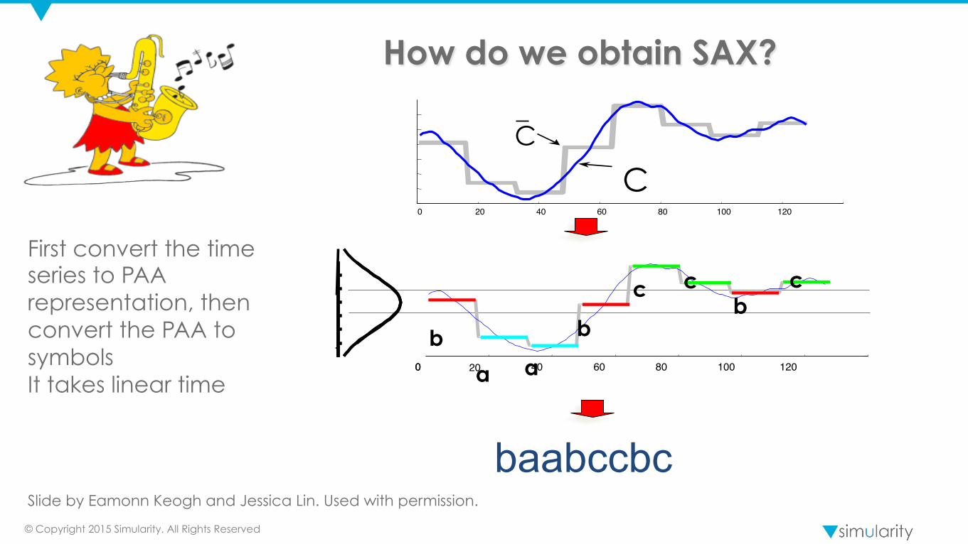
How do we obtain SAX?
First convert the time series to PAA representation, then convert the PAA to symbols It takes linear time
0 20 40 60 80 100 120
C C
Slide by Eamonn Keogh and Jessica Lin. Used with permission.
0
-
-
0 20 40 60 80 100 120
b b
b
a
c
c c
a
baabccbc

© Copyright 2015 Simularity. All Rights Reserved 13 13
Encoding Magnitude And Slope
The Magnitude and slope can be encoded in a SAX word The Magnitude (mean) can be Z-normalized over the entire space of the time series, and divided into SAX letters ! These letters need not be from the same alphabet as the SAX word
which represents the shape, we just need to consider the alphabet size when computing the size of the Finite Symbol Space
Slope can be encoded by dividing 180º into equal spaces, and assigning each space to a letter ! The slope can be determined by a number of methodologies

© Copyright 2015 Simularity. All Rights Reserved 14 14
Computing The Anomaly
We need a data structure, which uses SAX words as an index, and stores the number of times we have seen each SAX word, as well as the total number windows we’ve seen Due to the fact that our SAX words are of a fixed length and alphabet, we know the total number of possible SAX words Tries are one choice of data structure ! Allow for quick access
Converting the SAX word to a number, which is an array index is another ! Requires exponentiation

© Copyright 2015 Simularity. All Rights Reserved 15 15
Computing The Anomaly
The procedure for examining a window ! Convert the window into a SAX word ! Lookup the current count for that SAX word and increment it ! Compute a metric which determines how anomalous the window is
using 3 values – The total number of windows, the number of instances of this SAX word, and the size of the Finite Symbol Space of SAX words
! Compare the result of the metric with a predetermined threshold to decide whether or not this window is anomalous
This procedure is repeated for constantly incoming Time Series Windows

© Copyright 2015 Simularity. All Rights Reserved 16 16
The Metric
Once we have determined the values, we need to turn them into a metric which tells us how anomalous a window is The metric should discriminate ! We should be able to discriminate
between multiple levels of anomaly values
The metric should be easy to compute ! Embedded applications may not have
complex math libraries which allow for complicated computation
The metric should reflect the real world
© Copyright 2015 Simularity. All Rights Reserved 17 17
The Metric – P-Values
P-Values seem like a good metric ! Expressed as a probability, they have a connection to the real world
Unfortunately, P-Values closely approach zero and one once the number of samples gets significant ! This makes it difficult to set an “anomaly threshold” ! This sets a hard criterion for an anomaly

© Copyright 2015 Simularity. All Rights Reserved 18 18
The Metric – Log-Likelihood Ratio
The Log-Likelihood ratio is perhaps a better choice of metric ! Scaling the ratio between -1.0 and 1.0 gives a manageable value ! Even extremely unlikely events can be discriminated
Reversing the sign of the scaled log-likelihood ratio gives values that are easier to understand Use the likelihood function for a binomial distribution ! The number of trials is the Total Windows ! The number of successes is the occurrence of this Window ! The Probability is the Symbol Probability
The log likelihood is particularly useful as it accounts for the significance of the data i.e. the number of samples Like P-Values, it requires a floating point library

© Copyright 2015 Simularity. All Rights Reserved 19 19
The Metric – Rate Ratio
The rate ratio is the number of times more likely the event is observed to have occurred, than would be predicted by random chance ! Smaller values mean more anomalous – less than 1 implies less likely than
chance ! The reciprocal of the rate ratio gives an anomaly score which increases ! Uses observed probabilities
Doesn’t require math harder than division Doesn’t account for significance – significance has to be accounted for by some other means

© Copyright 2015 Simularity. All Rights Reserved 20 20
Other Means Of Symbolizing
SAX may not always be the best way to reduce a window to a symbol ! SAX reduces resolution equally across all its members ! Tiny, but important variations will be lost
Self Organizing Maps can also be used ! They require more computation, but don’t reduce resolution ! Self Organizing Maps can encode magnitude directly

© Copyright 2015 Simularity. All Rights Reserved 21 21
Using Self Organizing Maps
Self Organizing Maps (SOMs) are (typically) a grid of vectors, which can be thought of as weights or prototypes ! The SOM algorithm adjusts the prototypes based on training data
To operate the SOM, a Window vector is compared to each of the prototypes – the best matching one “wins” and the symbol associated with the window is the row:column of the matching grid The row:column is then used to index the count of how many times that prototype has been seen. We now have the 3 values for computing the metric

© Copyright 2015 Simularity. All Rights Reserved 22 22
Predicting Events
A set of time series may be used to predict events ! We look for the correlation between the symbols representing the time
series windows and Events which happen in the future
This can be used to categorize Events according to an Event Signature ! Event signatures imply outcomes at a particular time index

© Copyright 2015 Simularity. All Rights Reserved 23 23
A Concrete Example
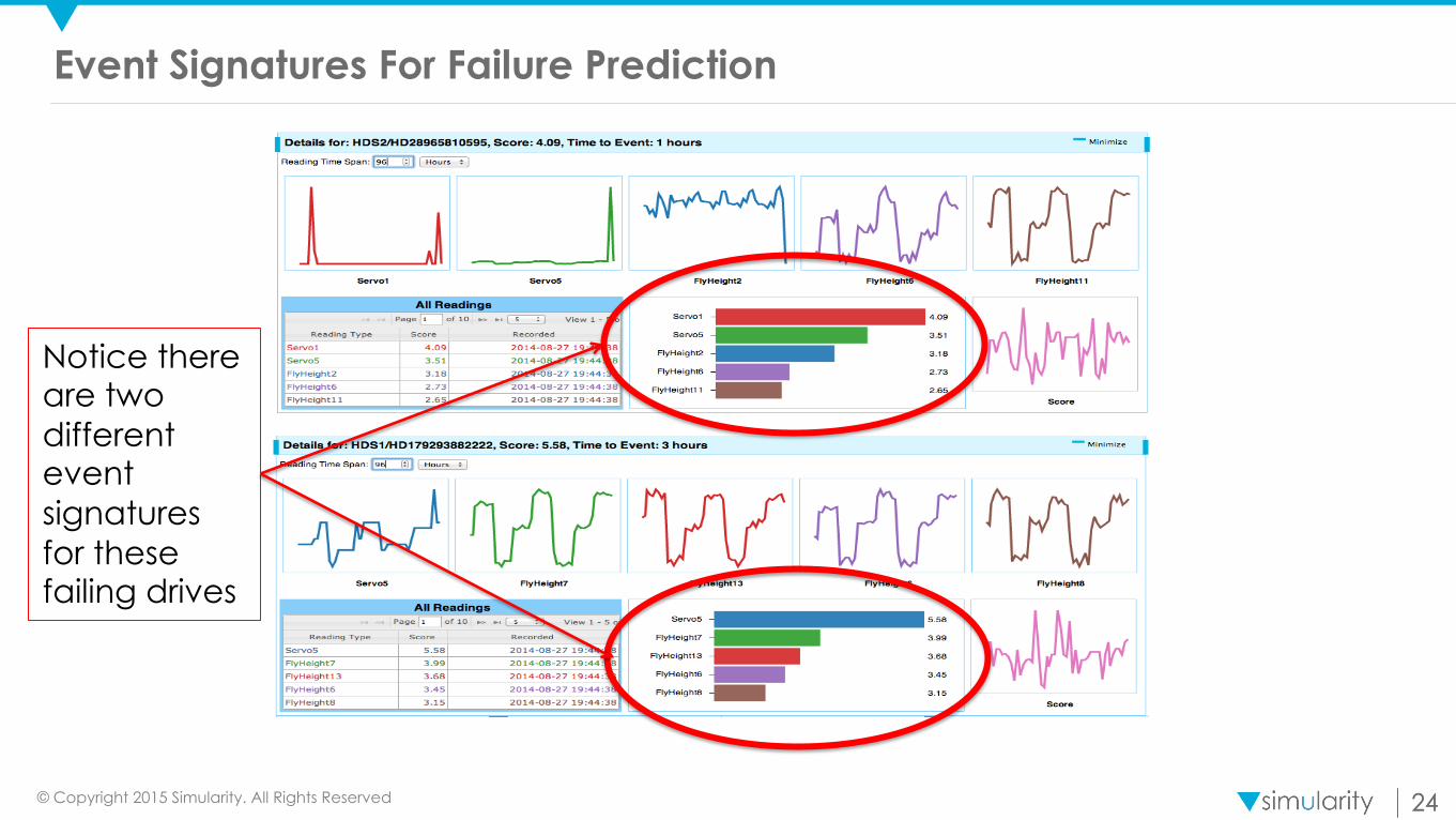
The SMART data on hard drives can be used to predict failures ! Simularity used 53 of the sensors to test for anomalies and predict failures
Information from nearly 400 hard drives was used to “train” the anomaly detector Once trained, the system was used to identify Event Signatures which indicated failure The time series in the system were reduced to SAX words, and correlated with a single event, failure (all that was known) This can then be used to predict failure
© Copyright 2015 Simularity. All Rights Reserved 24 24
Event Signatures For Failure Prediction
Notice there are two different event signatures for these failing drives

© Copyright 2015 Simularity. All Rights Reserved 25 25
Credit
This technique is similar, although not identical, to the TARZAN methodology outlined by Eamonn Keogh and Jessica Lin ! It and other work pertaining to SAX is available here:
http://www.cs.ucr.edu/~eamonn/SAX.htm
Self Organizing Maps were invented by Teuvo Kohonen http://www.cis.hut.fi/research/som-research/teuvo.html

© Copyright 2015 Simularity. All Rights Reserved 26 26
Source Code
Simularity maintains a GitHub repository of open-source software, including an implementation of SAX suitable for using with the techniques described here www.github.com/simularity/SAX

1160, Brickyard Cove Road, Suite 200 Point Richmond, CA 94801 United States
+ 1 678-488-8857
THANK YOU
@rayrichardson


