Hindawi Publishing Corporation Mathematical Problems in Engineering Volume 2011, Article ID 763429, 47 pages doi:10.1155/2011/763429 Research Article Rayleigh Waves in Generalized Magneto-Thermo-Viscoelastic Granular Medium under the Influence of Rotation, Gravity Field, and Initial Stress A. M. Abd-Alla, 1 S. M. Abo-Dahab, 1, 2 and F. S. Bayones 3 1 Mathematics Department, Faculty of Science, Taif University, Taif 21974, Saudi Arabia 2 Mathematics Department, Faculty of Science, South Valley University, Qena 83523, Egypt 3 Mathematics Department, Faculty of Science, Umm Al-Qura University, P.O. Box 10109, Makkah 13401, Saudi Arabia Correspondence should be addressed to S. M. Abo-Dahab, [email protected]Received 4 December 2010; Revised 14 January 2011; Accepted 25 February 2011 Academic Editor: Ezzat G. Bakhoum Copyright q 2011 A. M. Abd-Alla et al. This is an open access article distributed under the Creative Commons Attribution License, which permits unrestricted use, distribution, and reproduction in any medium, provided the original work is properly cited. The surface waves propagation in generalized magneto-thermo-viscoelastic granular medium subjected to continuous boundary conditions has been investigated. In addition, it is also subjected to thermal boundary conditions. The solution of the more general equations are obtained for thermoelastic coupling. The frequency equation of Rayleigh waves is obtained in the form of a determinant containing a term involving the coefficient of friction of a granular media which determines Rayleigh waves velocity as a real part and the attenuation coefficient as an imaginary part, and the effects of rotation, magnetic field, initial stress, viscosity, and gravity field on Rayleigh waves velocity and attenuation coefficient of surface waves have been studied in detail. Dispersion curves are computed numerically for a specific model and presented graphically. Some special cases have also been deduced. The results indicate that the effect of rotation, magnetic field, initial stress, and gravity field is very pronounced. 1. Introduction The dynamical problem in granular media of generalized magneto-thermoelastic waves has been studied in recent times, necessitated by its possible applications in soil mechanics, earthquake science, geophysics, mining engineering, and plasma physics, and so forth. The granular medium under consideration is a discontinuous one and is composed of numerous large or small grains. Unlike a continuous body each element or grain cannot only translate
Transcript
Hindawi Publishing CorporationMathematical Problems in EngineeringVolume 2011, Article ID 763429, 47 pagesdoi:10.1155/2011/763429
Research ArticleRayleigh Waves in GeneralizedMagneto-Thermo-Viscoelastic Granular Mediumunder the Influence of Rotation, Gravity Field, andInitial Stress
A. M. Abd-Alla,1 S. M. Abo-Dahab,1, 2 and F. S. Bayones3
1 Mathematics Department, Faculty of Science, Taif University, Taif 21974, Saudi Arabia2 Mathematics Department, Faculty of Science, South Valley University, Qena 83523, Egypt3 Mathematics Department, Faculty of Science, Umm Al-Qura University, P.O. Box 10109,Makkah 13401, Saudi Arabia
Correspondence should be addressed to S. M. Abo-Dahab, [email protected]
Received 4 December 2010; Revised 14 January 2011; Accepted 25 February 2011
Academic Editor: Ezzat G. Bakhoum
Copyright q 2011 A. M. Abd-Alla et al. This is an open access article distributed under theCreative Commons Attribution License, which permits unrestricted use, distribution, andreproduction in any medium, provided the original work is properly cited.
The surface waves propagation in generalized magneto-thermo-viscoelastic granular mediumsubjected to continuous boundary conditions has been investigated. In addition, it is also subjectedto thermal boundary conditions. The solution of the more general equations are obtained forthermoelastic coupling. The frequency equation of Rayleigh waves is obtained in the form ofa determinant containing a term involving the coefficient of friction of a granular media whichdetermines Rayleigh waves velocity as a real part and the attenuation coefficient as an imaginarypart, and the effects of rotation,magnetic field, initial stress, viscosity, and gravity field on Rayleighwaves velocity and attenuation coefficient of surface waves have been studied in detail. Dispersioncurves are computed numerically for a specific model and presented graphically. Some specialcases have also been deduced. The results indicate that the effect of rotation, magnetic field, initialstress, and gravity field is very pronounced.
1. Introduction
The dynamical problem in granular media of generalized magneto-thermoelastic waves hasbeen studied in recent times, necessitated by its possible applications in soil mechanics,earthquake science, geophysics, mining engineering, and plasma physics, and so forth. Thegranular medium under consideration is a discontinuous one and is composed of numerouslarge or small grains. Unlike a continuous body each element or grain cannot only translate
2 Mathematical Problems in Engineering
but also rotate about its center of gravity. This motion is the characteristic of the mediumand has an important effect upon the equations of motion to produce internal friction. Itwas assumed that the medium contains so many grains that they will never be separatedfrom each other during the deformation and that each grain has perfect thermoelasticity. Theeffect of the granular media on dynamics was pointed out by Oshima [1]. The dynamicalproblem of a generalized thermoelastic granular infinite cylinder under initial stress has beenillustrated by El-Naggar [2]. Rayleigh wave propagation of thermoelasticity or generalizedthermoelasticity was pointed out by Dawan and Chakraporty [3]. Rayleigh waves in amagnetoelastic material under the influence of initial stress and a gravity field were discussedby Abd-Alla et al. [4] and El-Naggar et al. [5].
Rayleigh waves in a thermoelastic granular medium under initial stress on the prop-agation of waves in granular medium are discussed by Ahmed [6]. Abd-Alla and Ahmed[7] discussed the problem of Rayleigh wave propagation in an orthotropic medium undergravity and initial stress. Magneto-thermoelastic problem in rotating nonhomogeneousorthotropic hollow cylinder under the hyperbolic heat conduction model is discussed byAbd-Alla and Mahmoud [8]. Wave propagation in a generalized thermoelastic solid cylinderof arbitrary cross-section is discussed by Venkatesan and Ponnusamy [9]. Some problemsdiscussed the effect of rotation of different materials. Thermoelastic wave propagation ina rotating elastic medium without energy dissipation was studied by Roychoudhuri andBandyopadhyay [10]. Sharma and Grover [11] studied the body wave propagation inrotating thermoelastic media. Thermal stresses in a rotating nonhomogeneous orthotropichollow cylinder were discussed by El-Naggar et al. [12]. Abd-El-Salam et al. [13] investigatedthe numerical solution of magneto-thermoelastic problem nonhomogeneous isotropicmaterial.
In this paper, the effect of magnetic field, rotation, thermal relaxation time, gravityfield, viscosity, and initial stress on propagation of Rayleighwaves in a thermoelastic granularmedium is discussed. General solution is obtained by using Lame’s potential. The frequencyequation of Rayleigh waves is obtained in the form of a determinant. Some special cases havealso been deduced. Dispersion curves are computed numerically for a specific model andpresented graphically. The results indicate that the effect of rotation, magnetic field, initialstress, and gravity field are very pronounced.
2. Formulation of the Problem
Let us consider a system of orthogonal Cartesian axes, Oxyz, with the interface and the freesurface of the granular layer resting on the granular half space of different materials beingthe planes z = K and z = 0, respectively. The origin O is any point on the free surface,the z-axis is positive along the direction towards the exterior of the half space, and the x-axis is positive along the direction of Rayleigh waves propagation. Both media are underinitial compression stress P along the x-direction and the primary magnetic field
−−→H0 acting
on y-axis, as well as the gravity field and incremental thermal stresses, as shown in Figure 1.The state of deformation in the granular medium is described by the displacement vector−→U(u, o,w) of the center of gravity of a grain and the rotation vector
−→ξ (ξ, η, ζ) of the grain
about its center of gravity. The elastic medium is rotating uniformly with an angular velocityΩ = Ωn, where n is a unit vector representing the direction of the axis of rotation. Thedisplacement equation of motion in the rotating frame has two additional terms, Ω × (Ω × u)
Mathematical Problems in Engineering 3
z = K
O
z
Ω
Granularlayer
yP
P
x−−→H0
z = 0
Granularhalf space
g
Figure 1: Depiction of the problem.
is the centripetal acceleration due to time varying motion only, and 2−→Ω ×
−→•u is the Coriolis
acceleration, and Ω = (0,Ω, 0).The electromagnetic field is governed by Maxwell equations, under the consideration
that the medium is a perfect electric conductor taking into account the absence of thedisplacement current (SI) (see the work of Mukhopadhyay [14]):
−→J = curl
−→h,
−μe ∂−→h
∂t= curl
−→E,
div−→h = 0,
div−→E = 0,
−→E = −μe
(∂−→u∂t
× −→H
),
(2.1)
where
−→h = curl
(−→u × −−→H0
),
−→H =
−−→H0 +
−→h,
−−→H0 = (0,H0, 0), (2.2)
where−→h is the perturbed magnetic field over the primary magnetic field vector,
−→E is the
electric intensity,−→J is the electric current density, μe is the magnetic permeability,
−−→H0 is the
constant primary magnetic field vector, and −→u is the displacement vector.The stress and stress couple may be taken to be nonsymmetric, that is, τij /= τji,
Mij /=Mji. The stress tensor τij can be expressed as the sum of symmetric and antisymmetrictensors
τij = σij + σ ′ij , (2.3)
4 Mathematical Problems in Engineering
where
σij =12(τij + τji
), σ ′
ij =12(τij − τji
). (2.4)
The symmetric tensor σij = σji is related to the symmetric strain tensor
eij = eji =12
(∂ui∂xj
+∂uj
∂xi
). (2.5)
The antisymmetric stress σ ′ij are given by
σ ′23 = −F ∂ξ
∂t, σ ′
31 = −F ∂η∂t, σ ′
12 = −F ∂ζ∂t, σ ′
11 = σ′22 = σ
′33 = 0, (2.6)
where F is the coefficient of friction between the individual grains. The stress couple Mij isgiven by
Mij =Mνij , (2.7)
where, M is the third elastic constant, M11, M13, M33, and so forth, are the components ofthe resultant acting on a surface.
The non-symmetric strain tensor νij is defined as
ν11 =∂ξ
∂x, ν31 =
∂ξ
∂z, ν33 =
∂ζ
∂z, ν21 = ν22 = ν23 = 0,
ν12 =∂
∂x
(ω2 + η
), ν32 =
∂
∂z
(ω2 + η
), ν13 =
∂ζ
∂x,
(2.8)
where ω2 = (1/2)((∂u/∂z) − (∂w/∂x)).The dynamic equation of motion, if the magnetic field and rotation are added, can be
written as [15]
τji,j + Fi = ρ[••ui +
{−→Ω ×
(−→Ω × −→u
)}i+
(2−→Ω×
•−→u)i
], i, j = 1, 2, 3. (2.9)
The heat conduction equation is given by [16]
K∇2T = ρs∂
∂t
(1 + τ2
∂
∂t
)T + γT0
∂
∂t
(1 + τ2δ
∂
∂t
)∇ · −→u, (2.10)
where ρ is density of the material,K is thermal conductivity, s is specific heat of the materialper unit mass, τ1, τ2 are thermal relaxation parameter, αt is coefficient of linear thermalexpansion, λ and μ are Lame’s elastic constants, θ is the absolute temperature, γ = αt(3λ+2μ),
Mathematical Problems in Engineering 5
T0 is reference temperature solid, T is temperature difference (θ − T0), τ0 is the mechanicalrelaxation time due to the viscosity, and τm = (1 + τ0(∂/∂t)).
The components of stress in generalized thermoelastic medium are given by
σ11 =[τm
(λ + 2μ
)+ p
]∂u∂x
+ (τmλ + P)∂w
∂z− γ
(1 + τ1
∂
∂t
)T,
σ33 = τmλ∂u
∂x+ τm
(λ + 2μ
)∂w∂z
− γ(1 + τ1
∂
∂t
)T,
σ13 = τmμ(∂u
∂z+∂w
∂x
).
(2.11)
If we neglect the thermal relaxation time, then (2.11) tends to Nowacki [17] and Biot [18].The Maxwell’s electro-magnetic stress tensor τij is given by
τij = μe[Hihj +Hjhi − (Hk · hk)δij
], i, j = 1, 2, 3, (2.12)
which takes the form
τ11 = −μeH20∇2φ, τ13 = τ23 = 0, τ33 = μeH2
0∇2φ, ∇2φ =∂u
∂x+∂w
∂z. (2.13)
The dynamic equations of motion are
∂τ11∂x
+∂τ31∂z
+P
2∂ω2
∂z− ρg ∂w
∂x+ Fx = ρ
[∂2u
∂t2+ 2Ω
∂w
∂t−Ω2u
],
∂τ12∂x
+∂τ32∂z
+ Fy = 0,
∂τ13∂x
+∂τ33∂z
+P
2∂ω2
∂x+ ρg
∂w
∂x+ Fz = ρ
[∂2w
∂t2− 2Ω
∂u
∂t−Ω2w
],
(2.14)
where g is the Earth’s gravity and
�F =(−μeH2
0∇2φ, 0, μeH20∇2φ
), (2.15)
τ23 − τ32 + ∂M11
∂x+∂M31
∂z= 0,
τ31 − τ13 + ∂M12
∂x+∂M32
∂z= 0,
τ12 − τ21 + ∂M13
∂x+∂M33
∂z= 0.
(2.16)
6 Mathematical Problems in Engineering
From (2.3)–(2.8) and (2.11), we have
τ11 =[τm
(λ + 2μ
)+ p
]∂u∂x
+ (τmλ + P)∂w
∂z− γ
(1 + τ1
∂
∂t
)T,
τ33 = τmλ∂u
∂x+ τm
(λ + 2μ
)∂w∂z
− γ(1 + τ1
∂
∂t
)T,
τ13 = τmμ(∂u
∂z+∂w
∂x
)+ F
∂η
∂t,
τ12 = −F ∂ζ∂t,
τ23 = −F ∂ξ∂t,
M11 =M∂ξ
∂x, M31 = M
∂ξ
∂z, M33 =M
∂ζ
∂z, M21 =M22 =M23 = 0,
M12 =M∂
∂x
(ω2 + η
), M32 = M
∂
∂z
(ω2 + η
), M13 =M
∂ζ
∂x.
(2.17)
Substituting (2.17) into (2.14) and (2.16) tends to
[τm
(λ + 2μ
)+ P
]∂2u∂x2
+ (τmλ + P)∂2w
∂x ∂z− γ
(1 + τ1
∂
∂t
)∂T
∂x+ τmμ
(∂2u
∂z2+
∂2w
∂x∂z
)
+P
2
(∂2u
∂z2− ∂2w
∂x∂z
)− ρg ∂w
∂x+ F
∂2η
∂z ∂t+μeH2
0
(∂2u
∂x2+
∂2w
∂x∂z
)=ρ
[∂2u
∂t2+2Ω
∂w
∂t−Ω2u
],
(2.18)
then
[τm
(λ + 2μ
)+ P + μeH2
0
]∂2u∂x2
+[τm
(λ + μ
)+P
2+ μeH2
0
]∂2w
∂x∂z+
(τmμ +
P
2
)∂2u
∂z2
− γ(1 + τ1
∂
∂t
)∂T
∂x− ρg ∂w
∂x+ F
∂2η
∂z ∂t= ρ
[∂2u
∂t2+ 2Ω
∂w
∂t−Ω2u
].
(2.19)
Mathematical Problems in Engineering 7
Also,
∂
∂t
(∂ζ
∂x− ∂ξ
∂z
)= 0, (2.20)
τmμ
(∂2u
∂x ∂z+∂2w
∂x2
)− F ∂2η
∂x ∂t+ τmλ
∂2u
∂x ∂z+ τm
(λ + 2μ
)∂2w∂z2
− γ(1 + τ1
∂
∂t
)∂T
∂z
+P
2
(∂2u
∂x ∂z− ∂2w
∂x2
)+ ρg
∂u
∂x+ μeH2
0
(∂2u
∂x ∂z+∂2w
∂z2
)= ρ
[∂2w
∂t2− 2Ω
∂u
∂t−Ω2w
],
(2.21)
then
[τm
(λ + μ
)+P
2+ μeH2
0
]∂2u
∂x ∂z+
(τmμ − P
2
)∂2w
∂x2+
[τm
(λ + 2μ
)+ μeH2
0
]∂2w∂z2
− γ(1 + τ1
∂
∂t
)∂T
∂z+ ρg
∂u
∂x− F ∂2η
∂x ∂t= ρ
[∂2w
∂t2− 2Ω
∂u
∂t−Ω2w
],
(2.22)
and, from (2.16), we have
∇2ξ − s2 ∂ξ∂t
= 0, (2.23)
∇2(ω2 + η) − s2 ∂η
∂t= 0, (2.24)
∇2ζ − s2 ∂ζ∂t
= 0, (2.25)
where
s2 =2FM
. (2.26)
3. Solution of the Problem
By Helmholtz’s theorem [19], the displacement vector −→u can be written in the displacementpotentials φ and ψ form, as
−→u = grad φ + curl −→ψ, −→ψ =(0, ψ, 0
), (3.1)
which reduces to
u =∂φ
∂x− ∂ψ
∂z, w =
∂φ
∂z+∂ψ
∂x. (3.2)
8 Mathematical Problems in Engineering
Substituting (3.2) into (2.19), (2.22), and (2.24), the wave equations tend to
α2∇2φ − γ
ρ
(1 + τ1
∂
∂t
)T − g ∂ψ
∂x=∂2φ
∂t2+ 2Ω
∂ψ
∂t−Ω2φ, (3.3)
β2∇2ψ − s1∂η
∂t+ g
∂φ
∂x=∂2ψ
∂t2− 2Ω
∂φ
∂t−Ω2ψ, (3.4)
∇2η − s2∂η
∂t− ∇4ψ = 0, (3.5)
where
s1 =F
ρ, α2 =
τm(λ + 2μ
)+ P + μeH2
0
ρ, β 2 =
2τmμ − P2ρ
. (3.6)
Substituting (3.2) into (2.10), we obtain
K∇2T = ρs∂
∂t
(1 + τ2
∂
∂t
)T + γT0
∂
∂t
(1 + τ2δ
∂
∂t
)∇2φ. (3.7)
From (3.3) and (3.7), by eliminating T , we obtain
[∇2 − 1
χ
∂
∂t
(1 + τ2
∂
∂t
)][α2∇2φ − g ∂ψ
∂x− ∂2φ
∂t2− 2Ω
∂ψ
∂t+ Ω2φ
]
− ε ∂∂t
(1 + τ1
∂
∂t
)(1 + τ2δ
∂
∂t
)∇2φ = 0,
(3.8)
where
χ =K
ρs, ε =
γ2T0ρK
. (3.9)
From (3.4) and (3.5) by eliminating η, we obtain
(∇2 − s2 ∂
∂t
)(β2∇2ψ − ∂2ψ
∂t2+ g
∂φ
∂x+ 2Ω
∂φ
∂t+ Ω2ψ
)− s1∇4 ∂ψ
∂t= 0. (3.10)
For a plane harmonic wave propagation in the x-direction, we assume
φ = φ1eik(x−ct), ψ = ψ1e
ik(x−ct), (3.11)(ξ, η, ζ
)=
(ξ1, η1, ζ1
)eik(x−ct). (3.12)
Mathematical Problems in Engineering 9
From (3.12) into (2.20), (2.23), and (2.25), we get
Dξ1 − ikζ1 = 0, (3.13)
D2ξ1 + q2ξ1 = 0, (3.14)
D2ζ1 + q2ζ1 = 0, (3.15)
where
q2 = ikcs2 − k2, D ≡ d
dz. (3.16)
The solution of (3.14) and (3.15) takes the form
ξ1 = A1eiqz +A2e
−iqz, ζ1 = B1eiqz + B2e
−iqz, (3.17)
where A1, A2, B1, and B2 are arbitrary constants.From (3.13) and (3.17), we obtain
q(A1e
iqz −A2e−iqz
)− k
(B1e
iqz + B2e−iqz
)= 0, (3.18)
then
qA1 − kB1 = 0,
qA2 − kB2 = 0
}=⇒ Aj =
(−1)j−1kq
Bj , j = 1, 2. (3.19)
Substituting (3.11) into (3.8) and (3.10), we obtain
where the constants Ej and Fj are related to the constants Cj andDj in the form
Ej = mjCj , Fj = mjDj, j = 1, 2, 3, 4,
mj =1(
g − 2Ωc)(ikN2
j − ik − (εΓ2/χ
))
×{α2∗k
2N4j −
[k2
(c2 − 2α2∗
)+ikc
χ
(α2∗Γ2 + χεΓ1Γ3
)+ Ω2
]N2
j
+ikcΓ2χ
(1 − α2∗ +
Ω2
k2
)−
(Ω2 + ikεcΓ1Γ3
)}.
(3.23)
Substituting (3.22) into (3.11), we obtain
φ =4∑j=1
[Cje
ikNjz +Dje−ikNjz
]eik(x−ct),
ψ =4∑j=1
[Eje
ikNjz + Fje−ikNjz]eik(x−ct),
(3.24)
Mathematical Problems in Engineering 11
and values of displacement components u and w are
u = ik4∑j=1
[(1 −Njmj
)Cje
ikNjz +(1 +Njmj
)Dje
−ikNjz]eik(x−ct),
w = ik4∑j=1
[(Nj +mj
)Cje
ikNjz +(mj −Nj
)Dje
−ikNjz]eik(x−ct),
(3.25)
whereN1,N2,N3, andN4 are taken to be the complex roots of the following equation
N8 + t1N6 + t2N4 + t3N2 + t4 = 0, (3.26)
where
t1 =k2
α2∗
(c2 − 2α2∗
)+ikc
α2∗χ
(α2∗Γ2 + χεΓ1Γ3
)+ Ω2 +
1β2∗ + ikcs1
×[k2
(c2 − 2β2∗
)+ ikc
(s2β
2∗ − 2k2s1
)+ Ω2
],
(3.27)
t2 =1α2∗
[k4
(α2∗ − c2
)+ikcΓ2χ
(k2
(1 − α2∗
)+ Ω2
)− k2
(Ω2 + ikεcΓ1Γ3
)]
+1
α2∗(β2∗ + ikcs1
)[k2
(c2 − 2β2∗
)+ ikc
(s2β
2∗ − 2k2s1
)+ Ω2
]
×[k2
(c2 − 2α2∗
)+ikc
χ
(α2∗Γ2 + χεΓ1Γ3
)+ Ω2
]
+1(
β2∗ + ikcs1)[k2
(k2 − ikcs2
)(β2∗ − c2
)+ ikc
(s2Ω2 + k4s1
)]
− 1α2∗
(β2∗ + ikcs1
)[k2
(g − 2Ωc
)2],
(3.28)
t3 =1
α2∗(β2∗ + ikcs1
)
×{[k2
(c2 − 2β2∗
)+ ikc
(s2β
2∗ − 2k2s1
)+ Ω2
]
×[k4
(α2∗ − c2
)+ikcΓ2χ
(k2
(1 − α2∗
)+ Ω2
)− k2
(Ω2 + ikεcΓ1Γ3
)]
12 Mathematical Problems in Engineering
+[k2
(k2 − ikcs2
)(β2∗ − c2
)+ ikc
(s2Ω2 + k4s1
)]
×[k2
(c2 − 2α2∗
)+ikc
χ
(α2∗Γ2 + χεΓ1Γ3
)+ Ω2
]
−[ik
(g − 2Ωc
)2(ik3 +
k2cΓ2χ
)]− ik3
[(g − 2Ωc
)2(ik − cs2)]},
(3.29)
t4 =1
α2∗(β2∗ + ikcs
)
×{[k2
(k2 − ikcs2
)(β2∗ − c2
)+ ikc
(s2Ω2 + k4s1
)]× [
ik(g − 2Ωc
)]
+
[(2Ωc − g)2(ik3 − k2cs2)
(ik3 +
k2cΓ2χ
)]}.
(3.30)
From (3.4), (3.11), (3.12), (3.22), and (3.23), we obtain
η1 =4∑j=1
1ikcs1
{k2β2∗mj
(1 +N2
j
)−mj
(k2c2 + Ω2
)+ ik
(2Ωc − g)} ×
[Cje
ikNjz +Dje−ikNjz
].
(3.31)
Using (3.22) and (3.11) into (3.3), we obtain
T =ρ
γΓ1
4∑j=1
[−α2∗k2
(1 +N2
j
)+ k2c2 − ikgmj
](Cje
ikNjz +Dje−ikNjz
)eik(x−ct). (3.32)
With the lower medium, we use the symbols with primes, for ξ1, ζ1, η1, T, φ, ψ, and q,for z > K,
ξ′1 = − kq′B′2e
−iq′z, ζ′1 = B′2e
−iq′z,
η′1 =4∑j=1
1ikcs′1
{k2β
′2∗ m
′j
(1 +N
′2j
)−m′
j
(k2c2 + Ω
′2)+ ik
(2Ω′c − g)}D′
je−ikN′
j z,
T ′ =ρ′
γ ′Γ1
4∑j=1
[−α′2
∗ k2(1 +N
′2j
)+ k2c2 − ikgm′
j
]D′je
−ikN′jzeik(x−ct),
Mathematical Problems in Engineering 13
φ′ =4∑j=1
D′je
−ikN′jzeik(x−ct),
ψ ′ =4∑j=1
F ′je
−ikN′jzeik(x−ct).
(3.33)
4. Boundary Conditions and Frequency Equation
In this section, we obtain the frequency equation for the boundary conditions which arespecific to the interface z = K, that is,
(i) u = u′,
(ii) w = w′,
(iii) ξ = ξ′,
(iv) η = η′,
(v) ζ = ζ′,
(vi) M33 =M′33,
(vii) M31 =M′31,
(viii) M32 =M′32,
(ix) τ33 + τ33 = τ ′33 + τ′33
(x) τ31 + τ31 = τ ′31 + τ′31,
(xi) τ32 + τ32 = τ ′32 + τ′32,
(xii) T = T ′,
(xiii) (∂T/∂z) + θT = (∂T ′/∂z) + θT ′.
The boundary conditions on the free surface z = 0 are
(xiv) M33 = 0,
(xv) M31 = 0,
(xvi) M32 = 0,
(xvii) τ33 + τ33 = 0,
(xviii) τ31 + τ31 = 0,
(xix) τ32 + τ32 = 0,
(xx) (∂T/∂z) + θT = 0.
14 Mathematical Problems in Engineering
From conditions (iii), (v), (vi), and (vii), we obtain
B1eiqK − B2e
−iqK = −B′2e
−iq′K,
B1eiqK + B2e
−iqK = B′2e
−iq′K,
M(B1e
iqK − B2e−iqK
)= −M′B′
2e−iq′K,
M(B1e
iqK + B2e−iqK
)= −M′B′
2e−iq′K.
(4.1)
Hence,
B1 = B2 = B′2 = 0, ξ = ζ = ξ′ = ζ′ = 0. (4.2)
The other significant boundary conditions are responsible for the following relations:
(i)
4∑j=1
(1 −Njmj
)Cje
ikNjK +(1 +Njmj
)Dje
−ikNjK −(1 +N ′
jm′j
)D′je
−ikN′jK = 0, (4.3)
(ii)
4∑j=1
(Nj +mj
)Cje
ikNjK +(mj −Nj
)Dje
−ikNjK −(m′j −N ′
j
)D′je
−ikN′jK = 0, (4.4)
(iv)
4∑j=1
1cs1
{k2β2∗mj
(1 +N2
j
)−mj
(k2c2 + Ω2
)+ ik
(2Ωc − g)} ×
[Cje
ikNjK +Dje−ikNjK
]
−4∑j=1
1cs′1
{k2β
′2∗ m
′j
(1 +N
′2j
)−m′
j
(k2c2 + Ω
′2)+ ik
(2Ω′c − g)}D′
je−ikN′
jK = 0,
(4.5)
Mathematical Problems in Engineering 15
(viii)
MNj
4∑j=1
{k2mj
(N2
j + 1)+
1ikcs1
(k2β2∗mj
(1 +N2
j
)−mj
(k2c2 + Ω2
)+ ik
(2Ωc − g))}
×[Cje
ikNjK −Dje−ikNjK
]
+M′N ′j
4∑j=1
{k2m′
j
(N
′2j + 1
)+
1ikcs′1
×(k2β
′2∗ m
′j
(1 +N
′2j
)−m′
j
(k2c2 + Ω
′2)+ ik
(2Ω′c − g))
}D′je
−ikN′jK = 0,
(4.6)
(ix)
4∑j=1
{[(Γ0λ + μeH2
0
)(1 −Njmj
)+
(Γ0
(λ + 2μ
)+ μeH2
0
)(N2
j +mjNj
)]
× CjeikNjK +
[(Γ0λ + μeH2
0
)(1 +Njmj
)+
(Γ0
(λ + 2μ
)+ μeH2
0
)(N2
j −mjNj
)]
×Dje−ikNjK + ρ
[−α2∗
(1 +N2
j
)+ c2 − ig
kmj
][Cje
ikNjK +Dje−ikNjK
]
−[(
Γ′0λ′ + μ′eH
20
)(1 +N ′
jm′j
)+
(Γ′0
(λ′ + 2μ′
)+ μ′eH
20
)(N
′2j −m′
jN′j
)]D′je
−ikN′jK
−ρ′[−α′2
∗(1 +N
′2j
)+ c2 − ig
km′j
]D′je
−ikN′jK
}= 0,
(4.7)
(x)
4∑j=1
{−2k2Γ0μNj
[Cje
ikNjK −Dje−ikNjK
]
+[−k2Γ0μmj
(1 −N2
j
)+F
s1
{k2β2∗mj
(1 +N2
j
)−mj
(k2c2 + Ω2
)+ ik
(2Ωc − g)}]
×[Cje
ikNjK +Dje−ikNjK
]− 2k2Γ′0μ
′N ′jD
′je
−ikN′jK
−[−k2Γ′0μ′m′
j
(1 −N ′2
j
)+F
s′1
{k2β
′2∗ m
′j
(1 +N
′2j
)−m′
j
(k2c2 + Ω
′2)+ ik
(2Ω′c − g)}
]
×D′je
−ikN′jK
}= 0,
(4.8)
16 Mathematical Problems in Engineering
(xii)
4∑j=1
ρ
γ
[−α2∗k2
(N2
j + 1)+ k2c2 − igkmj
][Cje
ikNjK +Dje−ikNjK
]
− ρ′
γ ′[−α′2
∗ k2(N
′2j + 1
)+ k2c2 − igkm′
j
]D′je
−ikN′jK = 0,
(4.9)
(xiii)
4∑j=1
ρ
γ
[−α2∗k2
(N2
j + 1)+ k2c2 − igkmj
][(θ + ikNj
)Cje
ikNjK +(θ − ikNj
)Dje
−ikNjK]
− ρ′
γ ′[−α′2
∗ k2(N
′2j + 1
)+ k2c2 − igkm′
j
]×
(θ − ikN ′
j
)D′je
−ikNj ′K = 0,
(4.10)
(xvi)
MNj
4∑j=1
{k2mj
(N2
j + 1)+
1ikcs1
(k2β2∗mj
(1 +N2
j
)−mj
(k2c2 + Ω2
)+ ik
(2Ωc − g))}
× [Cj −Dj
]= 0,
(4.11)
(xvii)
4∑j=1
{[(Γ0λ + μeH2
0
)(1 −Njmj
)+
(Γ0
(λ + 2μ
)+ μeH2
0
)(N2
j +mjNj
)]Cj
+[(
Γ0λ + μeH20
)(1 +Njmj
)+
(Γ0
(λ + 2μ
)+ μeH2
0
)(N2
j −mjNj
)]Dj
+ρ[−α2∗
(1 +N2
j
)+ c2 − ig
kmj
][Cj +Dj
]}= 0,
(4.12)
(xviii)
4∑j=1
{−2k2Γ0μNj
[Cj −Dj
]
+[−k2Γ0μmj
(1 −N2
j
)+F
s1
{k2β2∗mj
(1 +N2
j
)−mj
(k2c2 + Ω2
)+ ik
(2Ωc − g)}]
×[Cj +Dj
]}= 0,
(4.13)
Mathematical Problems in Engineering 17
(xx)
4∑j=1
[−α2∗k2
(N2
j + 1)+ k2c2 − igkmj
][(θ + ikNj
)Cj +
(θ − ikNj
)Dj
]= 0. (4.14)
5. Special Cases and Discussion
5.1. The Magnetic Field, Initial Stress, and Thermal Relaxation Time AreNeglected
In this case (i.e.,H0 = 0, p = 0, and τ1 = τ2 = 0), (3.26) tends to
V 8 + h1V 6 + h2V 4 + h3V 2 + h4 = 0, (5.1)
where
α2∗ =Γ0
(λ + 2μ
)ρ
, β2∗ =Γ0μρ,
mj =1(
g − 2Ωc)(ikV 2
j − ik − (ε/χ
))
×{α2∗k
2V 4j −
[k2
(c2 − 2α2∗
)+ikc
χ
(α2∗ + χε
)+ Ω2
]V 2j +
ikc
χ
(1 − α2∗ +
Ω2
k2
)−
(Ω2 + ikεc
)},
h1 =k2
α2∗
(c2 − 2α2∗
)+ikc
α2∗χ
(α2∗ + χε
)+ Ω2 +
1β2∗ + ikcs1
×[k2
(c2 − 2β2∗
)+ ikc
(s2β
2∗ − 2k2s1
)+ Ω2
],
h2 =1α2∗
[k4
(α2∗ − c2
)+ikc
χ
(k2
(1 − α2∗
)+ Ω2
)− k2
(Ω2 + ikεc
)]
+1
α2∗(β2∗ + ikcs1
)[k2
(c2 − 2β2∗
)+ ikc
(s2β
2∗ − 2k2s1
)+ Ω2
]
×[k2
(c2 − 2α2∗
)+ikc
χ
(α2∗ + χε
)+ Ω2
]
+1(
β2∗ + ikcs1)[k2
(k2 − ikcs2
)(β2∗ − c2
)+ ikc
(s2Ω2 + k4s1
)]
− 1α2∗
(β2∗ + ikcs1
)[k2
(g − 2Ωc
)2],
18 Mathematical Problems in Engineering
h3 =1
α2∗(β2∗ + ikcs1
){[k2
(c2 − 2β2∗
)+ ikc
(s2β
2∗ − 2k2s1
)+ Ω2
]
×[k4
(α2∗ − c2
)+ikc
χ
(k2
(1 − α2∗
)+ Ω2
)− k2
(Ω2 + ikεc
)]
+[k2
(k2 − ikcs2
)(β2∗ − c2
)+ ikc
(s2Ω2 + k4s1
)]
×[k2
(c2 − 2α2∗
)+ikc
χ
(α2∗ + χε
)+ Ω2
]
−[ik
(g − 2Ωc
)2(ik3 +
k2c
χ
)]− ik3
[(g − 2Ωc
)2(ik − cs2)]},
h4 =1
α2∗(β2∗ + ikcs
){[k2
(k2 − ikcs2
)(β2∗ − c2
)+ ikc
(s2Ω2 + k4s1
)]× [
ik(g − 2Ωc
)]
+
[(2Ωc − g)2(ik3 − k2cs2)
(ik3 +
k2c
χ
)]}.
(5.2)
Also,
η1 =4∑j=1
1ikcs1
{k2β2∗mj
(1 + V 2
j
)−mj
(k2c2 + Ω2
)+ ik
(2Ωc − g)} ×
[Cje
ikVjz +Dje−ikVjz
].
T =ρ
γ
4∑j=1
[−α2∗k2
(1 + V 2
j
)+ k2c2 − ikgmj
](Cje
ikVjz +Dje−ikVjz
)eik(x−ct),
ξ′1 = − kq′B′2e
−iq′z, ζ′1 = B′2e
−iq′z,
η′1 =4∑j=1
1ikcs′1
{k2β
′2∗ m
′j
(1 + V
′2j
)−m′
j
(k2c2 + Ω
′2)+ ik
(2Ω′c − g)}D′
je−ikV ′
j z,
T ′ =ρ′
γ ′
4∑j=1
[−α′2
∗ k2(1 + V
′2j
)+ k2c2 − ikgm′
j
]D′je
−ikV ′j zeik(x−ct),
φ′1 =
4∑j=1
D′je
−ikV ′j z,
ψ ′1 =
4∑j=1
F ′je
−ikV ′j z,
(5.3)
Mathematical Problems in Engineering 19
Using the boundary conditions, we obtain
⎡⎢⎢⎢⎢⎢⎣
d11 d12 · · · d18 d′15 d′
16 · · · d′18
d21 d22 · · · d28 d′25 d′
26 · · · d′28
......
......
......
......
d121 d122 · · · d128 d′125 d′
126 · · · d′128
⎤⎥⎥⎥⎥⎥⎦
⎡⎢⎢⎢⎢⎢⎢⎢⎢⎢⎢⎢⎢⎢⎢⎢⎢⎢⎢⎢⎢⎢⎢⎢⎢⎢⎢⎢⎢⎢⎢⎣
C1
C2
C3
C4
D1
D2
D3
D4
D′1
D′2
D′3
D′4
⎤⎥⎥⎥⎥⎥⎥⎥⎥⎥⎥⎥⎥⎥⎥⎥⎥⎥⎥⎥⎥⎥⎥⎥⎥⎥⎥⎥⎥⎥⎥⎦
= [0], (5.4)
where
d1j =(1 − Vjmj
)Cje
ikVj K +(1 + Vjmj
)Dje
−ikVj K, d′1j =
(1 + V ′
jm′j
)D′je
−ikV ′j K,
d2j =(Vj +mj
)Cje
ikVj K +(mj − Vj
)Dje
−ikVj K, d′2j =
(m′j − V ′
j
)D′je
−ikV ′j K,
d3j =1cs1
{k2β2∗mj
(1 + V 2
j
)−mj
(k2c2 + Ω2
)+ ik
(2Ωc − g)}[
CjeikVjz +Dje
−ikVjz],
d′3j =
1cs′1
{k2β
′2∗ m
′j
(1 + V
′2j
)−m′
j
(k2c2 + Ω2
)+ ik
(2Ωc − g)}D′
je−ikV ′
j z,
d4j = MVj
{k2mj
(V 2j + 1
)+
1ikcs1
(k2β2∗mj
(1 + V 2
j
)−mj
(k2c2 + Ω2
)+ ik
(2Ωc − g))
×[Cje
ikVjK −Dje−ikVjK
],
d′4j = M
′V ′j
{k2m′
j
(V
′2j + 1
)+
1ikcs′1
(k2β
′2∗ m
′j
(1 + V
′2j
)−m′
j
(k2c2 + Ω2
)+ ik
(2Ωc − g))
}
×D′je
−ikV ′jK,
d5j =[Γ0λ
(1 − Vjmj
)+ Γ0
(λ + 2μ
)(V 2j +mjVj
)]Cje
ikVjK
+[Γ0λ
(1 + Vjmj
)+ Γ0
(λ + 2μ
)(V 2j −mjVj
)]Dje
−ikVjK
+ ρ[−α2∗
(1 + V 2
j
)+ c2 − ig
kmj
][Cje
ikVjK +Dje−ikVjK
],
20 Mathematical Problems in Engineering
d′5j =
[Γ′0λ
′(1 + V ′
jm′j
)+ Γ′0
(λ′ + 2μ′
)(V
′2j −m′
jV′j
)]D′je
−ikV ′j K + ρ′
[−α′2
∗(1 + V
′2j
)+ c2 − ig
km′j
]
×D′je
−ikV ′jK
},
d6j = −2k2Γ0μVj[Cje
ikVjK −Dje−ikVjK
]+
[−k2Γ0μmj
(1 − V 2
j
)+F
s1
{k2β2∗mj
(1 + V 2
j
)−mj
(k2c2 + Ω2
)+ ik
(2Ωc − g)}]
×[Cje
ikVjK +Dje−ikVjK
],
d′6j = 2k2Γ′0μ
′V ′jD
′je
−ikV ′j K
+
[−k2Γ′0μ′m′
j
(1 − V ′2
j
)+F
s′1
{k2β
′2∗ m
′j
(1 + V
′2j
)−m′
j
(k2c2 + Ω2
)+ ik
(2Ωc − g)}
]
×D′je
−ikV ′jK,
d7j =ρ
γ
[−α2∗k2
(V 2j + 1
)+ k2c2 − igkmj
][Cje
ikVjK +Dje−ikVjK
],
d′7j =
ρ′
γ ′[−α′2
∗ k2(V
′2j + 1
)+ k2c2 − igkm′
j
]D′je
−ikV ′j K,
d8j =ρ
γ
[−α2∗k2
(V 2j + 1
)+ k2c2 − igkmj
][(θ + ikVj
)Cje
ikVjK +(θ − ikVj
)Dje
−ikVjK],
d′8j =
ρ′
γ ′[−α′2
∗ k2(V
′2j + 1
)+ k2c2 − igkm′
j
](θ − ikV ′
j
)D′je
−ikV ′j K,
d9j = MVj
{k2mj
(V 2j + 1
)+
1ikcs1
(k2β2∗mj
(1 + V 2
j
)−mj
(k2c2 + Ω2
)+ ik
(2Ωc − g))}
× [Cj −Dj
],
d10j =[Γ0λ
(1 − Vjmj
)+ Γ0
(λ + 2μ
)(V 2j +mjVj
)]Cj
+[Γ0λ
(1 + Vjmj
)+ Γ0
(λ + 2μ
)(V 2j −mjVj
)]Dj
+ ρ[−α2∗
(1 + V 2
j
)+ c2 − ig
kmj
][Cj +Dj
],
d11j = −2k2Γ0μVj[Cj −Dj
]+
[−k2Γ0μmj
(1 − V 2
j
)+F
s1
{k2β2∗mj
(1 + V 2
j
)−mj
(k2c2 + Ω2
)+ ik
(2Ωc − g)}]
× [Cj +Dj
],
d12j =[−α2∗k2
(V 2j + 1
)+ k2c2 − igkmj
][(θ + ikVj
)Cj +
(θ − ikVj
)Dj
],
d′9j = d
′10j = d
′11j = d
′12j = 0, j = 1, 2, 3, 4.
(5.5)
Mathematical Problems in Engineering 21
5.2. The Magnetic Field, Initial Stress, Rotation, and Thermal RelaxationTime Are Neglected and in Viscoelastic Medium
In this case (i.e.,H0 = 0, P = 0, Ω = 0, and τ0 = τ1 = τ2 = 0), the previous results obtained asin Abd-Alla et al. [20].
5.3. Absence of the Gravity Field
In this case, we put g = 0, then (3.20) becomes
[α2∗D
4 +G1D2 +G2
]φ1 −
[G∗
3D2 +G∗
4
]ψ1 = 0,
[R1D
4 + R2D2 + R3
]ψ1 +
[R∗4D
2 + R∗5
]φ1 = 0,
(5.6)
where
G∗3 = −2ikΩc, G∗
4 = 2Ωc
(ik3 +
k2cΓ2χ
),
R∗4 = −2ikΩc, R∗
5 = 2Ωc(ik3 − k2cs2
),
(5.7)
and G1, G2, R1, R2, and R3 are as in (3).The solution of (5.6) take the form
φ =4∑j=1
[C∗j e
ikXjz +D∗j e
−ikXjz]eik(x−ct),
ψ =4∑j=1
[E∗j e
ikXjz + F∗j e
−ikXjz]eik(x−ct),
(5.8)
where
E∗j = m
∗j C
∗j , F∗
j = m∗jD
∗j , j = 1, 2, 3, 4, (5.9)
m∗j =
1
−2Ωc(ikX2
j − ik − ((εΓ2)/χ
))
×{α2∗k
2X4j −
[k2
(c2 − 2α2∗
)+ikc
χ
(α2∗Γ2 + χεΓ1Γ3
)+ Ω2
]X2j
+ikcΓ2χ
(1 − α2∗ +
Ω2
k2
)−
(Ω2 + ikεcΓ1Γ3
)},
(5.10)
22 Mathematical Problems in Engineering
and X1, X2, X3, and X4 are taken to be the complex roots of equation
X8 + t∗1X6 + t∗2X
4 + t∗3X2 + t∗4 = 0, (5.11)
where
t∗1 =k2
α2∗
(c2 − 2α2∗
)+ikc
α2∗χ
(α2∗Γ2 + χεΓ1Γ3
)+ Ω2 +
1β2∗ + ikcs1
×[k2
(c2 − 2β2∗
)+ ikc
(s2β
2∗ − 2k2s1
)+ Ω2
],
t∗2 =1α2∗
[k4
(α2∗ − c2
)+ikcΓ2χ
(k2
(1 − α2∗
)+ Ω2
)− k2
(Ω2 + ikεcΓ1Γ3
)]
+1
α2∗(β2∗ + ikcs1
)[k2
(c2 − 2β2∗
)+ ikc
(s2β
2∗ − 2k2s1
)+ Ω2
]
×[k2
(c2 − 2α2∗
)+ikc
χ
(α2∗Γ2 + χεΓ1Γ3
)+ Ω2
]
+1(
β2∗ + ikcs1)[k2
(k2 − ikcs2
)(β2∗ − c2
)+ ikc
(s2Ω2 + k4s1
)]
− 1α2∗
(β2∗ + ikcs1
)[4k2Ω2c2
],
t∗3 =1
α2∗(β2∗ + ikcs1
)
×{[k2
(c2 − 2β2∗
)+ ikc
(s2β
2∗ − 2k2s1
)+ Ω2
]
×[k4
(α2∗ − c2
)+ikcΓ2χ
(k2
(1 − α2∗
)+ Ω2
)− k2
(Ω2 + ikεcΓ1Γ3
)]
+[k2
(k2 − ikcs2
)(β2∗ − c2
)+ ikc
(s2Ω2 + k4s1
)]
×[k2
(c2 − 2α2∗
)+ikc
χ
(α2∗Γ2 + χεΓ1Γ3
)+ Ω2
]
−4Ω2c2[ik
(ik3 +
k2cΓ2χ
)+ ik3(ik − cs2)
]},
Mathematical Problems in Engineering 23
t∗4 =1
α2∗(β2∗ + ikcs
){[k2
(k2 − ikcs2
)(β2∗ − c2
)+ ikc
(s2Ω2 + k4s1
)][−2ikΩc]
+
[4Ω2c2
(ik3 − k2cs2
)(ik3 +
k2cΓ2χ
)]},
u = ik4∑j=1
[(1 −Xjm
∗j
)C∗j e
ikXjz +(1 +Xjm
∗j
)D∗j e
−ikXjz]eik(x−ct),
w = ik4∑j=1
[(Xj +m∗
j
)C∗j e
ikXjz +(m∗j −Xj
)D∗j e
−ikXjz]eik(x−ct),
η1 =4∑j=1
1ikcs1
{k2β2∗m
∗j
(1 +X2
j
)−m∗
j
(k2c2 + Ω2
)+ 2ikΩc
}×
[C∗j e
ikXjz +D∗j e
−ikXjz],
T =ρ
γΓ1
4∑j=1
[−α2∗k2
(1 +X2
j
)+ k2c2
](C∗j e
ikXjz +D∗j e
−ikXjz)eik(x−ct).
(5.12)
With the lower medium, we use the symbols with primes, for ξ1, ζ1, η1, T, φ, ψ, and q,for z > K,
ξ′1 = − kq′B′2e
−iq′z, ζ′1 = B′2e
−iq′z,
η′1 =4∑j=1
1ikcs′1
{k2β
′2∗ m
′∗j
(1 +X
′2j
)−m′∗
j
(k2c2 + Ω′2
)+ 2ikΩ′c
}D′∗j e
−ikX′jz,
T ′ =ρ′
γ ′Γ1
4∑j=1
[−α′2
∗ k2(1 +X
′2j
)+ k2c2
]D′∗j e
−ikX′jzeik(x−ct),
φ′ =4∑j=1
D′je
−ikN′jzeik(x−ct),
ψ ′ =4∑j=1
F ′∗j e
−ikX′jzeik(x−ct).
(5.13)
From conditions (iii), (v), (vi), (vii), we get the same equations (4.1) and (4.2): theother significant boundary conditions are responsible for the following relations:
24 Mathematical Problems in Engineering
(i)
q1C∗1e
ikX1K + q2C∗2e
ikX2K + q3C∗3e
ikX3K + q4C∗4e
ikX4K + q5D∗1e
−ikX1K + q6D∗2e
−ikX2K
+ q7D∗3e
−ikX3K + q8D∗4e
−ikX4K
= q9D′∗1 e
−ikX′1K + q10D′∗
2 e−ikX′
2K + q11D′∗3 e
−ikX′3K + q12D′∗
4 e−ikX′
4K,
(5.14)
(ii)
q13C∗1e
ikX1 K + q14C∗2e
ikX2 K + q15C∗3e
ikX3 K + q16C∗4e
ikX4 K + q17D∗1e
−ikX1 K + q18D∗2e
−ikX2 K
+ q19D∗3e
−ikX3 K + q20D∗4e
−ikX4 K
= q21D′∗1 e
−ikX′1 K + q22D′∗
2 e−ikX′
2 K + q23D′∗3 e
−ikX′3 K + q24D′∗
4 e−ikX′
4 K,
(5.15)
(iv)
q25C∗1e
ikX1 K + q26C∗2e
ikX2 K + q27C∗3e
ikX3 K + q28C∗4e
ikX4 K + q25D∗1e
−ikX1 K
+ q26D∗2e
−ikX2 K + q27D∗3e
−ikX3 K + q28D∗4e
−ikX4 K
= q29D′∗1 e
−ikX′1 K + q30D′∗
2 e−ikX′
2 K + q31D′∗3 e
−ikX′3 K + q32D′∗
4 e−ikX′
4 K,
(5.16)
(viii)
q33C∗1e
ikX1 K + q34C∗2e
ikX2 K + q35C∗3e
ikX3 K + q36C∗4e
ikX4 K − q33D∗1e
−ikX1 K
− q34D∗2e
−ikX2 K − q35D∗3e
−ikX3 K − q36D∗4e
−ikX4 K
= −q37D′∗1 e
−ikX′1 K − q38D′∗
2 e−ikX′
2 K − q39D′∗3 e
−ikX′3 K − q40D′∗
4 e−ikX′
4 K,
(5.17)
(ix)
q41C∗1e
ikX1 K + q42C∗2e
ikX2 K + q43C∗3e
ikX3 K + q44C∗4e
ikX4 K + q45D∗1e
−ikX1 K
+ q46D∗2e
−ikX2 K + q47D∗3e
−ikX3 K + q48D∗4e
−ikX4 K
= q49D′∗1 e
−ikX′1 K + q50D′∗
2 e−ikX′
2 K + q51D′∗3 e
−ikX′3 K + q52D′∗
4 e−ikX′
4 K,
(5.18)
(x)
q53C∗1e
ikX1 K + q54C∗2e
ikX2 K + q55C∗3e
ikX3 K + q56C∗4e
ikX4 K + q57D∗1e
−ikX1 K
+ q58D∗2e
−ikX2 K + q59D∗3e
−ikX3 K + q60D∗4e
−ikX4 K
= q61D′∗1 e
−ikX′1 K + q62D′∗
2 e−ikX′
2 K + q63D′∗3 e
−ikX′3 K + q64D′∗
4 e−ikX′
4 K,
(5.19)
Mathematical Problems in Engineering 25
(xii)
q65C∗1e
ikX1 K + q66C∗2e
ikX2 K + q67C∗3e
ikX3 K + q68C∗4e
ikX4 K + q65D∗1e
−ikX1 K
+ q66D∗2e
−ikX2 K + q67D∗3e
−ikX3 K + q68D∗4e
−ikX4 K
= q69D′ ∗1 e
−ikX′1 K + q70D′∗
2 e−ikX′
2 K + q71D′∗3 e
−ikX′3 K + q72D′∗
4 e−ikX′
4 K,
(5.20)
(xiii)
q73C∗1e
ikX1 K + q74C∗2e
ikX2 K + q75C∗3e
ikX3 K + q76C∗4e
ikX4 K + q77D∗1e
−ikX1 K
+ q78D∗2e
−ikX2 K + q79D∗3e
−ikX3 K + q80D∗4e
−ikX4 K
= q81D′∗1 e
−ikX′1 K + q82D′∗
2 e−ikX′
2 K + q83D′∗3 e
−ikX′3 K + q84D′∗
4 e−ikX′
4 K,
(5.21)
(xvi)
q85C∗1e
ikX1 K + q86C∗2e
ikX2 K + q87C∗3e
ikX3 K + q88C∗4e
ikX4 K
−[q85D
∗1e
−ikX1 K + q86D∗2e
−ikX2 K + q87D∗3e
−ikX3 K + q88D∗4e
−ikX4 K]= 0,
(5.22)
(xvii)
q89C∗1e
ikX1 K + q90C∗2e
ikX2 K + q91C∗3e
ikX3 K + q92C∗4e
ikX4 K + q93D∗1e
−ikX1 K
+ q94D∗2e
−ikX2 K + q95D∗3e
−ikX3 K + q96D∗4e
−ikX4 K = 0,(5.23)
(xviii)
q97C∗1e
ikX1 K + q98C∗2e
ikX2 K + q99C∗3e
ikX3 K + q100C∗4e
ikX4 K + q101D∗1e
−ikX1 K
+ q102D∗2e
−ikX2 K + q103D∗3e
−ikX3 K + q104D∗4e
−ikX4 K = 0,(5.24)
(xx)
q105C∗1e
ikX1 K + q106C∗2e
ikX2 K + q107C∗3e
ikX3 K + q108C∗4e
ikX4 K + q109D∗1e
−ikX1 K
+ q110D∗2e
−ikX2 K + q111D∗3e
−ikX3 K + q112D∗4e
−ikX4 K = 0,(5.25)
26 Mathematical Problems in Engineering
where
q1 =(1 −X1m
∗1
), q2 =
(1 −X2m
∗2
), q3 =
(1 −X3m
∗3
), q4 =
(1 −X4m
∗4
),
q5 =(1 +X1m
∗1
), q6 =
(1 +X2m
∗2), q7 =
(1 +X3m
∗3), q8 =
(1 +X4m
∗4
),
q9 =(1 +X′
1m′∗1
), q0 =
(1 +X′
2m′∗2), q11 =
(1 +X′
3m′∗3), q12 =
(1 +X′
4m′∗4
),
q13 =(X1 +m∗
1
), q14 =
(X2 +m∗
2
), q15 =
(X3 +m∗
3
), q16 =
(X4 +m∗
4
),
q17 =(m∗
1 −X1), q18 =
(m∗
2 −X2), q19 =
(m∗
3 −X3), q20 =
(m∗
4 −X4),
q21 =(m′∗
1 −X′1
), q22 =
(m′∗
2 −X′2), q23 =
(m′∗
3 −X′3), q24 =
(m′∗
4 −X′4),
q25 =1cs1
{k2β2∗m
∗1
(1 +X2
1
)−m∗
1
(k2c2 + Ω2
)+ 2ikΩc
},
q26 =1cs1
{k2β2∗m
∗4
(1 +X2
2
)−m∗
2
(k2c2 + Ω2
)+ 2ikΩc
},
q27 =1cs1
{k2β2∗m
∗3
(1 +X2
3
)−m∗
3
(k2c2 + Ω2
)+ 2ikΩc
},
q28 =1cs1
{k2β2∗m
∗4
(1 +X2
4
)−m∗
4
(k2c2 + Ω2
)+ 2ikΩc
},
q29 =1cs′1
{k2β′2∗m
′∗1
(1 +X′2
1
)−m′∗
1
(k2c2 + Ω2
)+ 2ikΩc
},
q30 =1cs′1
{k2β′2∗m
′∗2
(1 +X′2
2
)−m′∗
2
(k2c2 + Ω2
)+ 2ikΩc
},
q31 =1cs′1
{k2β′2∗m
′∗3
(1 +X′2
3
)−m′∗
3
(k2c2 + Ω2
)+ 2ikΩc
},
q32 =1cs′1
{k2β′2∗m
′∗4
(1 +X′2
4
)−m′∗
4
(k2c2 + Ω2
)+ 2ikΩc
},
q33 = MX1
{k2m∗
1
(X2
1 + 1)+
1ikcs1
(k2β2∗m
∗1
(1 +X2
1
)−m∗
1
(k2c2 + Ω2
)+ 2ikΩc
)},
q34 = MX2
{k2m∗
2
(X2
2 + 1)+
1ikcs1
(k2β2∗m
∗2
(1 +X2
2
)−m∗
2
(k2c2 + Ω2
)+ 2ikΩc
)},
q35 = MX3
{k2m∗
3
(X2
3 + 1)+
1ikcs1
(k2β2∗m
∗3
(1 +X2
3
)−m∗
3
(k2c2 + Ω2
)+ 2ikΩc
)},
q36 = MX4
{k2m∗
4
(X2
4 + 1)+
1ikcs1
(k2β2∗m
∗4
(1 +X2
4
)−m∗
4
(k2c2 + Ω2
)+ 2ikΩc
)},
q37 = M′X′1
{k2m′
1
(X′2
1 + 1)+
1ikcs′1
(k2β′2∗m
′∗1
(1 +X′2
1
)−m′∗
1
(k2c2 + Ω2
)+ 2ikΩc
)},
q38 = M′X′2
{k2m′
2
(X′2
2 + 1)+
1ikcs′1
(k2β′2∗m
′∗2
(1 +X′2
2
)−m′∗
2
(k2c2 + Ω2
)+ 2ikΩc
)},
q39 = M′X′3
{k2m′
3
(X′2
3 + 1)+
1ikcs′1
(k2β′2∗m
′∗3
(1 +X′2
3
)−m′∗
3
(k2c2 + Ω2
)+ 2ikΩc
)},
q40 = M′X′4
{k2m′
4
(X′2
4 + 1)+
1ikcs′1
(k2β′2∗m
′∗4
(1 +X′2
1
)−m′∗
4
(k2c2 + Ω2
)+ 2ikΩc
)},
Mathematical Problems in Engineering 27
q41 =(Γ0λ + μeH2
0
)(1 −X1m
∗1
)+
(Γ0
(λ + 2μ
)+ μeH2
0
)(X2
1 +m∗1X1
)+ ρ
[−α2∗
(1 +X2
1
)+ c2
],
q42 =(Γ0λ + μeH2
0
)(1 −X2m
∗2
)+
(Γ0
(λ + 2μ
)+ μeH2
0
)(X2
2 +m∗2X2
)+ ρ
[−α2∗
(1 +X2
2
)+ c2
],
q43 =(Γ0λ + μeH2
0
)(1 −X3m
∗3
)+
(Γ0
(λ + 2μ
)+ μeH2
0
)(X2
3 +m∗3X3
)+ ρ
[−α2∗
(1 +X2
3
)+ c2
],
q64 = 2k2Γ′0μ′X′
4 − k2Γ′0μ′m′∗4
(1 −X′2
4
)+F
s′1
{k2β′2∗m
′∗4
(1 +X′2
4
)−m′∗
4
(k2c2 + Ω2
)+ 2ikΩc
},
q44 =(Γ0λ + μeH2
0
)(1 −X4m
∗4
)+
(Γ0
(λ + 2μ
)+ μeH2
0
)(X2
4 +m∗4X4
)+ ρ
[−α2∗
(1 +X2
4
)+ c2
],
q45 =(Γ0λ + μeH2
0
)(1 +X1m
∗1
)+
(Γ0
(λ + 2μ
)+ μeH2
0
)(X2
1 −m∗1X1
)+ ρ
[−α2∗
(1 +X2
1
)+ c2
],
q46 =(Γ0λ + μeH2
0
)(1 +X2m
∗2
)+
(Γ0
(λ + 2μ
)+ μeH2
0
)(X2
2 −m∗2X2
)+ ρ
[−α2∗
(1 +X2
2
)+ c2
],
q47 =(Γ0λ + μeH2
0
)(1 +X3m
∗3)+
(Γ0
(λ + 2μ
)+ μeH2
0
)(X2
3 −m∗3X3
)+ ρ
[−α2∗
(1 +X2
3
)+ c2
],
q48 =(Γ0λ + μeH2
0
)(1 +X4m
∗4
)+
(Γ0
(λ + 2μ
)+ μeH2
0
)(X2
4 −m∗4X4
)+ ρ
[−α2∗
(1 +X2
4
)+ c2
],
q49 =(Γ′0λ′ + μ′eH
20
)(1 +X′
1m′∗1)+
(Γ′0
(λ′ + 2μ′
)+ μ′eH
20
)(X′2
1 −m′∗1X
′1
)
+ ρ′[−α′2∗
(1 +X′2
1
)+ c2
],
q50 =(Γ′0λ′ + μ′eH
20
)(1 +X′
2m′∗2)+
(Γ′0
(λ′ + 2μ′
)+ μ′eH
20
)(X′2
2 −m′∗2X
′2
)
+ ρ′[−α′2∗
(1 +X′2
2
)+ c2
],
q51 =(Γ′0λ′ + μ′eH
20
)(1 +X′
3m′∗3)+
(Γ′0
(λ′ + 2μ′
)+ μ′eH
20
)(X′2
3 −m′∗3X
′3
)
+ ρ′[−α′2∗
(1 +X′2
3
)+ c2
],
q52 =(Γ′0λ′ + μ′eH
20
)(1 +X′
4m′∗4)+
(Γ′0
(λ′ + 2μ′
)+ μ′eH
20
)(X′2
4 −m′∗4X
′4
)
+ ρ′[−α′2∗
(1 +X′2
4
)+ c2
],
q53 = −2k2Γ0μX1 − k2Γ0μm∗1
(1 −X2
1
)+F
s1
{k2β2∗m
∗1
(1 +X2
1
)−m∗
1
(k2c2 + Ω2
)+ 2ikΩc
},
q54 = −2k2Γ0μX2 − k2Γ0μm∗2
(1 −X2
2
)+F
s1
{k2β2∗m
∗2
(1 +X2
2
)−m∗
2
(k2c2 + Ω2
)+ 2ikΩc
},
q55 = −2k2Γ0μX3 − k2Γ0μm∗3
(1 −X2
3
)+F
s1
{k2β2∗m
∗3
(1 +X2
3
)−m∗
3
(k2c2 + Ω2
)+ 2ikΩc
},
q56 = −2k2Γ0μX4 − k2Γ0μm∗4
(1 −X2
4
)+F
s1
{k2β2∗m
∗4
(1 +X2
4
)−m∗
4
(k2c2 + Ω2
)+ 2ikΩc
},
q57 = 2k2Γ0μX1 − k2Γ0μm∗1
(1 −X2
1
)+F
s1
{k2β2∗m
∗1
(1 +X2
1
)−m∗
1
(k2c2 + Ω2
)+ 2ikΩc
},
28 Mathematical Problems in Engineering
q58 = 2k2Γ0μX2 − k2Γ0μm∗2
(1 −X2
2
)+F
s1
{k2β2∗m
∗2
(1 +X2
2
)−m∗
2
(k2c2 + Ω2
)+ 2ikΩc
},
q59 = 2k2Γ0μX3 − k2Γ0μm∗3
(1 −X2
3
)+F
s1
{k2β2∗m
∗3
(1 +X2
3
)−m∗
3
(k2c2 + Ω2
)+ 2ikΩc
},
q60 = 2k2Γ0μX4 − k2Γ0μm∗4
(1 −X2
4
)+F
s1
{k2β2∗m
∗4
(1 +X2
4
)−m∗
4
(k2c2 + Ω2
)+ 2ikΩc
},
q61 = 2k2Γ′0μ′X′
1 − k2Γ′0μ′m′∗1
(1 −X′2
1
)+F
s′1
{k2β′2∗m
′∗1
(1 +X′2
1
)−m′∗
1
(k2c2 + Ω2
)+ 2ikΩc
},
q62 = 2k2Γ′0μ′X′
2 − k2Γ′0μ′m′∗2
(1 −X′2
2
)+F
s′1
{k2β′2∗m
′∗2
(1 +X′2
2
)−m′∗
2
(k2c2 + Ω2
)+ 2ikΩc
},
q63 = 2k2Γ′0μ′X′
3 − k2Γ′0μ′m′∗3
(1 −X′2
3
)+F
s′1
{k2β′2∗m
′∗3
(1 +X′2
3
)−m′∗
3
(k2c2 + Ω2
)+ 2ikΩc
},
q65 =ρ
γ
[−α2∗k2
(X2
1 + 1)+ k2c2
], q66 =
ρ
γ
[−α2∗k2
(X2
2 + 1)+ k2c2
],
q67 =ρ
γ
[−α2∗k2
(X2
3 + 1)+ k2c2
], q68 =
ρ
γ
[−α2∗k2
(X2
4 + 1)+ k2c2
],
q69 =ρ′
γ ′[−α′2∗k2
(X′2
1 + 1)+ k2c2
], q70 =
ρ′
γ ′[−α′2∗k2
(X′2
2 + 1)+ k2c2
],
q71 =ρ′
γ ′[−α′2∗k2
(X′2
3 + 1)+ k2c2
], q72 =
ρ′
γ ′[−α′2∗k2
(X′2
4 + 1)+ k2c2
],
q73 =ρ
γ
[−α2∗k2
(X2
1 + 1)+ k2c2
](θ + ikX1), q74 =
ρ
γ
[−α2∗k2
(X2
2 + 1)+ k2c2
](θ + ikX2),
q75 =ρ
γ
[−α2∗k2
(X2
3 + 1)+ k2c2
](θ + ikX3), q76 =
ρ
γ
[−α2∗k2
(X2
4 + 1)+ k2c2
](θ + ikX4),
q77 =ρ
γ
[−α2∗k2
(X2
1 + 1)+ k2c2
](θ − ikX1), q78 =
ρ
γ
[−α2∗k2
(X2
2 + 1)+ k2c2
](θ − ikX2),
q79 =ρ
γ
[−α2∗k2
(X2
3 + 1)+ k2c2
](θ − ikX3), q80 =
ρ
γ
[−α2∗k2
(X2
4 + 1)+ k2c2
](θ − ikX4),
q81 =ρ′
γ ′[−α′2∗k2
(X′2
1 + 1)+ k2c2
](θ − ikX′
1), q82 =
ρ′
γ ′[−α′2∗k2
(X′2
2 + 1)+ k2c2
](θ − ikX′
2),
q83 =ρ′
γ ′[−α′2∗k2
(X′2
3 + 1)+ k2c2
](θ − ikX′
3), q84 =
ρ′
γ ′[−α′2∗k2
(X′2
3 + 1)+ k2c2
](θ − ikX′
3),
q85 = MX1
{k2m∗
1
(X2
1 + 1)+
1ikcs1
(k2β2∗m
∗1
(1 +X2
1
)−m∗
1
(k2c2 + Ω2
)+ 2ikΩc
)},
q86 = MX2
{k2m∗
j
(X2
2 + 1)+
1ikcs1
(k2β2∗m
∗2
(1 +X2
2
)−m∗
2
(k2c2 + Ω2
)+ 2ikΩc
)},
q87 = MX3
{k2m∗
j
(X2
3 + 1)+
1ikcs1
(k2β2∗m
∗3
(1 +X2
3
)−m∗
3
(k2c2 + Ω2
)+ 2ikΩc
)},
Mathematical Problems in Engineering 29
q88 = MX4
{k2m∗
4
(X2
4 + 1)+
1ikcs1
(k2β2∗m
∗4
(1 +X2
4
)−m∗
4
(k2c2 + Ω2
)+ 2ikΩc
)},
q89 =(Γ0λ + μeH2
0
)(1 −X1m
∗1
)+
(Γ0
(λ + 2μ
)+ μeH2
0
)(X2
1 +m∗1X1
)+ ρ
[−α2∗
(1 +X2
1
)+ c2
],
q90 =(Γ0λ + μeH2
0
)(1 −X2m
∗2
)+
(Γ0
(λ + 2μ
)+ μeH2
0
)(X2
2 +m∗2X2
)+ ρ
[−α2∗
(1 +X2
2
)+ c2
],
q91 =(Γ0λ + μeH2
0
)(1 −X3m
∗3)+
(Γ0
(λ + 2μ
)+ μeH2
0
)(X2
3 +m∗3X3
)+ ρ
[−α2∗
(1 +X2
3
)+ c2
],
q92 =(Γ0λ + μeH2
0
)(1 −X4m
∗4
)+
(Γ0
(λ + 2μ
)+ μeH2
0
)(X2
4 +m∗4X4
)+ ρ
[−α2∗
(1 +X2
4
)+ c2
],
q93 =(Γ0λ + μeH2
0
)(1 +X1m
∗1
)+
(Γ0
(λ + 2μ
)+ μeH2
0
)(X2
1 −m∗1X1
)+ ρ
[−α2∗
(1 +X2
1
)+ c2
],
q94 =(Γ0λ + μeH2
0
)(1 +X2m
∗2)+
(Γ0
(λ + 2μ
)+ μeH2
0
)(X2
2 −m∗2X2
)+ ρ
[−α2∗
(1 +X2
2
)+ c2
],
q95 =(Γ0λ + μeH2
0
)(1 +X3m
∗3)+
(Γ0
(λ + 2μ
)+ μeH2
0
)(X2
3 −m∗3X3
)+ ρ
[−α2∗
(1 +X2
3
)+ c2
],
q96 =(Γ0λ + μeH2
0
)(1 +X4m
∗4
)+
(Γ0
(λ + 2μ
)+ μeH2
0
)(X2
4 −m∗4X4
)+ ρ
[−α2∗
(1 +X2
4
)+ c2
],
q97 = −2k2Γ0μX1 − k2Γ0μm∗1
(1 −X2
1
)+F
s1
{k2β2∗m
∗1
(1 +X2
1
)−m∗
1
(k2c2 + Ω2
)+ 2ikΩc
},
q98 = −2k2Γ0μX2 − k2Γ0μm∗2
(1 −X2
j
)+F
s1
{k2β2∗m
∗2
(1 +X2
2
)−m∗
2
(k2c2 + Ω2
)+ 2ikΩc
},
q99 = −2k2Γ0μX3 − k2Γ0μm∗3
(1 −X2
3
)+F
s1
{k2β2∗m
∗3
(1 +X2
3
)−m∗
3
(k2c2 + Ω2
)+ 2ikΩc
},
q100 = −2k2Γ0μX4 − k2Γ0μm∗4
(1 −X2
4
)+F
s1
{k2β2∗m
∗4
(1 +X2
4
)−m∗
4
(k2c2 + Ω2
)+ 2ikΩc
},
q101 = 2k2Γ0μX1 − k2Γ0μm∗1
(1 −X2
1
)+F
s1
{k2β2∗m
∗1
(1 +X2
1
)−m∗
1
(k2c2 + Ω2
)+ 2ikΩc
},
q102 = 2k2Γ0μX2 − k2Γ0μm∗2
(1 −X2
2
)+F
s1
{k2β2∗m
∗2
(1 +X2
2
)−m∗
2
(k2c2 + Ω2
)+ 2ikΩc
},
q103 = 2k2Γ0μX3 − k2Γ0μm∗3
(1 −X2
3
)+F
s1
{k2β2∗m
∗3
(1 +X2
3
)−m∗
3
(k2c2 + Ω2
)+ 2ikΩc
},
q104 = 2k2Γ0μX4 − k2Γ0μm∗4
(1 −X2
4
)+F
s1
{k2β2∗m
∗4
(1 +X2
4
)−m∗
4
(k2c2 + Ω2
)+ 2ikΩc
},
q105 =[−α2∗k2
(X2
1 + 1)+ k2c2
](θ + ikX1), q106 =
[−α2∗k2
(X2
2 + 1)+ k2c2
](θ + ikX2),
q107 =[−α2∗k2
(X2
3 + 1)+ k2c2
](θ + ikX3), q108 =
[−α2∗k2
(X2
4 + 1)+ k2c2
](θ + ikX4),
q109 =[−α2∗k2
(X2
1 + 1)+ k2c2
](θ − ikX1), q110 =
[−α2∗k2
(X2
2 + 1)+ k2c2
](θ − ikX2),
q111 =[−α2∗k2
(X2
3 + 1)+ k2c2
](θ − ikX3), q112 =
[−α2∗k2
(X2
4 + 1)+ k2c2
](θ − ikX4).
(5.26)
30 Mathematical Problems in Engineering
Elimination of C∗j , D
∗j , and D′∗
j gives the wave velocity equation in the determinantform
detdij = 0. (5.27)
This equation has complex roots: the real part (Re) gives the Rayleigh wave velocity, and theimaginary part (Im) gives the attenuation coefficient due to the friction of the granular natureof the medium, where the nonvanishing of the twelfth-order determinant of dij is given by
5.4. The Gravity Field, Initial Stress, and Magnetic Field Are Neglected andThere Is Uncoupling between the Temperature and Strain Field
In this case g = 0, P = 0, H0 = 0, and θ = 0, we obtain
α2∗ =Γ0
(λ + 2μ
)ρ
, β2∗ =Γ0μρ,
limε→ 0
m∗j =
1
−2Ωc(ikX2
j − ik)
×{α2∗k
2X4j −
[k2
(c2 − 2α2∗
)+ikc
χα2∗Γ2 + Ω2
]X2j +
ikcΓ2χ
(1 − α2∗ +
Ω2
k2
)−Ω2
},
limγ→ 0
∣∣∣∣∣∣∣∣∣∣∣∣∣∣
q22 q23 q24
q30 q31 q32
−q38 −q39 −q40q50 q51 q52
q62 q63 q64
∣∣∣∣∣∣∣∣∣∣∣∣∣∣= 0.
(5.29)
Mathematical Problems in Engineering 31
Multiplying the rows 10, 11, and 12 of the determinant |dij | by γ and then taking limγ→ 0,(5.28) reduces, after some computation, to the following ninth-order determinant equation:
From (5.30), we can determine by numerical effects the initial stress, gravity field,friction coefficient, magnetic field, and rotation, for a computation using the maple program;we use sandstone as a granular medium and nephiline as a granular layer taking intoconsideration that the relaxation times τ0 = 0.1, τ1 = 0.4, and τ2 = 0.5, the friction coefficientF = 0.4, and the third elastic constantM = 0.2.
(i) Effects of the initial stress, gravity field, friction coefficient, magnetic field,relaxation time, and rotation are discussed in Figures 2 and 3.
(ii) From (5.30), if the initial stress are neglected, we can discuss the effects ofthe gravity field, friction coefficient, magnetic field, relaxation time, and rotation, and thediscussion is clear up from Figure 4.
(iii) From (5.30), if the initial stress andmagnetic field are neglected, we can discuss theeffects of the gravity field, friction coefficient, relaxation time and rotation, and the discussionis clear up from Figure 5.
(iv) From (5.30), if the initial stress, magnetic field, and gravity field are neglected,we can discuss the effects of the friction coefficient, relaxation time, and rotation, and thediscussion is clear up from Figure 6.
(v) From (5.30), if the initial stress, magnetic field, and gravity field are neglected andthere is uncoupling between the temperature and strain field, we can discuss the effects thefriction coefficient, relaxation time, rotation, and the discussion is clear up from Figure 7.
6. Numerical Results and Discussion
In order to illustrate theoretical results obtained in the proceeding section, we now presentsome numerical results. The material chosen for this purpose of Carbon steel, the physicaldata is given [21] as follows:
K = 50Wm−1k−1, s = 6.4 × 10² JKg−1, αt = 13.2 × 10⁻⁶ deg−1.(6.1)
6.1. Effects of the Initial Stress, Gravity Field, Friction Coefficient, MagneticField, Relaxation Time, and Rotation
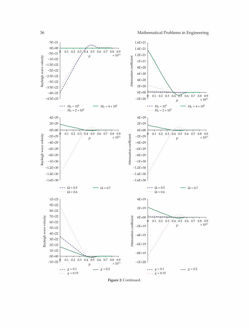
Figure 2 shows the velocity of Rayleigh waves (Re) and attenuation coefficient (Im) underthe effect of gravity field, friction coefficient, magnetic field, relaxation time, and rotationwithrespect to the initial stress; we found that the velocity of Rayleigh waves (Re) and attenuation
Figure 2: Effects of H0,Ω, g, τ1, and p on Rayleigh wave velocity and attenuation coefficient with respectto the initial stress.
coefficient (Im) increased with increasing values of p and H0, and the velocity of Rayleighwaves (Re) and attenuation coefficient (Im) decreased and increased with increasing valuesof g and K, respectively; while the values of (Re) and (Im) take one curve at another value ofthe relaxation time τ1 increased with increasing values of initial stress P .
Figure 3 shows the velocity of Rayleigh waves (Re) and attenuation coefficient (Im)under effect of initial stress, gravity field, friction coefficient, magnetic field, relaxation timeand rotation with respect to the wave number, we find that the velocity of Rayleigh waves(Re) and attenuation coefficient (Im) decreased and increased with increasing values ofH0, respectively, and the velocity of Rayleigh waves (Re) and attenuation coefficient (Im)increased and decreased with increasing values of Ω and g, respectively; also, the values of(Re) and (Im) increased with increasing values of K, while the values of (Re) and (Im) takeone curve at another value of the relaxation time τ1, decreasedwith increasing values of wavenumber k.
Figure 3: Effects of H0,Ω, g, τ1, and K, P on Rayleigh wave velocity and Attenuation coefficient withrespect to the wave number.
6.2. If the Initial Stresses Are Neglected
Figure 4 shows the velocity of Rayleigh waves (Re) and attenuation coefficient (Im) undereffect of gravity field, friction coefficient, magnetic field, relaxation time, and rotation withrespect to the wave number, we find that the velocity of Rayleigh waves (Re) and attenuation
Figure 4: Effects ofH0,Ω, g, τ1, and K on Rayleigh wave velocity and attenuation coefficient with respectto the wave number.
coefficient (Im) decreased with increasing values of H0 and Ω, while that contrary withincreasing values of g; also, the values of (Re) and (Im) increased and decreased withincreasing values of K, respectively, while the values of (Re) and (Im) take one curve atanother value of the relaxation time τ1 decreased, then increased with increasing values ofwave number k.
6.3. If the Initial Stresses and Magnetic Field Are Neglected
Figure 5 shows that the velocity of Rayleigh waves (Re) and attenuation coefficient (Im)under effect of gravity field, friction coefficient, relaxation time, and rotation with respect tothe wave number; we find that the velocity of Rayleighwaves (Re) and attenuation coefficient(Im) decreased and increased with increasing values of Ω, and the values of (Re) and (Im)increasedwith increasing values of g, while that contrarywith increasing values ofK; also, the
Figure 5: Effects of Ω, g, τ1, and K on Rayleigh wave velocity and attenuation coefficient with respect tothe wave number.
values of (Re) and (Im) take one curve at another value of the relaxation time τ1, increased,then decreased with increasing values of wave number k.
6.4. If the Initial Stresses, Magnetic Field, and Gravity Field Are Neglected
Figure 6 shows the velocity of Rayleighwaves (Re) and attenuation coefficient (Im) under theeffect of friction coefficient, relaxation time, and rotation with respect to the wave number;we find that the velocity of Rayleigh waves (Re) and attenuation coefficient (Im) decreasedand increased with increasing Ω, and the values of (Re) and (Im) decreased with increasingvalues ofK, while the values of (Re) and (Im) take one curve at another value of the relaxationtime τ1, decreased and increased with increasing values of the wave number k, respectively.
6.5. If the Initial Stresses, Magnetic Field, and Gravity Field Are Neglectedand There Is Uncoupling between the Temperature and Strain Field
Figure 7 shows the velocity of Rayleighwaves (Re) and attenuation coefficient (Im) under theeffect of friction coefficient, relaxation time, and rotation with respect to the wave number;we find that the velocity of Rayleigh waves (Re) and attenuation coefficient (Im) increasedand decreased with increasing of Ω, respectively, while that contrary with increasing valuesof K; finally, the values of (Re) and (Im) take one curve at another value of the relaxation timeτ1, decreased with increasing, the values of the wave number k.
7. Conclusions
The problem of the Rayleigh waves in generalized magneto-thermo-viscoelastic granularmedium under the influence of rotation, gravity field, and initial stress is considered, andthe frequency equation of the wave motion in the explicit form is derived, by considering
44 Mathematical Problems in Engineering
0 0.05 0.1 0.15 0.2 0.25 0.3 0.35
k ×10−20
0 0.05 0.1 0.15 0.2 0.25 0.3 0.35
k ×10−20
0 0.05 0.1 0.15 0.2 0.25 0.3 0.35
k ×10−20
0 0.05 0.1 0.15 0.2 0.25 0.3 0.35
k ×10−20
0 0.05 0.1 0.15 0.2 0.25 0.3 0.35
k ×10−20
0 0.05 0.1 0.15 0.2 0.25 0.3 0.35
k ×10−20
Ω = 0.5Ω = 0.6
Ω = 0.7
τ1 = 0.3τ1 = 0.4
τ1 = 0.5
K = 0.1K = 0.2
K = 0.3
Ω = 0.5Ω = 0.6
Ω = 0.7
τ1 = 0.3τ1 = 0.4
τ1 = 0.5
K = 0.1K = 0.2
K = 0.3
−3.5E+55
−3E+55
−2.5E+55
−2E+55
−1.5E+55
−1E+55
−5E+54
0E+00
5E+54
−5E+55
−4E+55
−3E+55
−2E+55
−1E+55
0E+00
1E+55
−2E+18
0E+00
2E+18
4E+18
6E+18
8E+18
1E+19
1.2E+19
1.4E+19
1.6E+19
−5E+18
−4E+18
−3E+18
−2E+18
−1E+18
0E+00
1E+18
−1.6E+26
−1.4E+26
−1.2E+26
−1E+26
−8E+25
−6E+25
−4E+25
−2E+250E+00
2E+25
−5E+23
0E+00
5E+23
1E+24
1.5E+24
2E+24
2.5E+24
Ray
leighwav
eve
locity
Ray
leighwav
eve
locity
Ray
leighwav
eve
locity
Atten
uation
coeffi
cien
tAtten
uation
coeffi
cien
tAtten
uation
coeffi
cien
t
Figure 6: Effects of Ω, τ1, and K on Rayleigh wave velocity and attenuation coefficient with respect to thewave number.
Mathematical Problems in Engineering 45
−1E+285
0E+00
0E+00
1E+285
2E+285
3E+285
4E+285
5E+285
−1.6E+288
−1.4E+288
−1.2E+288
−1E+288
−8E + 287
−6E+287
−4E+287
2E+287
−2E+287
−5E+280
0E+000E+00
5E+280
1E+281
1.5E+281
2E+281
2.5E+281
−5E+283
5E+283
1E+284
1.5E+284
2E+284
2.5E+284
3E+284
3.5E+284
4E+284
−3E+304
−2.5E+304
−2E+304
−1.5E+304
−1E+304
−5E+303
0E+00
5E+303
−2E+301
0E+00
2E+301
4E+301
6E+301
8E+301
1E+302
1.2E+302
1.4E+302
Ray
leighwav
eve
locity
Ray
leighwav
eve
locity
Ray
leighwav
eve
locity
Atten
uation
coeffi
cien
tAtten
uation
coeffi
cien
tAtten
uation
coeffi
cien
t
0 0.05 0.1 0.15 0.2 0.25 0.3 0.35
k ×10−20
0 0.05 0.1 0.15 0.2 0.25 0.3 0.35
k ×10−20
0 0.05 0.1 0.15 0.2 0.25 0.3 0.35
k ×10−20
0 0.05 0.1 0.15 0.2 0.25 0.3 0.35
k ×10−20
0 0.05 0.1 0.15 0.2 0.25 0.3 0.35
k ×10−20
0 0.05 0.1 0.15 0.2 0.25 0.3 0.35
k ×10−20
Ω = 0.5Ω = 0.6
Ω = 0.7 Ω = 0.5Ω = 0.6
Ω = 0.7
τ1 = 0.3τ1 = 0.4
τ1 = 0.5 τ1 = 0.3τ1 = 0.4
τ1 = 0.5
K = 0.1K = 0.2
K = 0.3 K = 0.1K = 0.2
K = 0.3
Figure 7: Effects of Ω, τ1, and K on Rayleigh wave velocity and attenuation coefficient with respect to thewave number.
46 Mathematical Problems in Engineering
various special cases. The numerical results are obtained for carbon-steel material, althoughthe effect of the rotation, magnetic field, relaxation times, initial stress, gravity field, andfriction coefficient is observed to be quite large on wave propagation of Rayleigh wavevelocity (Re) and attenuation coefficient (Im).
The problem of the Rayleigh waves in generalized magneto-thermo-viscoelasticgranularmediumunder the influence of rotation, gravity field, and initial stress is considered,and the frequency equation of the wavemotion in the explicit form is derived, by consideringvarious special cases. The numerical results are obtained for carbon-steel material, althoughthe effect of the rotation, magnetic field, relaxation times, initial stress, gravity field, andfriction coefficient is observed to be quite large on wave propagation of Rayleigh wavevelocity (Re) and attenuation coefficient (Im).
It is easy to see that the values of (Re) and (Im) with respect to the initial stress areincreased with increasing values of Ω, while that contrary if the initial stress are neglectedand with respect to the wave number; also, if the initial stress are constant with respect to thewave number the values of (Re) and (Im) increased and decreased with increasing valuesof Ω, respectively, and if the initial stress and the magnetic field are neglected, the values of(Re) and (Im) decreased and increased with increasing values of Ω, respectively, while thatcontrary if P,H0, g, θ, and ε are neglected and with respect to the wave number; finally, ifP,H0, and g are neglected and with respect to the wave number, the values of (Re) and (Im)increased with increasing values of Ω.
It is easy to see that the values of (Re) and (Im) with respect to the initial stress aredecreased and increased with increasing values of g, respectively, while that contrary if theinitial stress are constant and with respect to the wave number; also, if the initial stress areneglected and if the initial stress and the magnetic field are neglected with respect to the wavenumber, the values of (Re) and (Im) increased with increasing values of g.
It is easy to see that the values of (Re) and (Im) with respect to the initial stressare decreased and increased with increasing values of K, respectively, while that contraryif the initial stress are neglected and with respect to the wave number; also, if the initialstress and the magnetic field are neglected and if P,H0, and g are neglected with respect thewave number, the values of (Re) and (Im) decreased with increasing values of K; finally, ifP,H0, g, θ, and ε are neglected and with respect to the wave number, the values of (Re) and(Im) decreased and increased with increasing values of K.
Finally, the frequency equation has been discussed under effect of rotation, gravityfield, and initial stress and in case of various classical and nonclassical theories ofthermoelasticity. The results indicate that the effect of rotation, magnetic field, initial stress,and gravity field is very pronounced. The frequency equations derived in this paper maybe useful in practical applications. It is concluded from the above analyses and results thatthe present solution is accurate and reliable and the method is simple and effective. So itmay be as a reference to solve other problems of Rayleigh waves in generalized magneto-thermoelastic granular medium.
References
[1] N. Oshima, “A symmetrical stress tensor and its application to a granular medium,” in Proceedings ofthe 3 rd Japan National congress for Applied Mechanics, vol. 77, pp. 77–83, 1955.
[2] A.M. El-Naggar, “On the dynamical problemof a generalized thermoelastic granular infinite cylinderunder initial stress,”Astrophysics and Space Science, vol. 190, no. 2, pp. 177–190, 1992.
Mathematical Problems in Engineering 47
[3] N. C. Dawan and S. K. Chakraporty, “On Rayleigh waves in Green-Lindsay model of generalizedthermoelastic media,” Indian Journal Pure and Applied Mathematics, vol. 20, pp. 276–283, 1998.
[4] A. M. Abd-Alla, H. A. H. Hammad, and S. M. Abo-Dahab, “Rayleigh waves in a magnetoelastic half-space of orthotropic material under influences of initial stress and gravity field,” Applied Mathematicsand Computation, vol. 154, no. 2, pp. 583–597, 2004.
[5] A. M. El-Naggar, A. M. Abd-Alla, and S. M. Ahmed, “Rayleigh waves in a magnetoelastic initiallystressed conducting medium with the gravity field,” Bulletin of the Calcutta Mathematical Society, vol.86, no. 3, pp. 243–248, 1994.
[6] S. M. Ahmed, “Rayleigh waves in a thermoelastic granular medium under initial stress,” InternationalJournal of Mathematics and Mathematical Sciences, vol. 23, no. 9, pp. 627–637, 2000.
[7] A. M. Abd-Alla and S. M. Ahmed, “Rayleigh waves in an orthotropic thermoelastic medium undergravity and initial stress,” Earth, Moon and Planets, vol. 75, pp. 185–197, 1998.
[8] A. M. Abd-Alla and S. R. Mahmoud, “Magneto-thermoelastic problem in rotating non-homogeneousorthotropic hollow cylinder under the hyperbolic heat conduction model,” Meccanica, vol. 45, no. 4,pp. 451–462, 2010.
[9] M. Venkatesan and P. Ponnusamy, “Wave propagation in a generalized thermoelastic solid cylinderof arbitrary cross-section immersed in a fluid,” International Journal of Mechanical Sciences, vol. 49, no.6, pp. 741–751, 2007.
[10] S. K. Roychoudhuri and N. Bandyopadhyay, “Thermoelastic wave propagation in a rotating elasticmedium without energy dissipation,” International Journal of Mathematics and Mathematical Sciences,no. 1, pp. 99–107, 2005.
[11] J. N. Sharma and D. Grover, “Body wave propagation in rotating thermoelastic media,” MechanicsResearch Communications, vol. 36, no. 6, pp. 715–721, 2009.
[12] A. M. El-Naggar, A. M. Abd-Alla, M. A. Fahmy, and S. M. Ahmed, “Thermal stresses in a rotatingnon-homogeneous orthotropic hollow cylinder,”Heat and Mass Transfer, vol. 39, no. 1, pp. 41–46, 2002.
[13] M. R. Abd-El-Salam, A. M. Abd-Alla, and H. A. Hosham, “A numerical solution of magneto-thermoelastic problem in non-homogeneous isotropic cylinder by the finite-difference method,”Applied Mathematical Modelling, vol. 31, no. 8, pp. 1662–1670, 2007.
[14] S. Mukhopadhyay, “Effects of thermal relaxations on thermoviscoelastic interactions in anunbounded body with a spherical cavity subjected to a periodic loading on the boundary,” Journalof Thermal Stresses, vol. 23, no. 7, pp. 675–684, 2000.
[15] A. M. Abd-Alla, “Propagation of Rayleigh waves in an elastic half-space of orthotropic material,”Applied Mathematics and Computation, vol. 99, no. 1, pp. 61–69, 1999.
[16] Masa. Tanaka, T. Matsumoto, and M. Moradi, “Application of boundary element method to 3-Dproblems of coupled thermoelasticity,” Engineering Analysis with Boundary Elements, vol. 16, no. 4,pp. 297–303, 1995.
[17] W. Nowacki, Thermoelasticity, Addison-Wesley, London, UK, 1962.[18] M. A. Biot, Mechanics of Incremental Deformations. Theory of Elasticity and Viscoelasticity of Initially
Stressed Solids and Fluids, Including Thermodynamic Foundations and Applications to Finite Strain, JohnWiley & Sons, New York, NY, USA, 1965.
[19] P. M. Morse and H. Feshbach, Methods of Theoretical Physics, McGraw-Hill, New York, NY, USA, 1953.[20] A. M. Abd-Alla, S. M. Abo-Dahab, H. A. Hammad, and S. R. Mahmoud, “On generalized magneto-
thermoelastic rayleigh waves in a granular medium under the influence of a gravity field and initialstress,” Journal of Vibration and Control, vol. 17, no. 1, pp. 115–128, 2011.
[21] J. N. Sharma and M. Pal, “Rayleigh-Lamb waves in magneto-thermoelastic homogeneous isotropicplate,” International Journal of Engineering Science, vol. 42, no. 2, pp. 137–155, 2004.