Development of Simple Performance Tests Using Laboratory Test Procedures to Illustrate the Effects of Moisture Damage on Hot Mix Asphalt Jason Bausano 1 Andrea Kvasnak 1 R. Christopher Williams 1 , Ph.D. Final Report
Transcript
Development of Simple Performance Tests Using Laboratory Test Procedures to Illustrate the Effects of Moisture Damage on Hot Mix Asphalt Jason Bausano1
Andrea Kvasnak1
R. Christopher Williams1, Ph.D.
Final Report
ii
DISCLAIMER
This document is disseminated under the sponsorship of the Federal Highway
Administration (FHWA) in the interest of information exchange. FHWA assumes no
liability for its content or use thereof.
The contents of this report reflect the views of the contracting organization, which is
responsible for the accuracy of the information presented herein. The contents may not
necessarily reflect the views of FHWA and do not constitute standards, specifications, or
regulations.
iii
1. Report No. RC-1521 2. Government
Accession No.
3. Recipient’s Catalog No.
4. Title and Subtitle
Development of Simple Performance Tests Using
Laboratory Test Procedures to Illustrate the Effects of
Moisture Damage on Hot Mix Asphalt
5. Report Date
April 5, 2006
7. Author(s)
Jason Bausano, Andrea Kvasnak, & R. Christopher
Williams, Ph.D.
6. Performing Organization Code
9. Performing Organization Name and Address
Michigan Technological University
Department of Civil and Environmental Engineering
1400 Townsend Drive
Houghton, MI 49931
8. Performing Org Report No.
12. Sponsoring Agency Name and Address
Federal Highway Administration
10. Work Unit No. (TRAIS)
11. Contract/Grant No. DTFH61-02-C-
00074
11a. 00-MTU-5
15. Supplementary Notes 13. Type of Report and Period Covered
Final Report
14. Sponsoring Agency Code
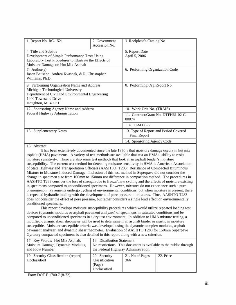
16. Abstract
It has been extensively documented since the late 1970’s that moisture damage occurs in hot mix
asphalt (HMA) pavements. A variety of test methods are available that test an HMAs’ ability to resist
moisture sensitivity. There are also some test methods that look at an asphalt binder’s moisture
susceptibility. The current test method for detecting moisture sensitivity in HMA is American Association
of State Highway and Transportation Officials (AASHTO) T283: Resistance of Compacted Bituminous
Mixture to Moisture-Induced Damage. Inclusion of this test method in Superpave did not consider the
change in specimen size from 100mm to 150mm nor difference in compaction method. The procedures in
AASHTO T283 consider the loss of strength due to freeze/thaw cycling and the effects of moisture existing
in specimens compared to unconditioned specimens. However, mixtures do not experience such a pure
phenomenon. Pavements undergo cycling of environmental conditions, but when moisture is present, there
is repeated hydraulic loading with the development of pore pressure in mixtures. Thus, AASHTO T283
does not consider the effect of pore pressure, but rather considers a single load effect on environmentally
conditioned specimens.
This report develops moisture susceptibility procedures which would utilize repeated loading test
devices (dynamic modulus or asphalt pavement analyzer) of specimens in saturated conditions and be
compared to unconditioned specimens in a dry test environment. In addition to HMA mixture testing, a
modified dynamic shear rheometer will be used to determine if an asphalt binder or mastic is moisture
susceptible. Moisture susceptible criteria was developed using the dynamic complex modulus, asphalt
pavement analyzer, and dynamic shear rheometer. Evaluation of AASHTO T283 for 150mm Superpave
Gyrtaory compacted specimens is also detailed in this report along with a new criterion.
17. Key Words: Hot Mix Asphalt,
Moisture Damage, Dynamic Modulus,
and Flow Number
18. Distribution Statement
No restrictions. This document is available to the public through
1.1 Moisture Susceptibility ..................................................................................... 10 1.2 Project Objectives ............................................................................................. 11 1.3 Current State of the Practice for Moisture Testing ........................................... 11 1.4 Overall Project Experimental Plan.................................................................... 13 1.5 Hypotheses for Testing Results ........................................................................ 13 1.6 Contents of this Document................................................................................ 13
CHAPTER 2 Literature Review...................................................................................15 2.1 Introduction....................................................................................................... 15 2.2 Causes of Moisture Damage ............................................................................. 15
2.5.1 Tests on Loose Mixture and Asphalt Binders........................................... 20 2.5.1.1 Methylene Blue Test ............................................................................. 21 2.5.1.2 Static Immersion Test (AASHTO T182).............................................. 21 2.5.1.3 Film Stripping Test (California Test 302) ............................................ 22 2.5.1.4 Dynamic Immersion Test...................................................................... 22 2.5.1.5 Chemical Immersion Test ..................................................................... 22 2.5.1.6 Surface Reaction Test ........................................................................... 23 2.5.1.7 Boiling Water Test................................................................................ 23 2.5.1.8 Rolling Bottle Test................................................................................ 23 2.5.1.9 Net Adsorption Test.............................................................................. 24 2.5.1.10 Wilhelmy Plate Test and Universal Sorption Device ....................... 24 2.5.1.11 Pneumatic Pull-Off Test ................................................................... 25 2.5.1.12 Dynamic Shear Rheometer ............................................................... 26
2.5.2 Tests on Compacted Mixtures .................................................................. 26 2.5.2.1 Immersion-Compression Test............................................................... 27 2.5.2.2 Marshall Immersion Test ...................................................................... 28 2.5.2.3 Moisture Vapor Susceptibility .............................................................. 28 2.5.2.4 Repeated Pore Water Pressure Stressing and Double-Punch Method .. 28 2.5.2.5 Original Lottman Method ..................................................................... 29 2.5.2.6 Modified Lottman Test (AASHTO T283)............................................ 29 2.5.2.7 ASTM D4867 (Tunnicliff-Root Test Procedure) ................................. 30
v
2.5.2.8 Texas Freeze/Thaw Pedestal Test......................................................... 31 2.5.2.9 Hamburg Wheel-Tracking Device (HWTD) ........................................ 31 2.5.2.10 Asphalt Pavement Analyzer.............................................................. 32 2.5.2.11 Environmental Conditioning System (ECS)..................................... 33 2.5.2.12 Flexural Fatigue Beam Test with Moisture Conditioning ................ 34 2.5.2.13 ECS/Simple Performance Test Procedures....................................... 34
3.1.1 Phase I Testing – Sensitivity Study .......................................................... 40 3.1.2 Phase I – Preliminary Binder Study.......................................................... 41
3.1.2.1 Gap Size and Interface Selection .......................................................... 42 3.1.3 Phase II Testing......................................................................................... 44
CHAPTER 4 Procedures and Sample Preparation.......................................................48 4.1 Materials Collection.......................................................................................... 48
4.1.1 Splitting..................................................................................................... 48 4.1.2 Maximum Theoretical Specific Gravity (Gmm)......................................... 49
4.3 Compaction of Gyratory and Marshall Specimens........................................... 58 4.3.1 Bulk Specific Gravity (Gmb) ..................................................................... 60
4.4 Bulk Specific Gravity of Gyratory and Marshall Specimens ........................... 61 4.4.1 Specimen Cutting and Coring................................................................... 61
4.5 Specimen Measurement .................................................................................... 62 4.6 Volumetrics of Sawed/Cored Test Specimens.................................................. 62 4.7 Testing and Calculations................................................................................... 63
CHAPTER 6 sensitivity Study – Evaluation of AASHTO T283 ................................84 6.1 Introduction....................................................................................................... 84 6.2 AASHTO T283 Test Results ............................................................................ 84 6.3 Analysis of Results ........................................................................................... 94
vi
6.4 Conclusions....................................................................................................... 99 CHAPTER 7 Preliminary binder study test results....................................................101
7.1 Introduction..................................................................................................... 101 7.2 Gap Size and Interface Selection .................................................................... 101 7.3 Saturation Effects on Asphalt Binders............................................................ 104 7.4 Delay Effects on Asphalt Binders................................................................... 106 7.5 AAA-1 and AAM-1 DSR Testing Conclusions ............................................. 106
CHAPTER 8 Testing of Michigan Mixes for Moisture Damage – Phase II .............108 8.1 Introduction..................................................................................................... 108 8.2 Experimental Plan........................................................................................... 108 8.3 AASHTO T283 Test Results .......................................................................... 110 8.4 Dynamic Modulus Test Results ...................................................................... 112 8.5 DSR Test Results ............................................................................................ 121
8.5.1 Materials for Field Binder Testing.......................................................... 122 8.5.2 Statistical and Graphical Results of Michigan Binder Tests .................. 125 8.5.3 Statistical and Graphical Comparisons of All Michigan Binders........... 125
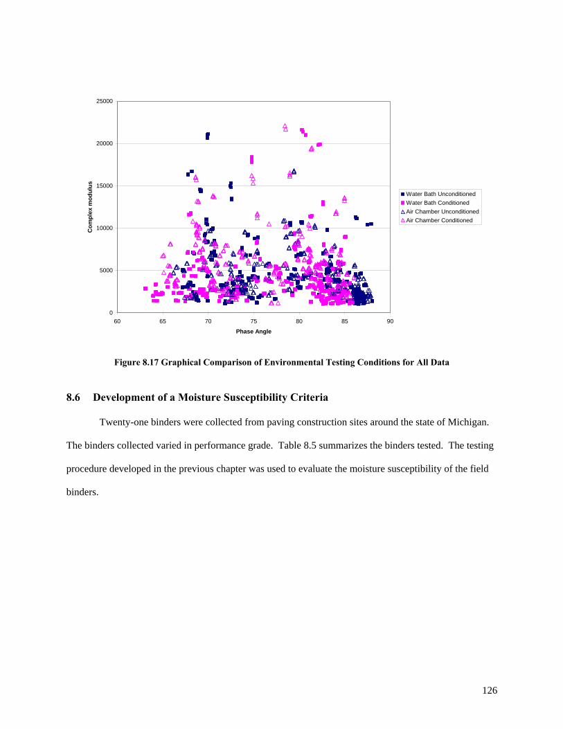
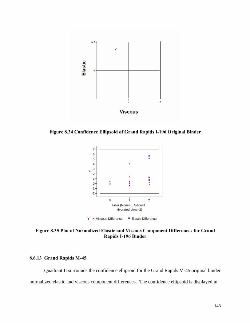
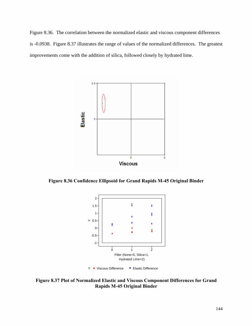
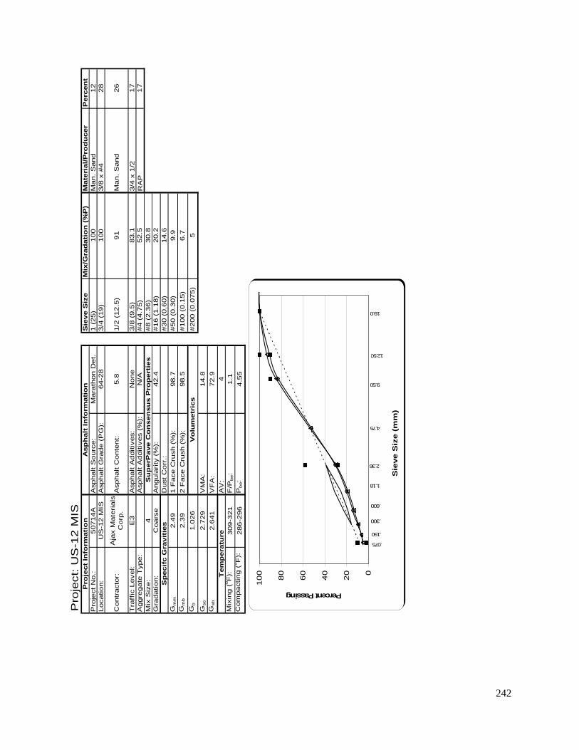
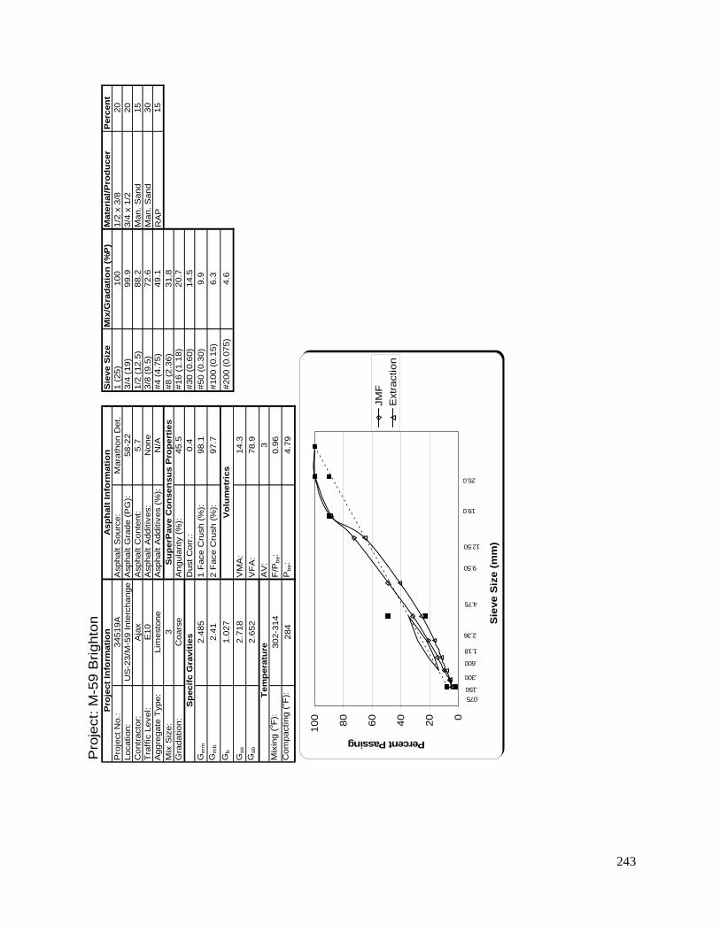
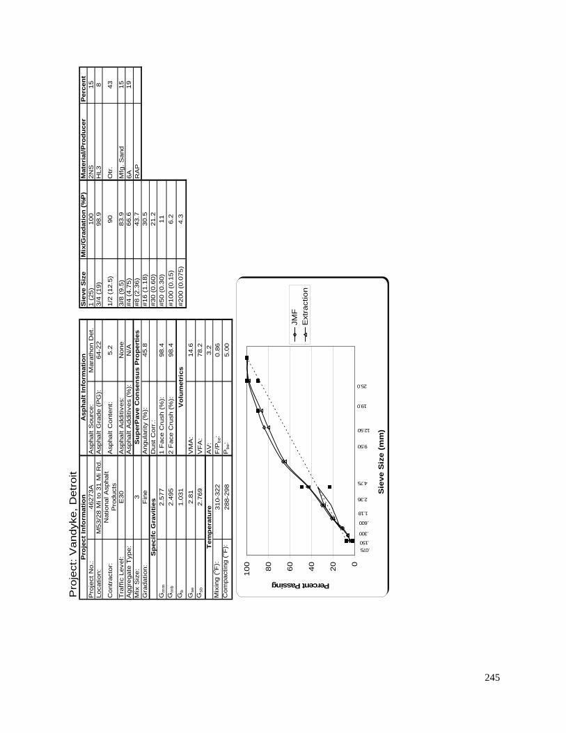
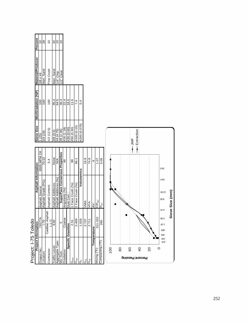
8.6 Development of a Moisture Susceptibility Criteria ........................................ 126 8.6.1 Hypotheses.............................................................................................. 127 8.6.2 Asphalt Binder Criteria ........................................................................... 128 8.6.3 Application of Superpave Asphalt Binder Criterion............................... 129 8.6.4 Viscous and Elastic Component Analysis .............................................. 129 8.6.5 I-94 Ann Arbor ....................................................................................... 132 8.6.6 M-66 Battle Creek................................................................................... 134 8.6.7 M-59 Brighton ........................................................................................ 135 8.6.8 I-75 Clarkston ......................................................................................... 136 8.6.9 M-53 Detroit ........................................................................................... 138 8.6.10 M-50Dundee 19.0mm NMAS ................................................................ 139 8.6.11 M-50Dundee 125mm NMAS ................................................................. 141 8.6.12 Grand Rapids I-196................................................................................. 142 8.6.13 Grand Rapids M-45................................................................................. 143 8.6.14 US-23 Hartland ....................................................................................... 145 8.6.15 BL I-96 Howell ....................................................................................... 146 8.6.16 I-75 Levering Road ................................................................................. 147 8.6.17 Michigan Ave 19.0mm NMAS............................................................... 149 8.6.18 Michigan Ave 12.5mm NMAS............................................................... 150 8.6.19 Michigan International Speedway US-12............................................... 151 8.6.20 M-21 Owosso.......................................................................................... 152 8.6.21 M-36 Pinckney........................................................................................ 154 8.6.22 M-84 Saginaw......................................................................................... 155 8.6.23 M-21 St. Johns ........................................................................................ 156 8.6.24 I-75 Toledo.............................................................................................. 157 8.6.25 Van Dyke, Detroit ................................................................................... 158 8.6.26 Summary of Statistical Noise.................................................................. 159 8.6.27 Summary of Correlation of Normalized Component Differences.......... 160
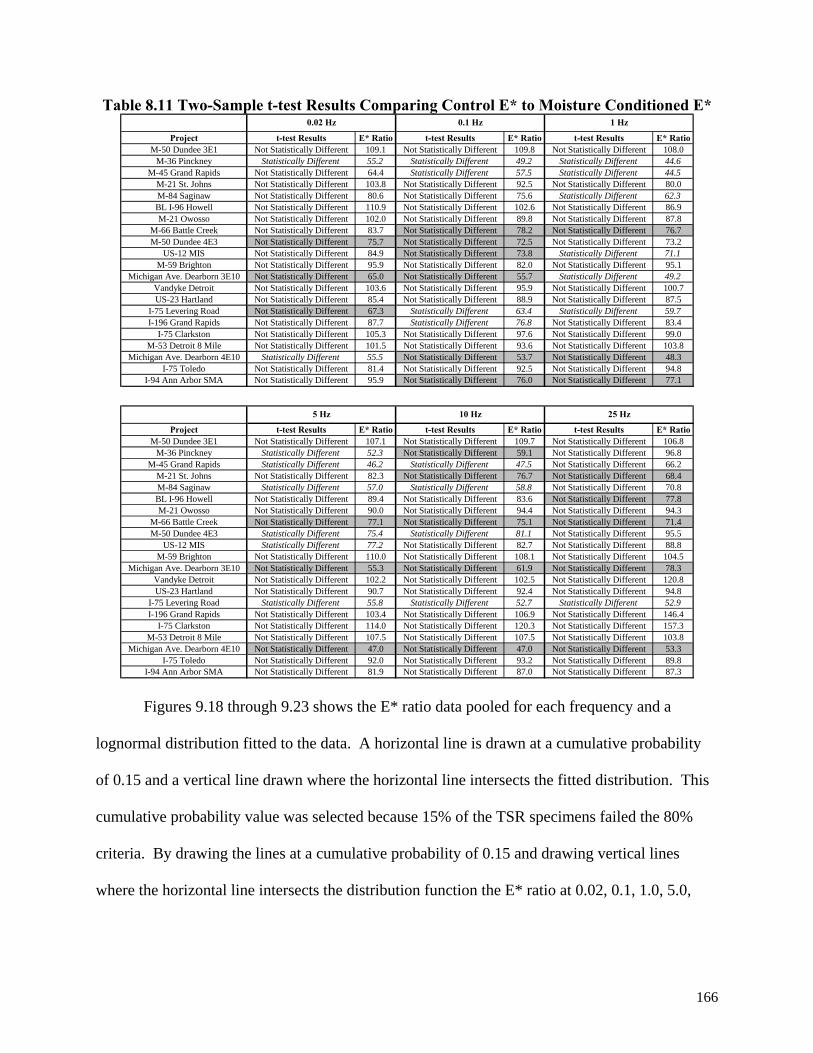
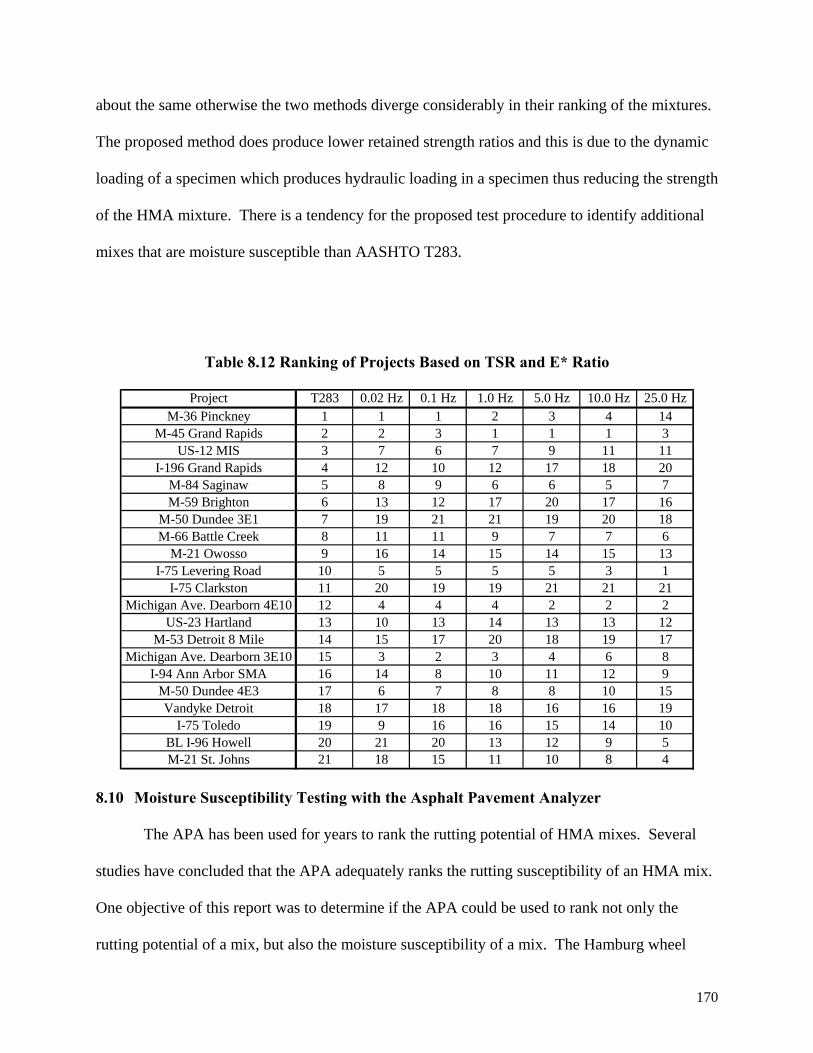
8.9 Analysis of Results – E* Ratio ....................................................................... 165 8.10 Moisture Susceptibility Testing with the Asphalt Pavement Analyzer .......... 170
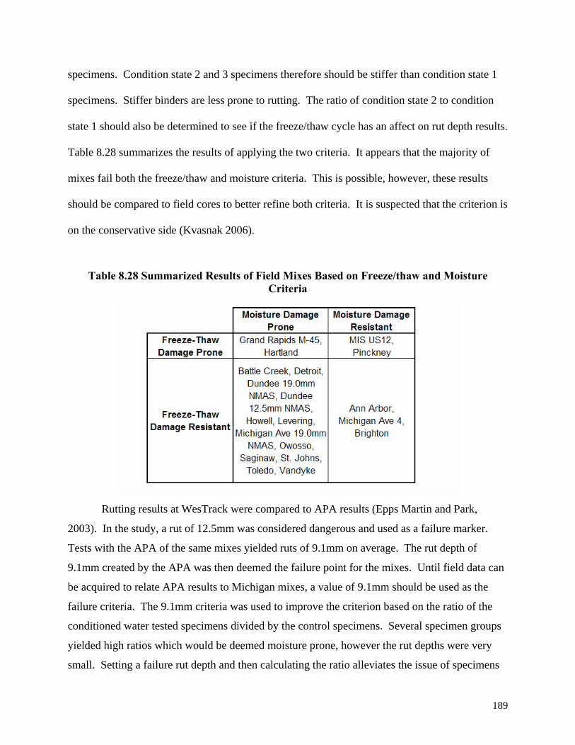
8.10.1 Sensitivity Study ..................................................................................... 171 8.10.2 APA Testing of Field Sampled HMA..................................................... 172 8.10.3 Conditioning of the HMA Specimens for APA Testing......................... 172 8.10.4 APA Test Results for Field Sampled HMA............................................ 174 8.10.5 Analysis of All APA Data....................................................................... 174 8.10.6 General Linear Model Analysis of APA Data ........................................ 178 8.10.7 APA Analysis Summary ......................................................................... 188 8.10.8 APA Moisture Criteria............................................................................ 188 8.10.9 Summary of Phase I TSR and APA Comparison ................................... 192 8.10.10 Comparison of Moisture Susceptibility Testing of HMA Mixes and Asphalt Binders 192 8.10.11 APA Conclusions................................................................................ 193
8.11 Analysis of Results – DSR.............................................................................. 194 8.11.1 Statistical and Graphical Results of Michigan Binders Categorized by Mastic Type 198
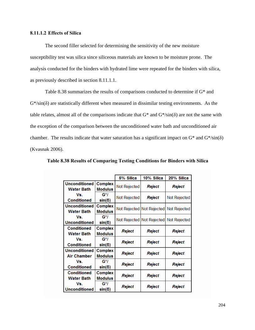
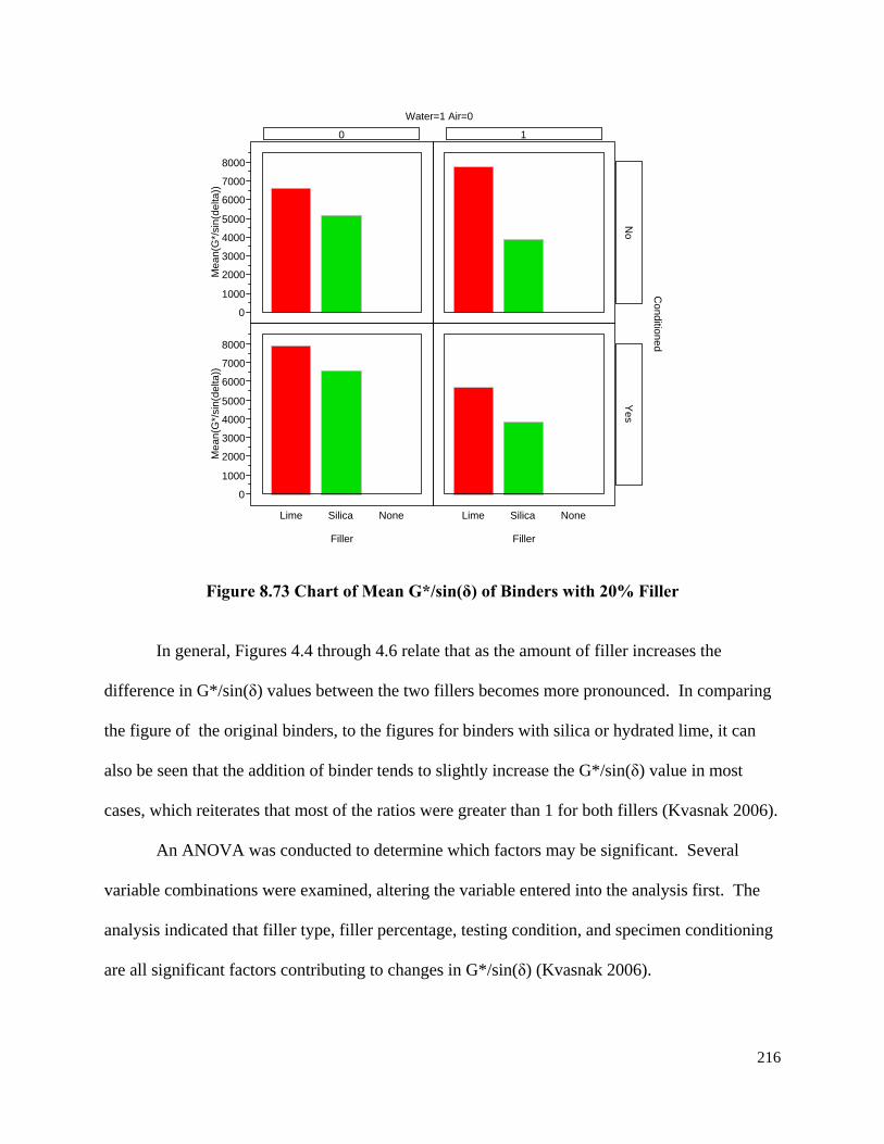
8.11.1.1 Effects of Hydrated Lime................................................................ 199 8.11.1.2 Effects of Silica............................................................................... 204 8.11.1.3 Comparison of Hydrated Lime to Silica ......................................... 211
8.11.2 Conclusions about Filler Effects............................................................. 217 8.12 Moisture Damage Factors Affecting TSR and E* Values .............................. 217
9.2.1 AASHTO T283 – Phase I ....................................................................... 226 9.2.2 Moisture Testing – Phase II .................................................................... 227
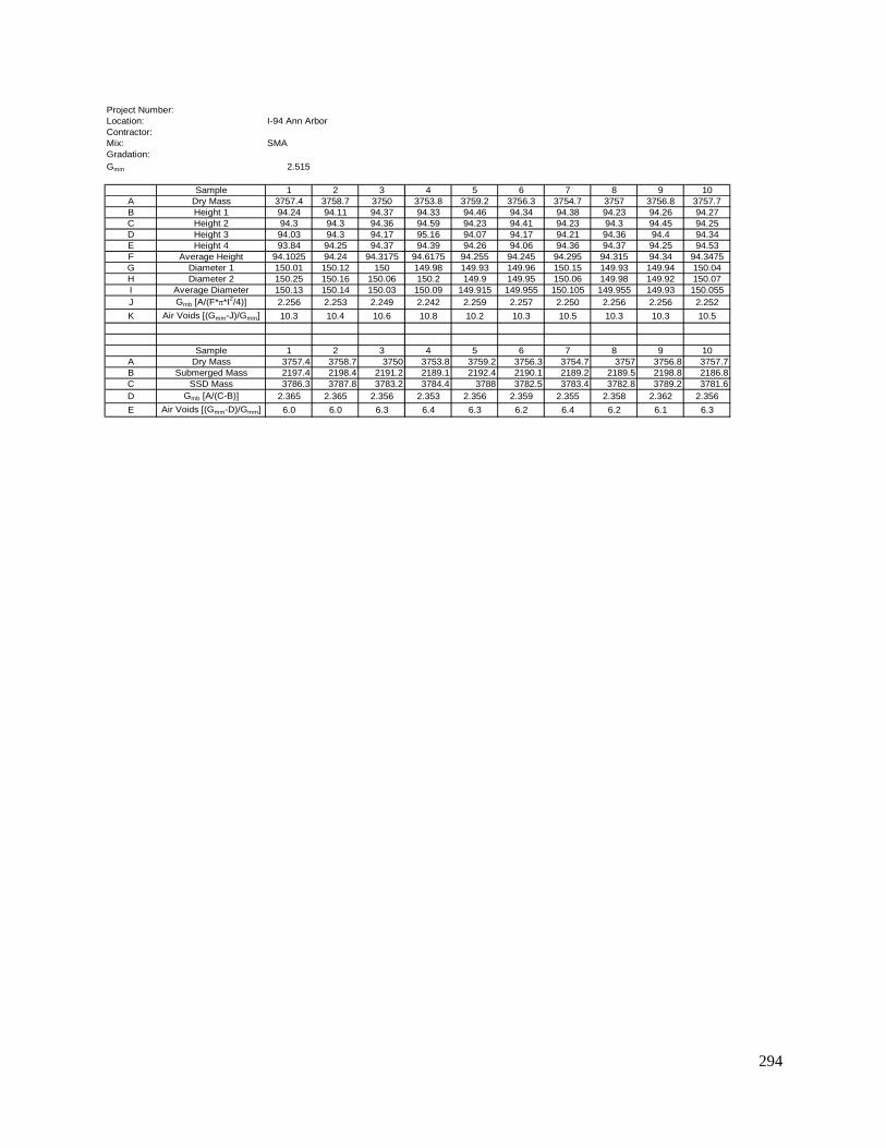
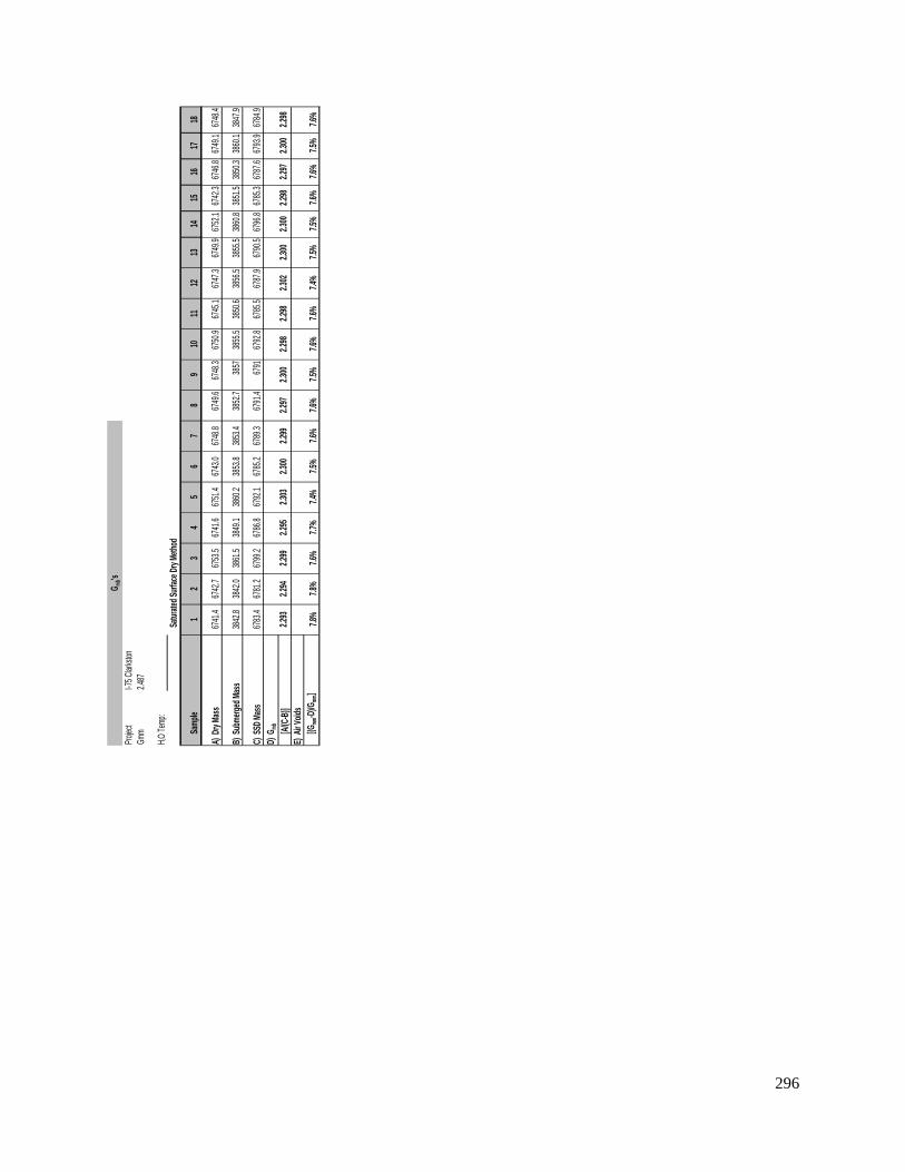
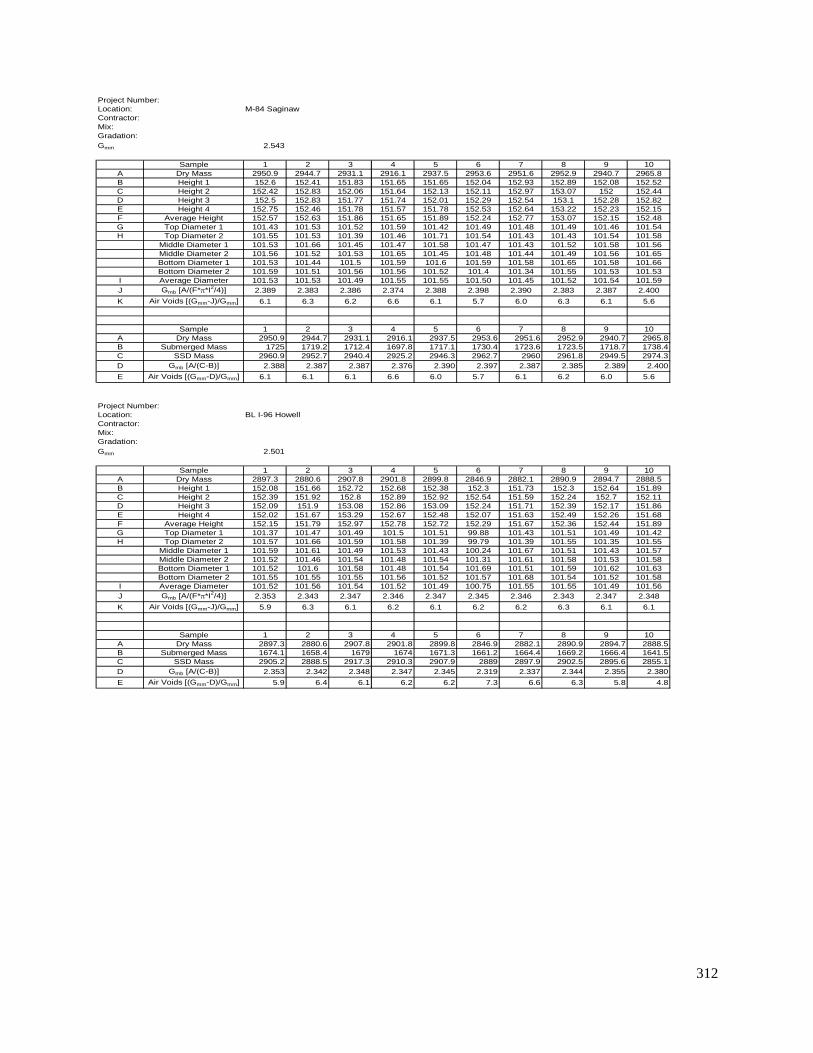
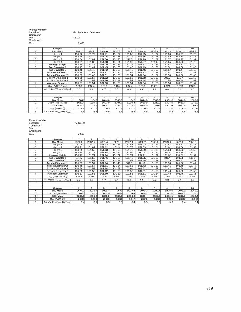
9.3 Recommendations........................................................................................... 230 APPENDIX A JOB MIX FORUMALA’S……………………………………………...205 APPENDIX B SPECIMEN VOLUMETRICS………………………………………….227 APPENDIX C SAS OUTPUTS…………...…………………………………………….294 REFERENCES…………………………………………………………………………...350
viii
LIST OF TABLES
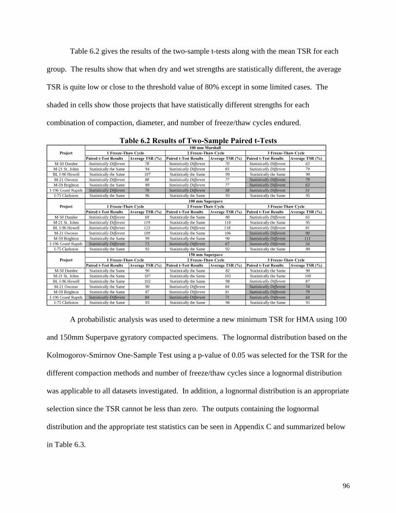
Table 2.1 Moisture Sensitivity Tests on Loose Samples (Solaimanian et al. 2003)......... 20 Table 2.2 Moisture Sensitivity Tests on Compacted Samples.......................................... 27 Table 2.3 SPT Advantages and Disadvantages (Witczak et al. 2002 and ........................ 36 Table 3.1 Sensitivity Study Experimental Plan for Mix and Aggregate Types................ 40 Table 3.2 Sensitivity Study Experimental Plan for Effect of Compaction Method and Conditioning Period on Performance................................................................................ 41 Table 3.3 Properties of Ceramic Discs (Rottermond, 2004)............................................. 42 Table 3.4 Gap Size and Interface Selection Experimental Plan ....................................... 43 Table 3.5 Experimental Plan for AAA-1 and AAM-1 Asphalt Binders........................... 44 Table 3.6 Laboratory Experimental Plan for Phase II ...................................................... 44 Table 4.1 Gmm Mean and Standard Deviation for Each Project........................................ 50 Table 4.2 2-Way ANOVA Comparing Laboratory Gmm to Contractor JMF.................... 52 Table 4.3 Extracted Binder Content versus JMF Binder Content .................................... 54 Table 4.4 2-Way ANOVA Comparing Laboratory Extracted Binder Content to ............ 56 Table 4.5 2-Way ANOVA Comparing Laboratory Extracted Gradation to JMF Gradation57 Table 4.6 Dynamic Modulus Testing Configurations....................................................... 66 Table 4.7 Cycles for Test Sequence.................................................................................. 66 Table 5.1 Rutting Effective Test Temperatures................................................................ 80 Table 5.2 Fatigue Effective Test Temperatures................................................................ 81 Table 5.3 APA Test Temperatures.................................................................................... 83 Table 6.1 Ranking of Projects Based on TSR................................................................... 93 Table 6.2 Results of Two-Sample Paired t-Tests.............................................................. 96 Table 6.3 Goodness of Fit Statistics for Phase I Distributions ......................................... 97 Table 7.1 Repeatability of 200μm and 300μm Gap Size................................................ 102
ix
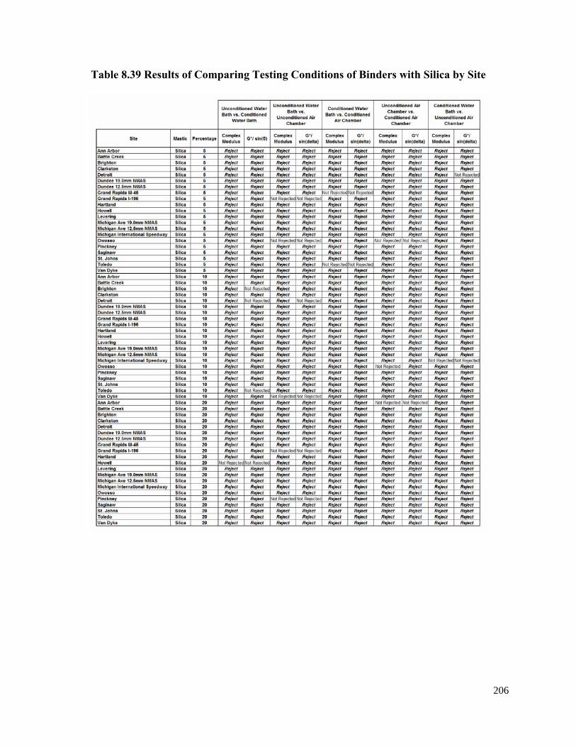
Table 7.2 P-Values of Main and Interaction Effects on Complex Shear Modulus Results104 Table 7.3 P-Values of Condition Comparisons of Original Binders .............................. 105 Table 7.4 P-Values Comparing Delay Times ................................................................. 106 Table 8.1 Expanded Experimental Plan for Phase II Projects ........................................ 109 Table 8.2 Laboratory Experimental Plan for Phase II .................................................... 110 Table 8.3 Samples Tested ............................................................................................... 124 8.4 Testing Plan for Each Michigan Binder.................................................................... 125 Table 8.5 Summary of Binders Tested ........................................................................... 127 Table 8.6 Normalized Viscous and Component of Original Binders Standard Deviation Analysis Summary ......................................................................................................................... 132 Table 8.7 Location of Confidence Ellipsoids ................................................................. 160 Table 8.8 Correlation Ratings of Normalized Viscous and Elastic Component Differences161 Table 8.9 Goodness of Fit Statistics for Phase II............................................................ 163 Table 8.10 Two-Sample t-test Results Comparing Dry Strength to Wet Strength......... 164 Table 8.11 Two-Sample t-test Results Comparing Control E* to Moisture Conditioned E* 166 Table 8.12 Ranking of Projects Based on TSR and E* Ratio......................................... 170 Table 8.13 Mean Comparison by Condition State.......................................................... 175 Table 8.14 Mean Comparison by PG High Temperature ............................................... 175 Table 8.15 Mean Comparisons by Test Temperature..................................................... 176 Table 8.16 Mean Comparisons by NMAS...................................................................... 176 Table 8.17 Mean Comparisons by ESAL Level ............................................................. 176 Table 8.18 Mean Comparisons by Gradation ................................................................. 177 Table 8.19 Summary of Rut Depth Mean Comparison .................................................. 177 Table 8.20 Summary of ANOVA for All of the APA data ............................................ 179 Table 8.21 Regression Parameter Estimated for All APA Data ..................................... 181 Table 8.22 Summary of ANOVA for Condition State 1 APA Data............................... 182 Table 8.23 Regression Parameter Estimates for Condition State 1 APA Rut Depth Data183 Table 8.24 Summary of ANOVA for Condition State 2 APA Rut Depth Data ............. 184 Table 8.25 Regression Parameter Estimates for Condition State 2 APA Rut Depth Data185 Table 8.26 Summary of ANOVA for Condition State 3 APA Rut Depth Data ............. 186 Table 8.27 Regresion Parameter Estimates for Condition State 3 APA Rut Depth Data187 Table 8.28 Summarized Results of Field Mixes Based on Freeze/thaw and Moisture Criteria......................................................................................................................................... 189 Table 8.29 Summary of Rut Depth Failure for all Three Condition States .................... 191 Table 8.30 Rut Depth Ratios of Mixes that Failed the Rut Depth Maximum Criterion. 191 Table 8.31 Moisture Susceptible Comparison ................................................................ 193 Table 8.32 Comparison of Testing Conditions for All Data........................................... 196 Table 8.34 Results of Comparing Environmental Testing Conditions by Mastic Percentage Level......................................................................................................................................... 199 Table 8.35 Results of Hydrated Lime Comparisons Grouped by Percentage of Filler .. 200 Table 8.36 Results of Hydrated Lime Comparing Testing Conditions .......................... 202 Table 8.37 Ratio G*/sin(δ) of Hydrated Lime to Original Binder.................................. 203 Table 8.38 Results of Comparing Testing Conditions for Binders with Silica .............. 204 Table 8.39 Results of Comparing Testing Conditions of Binders with Silica by Site.... 206 Table 8.40 G*/sin(δ) Ratio of Silica to Original Binder................................................. 207 Table 8.41 Ratio of G*/sin(δ) Conditioned to Unconditioned Specimens ..................... 209
x
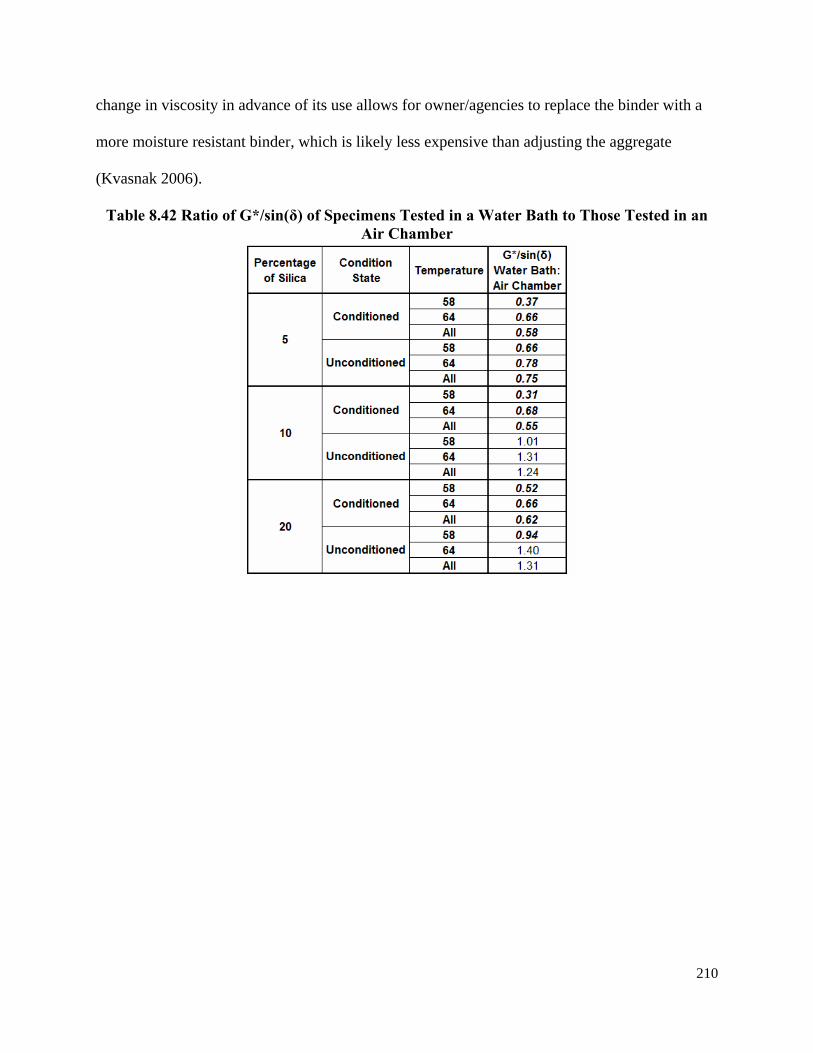
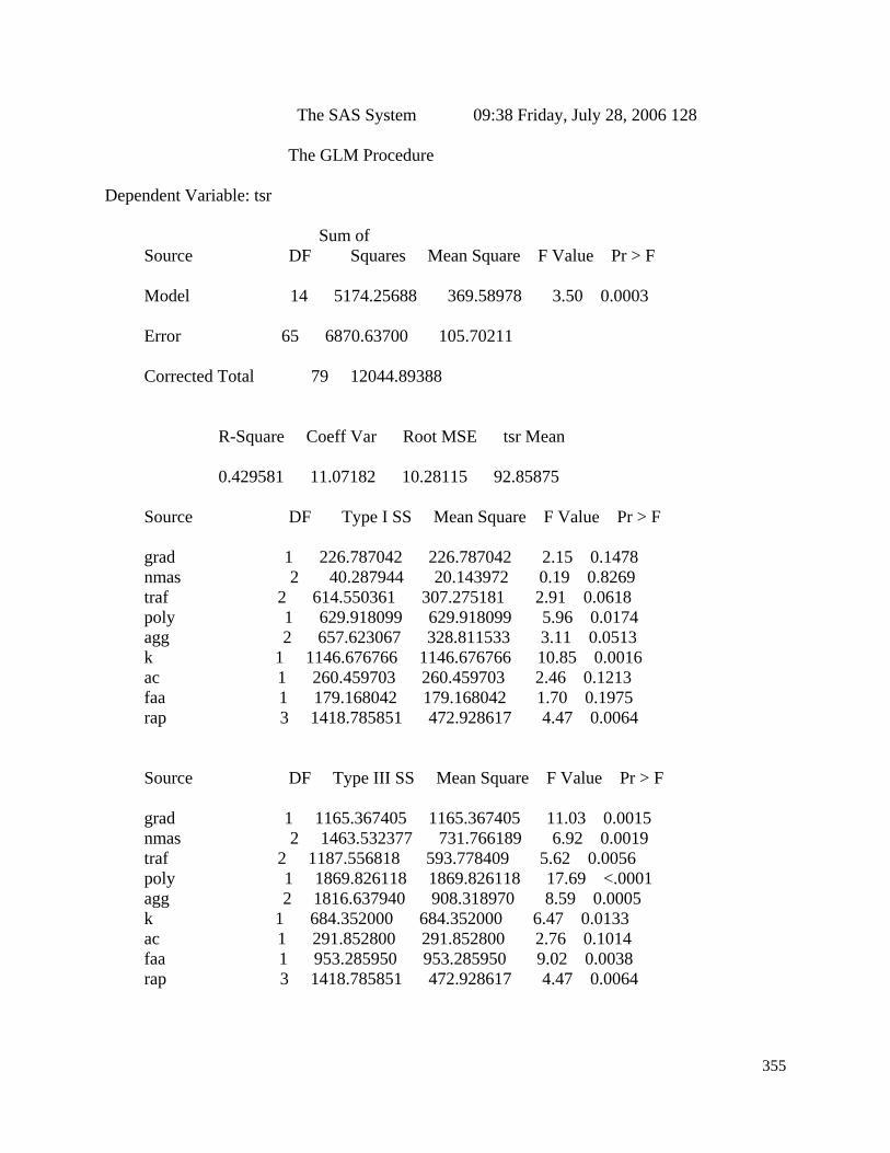
Table 8.42 Ratio of G*/sin(δ) of Specimens Tested in a Water Bath to Those Tested in an Air Chamber.......................................................................................................................... 210 Table 8.43 Ratio of G*/sin(δ) for Conditioned Water Bath Specimens Versus Unconditioned Air Chamber Specimens with Silica ..................................................................................... 211 Table 8.44 Factors with Levels Considered for Statistical Analysis .............................. 219 Table 8.45 GLM p-values Showing Statistically Significant Variables for TSR........... 221 Table 8.46 LSD Results for AASHTO T283.................................................................. 222 Table 8.47 GLM p-values Showing Statistically Significant Variables for E* Ratio .... 223 Table 8.48 LSD Results for E* Ratio ............................................................................. 223 Table 9.1 Summary of Moisture Damage Prone Materials ............................................ 229
xi
LIST OF FIGURES
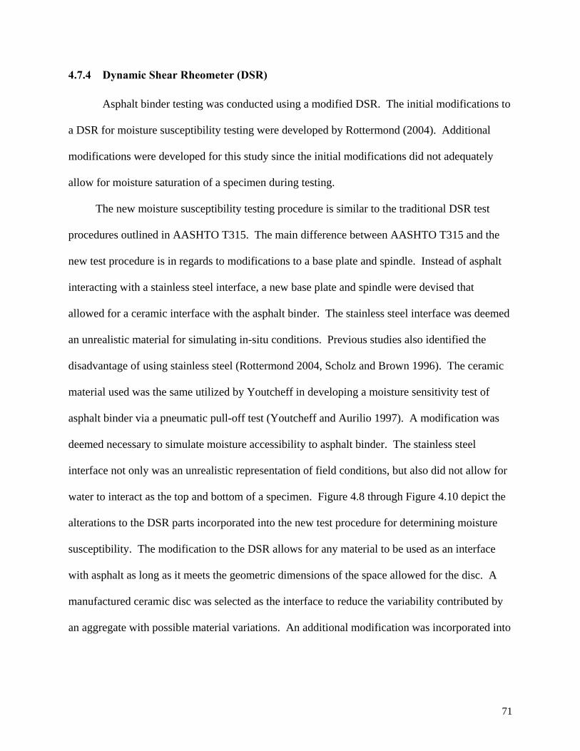
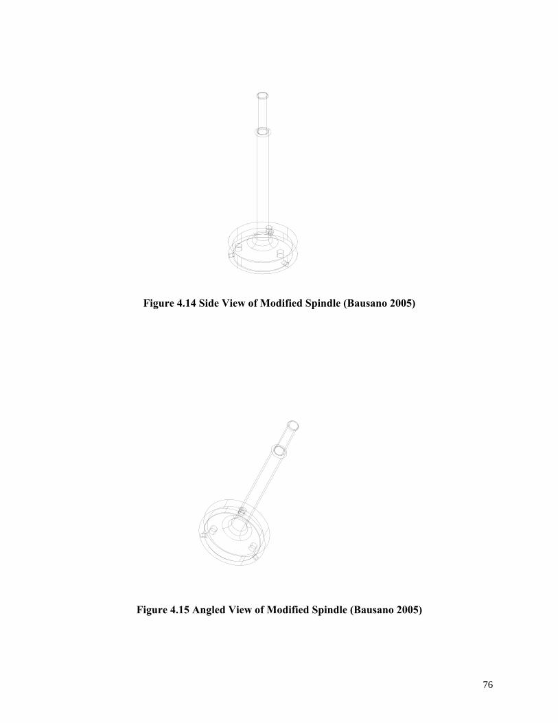
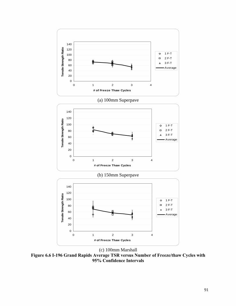
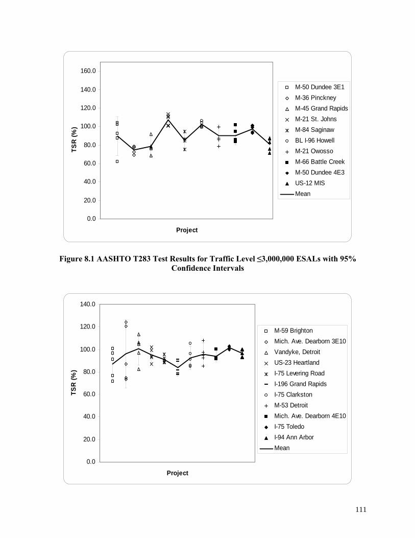
Figure 2.1 Haversine Loading Pattern or Stress Pulse for the Dynamic Modulus Test (Witczak et al. 2002)\ ........................................................................................................................... 37 Figure 2.2 Flow Number Loading (Robinette 2005) ........................................................ 39 Figure 3.1 Project Locations ............................................................................................. 46 Figure 3.2 Stockpile Cone Proportions (Robinette 2005)................................................. 47 Figure 4.1 ISU and Contractor JMF Gmm ......................................................................... 51 Figure 4.2 ISU and Contractor JMF Gmm ......................................................................... 52 Figure 4.3 ISU and Contractor Binder Contents............................................................... 55 Figure 4.4 ISU versus Contractor Binder Contents .......................................................... 56 Figure 4.5 Comparison of #200 Sieve .............................................................................. 57 Figure 4.6 Changes in Weight of Specimen After Gmb Determination ............................ 60 Figure 4.7 Air Voids Before and After Sawing/Coring.................................................... 63 Figure 4.8 Modified DSR Base plate................................................................................ 72 Figure 4.9 Modified DSR Spindle .................................................................................... 72 Figure 4.10 Modified DSR Spindle with Three Holes ..................................................... 73 Figure 4.11 Dimensions Of Modified Spindle( Bausano, 2005) ...................................... 74 Figure 4.12 View of Spindle Through The Base (Bausano 2005).................................... 75 Figure 4.13 View of Modified Spindle From Top Down (Bausano 2005)....................... 75 Figure 4.14 Side View of Modified Spindle (Bausano 2005) .......................................... 76 Figure 4.15 Angled View of Modified Spindle (Bausano 2005)...................................... 76 Figure 6.1 M-50 Dundee Average TSR versus Number of Freeze/thaw Cycles with 95% Confidence Intervals ......................................................................................................... 86 Figure 6.2 M-21 St. Johns Average TSR versus Number of Freeze/thaw Cycles with 95% Confidence Intervals ......................................................................................................... 87 Figure 6.3 BL I-96 Howell Average TSR versus Number of Freeze/thaw Cycles with 95% Confidence Intervals ......................................................................................................... 88 Figure 6.4 M-21 Owosso Average TSR versus Number of Freeze/thaw Cycles with 95% Confidence Intervals ......................................................................................................... 89 Figure 6.5 M-59 Brighton Average TSR versus Number of Freeze/thaw Cycles with 95% Confidence Intervals ......................................................................................................... 90 Figure 6.6 I-196 Grand Rapids Average TSR versus Number of Freeze/thaw Cycles with 95% Confidence Intervals ......................................................................................................... 91 Figure 6.7 I-75 Clarkston Average TSR versus Number of Freeze/thaw Cycles wit 95% Confidence Intervals ......................................................................................................... 92 Figure 6.8 Average TSR Results for Traffic Level ≤3,000,000 ESAL's .......................... 93 Figure 6.9 Average TSR Results for Traffic Level >3,000,000 ESAL's .......................... 93 Figure 6.10 100mm Marshall versus 150mm Superpave at one freeze/thaw cycle.......... 98 Figure 6.11 100mm Marshall versus 100mm Superpave at one freeze/thaw cycle.......... 99 Figure 6.12 100mm Marshall versus 150mm Superpave at one freeze/thaw cycle.......... 99 Figure 8.1 AASHTO T283 Test Results for Traffic Level ≤3,000,000 ESALs with 95% Confidence Intervals ....................................................................................................... 111 Figure 8.2 AASHTO T283 Test Results for Traffic Level >3,000,000 ESALs with 95% Confidence Intervals ....................................................................................................... 112 Figure 8.3 Dry Strength versus Wet Strength (Pooled Data).......................................... 112
xii
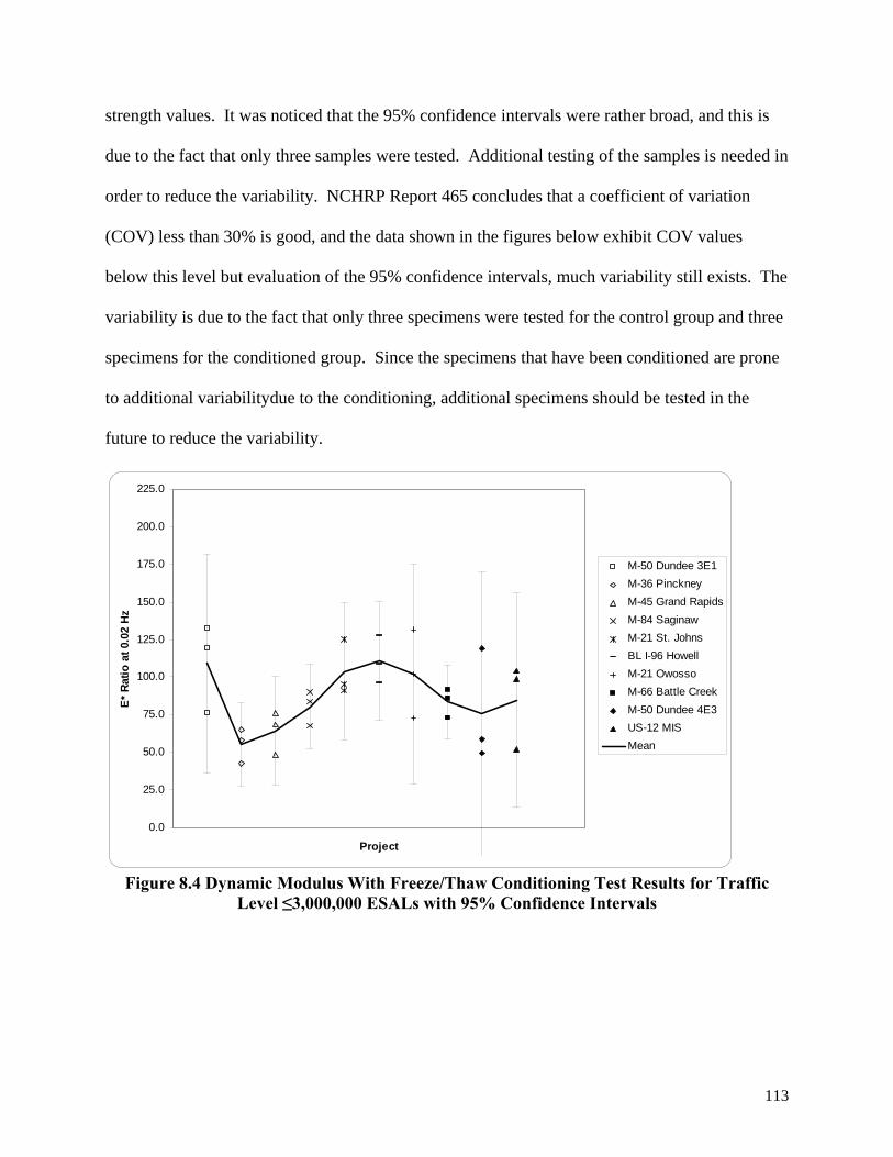
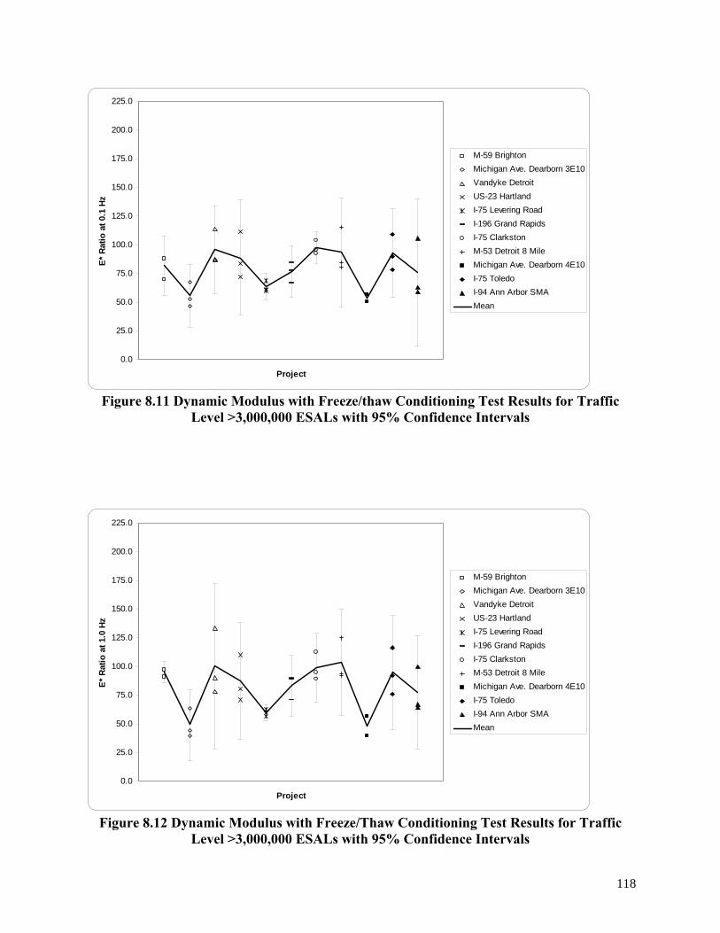
Figure 8.4 Dynamic Modulus With Freeze/Thaw Conditioning Test Results for Traffic Level ≤3,000,000 ESALs with 95% Confidence Intervals....................................................... 113 Figure 8.5 Dynamic Modulus with Freeze/Thaw Conditioning Test Results for Traffic Level ≤3,000,000 ESALs with 95% Confidence Intervals....................................................... 114 Figure 8.6 Dynamic Modulus with Freeze/Thaw Conditioning Test Results for Traffic Level ≤3,000,000 ESALs with 95% Confidence Intervals....................................................... 114 Figure 8.7 Dynamic Modulus with Freeze/Thaw Conditioning Test Results for Traffic Level ≤3,000,000 ESALs with 95% Confidence Intervals....................................................... 115 Figure 8.8 Dynamic Modulus with Freeze/Thaw Conditioning Test Results for Traffic Level ≤3,000,000 ESALs with 95% Confidence Intervals....................................................... 116 Figure 8.9 Dynamic Modulus with Freeze/Thaw Conditioning Test Results for Traffic Level ≤3,000,000 ESALs with 95% Confidence Intervals....................................................... 116 Figure 8.10 Dynamic Modulus With Freeze/Thaw Conditioning Test Results for Traffic Level >3,000,000 ESALs with 95% Confidence Intervals....................................................... 117 Figure 8.11 Dynamic Modulus with Freeze/thaw Conditioning Test Results for Traffic Level >3,000,000 ESALs with 95% Confidence Intervals....................................................... 118 Figure 8.12 Dynamic Modulus with Freeze/Thaw Conditioning Test Results for Traffic Level >3,000,000 ESALs with 95% Confidence Intervals....................................................... 118 Figure 8.13 Dynamic Modulus with Freeze/Thaw Conditioning Test Results for Traffic Level >3,000,000 ESALs with 95% Confidence Intervals....................................................... 119 Figure 8.14 Dynamic Modulus with Freeze/Thaw Conditioning Test Results for Traffic Level >3,000,000 ESALs with 95% Confidence Intervals....................................................... 120 Figure 8.15 Dynamic Modulus with Freeze/Thaw Conditioning Test Results for Traffic Level >3,000,000 ESALs with 95% Confidence Intervals....................................................... 120 Figure 8.16 Dry E* versus Wet E* (Pooled Data).......................................................... 121 Figure 8.17 Graphical Comparison of Environmental Testing Conditions for All Data 126 Figure 8.18 Complex Shear Modulus ............................................................................. 130 Figure 8.19 Comparison of Elastic and Viscous Percent Changes for Original Binders 131 Figure 8.20 Ann Arbor Confidence Ellipsoid................................................................. 133 Figure 8.21 Plot of Normalized Elastic and Viscous Differences .................................. 133 Figure 8.22 Confidence Ellipsoid for Battle Creek Original Binder .............................. 134 Figure 8.23 Plot of Normalized Viscous and Elastic Differences for Battle Creek ....... 135 Figure 8.24 Confidence Ellipsoid of Normalized Elastic and Viscous Differences of Brighton Original Binder ............................................................................................................... 136 Figure 8.25 Plot of Viscous and Elastic Component Normalized Differences for Brighton136 Figure 8.26 Confidence Ellipsoid for Elastic and Viscous Component Differences of Clarkston Original Binder ............................................................................................................... 137 Figure 8.27 Plot of Normalized Elastic and Viscous Component Differences for Clarkston......................................................................................................................................... 138 Figure 8.28 Confidence Ellipsoid of Normalized Elastic and Viscous Differences of Original Binder from Detroit......................................................................................................... 139 Figure 8.29 Plot of Normalized Elastic and Viscous Component Differences for Detroit Binder......................................................................................................................................... 139 Figure 8.30 Confidence Ellipsoid for Original Binder Dundee 19.0mm NMAS ........... 140 Figure 8.31 Plot of Normalized Elastic and Viscous Component Differences for Dundee 19.0mm NMAS Binder ................................................................................................................. 140
xiii
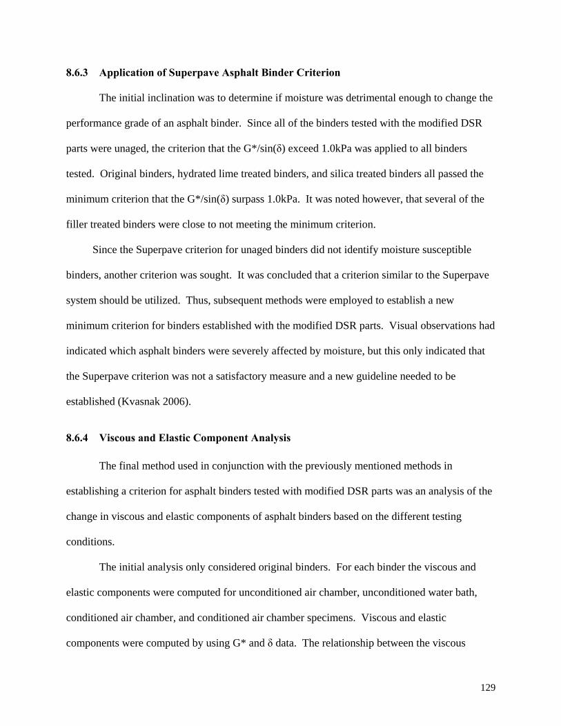
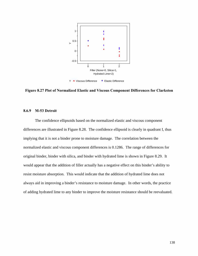
Figure 8.32 Confidence Ellipsoid of Dundee 12.5mm NMAS Original Binder ............ 141 Figure 8.33 Plot of Normalized Elastic and Viscous Component Differences for Dundee 12.5mm NMAS Binder ................................................................................................................. 142 Figure 8.34 Confidence Ellipsoid of Grand Rapids I-196 Original Binder.................... 143 Figure 8.35 Plot of Normalized Elastic and Viscous Component Differences for Grand Rapids I-196 Binder....................................................................................................................... 143 Figure 8.36 Confidence Ellipsoid for Grand Rapids M-45 Original Binder .................. 144 Figure 8.37 Plot of Normalized Elastic and Viscous Component Differences for Grand Rapids M-45 Original Binder ..................................................................................................... 144 Figure 8.38 Confidence Ellipsoid for Hartland Original Binder .................................... 145 Figure 8.39 Plot of Normalized Elastic and Viscous Component Differences for Hartland Binder......................................................................................................................................... 146 Figure 8.40 Confidence Ellipsoid for Howell Original Binder....................................... 147 Figure 8.41 Plot of Normalized Elastic and Viscous Component Differences for Howell Binder......................................................................................................................................... 147 Figure 8.42 Confidence Ellipsoid for Levering Original Binder.................................... 148 Figure 8.43 Plot of Normalized Elastic and Viscous Component Differences for Levering Binder......................................................................................................................................... 148 Figure 8.44 Confidence Ellipsoid for Michigan Ave 19.0mm NMAS Original Binder. 149 Figure 8.45 Plot of Normalized Elastic and Viscous Component Differences for Michigan Ave 19.0mm NMAS Binder................................................................................................... 149 Figure 8.46 Confidence Ellipsoid for Michigan Avenue 12.5mm NMAS Original Binder150 Figure 8.47 Overlay Plot of Normalized Elastic and Viscous Component Differences for Michigan Avenue 12.5mm NMAS Binder ..................................................................... 151 Figure 8.48 Confidence Ellipsoid for Michigan International Speedway US-12 Original Binder......................................................................................................................................... 152 Figure 8.49 Overlay Plot of Normalized Elastic and Viscous Component Differences for Michigan International Speedway US-12 Binder ........................................................... 152 Figure 8.50 Confidence Ellipsoid for Owosso Original Binder ..................................... 153 Figure 8.51 Overlay Plot of Normalized Elastic and Viscous Component Differences for Owosso Binder.............................................................................................................................. 153 Figure 8.52 Confidence Ellipsoid for Pinckney Original Binder ................................... 154 Figure 8.53 Overlay Plot of Normalized Elastic and Viscous Component Differences for Pinckney Binder.............................................................................................................. 155 Figure 8.54 Confidence Ellipsoid for Saginaw Original Binder..................................... 156 Figure 8.55 Overlay Plot of Normalized Elastic and Viscous Component Differences for Saginaw Binder............................................................................................................... 156 Figure 8.56 Confidence Ellipsoid of St. Johns Original Binder ..................................... 157 Figure 8.57 Overlay Plot of Normalized Elastic and Viscous Component Differences for St. Johns Binder.................................................................................................................... 157 Figure 8.58 Confidence Ellipsoid for Toledo Original Binder ....................................... 158 Figure 8.59 Overlay Plot of Normalized Elastic and Viscous Component Differences for Toledo Binder.............................................................................................................................. 158 Figure 8.60 Confidence Ellipsoid of Van Dyke Original Binder ................................... 159 Figure 8.61 Overlay Plot of Normalized Elastic and Viscous Component Differences for Van Dyke Binder .................................................................................................................... 159
xiv
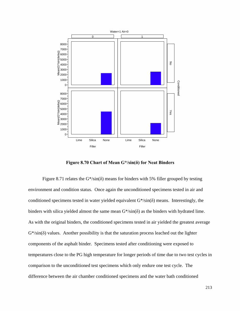
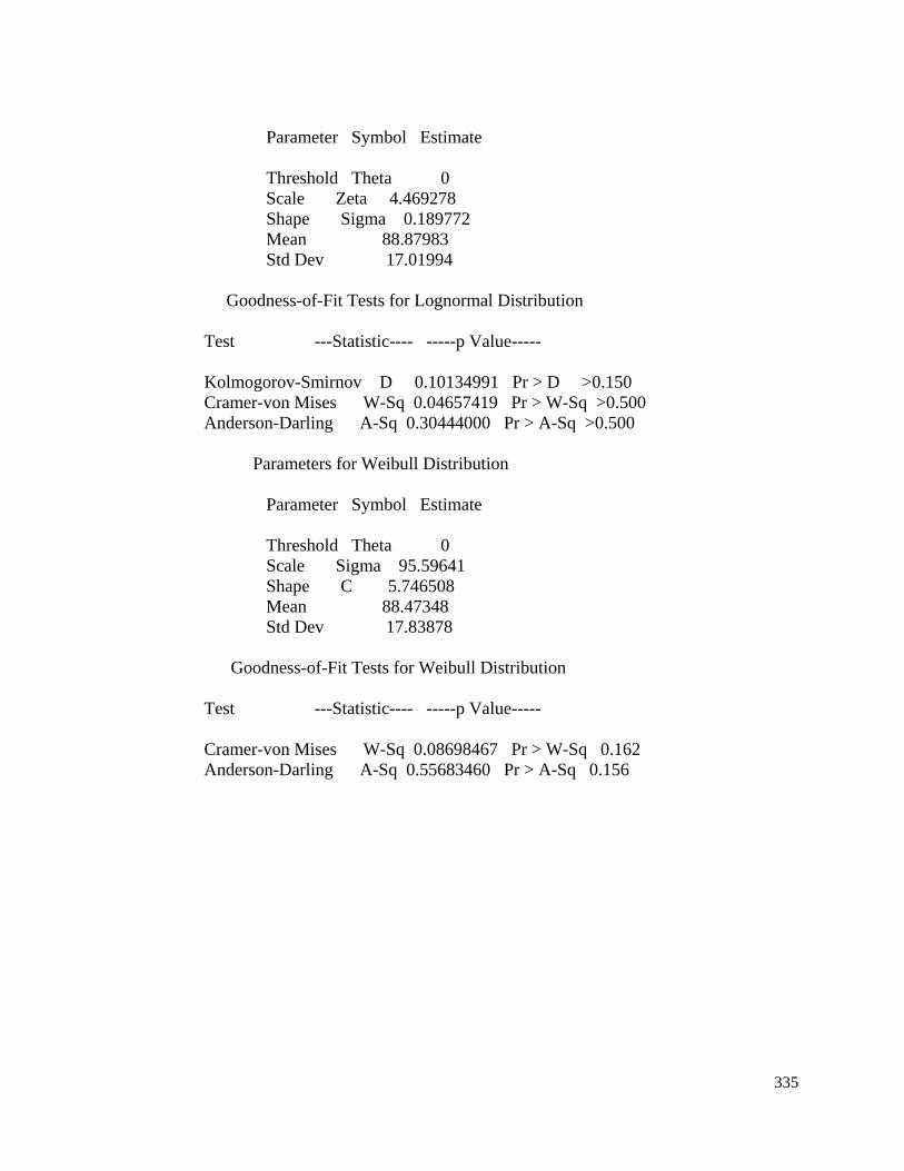
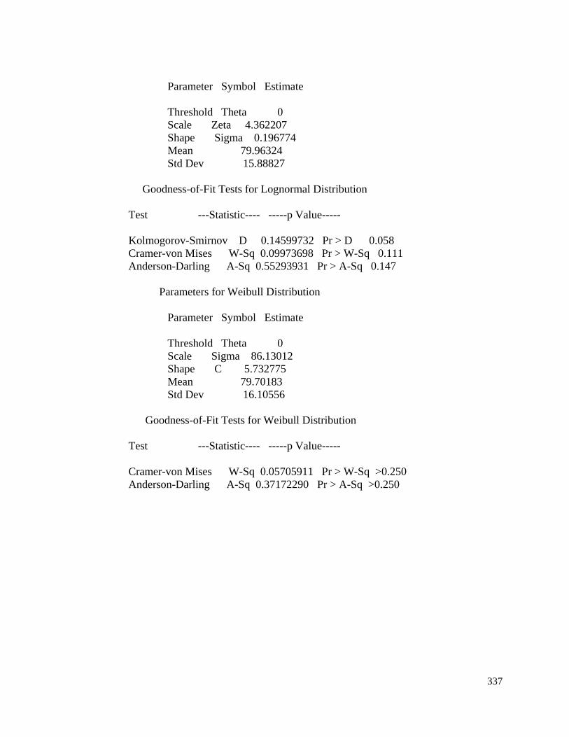
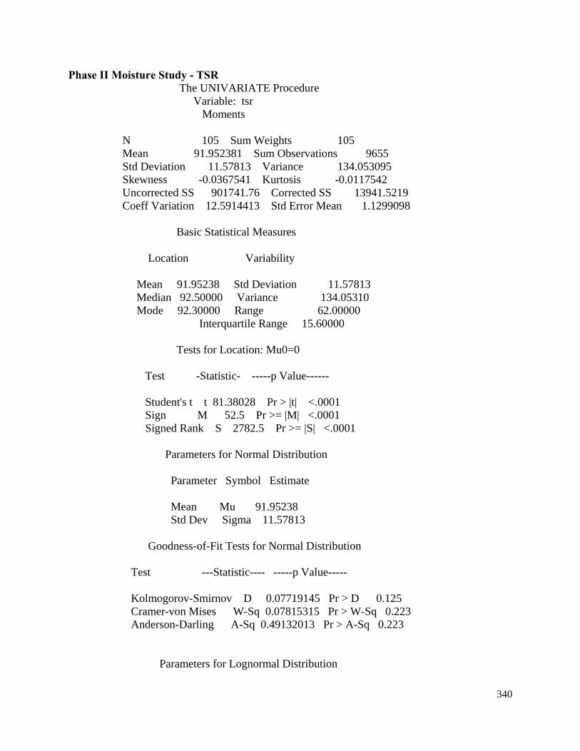
Figure 8.62 Lognormal Distribution of TSRs................................................................. 165 Figure 8.63 Lognormal Distribution of E* Ratios at 0.02 Hz ........................................ 167 Figure 8.64 Lognormal Distribution of E* Ratios at 0.1 Hz .......................................... 167 Figure 8.65 Lognormal Distribution of E* Ratios at 1.0 Hz .......................................... 168 Figure 8.66 Lognormal Distribution of E* Ratios at 5.0 Hz .......................................... 168 Figure 8.67 Lognormal Distribution of E* Ratios at 10.0 Hz ........................................ 169 Figure 8.68 Lognormal Distribution of E* Ratios at 25.0 Hz ........................................ 169 Figure 8.69 Variability Plot of G*/sin(δ)........................................................................ 212 Figure 8.70 Chart of Mean G*/sin(δ) for Neat Binders.................................................. 213 Figure 8.71 Chart of Mean G*/sin(δ) of Binders with 5% Filler.................................... 214 Figure 8.72 Chart of Mean G*/sin(δ) of Binders with 10% Filler.................................. 215 Figure 8.73 Chart of Mean G*/sin(δ) of Binders with 20% Filler.................................. 216 Figure 8.74 TSR versus Permeability ............................................................................. 220 Figure 8.75 TSR versus RAP.......................................................................................... 220 Figure 8.76 TSR versus Asphalt Content ....................................................................... 221
xv
LIST OF ACRONYMS
A Witczak Predictive Equation Regression Intercept APA Asphalt Pavement Analzyer AAPT Association of Asphalt Paving Technologists AASHTO American Association of State and Highway Transportation Officials ASTM American Society for Testing and Materials BSG (Gmb) Bulk Specific Gravity COV Coefficient of Variation CTAA Canadian Technical Asphalt Association D60 Grain size that corresponds to 60 percent passing DSR Dynamic Shear Rheometer E* and *E Complex Modulus and Dynamic Modulus, respectively
E’ and E” Elastic and Viscous Modulus, respectively ESAL Equivalent Single Axle Load FHWA Federal Highway Administration FN Flow Number Gb Asphalt Specific Gravity Gsb Aggregate Bulk Specific Gravity Gse Aggregate Effective Specific Gravity HRB Highway Research Board HMA Hot Mix Asphalt IDT Indirect Tension Test JMF Job Mix Formula LVDT Linear Variable Differential Transducer M-E Mechanistic-Empirical MTSG (Gmm) Maximum Theoretical Specific Gravity MTU Michigan Technological University NCAT National Center for Asphalt Technology NCHRP National Cooperative Highway Research Program NMAS Nominal Maximum Aggregate Size Pb Asphalt Binder Content Peff Effective Asphalt Binder Content R2 Coefficient of Determination RAP Recycled Asphalt Pavement RTFO Rolling Thin Film Oven SGC Superpave Gyratory Compactor SHRP Strategic Highway Research Program SSD Saturate Surface Dry SPT Simple Performance Test SST Superpave Shear Tester TAI The Asphalt Institute UTM Universal Testing Machine V Witczak Predictive Equation Regression Slope
xvi
VFA Voids Filled with Asphalt VMA Voids in the Mineral Aggregate εo Strain φ Phase Angle σo Stress
1
Executive Summary
Introduction
The accelerated damage of hot mix asphalt (HMA) due to moisture is of significant
concern to transportation agencies and researchers. It is of primary interest in the northern states
due to freeze/thaw action during the spring months, but it can be a problem wherever there is the
availability of moisture. Currently, there are many tests available to test HMA or binder to
determine if it is a mix, a binder, or both are moisture susceptible. Many of these tests have
produced varied results and a more mechanistic test is being sought that considers the micro-
mechanical behavior and/or chemical behavior of moisture damage. A significant amount of
time and money has been spent on trying to validate these tests and to determine how well the
results relate to the field performance of HMA.
Moisture susceptibility is the loss of strength in HMA mixtures due to the effects of
moisture. In HMA, there are three components: aggregates, asphalt binder, and air voids.
Moisture damage can occur in two ways; loss of adhesion between asphalt binder and aggregate,
or the weakening of asphalt mastic in the presence of moisture. Thus, selection of appropriate
aggregates (aggregate chemistry) and asphalt binder (binder chemistry) play an important role in
deterring moisture damage. Moisture damage can occur from a loss of adhesion between
aggregates and binder. This is due to the chemistry of the aggregates. Siliceous aggregate
sources are prone to stripping due to a high silica dioxide component. The asphalt binder cannot
bond to siliceous aggregate thus when moisture is present and HMA is loaded repeatedly, asphalt
binder strips from the aggregate resulting in a loss of adhesion (the binder holds the aggregates
together). Moisture damage is a significant concern because it diminishes the performance and
service life of HMA pavements resulting in increased maintenance and rehabilitation costs to
2
highway agencies. Moisture susceptibility is best identified by developing tests that illustrate the
effects of moisture damage whether it is on the HMA mixture or asphalt binder. Identification of
moisture susceptibility allows the issue to appropriately addressed if necessary.
Literature Review
According to Little and Jones (2003), moisture damage can be defined as the loss of
strength and durability in asphalt mixtures due to the effects of moisture. Moisture can damage
the HMA in two ways: 1) loss of bond between asphalt cement or mastic and fine and coarse
aggregates or 2) weakening of mastic due to the presence of moisture. There are six contributing
factors that have been attributed to causing moisture damage in HMA: detachment,
displacement, spontaneous emulsification, pore-pressure induced damage, hydraulic scour, and
environmental effects (Roberts et al. 1996, Little and Jones 2003). Not one of the above factors
necessarily works alone in damaging an HMA pavement, as several of these factors can have a
combined affect on damaging a pavement. Therefore there is a need to look at the adhesive
interface between aggregate and asphalt and the cohesive strength and durability of the mastic
(Graff 1986, Roberts et al. 1996, Little and Jones 2003, Cheng et al. 2003). A loss of the
adhesive bond between aggregate and asphalt can lead to stripping and raveling while a loss of
cohesion can lead to a weakened pavement that is susceptible to premature cracking and pore
pressure damage (Majidzadeh and Brovold 1966, Kandhal 1994, Birgission et al. 2003).
Several tests are available that are conducted on loose HMA mixtures, asphalt binders, or
compacted HMA mixtures. The most notable loose mixture test is the boiling water test. Some
notable asphalt binder tests are the pull-off tensile strength test and the Wilhelmy plate test.
Some widely used compacted mixture tests are AASHTO T283 (Lottman 1998, Lottman 1992,
Tunnicliff and Root 1982, Kennedy et al. 1983, Tunnicliff and Root 1984, Coplantz and
3
Newcomb 1988, Kennedy and Ping 1991, Stroup-Gardiner and Epps 1992, Epps et al. 2000),
Hamburg Wheel Track test device (Aschenbrener et al. 1995), Asphalt Pavement Analyzer
(APA) (Cross et al 2000, APA Manual 2002, Mallick et al. 2003, West et al. 2004, Johnston et al
2005), and the Environmental Conditioning System (ECS (Terrel et al. 1994). The current
method for evaluating the moisture susceptibility of compacted bituminous mixtures is
AASHTO T283. AASHTO T283 is based on the Marshall mix design method, but current
research and highway agencies are evaluating the moisture susceptibility of Superpave mixtures
based on AASHTO T283. The Superpave volumetric mix design procedure does not include a
simple, mechanical test that is analogous to the Marshall stability and flow test criteria. The
Superpave mix design system relies on material specifications and volumetric criteria in order to
ensure a quality performing mix design. Inclusion of AASHTO T283 in Superpave did not
consider the change in specimen size from 100mm to 150mm and resulted in the initiation of
NCHRP 9-13 in 1996 (Epps et al. 2000). The researchers concluded that either AASHTO T283
does not evaluate moisture susceptibility or the criterion, the tensile strength ratio (TSR), is
incorrectly specified. NCHRP 9-13 examined mixtures that have historically been moisture
susceptible and ones that have not. The researchers also examined the current criteria using
Marshall and Hveem compaction, which was considered in the previously mentioned
conclusions.
The procedures in AASHTO T283 and NCHRP 9-13 consider the loss of strength due to
freeze/thaw cycling and the effects of moisture existing in specimens compared to unconditioned
specimens. However, mixtures do not experience such a pure phenomenon. Pavements undergo
cycling of environmental conditions, but when moisture is present, there is repeated hydraulic
loading with development of pore pressure in mixtures. Thus, AASHTO T283 and the NCHRP
4
9-13 study do not consider the effect of pore pressure, but rather consider a single load effect on
environmentally conditioned specimens. This project has developed moisture susceptibility
procedures which utilizes the dynamic loading of specimens in saturated conditions and
compared to the results to unconditioned specimens in a dry test environment. The developed
test procedure considered the simple performance test, AASHTO T283, and the APA to
determine the moisture susceptibility of the mixtures.
Material Collection
During the summer of 2004, when the majority of sampling occurred, it was realized that
not all of the mixes could be sampled during the 2004 construction season. Thus, it was decided
that previous HMA mixtures that were sampled during the 2000 construction season could be
used coupled with additional sampling during the 2005 construction season. The 2000
construction projects that were sampled were stored in a heated, metal building where the
material was protected from rain, heat, and snow.
This research was been divided into two phases. Phase I testing was used to determine
the number of freeze/thaw cycles that will cause the equivalent damage to AASHTO T283
specimens for different methods of compaction and specimen sizes. Phase II testing of mixes for
moisture damage used the results of Phase I for AASHTO T283 testing on 150mm specimens
and the results of Phase I and Phase II for dynamic modulus testing. APA testing was based on
results from Phase I. In the ensuing sections, the mixture experimental plan and laboratory
testing experimental plan are outlined.
The experimental plan considers different mix types, aggregate sources, laboratory test
systems, conditioning approaches, and test specimen size. The experimental plan includes two
integrated plans: one for the mixes and one for the planned laboratory tests. A sensitivity study
5
on the effects of specimen size and compaction method was conducted on a limited number of
mixes to determine the amount of conditioning that should be needed on larger Superpave
compacted specimens to obtain analogous conditioning as AASHTO T283 Marshall mix
specimens. Table 1 below outlines the sensitivity study experimental plan.
Table 1 Sensitivity Study Experimental Plan for Mix and Aggregate Types
≤ 3,000,000 >3,000,000Limestone - M50 Dundee Limestone - M59 BrightonGravel - M21 St. JohnsLimestone - BL96 Howell Limestone - I-196 Grand RapidsGravel - M21 Owosso Slag/Trap Rock - I-75 Clarkston
PHASE 1 MOISTURETraffic Level (ESAL)
25.0 or 19.0
12.5 or 9.5
NMAS (mm)
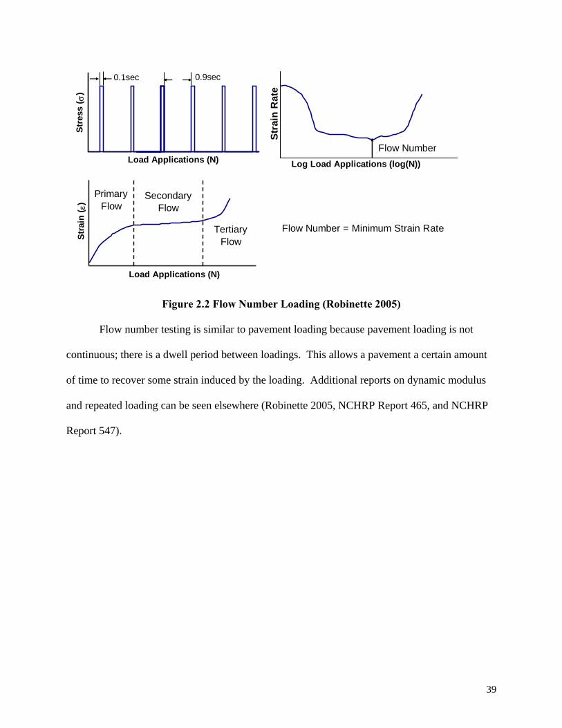
The Phase II experimental plan considers different mix types, aggregate sources, and
laboratory test systems. Table 2 below outlines the expanded experimental plan.
Table 2 Expanded Experimental Plan for Phase II Projects
The immersion-compression test (ASTM D1075 and AASHTO T165-155) is among the
first moisture sensitivity tests developed based on testing 100mm diameter compacted
specimens. A more detailed explanation of this test can be reviewed in ASTM Special Technical
Publication 252 (Goode 1959). This test consists of compacting two groups of specimens: a
control group and a moisture conditioned group at an elevated temperature (48.8°C water bath)
for four days (Roberts et al. 1996). The compressive strength of the conditioned and control
group are then measured (Roberts, et al. 1996). The average strength of the conditioned
specimens over that of the control specimens is a measure of strength lost due to moisture
28
damage (Solaimanian et al. 2003). Most agencies specify a minimum retained compressive
strength of 70%.
2.5.2.2 Marshall Immersion Test
The procedure for producing and conditioning two groups of specimens is identical to the
immersion-compression test. The only difference is, the Marshall stability test is used as the
strength parameter as opposed to the compression test (Solaimanian et al. 2003). A minimum
retained Mashall stability number could not be found in the literature.
2.5.2.3 Moisture Vapor Susceptibility
The moisture vapor susceptibility test was developed by the California Department of
Transportation (California Test Method 307). A California kneading compactor is used to
compact two specimens. The compacted surface of each specimen is sealed with an aluminum
cap and a silicone sealant is applied to prevent the loss of moisture (Solaimanian, et al. 2003).
After the specimens have been conditioned at an elevated temperature and suspended over water,
testing of the specimens commences. The Hveem stabilometer is used to test both dry and
moisture conditioned specimens. A minimum Hveem stabilometer value is required for moisture
conditioned specimens, which is less than that required for dry specimens used in the mix design
(Solaimanian et al. 2003).
2.5.2.4 Repeated Pore Water Pressure Stressing and Double-Punch Method
The repeated pore water pressure stressing and double punch method was developed by
Jimenez at the University of Arizona (1974). This test accounts for the effects of dynamic traffic
loading and mechanical properties. In order to capture the effects of pore water pressure, the
specimens are conditioned by a cyclic stress under water. After the specimen has undergone the
pore pressure stressing the tensile strength is measured using the double punch equipment.
29
Compacted specimens are tested through steel rods placed at either end of the specimen in a
punching configuration.
2.5.2.5 Original Lottman Method
The original Lottman test was developed at the University of Idaho by Robert Lottman
(1978). The laboratory procedure consists of compacting three sets of 100mm diameter by
63.5mm Marshall specimens to be tested dry or under accelerated moisture conditioning
(Lottman et al. 1974). Below are the following laboratory conditions for each of the groups:
• Group 1: Control group, dry;
• Group 2: Vacuum saturated with water for 30-minutes; and
• Group 3: Vacuum saturation followed by freeze cycle at -18°C for 15- hours and
then subjected to a thaw at 60°C for 24-hours (Lottman et al. 1974).
After the conditioning phase the indirect tensile equipment is used to conduct tensile
resilient modulus and tensile strength of conditioned and dry specimens. All specimens are
tested at 13°C or 23°C at a loading rate of 1.65mm/min. The severity of moisture damage is
based on a ratio of conditioned to dry specimens (TSR) (Lottman et al. 1974, Lottman 1982). A
minimum TSR value of 0.70 is recommended (NCHRP 246). Laboratory compacted specimens
were compared to field cores and plotted against each other on a graph. The laboratory and field
core specimens line up fairly close to the line of equality.
2.5.2.6 Modified Lottman Test (AASHTO T283)
“Resistance of Compacted Bituminous Mixture to Moisture Induced Damage” AASHTO
T283, is the most commonly used test method for determining moisture susceptibility of HMA.
This test is similar to the original Lottman test with only a few exceptions which are:
• Two groups, control versus moisture conditioned,
30
• Vacuum saturation until a saturation level of 70% to 80% is achieved, and
• Test temperature and loading rate change to 50mm/min at 25ºC.
A minimum TSR value of 0.70 is recommended (Roberts et al., 1996). AASHTO T283
was adopted by the Superpave system as the moisture test method of choice even though
AASHTO T283 was developed for Marshall mixture design. State highway agencies have
reported mixed results when using AASHTO T283 and comparing the results to field
performance (Stroup-Gardiner et al. 1992, Solaimanian et al. 2003). NCHRP Project 9-13
looked at different factors affecting test results such as types of compaction, diameter of
specimen, degree of saturation, and freeze/thaw cycles. Conclusions from looking at the
previously mentioned factors can be seen in the NCHRP 9-13 report (Epps et al. 2000). The
researchers concluded that either AASHTO T283 does not evaluate moisture susceptibility or the
criterion, TSR, is incorrectly specified. NCHRP 9-13 examined mixtures that have historically
been moisture susceptible and ones that have not. The researchers also examined the current
criteria using Marshall and Hveem compaction. A recent study at the University of Wisconsin
found no relationship exists between TSR and field performance in terms of pavement distress
index and moisture damage (surface raveling and rutting) (Kanitpong et al. 2006). Additional
factors such as production and construction, asphalt binder and gradation play important roles.
Mineralogy does not appear to be an important factor in relation to pavement performance.
2.5.2.7 ASTM D4867 (Tunnicliff-Root Test Procedure)
“Standard Test Method for Effect of Moisture on Asphalt Concrete Paving Mixtures,”
ASTM D4867 is comparable to AASHTO T283. The only difference between AASHTO T283
and ASTM D4867 is that the curing of loose mixture at 60°C in an oven for 16 hours is
31
eliminated in ASTM D4867. A minimum TSR of 0.70 to 0.80 are specified by highway
agencies (Roberts et al. 1996).
2.5.2.8 Texas Freeze/Thaw Pedestal Test
The water susceptibility test was developed by Plancher et al. (1980) at Western Research
Institute but was later modified into the Texas freeze/thaw pedestal by Kennedy et al. (1983).
Even though this test is rather empirical in nature, it is fundamentally designed to maximize the
effects of bond and to minimize the effects of mechanical properties such as gradation, density,
and aggregate interlock by using a uniform gradation (Kennedy et al. 1983). An HMA briquette
is made according to the procedure outlined by Kennedy et al. (1982). The specimen is then
placed on a pedestal in a jar of distilled water and covered. The specimen is subjected to thermal
cycling and inspected each day for cracks. The number of cycles to induce cracking is a measure
of the water susceptibility (Kennedy et al. 1983). The benefits of running this test are some key
failures can be seen:
• Bond failure at the asphalt-aggregate interface (stripping) and
• Fracture of the thin asphalt films bonding aggregate particles (cohesive failure) by
formation of ice crystals (Solaimanian et al. 2003).
2.5.2.9 Hamburg Wheel-Tracking Device (HWTD)
The Hamburg wheel tracking device was developed by Esso A.G. and is manufactured by
Helmut-Wind, Inc. of Hamburg, Germany (Aschenbrener et al. 1995, Romero and Stuart 1998).
Two samples of hot mix asphalt beams with each beam having a geometry of 26mm wide,
320mm long, and 40mm thick. This device measures the effects of rutting and moisture damage
by running a steel wheel over the compacted beams immersed in hot water (typically 50ºC)
(Aschenbrener et al. 1995). The steel wheel is 47mm wide and applies a load of 705N while
32
traveling at a maximum velocity of 340mm/sec in the center of the sample. A sample of HMA is
loaded for 20,000 passes or 20mm of permanent deformation occurs (Aschenbrener et al. 1995).
Some important results the HWTD gives are:
• Postcompaction consolidation: Deformation measured after 1,000 wheel passes;
• Creep Slope: Number of wheel passes to create a 1 mm rut depth due to viscous
flow;
• Stripping Slope: Inverse of the rate of deformation in the linear region of the
deformation curve; and
• Stripping Inflection Point: Number of wheel passes at the intersection of the
creep slope and stripping slope (Aschenbrener et al. 1995).
2.5.2.10 Asphalt Pavement Analyzer
The APA is a type of loaded wheel test. Rutting, moisture susceptibility, and fatigue
cracking can all be examined with an APA. The predecessor to the APA is the Georgia Loaded
Wheel Tester (GLWT). Similar to the GLWT, an APA can test either cylindrical or rectangular
specimens. Using either specimen geometry, the conditioned and unconditioned samples are
subjected to a steel wheel that transverses a pneumatic tube, which lies on top of an asphalt
sample. As the wheel passes back and forth over the tube, a rut is created in a sample.
Numerous passes lead to a more defined rut and eventually, stress fractures can begin to manifest
as cracks. Modeling these ruts and cracks helps to predict how different combinations of
aggregate and binder for given criteria such as temperature and loading, will react under varying
circumstances. The conditioning of a sample is based upon the characteristic an APA is testing.
One of the main differences between an APA and a GLWT is an APA’s ability to test samples
33
under water as well as in air. Testing submerged samples allows researchers to examine
moisture susceptibility of mixes (Cooley et al. 2000).
An APA results are comparable to field data. A study that compared WesTrack, a full-
scale test track, data with APA results found a strong relationship between field data and
laboratory data (Williams and Prowell 1999). An additional study at the University of Tennessee
revealed that an APA sufficiently predicted the potential for rutting of 30 HMAs commonly used
in Tennessee (Jackson and Baldwin 1999).
To test moisture susceptible HMA samples, specimens are created in the same manner as
the specimens for testing rutting potential without moisture. The samples are placed in an APA,
which has an inner box that can be filled with water. The samples are completely submerged at
all times during testing; therefore effects of evaporation do not need to be taken into account.
The water bath is heated to a desired test temperature and the air in the chamber is also heated to
the same desired test temperature.
2.5.2.11 Environmental Conditioning System (ECS)
The ECS was developed by Oregon State University as part of the SHRP-A-403 and later
modified at Texas Technological University (Alam et al. 1998). The ECS subjects a membrane
encapsulated HMA specimen that is 102mm in diameter by 102mm in height to cycles of
temperature, repeated loading, and moisture conditioning (SHRP-A-403 1992, Al-Swailmi et al.
1992, Al-Swailmi et al. 1992, Terrel et al. 1993). Some important fundamental material
properties are obtained from using an ECS. These properties are resilient modulus (MR) before
and after conditioning, air permeability, and a visual estimation of stripping after a specimen has
been split open (SHRP-A-403, 1992). One of the significant advantages of using an ECS is the
ability to influence the HMA specimens to traffic loading and the resulting effect of pore water
34
pressure (Solaimanian et al. 2003) which is close to field conditions. The downfall of the test is,
it does not provide a better relationship to field observation than what was observed using
AASHTO T283. Also, AASHTO T283 is much less expensive to run and less complex than the
ECS.
2.5.2.12 Flexural Fatigue Beam Test with Moisture Conditioning
Moisture damage has been known to accelerate fatigue damage in pavements. Therefore,
conditioning of flexural fatigue beams was completed by Shatnawi et al. (1995). Laboratory
compacted beams were prepared from HMA sampled at jobs and corresponding field fatigue
beams were cut from the pavement. The conditioning of the beams is as follows:
• Partial vacuum saturation of 60% to 80%;
• Followed by 3 repeated 5-hour cycles at 60ºC followed by 4-hours at 25ºC while
remaining submerged; and
• One 5-hour cycle at -18ºC (Shatnawi et al. 1995).
The specimens are then removed from a conditioning chamber and tested according to AASHTO
TP8. Initial stiffness and fatigue performance were affected significantly by conditioning the
specimens (Shatnawi et al. 1995).
2.5.2.13 ECS/Simple Performance Test Procedures
As a result of NCHRP Projects 9-19, 9-29, and 1-37; new test procedures such as simple
performance tests (SPTs) are being evaluated. According to Witczak et al. (2002), an SPT is
defined as “A test method(s) that accurately and reliably measures a mixture response or
characteristic or parameter that is highly correlated to the occurrence of pavement distress (e.g.
cracking and rutting) over a diverse range of traffic and climatic conditions.” The mechanical
tests being looked at are the dynamic modulus |E*|, repeated axial load (FN), and static axial
35
creep tests (FT). These tests are conducted at elevated temperatures to determine a mixtures
resistance to permanent deformation. The dynamic modulus test is conducted at an intermediate
and lower test temperature to determine a mixtures susceptibility to fatigue cracking. Witczak et
al. (2002) have shown that dynamic modulus, flow time, and flow number yield promising
correlations to field performance. The advantages and disadvantages can be seen in Table 2.3
from the work of Brown et al. (2001) and Witczak et al. (2002).
36
Table 2.3 SPT Advantages and Disadvantages (Witczak et al. 2002 and Brown et al. 2001)
Test Parameter Test Condition Model R2 Se/Sy Advantages Disadvantages
Dynamic Modulus E*/sinφ
Sinusoidal Linear 130°F 5 Hz
Power 0.91 0.310
Direct input for 2002 Pavement Design Guide Not forced to use master curves Easily linked to established regression equations Non destructive tests
Coring and sawing Arrangement of LVDTs Confined testing gave poor results Need further study of reliability of confined open graded specimens Equipment is more complex Difficult to obtain 1.5:1height-to-diameter ratio specimens in lab
Repeated Loading (Flow Number)
FN
Unconfined 130°F Various Frequencies
Power 0.88 0.401 Better simulates traffic conditions
Equipment is more complex Restricted test temperature and load levels does not simulate field conditions Difficult to obtain 1.5:1height-to-diameter ratio specimens in lab
NCHRP 9-34 is currently looking at the aforementioned tests along with the ECS to
develop new test procedures to evaluate moisture damage (Solaimanian et al. 2003).
Solaimanian et al. (2006) reported that the results of the Phase I and Phase II testing of NCHRP
9-34 show that the dynamic complex modulus (DCM) test should be coupled with the ECS for
moisture sensitivity testing. Some preliminary findings out of NCHRP 9-34 show that the
ECS/DM test appear to separate good performing mixes from poor performing mixes in the field
compared with TSR testing from ASTM D4867. The dynamic complex modulus is determined
by applying a uniaxial sinusoidal vertical compressive load to an unconfined or confined HMA
cylindrical sample as shown in Figure 2.1.
37
Figure 2.1 Haversine Loading Pattern or Stress Pulse for the Dynamic Modulus Test (Witczak et al. 2002)\
The stress-to-strain relationship under a continuous sinusoidal load pattern for a liner
viscoelastic material is defined by the complex modulus (dynamic modulus), E*.
Mathematically, E* is equal to the maximum peak dynamic stress (σo) divided by the peak
recoverable strain (εo):
* o
o
E σε
= (equation 2.1)
The real and imaginary parts of the dynamic modulus can be written as
* ' ''E E iE= + (equation 2.2)
The previous equation shows that E* has two components; a real and an imaginary component.
E' is referred to as the storage or elastic modulus component, while E'' is referred to as the loss or
viscous modulus. The angle by which the peak recoverable strain lags behind the peak dynamic
stress is referred to as the phase angle, φ. The phase angle is an indicator of the viscous
properties of the material being evaluated.
Mathematically, this is expressed as
φφ sin|*|cos|*|* EiEE += (equation 2.3)
38
360×=p
i
tt
φ (equation 2.4)
where
ti = time lag between a cycle of stress and strain(s),
tp = time for a stress cycle(s), and
i = imaginary number.
For a purely viscous material, the phase angle is 90°, while for a purely elastic material
the phase angle is 0° (NCHRP 465 2002). The dynamic modulus, a measurable, “fundamental”
property of an HMA mixture is the relative stiffness of a mix. Mixes that have a high stiffness at
elevated temperatures are less likely to deform. But, stiffer mixes at an intermediate test
temperature are more likely to crack for thicker pavements (Shenoy and Romero 2002).
Therefore, the dynamic modulus test is conducted at intermediate and elevated temperatures to
evaluate the fatigue properties and the rutting propensity of HMA.
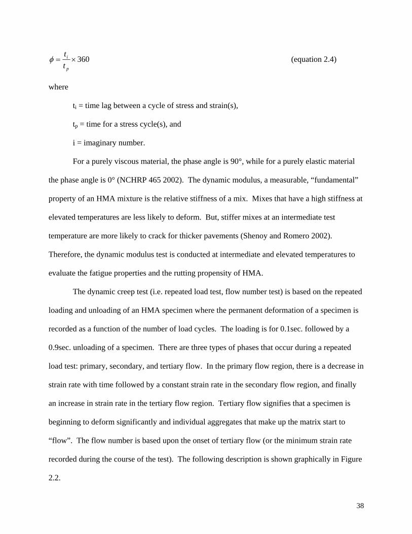
The dynamic creep test (i.e. repeated load test, flow number test) is based on the repeated
loading and unloading of an HMA specimen where the permanent deformation of a specimen is
recorded as a function of the number of load cycles. The loading is for 0.1sec. followed by a
0.9sec. unloading of a specimen. There are three types of phases that occur during a repeated
load test: primary, secondary, and tertiary flow. In the primary flow region, there is a decrease in
strain rate with time followed by a constant strain rate in the secondary flow region, and finally
an increase in strain rate in the tertiary flow region. Tertiary flow signifies that a specimen is
beginning to deform significantly and individual aggregates that make up the matrix start to
“flow”. The flow number is based upon the onset of tertiary flow (or the minimum strain rate
recorded during the course of the test). The following description is shown graphically in Figure
2.2.
39
Flow Number = Minimum Strain Rate
Load Applications (N)
Stre
ss ( σ
)0.1sec 0.9sec
Load Applications (N)
Stra
in ( ε
)
Primary Flow
Secondary Flow
TertiaryFlow
Log Load Applications (log(N))
Stra
in R
ate
Flow Number
Figure 2.2 Flow Number Loading (Robinette 2005)
Flow number testing is similar to pavement loading because pavement loading is not
continuous; there is a dwell period between loadings. This allows a pavement a certain amount
of time to recover some strain induced by the loading. Additional reports on dynamic modulus
and repeated loading can be seen elsewhere (Robinette 2005, NCHRP Report 465, and NCHRP
Report 547).
40
CHAPTER 3 EXPERIMENTAL PLAN
3.1 Experimental Plan
This research has been divided into two phases. Phase I testing was used to determine
the number of freeze/thaw cycles that will cause the equivalent damage to AASHTO T283
specimens. Phase II testing of mixes for moisture damage used the results of Phase I for the
AASHTO T283 testing on 150mm specimens and the results of Phase I and Phase II for dynamic
modulus testing. In the following sections below, the mixture experimental plan and laboratory
testing experimental plan is outlined.
3.1.1 Phase I Testing – Sensitivity Study
The experimental plan considers different mix types, aggregate sources, laboratory test
systems, and conditioning approaches. The experimental plan includes two integrated plans: one
for mixes and one for laboratory tests. A sensitivity study on the effects of specimen size and
compaction method was conducted on a limited number of mixes to determine the amount of
conditioning that should occur for larger Superpave compacted specimens. Table 3.1 below
outlines the sensitivity study experimental plan.
Table 3.1 Sensitivity Study Experimental Plan for Mix and Aggregate Types
Source of Variation SS df MS F P-value F critProject 5.61219 20 0.28061 4.93948 0.00038 2.12416Method 0.75201 1 0.75201 13.2374 0.00164 4.35124Error 1.13619 20 0.05681
Total 7.50039 41
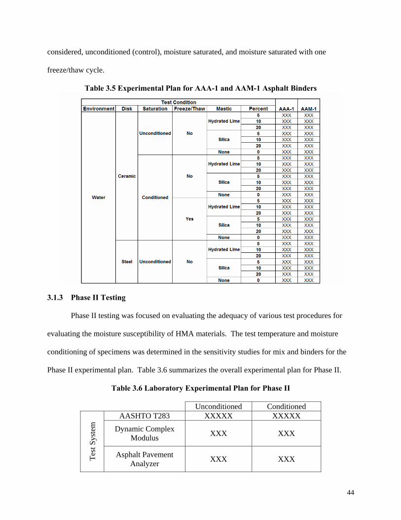
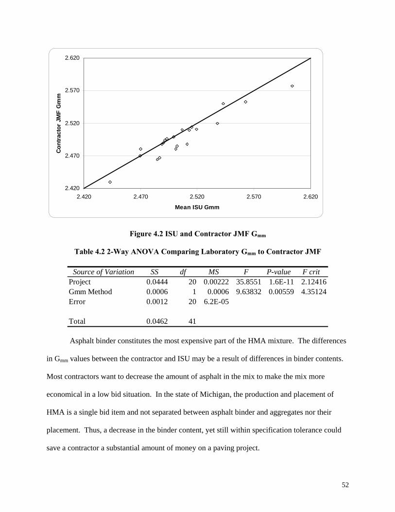
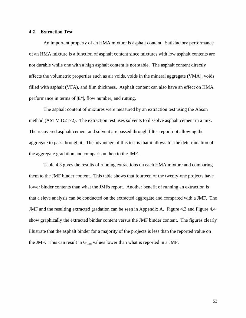
After solvents are used to dissolve the asphalt cement off of the aggregate, then the
asphalt cement and solvent are passed through filter report not allowing the aggregate to pass
through. The advantage of this test is that it allows for the determination of the aggregate
gradation and comparison then to the JMF. Two-way ANOVAs with no interaction were used at
each sieve size to determine if the percentage of the aggregate weight has changed on the sieves.
Table 4.5 shows that the gradation at each sieve size is statistically the same except at the #200
sieve where statistical differences result. For the most part the contractor’s JMF compares well
with the gradation from the extraction procedure. Figure 4.5 shows a comparison of the sieve
analysis results from the #200 sieve. The figure shows that there is a difference in #200 material
between the contractor JMF and the results from the extraction and sieve analysis.
Sieve Size (mm) 2-Way ANOVA ResultsJMF vs. Extraction
1 (25) Statistically the Same3/4 (19) Statistically the Same
1/2 (12.5) Statistically the Same3/8 (9.5) Statistically the Same#4 (4.75) Statistically the Same#8 (2.36) Statistically the Same#16 (1.18) Statistically the Same#30 (0.60) Statistically the Same#50 (0.30) Statistically the Same
#100 (0.15) Statistically the Same#200 (0.075) Statistically Different
0
1
2
3
4
5
6
7
8
9
0 1 2 3 4 5 6 7 8 9
#200 Sieve - Extraction
#200
Sie
ve -
JMF
#200 SieveSeries2
Figure 4.5 Comparison of #200 Sieve 4.2.1 Superpave Gyratory Compaction
Superpave gyratory specimens were compacted with a Pine AFGC125X SGC. The
100mm diameter specimens were compacted to approximately 63.5mm in height and the 150mm
diameter specimens were compacted to approximately 95mm in height for Phase I. For Phase II,
58
150mm diameter specimens were compacted to 95mm in height for AASHTO T283 testing and
APA testing. Dynamic complex modulus specimens were compacted to 170mm in height. All
specimens were compacted to 7±1% air voids. An assumed appropriate correction factor was
used based on gradation and NMAS. A new correction factor was calculated if the air voids
were out of range and additional specimens were procured.
4.2.2 Marshall Compaction
The Marshall compaction method was only used for Phase I of this research project. A
double-sided, automated Marshall hammer was used to compact specimens that were 100mm by
63.5mm in height. A double-sided mechanical compactor was selected instead of using the hand
compactor for three reasons; first, the variability of the compaction procedure would be
minimized, secondly, if this study was extended further, the compaction procedure would be
uniform, and thirdly, 140 specimens had to be procured so this method was better suited for mass
production of the samples. Before performance specimens could be procured, the determination
of the number of blows to achieve 7±1% air voids was needed for each mix. Four specimens per
job were compacted to 10, 25, 75 and 125 blows per side. A graph of air voids versus number of
blows per side was used to determine the number of blows required to achieve 7±1% air voids.
4.3 Compaction of Gyratory and Marshall Specimens
In Michigan, mix designs are based on compacting specimens to Ndes, which allows for
the air voids of the specimen to be measured according to AASHTO T166. In order to compact
gyratory specimens, a correction factor is needed to compact the specimens to height. The ratio
of the estimated Gmb via volumetric measurements of weight, height, and diameter to that of the
measured Gmb via saturated surface dried constitutes the correction factor. Typically, HMA
mixtures have a correction factor of 1.0 to 1.03. For Phase I and Phase II Superpave gyratory
59
specimens, a correction factor of 1.02 was used for fine mixes and a correction factor of 1.04 was
used for coarse mixtures. The correction factor was refined when the measured air voids were
not between 7±1% and additional specimens were procured with a new correction factor and the
air voids measured again. For the Marshall specimens, the sample mass was kept constant and
graphs of air voids versus number of blows were constructed for each project. The number of
blows to achieve 7% air voids was estimated from the graphical relationship for each mix. The
air voids were measured for the specimens and if they were not within 7±1% then additional
specimens were made by adjusting the number of blows.
All Superpave gyratory specimens for Phase I and Phase II were compacted with a Pine
Superpave Gyratory (SGC) model AFGC125X. This machine was selected because of its
familiarity and higher production capability. The SGC was fully calibrated to ensure that the
specimens were compacted to the correct height at an angle of 1.25° with a pressure of 600kPa in
accordance with Superpave compaction criterion.
Samples were split according to the weights required to achieve 63.5, 95, and 170mm for
the SGC specimens. The Marshall specimens used a batch weight of 1200g and then compacted
to the required number of blows per side to achieve 7±1% since the Marshall specimen height is
to be about 63.5mm in height. These SGC specimen weights were determined using the Gmm test
results and the guidance outlined in SP-2 (1996).
Specimens were left to cool until room temperature was achieved. At that time they were
labeled and prepared for bulk specific gravity testing (Gmb). A total of 420 samples were
compacted for Phase I and 420 samples were compacted for Phase II.
60
4.3.1 Bulk Specific Gravity (Gmb)
The bulk specific gravity was determined for all laboratory compacted specimens and
those specimens that were cut and cored. The testing was conducted in accordance with ASTM
D2726. During the sawing and coring procedure, the specimens were exposed to water due to
the fact that the saw blades and core barrel are water cooled. The dry weight of the specimen
after cutting and coring is needed in order to determine the bulk specific gravity. According to
ASTM D2726, the bulk specific gravity of a wet specimen must undergo a test temperature of
52°C for 24 hours in order to ensure a dry weight. Unfortunately, at this temperature, the HMA
specimen could undergo creep, thus changing the dimensions and volumetrics of the sample.
Robinette (2005) found that specimens after two days of drying on a wire rack in front of fan was
adequate since the rate of weight change became asymptotical towards its true dry weight. This
can be seen in Figure 4.6. Therefore, the submerged and saturated surface dry weight were taken
immediately after sawing and coring, and the dry weight was taken two or more days after the
Table 6.2 gives the results of the two-sample t-tests along with the mean TSR for each
group. The results show that when dry and wet strengths are statistically different, the average
TSR is quite low or close to the threshold value of 80% except in some limited cases. The
shaded in cells show those projects that have statistically different strengths for each
combination of compaction, diameter, and number of freeze/thaw cycles endured.
Table 6.2 Results of Two-Sample Paired t-Tests
Paired t-Test Results Average TSR (%) Paired t-Test Results Average TSR (%) Paired t-Test Results Average TSR (%)M-50 Dundee Statistically Different 78 Statistically Different 70 Statistically Different 63
M-21 St. Johns Statistically the Same 94 Statistically Different 83 Statistically Different 79BL I-96 Howell Statistically the Same 107 Statistically the Same 99 Statistically the Same 90M-21 Owosso Statistically Different 88 Statistically Different 77 Statistically Different 79M-59 Brighton Statistically the Same 89 Statistically Different 77 Statistically Different 63
I-196 Grand Rapids Statistically Different 70 Statistically Different 58 Statistically Different 51I-75 Clarkston Statistically the Same 96 Statistically the Same 93 Statistically the Same 95
Paired t-Test Results Average TSR (%) Paired t-Test Results Average TSR (%) Paired t-Test Results Average TSR (%)M-50 Dundee Statistically Different 69 Statistically the Same 80 Statistically Different 65
M-21 St. Johns Statistically Different 119 Statistically the Same 110 Statistically the Same 95BL I-96 Howell Statistically Different 123 Statistically Different 118 Statistically Different 81M-21 Owosso Statistically Different 109 Statistically the Same 106 Statistically Different 90M-59 Brighton Statistically the Same 99 Statistically the Same 90 Statistically Different 111
I-196 Grand Rapids Statistically Different 73 Statistically Different 67 Statistically Different 54I-75 Clarkston Statistically the Same 92 Statistically the Same 92 Statistically the Same 89
Paired t-Test Results Average TSR (%) Paired t-Test Results Average TSR (%) Paired t-Test Results Average TSR (%)M-50 Dundee Statistically the Same 90 Statistically the Same 82 Statistically the Same 90
M-21 St. Johns Statistically the Same 107 Statistically the Same 103 Statistically the Same 100BL I-96 Howell Statistically the Same 102 Statistically the Same 98 Statistically Different 87M-21 Owosso Statistically the Same 90 Statistically Different 84 Statistically Different 74M-59 Brighton Statistically the Same 87 Statistically Different 81 Statistically Different 79
I-196 Grand Rapids Statistically Different 84 Statistically Different 71 Statistically Different 64I-75 Clarkston Statistically the Same 93 Statistically the Same 96 Statistically the Same 91
Figure 8.19 Comparison of Elastic and Viscous Percent Changes for Original Binders Table 8.6 summarizes the binders which exist within one standard deviation, outside one
standard deviation, and marginally within one standard deviation. Examining binders within one
standard deviation allowed for the identification of binders which yielded drastic changes in
elastic and viscous components. The marginal binders are binders that were either located on top
132
of a standard deviation line or relatively close to one. From Table 8.6, it can be seen that about
half of the binders responded quite differently than the other half. After examining the wide
range in normalized elastic and viscous component differences it was concluded that additional
analysis was required to understand these differences.
Table 8.6 Normalized Viscous and Component of Original Binders Standard Deviation Analysis Summary
An additional method of evaluating the normalized difference was employed to account
for statistical noise associated with the data collected. Confidence ellipsoids were defined at a
level of 95% for the normalized elastic and viscous component differences of each original
binder. If the confidence ellipsoid existed completely in quadrant I and II, that binder would be
considered not significantly affected by moisture. If the ellipsoid was in quadrant III, viscous
and elastic components both decreased in value, then the binder was considered prone to
moisture affects (Kvasnak 2006).
8.6.5 I-94 Ann Arbor
Figure 8.20 illustrates the relationship between the normalized differences for the elastic
and viscous components. The confidence ellipsoid for I-94 Ann Arbor spans quadrants II and
III. Since the ellipsoid overlaps into quadrant III, the binder collected from Ann Arbor is
133
considered possibly prone to moisture susceptibility. The correlation between the elastic and
viscous components is negative but strong, with a value of -0.8889. Figure 8.21 displays the
dispersion of the elastic and viscous components by filler. The normalized component values
increase drastically with increasing hydrated lime levels.
Figure 8.20 Ann Arbor Confidence Ellipsoid
-1
-0.5
0
0.5
1
1.5
2
2.5
3
Y
0 1 2Filler (None=0, Silica=1,
Hydrated Lime=2)
Y Viscous Difference Elastic Difference
Figure 8.21 Plot of Normalized Elastic and Viscous Differences
134
8.6.6 M-66 Battle Creek
The confidence ellipsoid for the viscous and elastic components of the Battle Creek
binder were extremely small since the changes in elastic and viscous components with
conditioning were small. Figure 8.22 illustrates the confidence ellipsoid obtained for the
normalized differences of elastic and viscous components for Battle Creek. The correlation
between the differences in elastic and viscous components was -0.9779. Figure 8.23 illustrates
the range in normalized difference measurements. The original binder normalized differences
are close fitting with little dispersion. Binder specimens with hydrated lime display the greatest
dispersion, however hydrated lime modified binders are the only specimens which should show
improvement with conditioning.
Figure 8.22 Confidence Ellipsoid for Battle Creek Original Binder
135
-1
-0.75
-0.5
-0.25
0
0.25
0.5
Y0 1 2
Filler (None=0, Silica=1,Hydrated Lime=2)
Y Viscous Difference Elastic Difference
Figure 8.23 Plot of Normalized Viscous and Elastic Differences for Battle Creek
8.6.7 M-59 Brighton
The normalized elastic and viscous component differences are graphed along with a
confidence ellipsoid in Figure 8.24. The figure showed that there is no overlap into an adjacent
quadrant at a confidence level of 95%. The correlation between the normalized viscous and
elastic differences is 0.9892. The range of values for the calculated normalized viscous and
elastic component differences are displayed in Figure 8.25. The elastic component for original
binders improves significantly, as can be seen in Figure 5.7.
136
Figure 8.24 Confidence Ellipsoid of Normalized Elastic and Viscous Differences of Brighton Original Binder
-1
-0.5
0
0.5
1
1.5
2
Y
0 1 2Filler (None=0, Silica=1,
Hydrated Lime=2)
Y Viscous Difference Elastic Difference
Figure 8.25 Plot of Viscous and Elastic Component Normalized Differences for Brighton
8.6.8 I-75 Clarkston
The differences in the elastic and viscous components were rather precise, thus resulting
in rather small confidence ellipsoids. The confidence ellipsoids for viscous and elastic
137
differences of original binder obtained from Clarkston can be seen in Figure 8.26. From the
figure, it can be seen that the region of 95% confidence limit is rather small, but all contained
within quadrant I. Despite the small confidence ellipsoid, the data clearly falls within quadrant I
therefore it is not deemed a binder prone to moisture damage. The correlation between the two
normalized component differences is -0.9826. Figure 8.27 displays the diverse values for the
normalized components.
Figure 8.26 Confidence Ellipsoid for Elastic and Viscous Component Differences of Clarkston Original Binder
138
-0.5
0
0.5
1
Y0 1 2
Filler (None=0, Silica=1,Hydrated Lime=2)
Y Viscous Difference Elastic Difference
Figure 8.27 Plot of Normalized Elastic and Viscous Component Differences for Clarkston
8.6.9 M-53 Detroit
The confidence ellipsoids based on the normalized elastic and viscous component
differences are illustrated in Figure 8.28. The confidence ellipsoid is clearly in quadrant I, thus
implying that it is not a binder prone to moisture damage. The correlation between the
normalized elastic and viscous component differences is 0.1286. The range of differences for
original binder, binder with silica, and binder with hydrated lime is shown in Figure 8.29. It
would appear that the addition of filler actually has a negative effect on this binder’s ability to
resist moisture absorption. This would indicate that the addition of hydrated lime does not
always aid in improving a binder’s resistance to moisture damage. In other words, the practice
of adding hydrated lime to any binder to improve the moisture resistance should be reevaluated.
139
Figure 8.28 Confidence Ellipsoid of Normalized Elastic and Viscous Differences of Original Binder from Detroit
-0.4
-0.2
0
0.2
0.4
0.6
Y
0 1 2Filler (None=0, Silica=1,
Hydrated Lime=2)
Y Viscous Difference Elastic Difference
Figure 8.29 Plot of Normalized Elastic and Viscous Component Differences for Detroit Binder
8.6.10 M-50Dundee 19.0mm NMAS
The confidence ellipsoid for Dundee 19.0mm NMAS original binder is completely in
quadrant II as can be seen in Figure 8.30. The correlation between the normalized elastic and
140
viscous component differences is 0.9739. The dispersion in the normalized differences for
original binder, binder with silica, and binder with hydrated lime specimens can be seen in
Figure 8.31. The improvement in the elastic and viscous components occurred with the higher
percentages of filler in the binder.
Figure 8.30 Confidence Ellipsoid for Original Binder Dundee 19.0mm NMAS
-2
-1
0
1
2
3
4
5
6
Y
0 1 2Filler (None=0, Silica=1,
Hydrated Lime=2)
Y Viscous Difference Elastic Difference
Figure 8.31 Plot of Normalized Elastic and Viscous Component Differences for Dundee 19.0mm NMAS Binder
141
8.6.11 M-50Dundee 125mm NMAS
The confidence ellipsoid of normalized elastic and viscous component differences of
Dundee 12.5mm NMAS original binder exist completely in quadrant II, which can be seen in
Figure 8.32. Existence in quadrant II implies that the elastic component is increasing while the
viscous component is decreasing with moisture conditioning. The correlation between the two
normalized component differences is -0.2617. The range of values for normalized difference is
displayed in Figure 8.33. Silica has the most negative effect on the normalized elastic and
viscous components, which can be seen in Figure 5.16.
Figure 8.32 Confidence Ellipsoid of Dundee 12.5mm NMAS Original Binder
142
-0.8
-0.6
-0.4
-0.2
0
0.2
Y0 1 2
Filler (None=0, Silica=1,Hydrated Lime=2)
Y Viscous Difference Elastic Difference
Figure 8.33 Plot of Normalized Elastic and Viscous Component Differences for Dundee 12.5mm NMAS Binder
8.6.12 Grand Rapids I-196
Grand Rapids I-196 original binder exists completely in quadrant II, as can be seen in
Figure 8.34. The correlation between the normalized elastic and viscous component differences
is 1, thus implying that the component differences are strongly related. Figure 8.35 illustrates the
dispersion associated with normalized differences for binder from Grand Rapids I-196. As can
be seen, the binder improves the most with the increased levels of hydrated lime.
143
Figure 8.34 Confidence Ellipsoid of Grand Rapids I-196 Original Binder
-2-101234567
Y
0 1 2Filler (None=0, Silica=1,
Hydrated Lime=2)
Y Viscous Difference Elastic Difference
Figure 8.35 Plot of Normalized Elastic and Viscous Component Differences for Grand Rapids I-196 Binder
8.6.13 Grand Rapids M-45
Quadrant II surrounds the confidence ellipsoid for the Grand Rapids M-45 original binder
normalized elastic and viscous component differences. The confidence ellipsoid is displayed in
144
Figure 8.36. The correlation between the normalized elastic and viscous component differences
is -0.0938. Figure 8.37 illustrates the range of values of the normalized differences. The greatest
improvements come with the addition of silica, followed closely by hydrated lime.
Figure 8.36 Confidence Ellipsoid for Grand Rapids M-45 Original Binder
-1
-0.5
0
0.5
1
1.5
2
Y
0 1 2Filler (None=0, Silica=1,
Hydrated Lime=2)
Y Viscous Difference Elastic Difference
Figure 8.37 Plot of Normalized Elastic and Viscous Component Differences for Grand Rapids M-45 Original Binder
145
8.6.14 US-23 Hartland
The Hartland confidence ellipsoid based on normalized elastic and viscous component
differences exists only in quadrant III. Figure 8.38 illustrates the confidence ellipsoids location
in quadrant III. The correlation between the normalized elastic and viscous component
differences is 0.7904. Normalized elastic and viscous component differences for the Hartland
binder are displayed in Figure 8.39.
Figure 8.38 Confidence Ellipsoid for Hartland Original Binder
146
-1
-0.75
-0.5
-0.25
0
0.25
0.5
Y0 1 2
Filler (None=0, Silica=1,Hydrated Lime=2)
Y Viscous Difference Elastic Difference
Figure 8.39 Plot of Normalized Elastic and Viscous Component Differences for Hartland Binder
8.6.15 BL I-96 Howell
Figure 8.40 illustrates the placement of the confidence ellipsoid for Howell original
binder in quadrant I. The correlation between the normalized elastic and viscous component
differences is 0.6988. Figure 8.41 illustrates the range of differences for the normalized elastic
and viscous components of Howell binder specimens. The binder performs well without filler.
The addition of silica and hydrated lime actually deteriorate the binders resistance to moisture.
147
Figure 8.40 Confidence Ellipsoid for Howell Original Binder
-0.6
-0.4
-0.2
0
0.2
0.4
0.6
Y
0 1 2Filler (None=0, Silica=1,
Hydrated Lime=2)
Y Viscous Difference Elastic Difference
Figure 8.41 Plot of Normalized Elastic and Viscous Component Differences for Howell Binder
8.6.16 I-75 Levering Road
The confidence ellipsoid for the Levering original binder is located in quadrant I, as can
be seen in Figure 8.42. The correlation between the normalized elastic and viscous component
differences is 1, implying that there is an extremely strong relationship between the normalized
148
differences. Figure 8.43 displays the range of values obtained for the normalized elastic and
viscous component differences.
Figure 8.42 Confidence Ellipsoid for Levering Original Binder
-1
-0.5
0
0.5
1
1.5
Y
0 1 2Filler (None=0, Silica=1,
Hydrated Lime=2)
Y Viscous Difference Elastic Difference
Figure 8.43 Plot of Normalized Elastic and Viscous Component Differences for Levering Binder
149
8.6.17 Michigan Ave 19.0mm NMAS
Figure 8.44 illustrates the placement of the confidence ellipsoid of the normalized elastic
and viscous component differences for Michigan Ave. 19.0mm NMAS original binder. The
correlation between the two component differences is 0.6684. The range of normalized
component differences can be seen in Figure 8.45.
Figure 8.44 Confidence Ellipsoid for Michigan Ave 19.0mm NMAS Original Binder
-1
-0.5
0
0.5
1
1.5
2
Y
0 1 2Filler (None=0, Silica=1,
Hydrated Lime=2)
Y Viscous Difference Elastic Difference
Figure 8.45 Plot of Normalized Elastic and Viscous Component Differences for Michigan Ave 19.0mm NMAS Binder
150
8.6.18 Michigan Ave 12.5mm NMAS
The confidence ellipsoid for the normalized elastic and viscous component differences
lies completely in quadrant I, as shown in Figure 8.46. This indicates that this binder is not
prone to moisture damage. The correlation between the two normalized components is -0.8426.
From Figure 8.47, it can be seen that the improvement of the binder with either filler for resisting
moisture effects is minimal if at all.
Figure 8.46 Confidence Ellipsoid for Michigan Avenue 12.5mm NMAS Original Binder
151
-0.8
-0.6
-0.4
-0.2
0
0.2
0.4
Y0 1 2
Filler (None=0, Silica=1,Hydrated Lime=2)
Y Viscous Difference Elastic Difference
Figure 8.47 Overlay Plot of Normalized Elastic and Viscous Component Differences for Michigan Avenue 12.5mm NMAS Binder
8.6.19 Michigan International Speedway US-12
Quadrant I completely encompasses the confidence ellipsoid of the normalized elastic
and viscous component differences for the original binder from Michigan International
Speedway. An ellipse completely encompassed by quadrant I imples that the binder is not prone
to moisture damage. The correlation between the two normalized component differences is
0.6614. The range of values obtained for the differences can be seen in Figure 8.49. The
addition of filler hinders the binder’s ability to resist moisture damage.
152
Figure 8.48 Confidence Ellipsoid for Michigan International Speedway US-12 Original Binder
-1
-0.5
0
0.5
1
1.5
2
Y
0 1 2Filler (None=0, Silica=1,
Hydrated Lime=2)
Y Viscous Difference Elastic Difference
Figure 8.49 Overlay Plot of Normalized Elastic and Viscous Component Differences for Michigan International Speedway US-12 Binder
8.6.20 M-21 Owosso
binder from Owosso exists completely in quadrant I, seen in Figure 8.50. The correlation
between the two normalized components is 0.8680. The range of values obtained when finding
153
the difference between normalized components can be seen in Figure 8.51. As the amount of
filler was added to the binder, the moisture resistance increased.
Figure 8.50 Confidence Ellipsoid for Owosso Original Binder
-0.75
-0.5
-0.25
0
0.25
0.5
0.75
Y
0 1 2Filler (None=0, Silica=1,
Hydrated Lime=2)
Y Viscous Difference Elastic Difference
Figure 8.51 Overlay Plot of Normalized Elastic and Viscous Component Differences for Owosso Binder
154
8.6.21 M-36 Pinckney
The confidence ellipsoid for the normalized elastic and viscous component differences
lies completely in quadrant II, see Figure 8.52, indicating that the elastic component increased
and the viscous component decreased. The correlation between the two normalized differences
is -0.8513. The range in difference values obtained can be seen in Figure 8.53. The addition of
silica improves the moisture resistance and performance of the binder.
Figure 8.52 Confidence Ellipsoid for Pinckney Original Binder
155
-1
-0.5
0
0.5
1
1.5
2
Y0 1 2
Filler (None=0, Silica=1,Hydrated Lime=2)
Y Viscous Difference Elastic Difference
Figure 8.53 Overlay Plot of Normalized Elastic and Viscous Component Differences for Pinckney Binder
8.6.22 M-84 Saginaw
The confidence ellipsoid for the Saginaw original binder exists completely in quadrant I,
as seen in Figure 8.54. Since the data falls in quadrant I, the binder is deemed moisture damage
resistant. The correlation between the normalized elastic and viscous component differences is
0.8530. The range of normalized difference values can bee observed in Figure 8.55. The binder
performs best without fillers.
156
Figure 8.54 Confidence Ellipsoid for Saginaw Original Binder
-1.5
-1
-0.5
0
0.5
1
1.5
2
Y
0 1 2Filler (None=0, Silica=1,
Hydrated Lime=2)
Y Viscous Difference Elastic Difference
Figure 8.55 Overlay Plot of Normalized Elastic and Viscous Component Differences for Saginaw Binder
8.6.23 M-21 St. Johns
Figure 8.56 illustrates that the confidence ellipsoid for St. Johns of the normalized elastic
and viscous component differences lies completely in quadrant II. The correlation between the
two normalized component differences is -0.4764. The range of difference values can be seen in
Figure 8.57. The binder performs best with hydrate lime followed by silica.
157
Figure 8.56 Confidence Ellipsoid of St. Johns Original Binder
-1.5-1
-0.50
0.51
1.52
2.53
Y
0 1 2Filler (None=0, Silica=1,
Hydrated Lime=2)
Y Viscous Difference Elastic Difference
Figure 8.57 Overlay Plot of Normalized Elastic and Viscous Component Differences for St. Johns Binder
8.6.24 I-75 Toledo
Figure 8.58 displays the confidence ellipsoid of the normalized elastic and viscous
component differences in quadrant II. The correlation between the two component differences is
158
0.3777. The range of difference values can be seen in Figure 8.59. The binder performs best
with the addition of hydrated lime followed closely by the original binder.
Figure 8.58 Confidence Ellipsoid for Toledo Original Binder
-1
-0.75
-0.5
-0.25
0
0.25
0.5
Y
0 1 2Filler (None=0, Silica=1,
Hydrated Lime=2)
Y Viscous Difference Elastic Difference
Figure 8.59 Overlay Plot of Normalized Elastic and Viscous Component Differences for Toledo Binder
8.6.25 Van Dyke, Detroit
Figure 8.60 illustrates the placement of the confidence ellipsoid in quadrant II. The
correlation between the normalized elastic and viscous component differences is -0.1733. The
159
range of difference values for original binder and binder with filler can be seen in Figure 8.61.
The binder performs best with higher levels of hydrated lime.
Figure 8.60 Confidence Ellipsoid of Van Dyke Original Binder
-2
-1
0
1
2
3
4
5
Y
0 1 2Filler (None=0, Silica=1,
Hydrated Lime=2)
Y Viscous Difference Elastic Difference
Figure 8.61 Overlay Plot of Normalized Elastic and Viscous Component Differences for Van Dyke Binder
8.6.26 Summary of Statistical Noise
Confidence ellipsoids were employed to evaluate the noise associated with the data
obtained from the DSR testing. Evaluating whether or not all of the recorded data and
confidence region lies completely encompassed in one quadrant aided in defining the moisture
160
susceptibility of a binder. Confidence ellipsoids account for the confidence regions of both the
elastic and viscous normalized component differences. The confidence ellipsoids are based on a
confidence level of 95%. Table 8.7 summarizes the locations of the various confidence
ellipsoids. The only binder that spanned multiple quadrants was Ann Arbor. The binders
completely contained in quadrant I improved in both elastic and viscous properties, thus
indicating that moisture does not have a damaging effect on these binders. Binders completely in
quadrant II exhibited increasing values for the elastic component, but decreasing values for the
viscous component. These binders are slightly effected by moisture, but since the elastic
component increased the affect is not considered significant. An increased elastic component
indicated that a binder recovers better after a load application than prior to an elastic component
increase. Binders in quadrant III were considered prone to moisture damage since both the
elastic and viscous components decreased. Confidence ellipsoids of binders with filler can be
found in Appendix B (Kvasnak 2006).
Table 8.7 Location of Confidence Ellipsoids
8.6.27 Summary of Correlation of Normalized Component Differences
Normalized elastic and viscous components were computed to evaluate the affect of
moisture on these components. The correlation of the difference between normalized
components was computed to determine if the changes caused by moisture on each component
was related. For negative and positive correlations, absolute values between 0 and 0.5 were
161
considered low, while values between 0.5 and 0.75 were deemed moderate, and all above 0.75
labeled as high. Table 8.8 summarizes the results of categorizing the correlations. Most of the
binders have a strong (labeled as high) relationship, the difference is whether or not it is positive
or negative. Strong relationships between the normalized components were considered
auspicious. If the two components change with respect to one another as a result of moisture
exposure, defining a relationship of how moisture affects binders will be much easier than if
there was no relationship between the two normalized components (Kvasnak 2006).
Table 8.8 Correlation Ratings of Normalized Viscous and Elastic Component Differences
8.7 Recommended Moisture Susceptibility Criterion
This test criterion is based on data obtainable from DSR testing software and water
absorption. As previously mentioned, this criterion is based on theory and has been applied to
laboratory results, but still needs to be verified with field results. It is recommended that binders
are tested with a DSR using a modified spindle and base plate. The binder that should be tested
is original binder and binder with a filler. A binder with filler should be tested to allow for
breaks in an asphalt binder specimen membrane surface, which enables water to permeate a
162
specimen faster than a specimen without surface breaks. Surface breaks occur in pavements;
therefore inducing breaks by adding a filler simulates, to an extent, reality.
Both of the original binder and binder with filler should be tested as unsaturated and
saturated. The saturation should occur for a minimum of 24 hours in a 25˚C water bath. An
evaluation of the change in viscous and elastic components should be conducted, as outlined in
this chapter. Confidence ellipsoids should be developed to account for noise associated with
data readings. The rating used in this chapter should be followed.
In conjunction with DSR testing results, specimens should be evaluated to determine
water absorbing tendencies, following steps outlined in this chapter. If a binder exhibits an
confidence ellipsoid that is close to crossing over into another quadrant, the water absorption test
results should be consulted. This method should be validated with field data once the pavements
where the material was collected from have aged properly.
8.8 Analysis of Results – AASHTO T283
Two statistical procedures were used to analyze the data. First, two sample t-tests were
used to compare dry strength to wet strength and dry dynamic modulus to wet dynamic modulus
A probabilistic analysis was used to determine the criterion for moisture susceptibility for
HMA based on the dynamic modulus test using moisture conditioning outlined in AASHTO
T283. The lognormal distribution based on the Kolmogorov-Smirnov One-Sample Test using a
163
p-value of 0.05 was selected for the TSR and E* ratios since a lognormal distribution was
applicable to most of the datasets investigated. A lognormal distribution is an appropriate
selection since the TSR cannot be less than zero. Therefore a lognormal distribution was used to
fit the TSR and E* ratio data at each frequency. The outputs containing the lognormal
distribution and the appropriate test statistics can be seen in Appendix C and summarized below
in Table 8.9.
Table 8.9 Goodness of Fit Statistics for Phase II Test
ParameterFrequency
(Hz)Kolmogorov-Smirnov Statistic
Lognormal Distribution p-value
TSR N/A 0.08659458 0.051E* Ratio 0.02 0.06143057 >0.150E* Ratio 0.1 0.08809599 >0.150E* Ratio 1.0 0.14446214 <0.010E* Ratio 5.0 0.10132484 0.113E* Ratio 10.0 0.11101509 0.057E* Ratio 25.0 0.07586343 >0.150
Table 8.10 shows the results of the two-sample t-tests comparing dry strength to wet
strength. The t-tests show that for certain projects, there are significant statistical differences in
strength. The bolded projects in Table 8.10 are those that are statistically different and have a
TSR value less than the threshold value of 80%. Thus, the average TSR for each project is
shown in Table 8.10, to understand if the t-test results are positive in that the TSR is greater than
the criterion or negative if it is less than the criterion. The t-test shows mixed results, in some
cases the strengths are statistically different and the TSRs are less than the criterion or close to it,
while there are a few cases where the strengths are statistically different and the TSRs are greater
Project t-Test Results Average TSR (%)M-50 Dundee 3E1 Not Statistically Different 89.7M-36 Pinckney Statistically Different 75.1
M-45 Grand Rapids Statistically Different 78.7M-21 St. Johns Not Statistically Different 107.3M-84 Saginaw Statistically Different 85.1BL I-96 Howell Not Statistically Different 102.1M-21 Owosso Not Statistically Different 90.2
M-66 Battle Creek Statistically Different 90.1M-50 Dundee 4E3 Not Statistically Different 97.6
US-12 MIS Statistically Different 80.9M-59 Brighton Not Statistically Different 87.3
Michigan Ave. Dearborn 3E10 Not Statistically Different 96.0Vandyke Detroit Not Statistically Different 100.7US-23 Hartland Not Statistically Different 95.1
I-75 Levering Road Statistically Different 91.1I-196 Grand Rapids Statistically Different 83.8
I-75 Clarkston Not Statistically Different 92.7M-53 Detroit 8 Mile Not Statistically Different 95.6
Michigan Ave. Dearborn 4E10 Statistically Different 93.7I-75 Toledo Not Statistically Different 101.5
I-94 Ann Arbor SMA Not Statistically Different 96.6
AASHTO T283
Figure 8.62 shows the TSR data pooled together and a lognormal distribution fitted to the
data. A vertical line is drawn at 80%, which is the TSR criterion and a horizontal line across to
show how many specimens did not meet the criterion. Approximately 15% of the specimens
failed to meet the TSR criterion of 80%.
165
Figure 8.62 Lognormal Distribution of TSRs
8.9 Analysis of Results – E* Ratio
Table 8.11 shows the results of the two-sample t-tests comparing dry dynamic modulus to
moisture conditioned dynamic modulus. The t-tests show that for certain projects, there are
significant statistical differences in dynamic modulus. Thus, the average E* ratio for each
project is shown in Table 8.11, to understand if the t-test results are propitious, E* ratio is greater
than the criterion, or negative, E* less than the criterion. The t-test shows mixed results, in some
cases dynamic modulus values are statistically different and the E* ratios are less than the
criterion while there are cases where the results are statistically the same and the E* ratio is less
than the criterion. The criterion used is 80% which is the same as TSR but this value will be
examined later in this chapter.
166
Table 8.11 Two-Sample t-test Results Comparing Control E* to Moisture Conditioned E*
Project t-test Results E* Ratio t-test Results E* Ratio t-test Results E* RatioM-50 Dundee 3E1 Not Statistically Different 109.1 Not Statistically Different 109.8 Not Statistically Different 108.0
M-36 Pinckney Statistically Different 55.2 Statistically Different 49.2 Statistically Different 44.6M-45 Grand Rapids Not Statistically Different 64.4 Statistically Different 57.5 Statistically Different 44.5
M-21 St. Johns Not Statistically Different 103.8 Not Statistically Different 92.5 Not Statistically Different 80.0M-84 Saginaw Not Statistically Different 80.6 Not Statistically Different 75.6 Statistically Different 62.3BL I-96 Howell Not Statistically Different 110.9 Not Statistically Different 102.6 Not Statistically Different 86.9M-21 Owosso Not Statistically Different 102.0 Not Statistically Different 89.8 Not Statistically Different 87.8
M-66 Battle Creek Not Statistically Different 83.7 Not Statistically Different 78.2 Not Statistically Different 76.7M-50 Dundee 4E3 Not Statistically Different 75.7 Not Statistically Different 72.5 Not Statistically Different 73.2
US-12 MIS Not Statistically Different 84.9 Not Statistically Different 73.8 Statistically Different 71.1M-59 Brighton Not Statistically Different 95.9 Not Statistically Different 82.0 Not Statistically Different 95.1
Michigan Ave. Dearborn 3E10 Not Statistically Different 65.0 Not Statistically Different 55.7 Statistically Different 49.2Vandyke Detroit Not Statistically Different 103.6 Not Statistically Different 95.9 Not Statistically Different 100.7US-23 Hartland Not Statistically Different 85.4 Not Statistically Different 88.9 Not Statistically Different 87.5
I-75 Levering Road Not Statistically Different 67.3 Statistically Different 63.4 Statistically Different 59.7I-196 Grand Rapids Not Statistically Different 87.7 Statistically Different 76.8 Not Statistically Different 83.4
I-75 Clarkston Not Statistically Different 105.3 Not Statistically Different 97.6 Not Statistically Different 99.0M-53 Detroit 8 Mile Not Statistically Different 101.5 Not Statistically Different 93.6 Not Statistically Different 103.8
Michigan Ave. Dearborn 4E10 Statistically Different 55.5 Not Statistically Different 53.7 Not Statistically Different 48.3I-75 Toledo Not Statistically Different 81.4 Not Statistically Different 92.5 Not Statistically Different 94.8
I-94 Ann Arbor SMA Not Statistically Different 95.9 Not Statistically Different 76.0 Not Statistically Different 77.1
1 Hz0.02 Hz 0.1 Hz
Project t-test Results E* Ratio t-test Results E* Ratio t-test Results E* RatioM-50 Dundee 3E1 Not Statistically Different 107.1 Not Statistically Different 109.7 Not Statistically Different 106.8
M-36 Pinckney Statistically Different 52.3 Not Statistically Different 59.1 Not Statistically Different 96.8M-45 Grand Rapids Statistically Different 46.2 Statistically Different 47.5 Not Statistically Different 66.2
M-21 St. Johns Not Statistically Different 82.3 Not Statistically Different 76.7 Not Statistically Different 68.4M-84 Saginaw Statistically Different 57.0 Statistically Different 58.8 Not Statistically Different 70.8BL I-96 Howell Not Statistically Different 89.4 Not Statistically Different 83.6 Not Statistically Different 77.8M-21 Owosso Not Statistically Different 90.0 Not Statistically Different 94.4 Not Statistically Different 94.3
M-66 Battle Creek Not Statistically Different 77.1 Not Statistically Different 75.1 Not Statistically Different 71.4M-50 Dundee 4E3 Statistically Different 75.4 Statistically Different 81.1 Not Statistically Different 95.5
US-12 MIS Statistically Different 77.2 Not Statistically Different 82.7 Not Statistically Different 88.8M-59 Brighton Not Statistically Different 110.0 Not Statistically Different 108.1 Not Statistically Different 104.5
Michigan Ave. Dearborn 3E10 Not Statistically Different 55.3 Not Statistically Different 61.9 Not Statistically Different 78.3Vandyke Detroit Not Statistically Different 102.2 Not Statistically Different 102.5 Not Statistically Different 120.8US-23 Hartland Not Statistically Different 90.7 Not Statistically Different 92.4 Not Statistically Different 94.8
I-75 Levering Road Statistically Different 55.8 Statistically Different 52.7 Statistically Different 52.9I-196 Grand Rapids Not Statistically Different 103.4 Not Statistically Different 106.9 Not Statistically Different 146.4
I-75 Clarkston Not Statistically Different 114.0 Not Statistically Different 120.3 Not Statistically Different 157.3M-53 Detroit 8 Mile Not Statistically Different 107.5 Not Statistically Different 107.5 Not Statistically Different 103.8
Michigan Ave. Dearborn 4E10 Not Statistically Different 47.0 Not Statistically Different 47.0 Not Statistically Different 53.3I-75 Toledo Not Statistically Different 92.0 Not Statistically Different 93.2 Not Statistically Different 89.8
I-94 Ann Arbor SMA Not Statistically Different 81.9 Not Statistically Different 87.0 Not Statistically Different 87.3
10 Hz 25 Hz5 Hz
Figures 9.18 through 9.23 shows the E* ratio data pooled for each frequency and a
lognormal distribution fitted to the data. A horizontal line is drawn at a cumulative probability
of 0.15 and a vertical line drawn where the horizontal line intersects the fitted distribution. This
cumulative probability value was selected because 15% of the TSR specimens failed the 80%
criteria. By drawing the lines at a cumulative probability of 0.15 and drawing vertical lines
where the horizontal line intersects the distribution function the E* ratio at 0.02, 0.1, 1.0, 5.0,
167
10.0 and 25.0 Hz are approximately 60%, 60%, 57%, 58%, 58%, and 58%, respectively. This
results in a E* ratio criterion of 60% for each frequency.
0 20 40 60 80 100 120 140 160 180 200
0.1
0.2
0.3
0.4
0.5
0.6
0.7
0.8
0.9
E* Ratio
Cum
ulat
ive
prob
abili
tyE* Ratio at 0.02 Hz
Figure 8.63 Lognormal Distribution of E* Ratios at 0.02 Hz
0 20 40 60 80 100 120
0.1
0.2
0.3
0.4
0.5
0.6
0.7
0.8
0.9
E* Ratio
Cum
ulat
ive
prob
abili
ty
E* Ratio at 0.1 Hz
Figure 8.64 Lognormal Distribution of E* Ratios at 0.1 Hz
168
0 20 40 60 80 100 120
0.1
0.2
0.3
0.4
0.5
0.6
0.7
0.8
0.9
E* Ratio
Cum
ulat
ive
prob
abili
ty
E* Ratio at 1 Hz
Figure 8.65 Lognormal Distribution of E* Ratios at 1.0 Hz
0 20 40 60 80 100 120
0.1
0.2
0.3
0.4
0.5
0.6
0.7
0.8
0.9
E* Ratio
Cum
ulat
ive
prob
abili
ty
E* Ratio at 5 Hz
Figure 8.66 Lognormal Distribution of E* Ratios at 5.0 Hz
169
0 20 40 60 80 100 120
0.1
0.2
0.3
0.4
0.5
0.6
0.7
0.8
0.9
E* Ratio
Cum
ulat
ive
prob
abili
ty
E* Ratio at 10 Hz
Figure 8.67 Lognormal Distribution of E* Ratios at 10.0 Hz
0 50 100 150 200
0.1
0.2
0.3
0.4
0.5
0.6
0.7
0.8
0.9
E* Ratio
Cum
ulat
ive
prob
abili
ty
E* Ratio at 25 Hz
Figure 8.68 Lognormal Distribution of E* Ratios at 25.0 Hz
Table 8.12 provides a summary of both test procedure by ranking the mixtures for each
project based AASHTO T283 TSR and the proposed moisture susceptibility test using E* ratio.
The ranking is based on a scale from one to twenty-one where one is most moisture susceptible
and twenty-one is least moisture susceptible. Both test procedures rank the first two mixtures
170
about the same otherwise the two methods diverge considerably in their ranking of the mixtures.
The proposed method does produce lower retained strength ratios and this is due to the dynamic
loading of a specimen which produces hydraulic loading in a specimen thus reducing the strength
of the HMA mixture. There is a tendency for the proposed test procedure to identify additional
mixes that are moisture susceptible than AASHTO T283.
Table 8.12 Ranking of Projects Based on TSR and E* Ratio
8.10 Moisture Susceptibility Testing with the Asphalt Pavement Analyzer
The APA has been used for years to rank the rutting potential of HMA mixes. Several
studies have concluded that the APA adequately ranks the rutting susceptibility of an HMA mix.
One objective of this report was to determine if the APA could be used to rank not only the
rutting potential of a mix, but also the moisture susceptibility of a mix. The Hamburg wheel
171
tracker has been used to rank the moisture susceptibility of mixes in various studies. One study
concluded that the APA and Hamburg do an adequate job of ranking (West et al. 2004), while
another concluded that the two were too severe (Cooley et al. 2000).
8.10.1 APA Sensitivity Study
Two mixes were used to establish testing conditions for moisture susceptibility
evaluation using the APA. The two mixes selected were based on TSR results from the Phase I
testing. One of the mixes was deemed moisture resistant while the other was considered to be
moisture susceptible based on a TSR criterion of 80% retained tensile strength.
Four condition states were considered for moisture susceptibility evaluation. The first
condition state consisted of unconditioned specimens tested in air. The second condition state
encompassed unconditioned specimens tested in water. A third condition state consisted of
moisture saturated specimens that had endured one freeze/thaw cycle prior to testing in air. The
final condition considered moisture saturated specimens that had undergone one freeze/thaw
cycle prior to testing in water.
An ANOVA (α=0.05) was conducted to determine if the different condition states yielded
statistically different mean rut depths. The ANOVA indicated that no statistical differences
existed between the four condition states when comparing mean rut depths. Since a statistical
difference in mean rut depths was not detected, it was concluded that not all four condition states
would be required for testing the remaining 19 field mixes. The condition state selected for the
study were a control state (unconditioned specimens tested in air), and two condition states of
moisture saturated specimens that had endured one freeze/thaw cycle with one set tested in air
and another in water (Kvasnak 2006).
172
8.10.2 APA Testing of Field Sampled HMA
As mentioned, 21 HMA mixes were collected from the field. Two of the 21 mixes were
evaluated during the sensitivity study to determine the testing conditions to be considered when
examining the moisture damage of HMA with the APA. The 19 HMA mixes not evaluated
during the sensitivity study were tested under three condition states. Previously mentioned in the
last subsection, the three condition states considered were:
1. Unconditioned tested in air (control set/condition state 1),
2. Moisture saturated and one freeze/thaw cycle tested in air (condition state 2), and
3. Moisture saturated and one freeze/thaw cycle tested in water (condition state 3).
8.10.3 Conditioning of the HMA Specimens for APA Testing
All specimens were cut to the appropriate height (75mm) for circular specimens using a
circular saw. New geometries of the specimens were recorded after sawing along with new bulk
specific gravity measurements using the saturated surface dry method. Specimens were grouped
in sets of three based on bulk specific gravity measurements.
Control specimens were preheated at the high performance grade for a minimum time of
6 hours in accordance with the APA testing guidelines. After preheating, a pneumatic tube and
steel wheel were lowered over the central axis of each specimen and an APA was set to run
8,000 cycles. As mentioned previously, a cycle is equivalent to a wheel passing one time
forward and back to its starting position over the test specimen. Once the inner chamber of the
APA reheated to the appropriate testing temperature a test was initiated. The reheating usually
took less than 2 minutes, since the chamber was heated to the appropriate test temperature prior
to the placement of specimens. The reheating was necessary since there was some heat loss
upon the opening of the APA doors to install the specimens locked inside the molds. After a
173
completion of 8,000 cycles, test data was automatically transferred to a spreadsheet file and
saved for future analysis. Saturation occurred via vacuum saturation.
Specimens in either the condition state 2 or 3 were prepared in the same manner, except
the specimens which were moisture saturated and endured one freeze/thaw cycle prior to testing.
These specimens were moisture saturated to a maximum of 80% air voids filled with water.
Specimens were wrapped in Glad Press n’ Seal® with ends of the wrap taped down with packing
tape. Wrapped specimens and 10mL of water were placed inside a plastic freezer bag labeled
with mix information, specimen number, and condition state group. Specimens inside the freezer
bags were then placed in a freezer for a period of 24 hours. To minimize the amount of heat
entering the freezer, all specimens in a particular group were prepared first and then placed into
the freezer at the same time instead of individually. After 24 hours, specimens were placed in a
60˚C water bath to thaw. Once thawing was complete, specimens were preheated to the
appropriate APA testing temperature for the 6 hour minimum time. Specimens tested in air were
placed in an air chamber for preheating, while those to be tested in water were placed in a water
bath for preheating. After the allotted 6 hours of preheating, specimens were placed in an APA
for testing. Specimens tested in air were placed in an APA and a steel wheel lowered on top of a
pneumatic tube and the APA chamber was allowed to re-establish the test temperature prior to
the initiation of 8,000 cycles. Specimens tested in water were placed in an APA chamber and the
doors sealed shut. Once the APA doors were shut, a metal box elevated to surround the APA
molds. Once the metal box had reached its highest point, water heated to the appropriate
temperature flowed into the chamber to fill the metal box. The heated water at all times kept
specimens completely immersed. Once the metal box was filled and the water and test chamber
re-established the appropriate test temperature, 8,000 cycles commenced. Data from both
174
condition states 2 and 3 were automatically transferred to a spreadsheet file to be saved and
analyzed later.
8.10.4 APA Test Results for Field Sampled HMA
ANOVA tables were employed to evaluate data collected from APA testing. A
significance level of 0.05 was used for evaluating the ANOVA tables. Data from each mix was
analyzed along with all of the data combined using an ANOVA.
8.10.5 Analysis of All APA Data
Analysis of data combined indicated that the significant factors affecting rut depths were
condition state, PG high temperature, NMAS, and aggregate passing the #4, #8, #50, #100
sieves. Mean comparisons of the main effects were conducted using the Tukey method to
determine whether or not means of different groups are statistically equivalent (α=0.05). Tables
7.1 through 7.6 outline the results of the mean comparisons. Effect levels considered statistically
equivalent share the same group letter. Two group letters appear if an effect level is statistically
similar to more than one group.
Table 8.13summarizes comparisons of mean rut depths grouped by condition state.
Condition states 1 (unconditioned) and 3 are considered statistically equivalent. Condition state
2 differed from the rut depth means of the two other groups. The average rut depth for condition
state 2 specimens was about 6mm while condition states 1 and 3 were 8.5mm and 9.5mm,
respectively. It would appear that condition state 2 specimens performed better than condition
state 1 and 3. It is hypothesized that the specimens stiffened during the combined freeze/thaw
cycle and preheating for APA testing which resulted in the condition state 2 specimens
175
performing better. Condition state 1 was only preheated and condition state 3 was preheated in a
water bath not an air chamber (Kvasnak 2006).
Table 8.13 Mean Comparison by Condition State
Table 8.14 compared average rut depths of specimens grouped by PG high temperature.
Mixes with PG 58 and PG 64 binders were found statistically equivalent and PG 70 mixes
differed. The rut depth for PG 70 mixes was 1.3mm and 3.4mm less than PG 64 and PG 58
mixes, respectively. It is hypothesized that the PG 70 mixes performed better since these mixes
were tested at 64˚C instead of at 70˚C. It should be remembered that mixes with PG 70 binders
were used in lieu of PG 64 binders to realize better performance for certain mixes; therefore,
these mixes were tested at 64˚C to observe the improved performance if any (Kvasnak 2006).
Table 8.14 Mean Comparison by PG High Temperature
Table 8.15 summarizes the results of a rut depth mean comparison between specimens
tested at 64˚C and 58˚C. The specimens tested at 64˚C performed better than the ones tested at
58˚C. It is hypothesized that the 64˚C specimens performed better since the PG 70 binders were
included in this group (Kvasnak 2006).
176
Table 8.15 Mean Comparisons by Test Temperature
Table 8.16 summarizes a rut depth mean comparison grouping the specimens by NMAS.
19.0mm NMAS and 12.5mm NMAS were deemed statistically equivalent. 12.5mm NMAS and
9.5 mm NMAS were found to be statistically equivalent. 19.0mm NMAS and 9.5 mm NMAS
differed statistically. Specimens having a 9.5 mm NMAS yielded the lowest rut depth while
19.0MM NMAS specimens yielded the deepest ruts (Kvasnak 2006).
Table 8.16 Mean Comparisons by NMAS
Table 8.17 summarizes rut depth mean comparisons grouped by equivalent single axle
load (ESAL) level. ESAL levels 3 (3 million ESALs) and 10 (10 million ESALs) were deemed
statistically equivalent and 10 million ESALs and 30 million ESALs were also found to be
statistically equivalent. Mixes made for 30 million ESALs performed the best and 1 million
ESAL specimens performed the worst (Kvasnak 2006).
Table 8.17 Mean Comparisons by ESAL Level
Table 8.18 summarizes a rut depth mean comparison by gradation. The mean rut depths
for the two gradations were considered statistically similar.
177
Table 8.18 Mean Comparisons by Gradation
Table 8.19 summarizes the results of the rut depth mean comparisons conducted on the
APA Data. It can be seen that many of the mixes yielded statistically equivalent rut depths for
the different combinations of testing environment and specimen conditioning (Kvasnak 2006).
Table 8.19 Summary of Rut Depth Mean Comparison
178
8.10.6 General Linear Model Analysis of APA Data
General linear models (GLMs), ANOVA and stepwise regression, were used to evaluate
the significance of several factors affecting the rut depth of a specimen. The first set of analyses
evaluated all of the data without grouping by a factor. Table 8.20 summarizes the conclusions
gleaned from the ANOVA. Dots in a cell indicate that a factor is deemed significant based on a
level of significance of 0.05. The sum of squares associated with each factor was evaluated.
Sum of squares relate how the variability of a factor affects a model. Type I sum of squares
calculates a factor’s effect with regards to the preceding factors have already been entered into a
model. Factor order is not an issue for Type III sum of squares, which account for a factor’s
variation assuming that all factors have been entered into a model. According to the Type I sum
of squares, the factors with a significant affect on rut depth are site, condition, high PG
temperature, test temperature, material obtained on a 9.5mm sieve, and binder content. Type III
sum of squares only identifies one factor as significantly affecting rut depth, test temperature and
material retained on a 9.5mm sieve. From this analysis, it can be seen that conservatively
speaking, test temperature and material retained on a 9.5mm sieve are significant factors. Closer
examination indicates that overall, specimens tested at 64˚C exhibited lower rut depths,
especially those with a high PG temperature of 70˚C (Kvasnak 2006).
179
Table 8.20 Summary of ANOVA for All of the APA data
Regression analysis was employed to evaluate the nature of the relationship of a factor
and a model. Stepwise selection was used to develop a model. Table 8.21 summarizes the
results of the regression analysis based on stepwise selection. The model selected consisted of
six factors. The R2, which quantitatively describes how well rut depth is predicted by a model,
was 0.9982. Another statistical tool used to evaluate the regression model selected via stepwise
selection was Mallow’s Cp. Mallow’s Cp is a statistical tool used to select an appropriate model.
A propitious model will have a Cp value close to the number of variables in the model plus 1.
Mallow’s Cp is calculated as follows:
180
pNMSESSECp •+−= 2 Equation 8.1
where:
SSE= Residual sum of squares,
MSE= Mean sum of squares,
N= Number of observations, and
p=Number of factors +1.
Mallow’s Cp for the selected regression model was 10.0917. The best value for this
model would have been 7 since there are six factors; however a value of 10 is not a sign of a
poorly fit model. The parameter estimates are the coefficients associated with each factor. A
large parameter estimate indicates that a relationship is strong. The measure of significance is
related in the column labeled Pr > F.
181
Table 8.21 Regression Parameter Estimated for All APA Data
The next set of ANOVA and regression analyses grouped the data by condition state.
The first condition state explored was the condition state 1 (the control set). The first GLM
analysis evaluated was the ANOVA table for condition state 1. Table 8.22 summarizes the
results of the ANOVA for condition state rut depth data. As with the previous ANOVA table
analysis, information about Type I and Type III sum of squares is provided. The level of
significance was α=0.05. The dots in the table indicate that a factor is significant. Nine factors
were considered significant for Type I sum of squares, however no factors were considered
significant for Type III sum of squares. The factors deemed significant by Type I sum of squares
182
included site, high PG temperature, several sieve sizes, and the fines to binder ratio (Kvasnak
2006).
Table 8.22 Summary of ANOVA for Condition State 1 APA Data
The second set of analysis conducted for condition state 1 was regression analysis to
evaluate the nature of the factor relationships. Table 8.23 summarizes the results of the
regression analysis for condition state 1 APA rut depth data. The R2 for the condition state 1
regression model was 0.7797 and Mallow’s Cp was 22.5524. The model would be considered
good based on the R2 and Mallow’s Cp. An excellent model would have yielded a higher R2 and
lower Mallow’s Cp. Outside of the intercept, the fines to binder ratio has the largest parameter
183
estimate indicating that the rut depth of the control specimens is strongly related to the fines to
binder ratio (Kvasnak 2006).
Table 8.23 Regression Parameter Estimates for Condition State 1 APA Rut Depth Data
After evaluating the data from condition state 1, condition state 2 was evaluated
(moisture saturation plus one freeze/thaw cycle tested in air). Table 8.24 summarizes the
ANOVA results of condition state 2 rut depth data obtained from APA testing. Nine factors
were deemed significant based on Type I sum of squares. The factors deemed statistically
significant for condition state 2 are not the same as the factors deemed statistically significant for
condition state 1 ruts. Both condition state ruts were affected by site, high PG temperature, and
the fines to binder ratio. However, condition state 2 ruts were also affected by binder
184
modification. There were also several differences in which sieve sizes affected the ruts
(Kvasnak 2006).
Table 8.24 Summary of ANOVA for Condition State 2 APA Rut Depth Data
Regression analysis was conducted after evaluating the ANOVA table for condition state
2. Table 8.25 summarizes the parameter estimates for condition state 2 rut depth data.
Disregarding the intercept, gradation exhibits the largest parameter estimate, indicating that
gradation (fine or coarse) is strongly related to rut depths of condition state 2 specimens
(Kvasnak 2006).
185
Table 8.25 Regression Parameter Estimates for Condition State 2 APA Rut Depth Data
The final condition state to be evaluated was condition state 3 (moisture saturation plus
one freeze/thaw cycle tested in water). Table 8.26 summarizes the ANOVA conclusions for
condition state 3 rut depth data. Evaluation of condition state 3 ANOVA indicates that six
factors were deemed statistically significant for Type I sum of squares. Like condition states 1
and 2, condition state 3 Type I sum of squares indicated that high PG temperature and fines to
binder ratio are significant factors. No factors were deemed statistically equivalent for Type III
sum of squares (Kvasnak 2006).
186
Table 8.26 Summary of ANOVA for Condition State 3 APA Rut Depth Data
Once the ANOVA evaluation was completed, regression analysis was used to evaluate
the nature of the relationships of the factors affecting condition state 3 rut depths. Table 8.27
displays the parameter estimates for the regression model selected based on condition state 3 rut
depth data. Disregarding the intercept, the 19mm sieve yields the largest parameter estimate.
Interestingly, in the stepwise regression model selected, the fines to binder ratio is marginally
significant (Kvasnak 2006).
187
Table 8.27 Regresion Parameter Estimates for Condition State 3 APA Rut Depth Data
Evaluation of the data grouped by condition state offered some useful insight. According
to the ANOVAs, there are several factors that consistently affect the rut depth of APA tested
specimens. Those factors are high PG temperature, fines to binder ratio, and the sieve sizes
19mm and 0.15mm. The regression analysis differed between the three condition states. The
factor exhibiting the largest parameter estimate was not consistent for all three condition states.
This indicates that not only does testing environment, but also condition may be affecting the
final rut depth created by an APA. Further inspection of the high PG temperature groupings
revealed that the PG 70-X binders performed the best, smallest rut depths. The mixes with a PG
70-X binders were tested at 64˚C and performed better than the other mixes. Most likely these
188
mixes performed better since the binders were less fluid during testing. Binders that tend to be
fluid easily move with the application of a load. Aggregates can also move when the binders are
moving during this fluid state. Shifting of material in a specimen in the presence of water can
allow for breaks in a binder membrane thus enabling the penetration of moisture. Once moisture
penetrates a binder it tends to soften a binder making it less resistant to moisture damage
(Kvasnak 2006).
8.10.7 APA Analysis Summary
The analysis conducted on rut depth obtained from APA testing was outlined in the above
sections summarizing ANOVA table results and mean comparison results. Interestingly for the
majority of comparisons where there were differences between the condition effect levels, the
unconditioned and condition state 3 specimens were usually deemed statistically equivalent
while condition state 2 was deemed statistically different from both. However, only 8 mixes
were affected statistically different by the condition state. The majority of mixes yielded
statistically equivalent rut depths for all three condition states. A second observation that is
intriguing is that there is no statistical difference between the rut depths of coarse-graded and
fine-graded mixes (Kvasnak 2006).
8.10.8 APA Moisture Criteria
A moisture criterion for APA testing was developed based on ratio of the rut depths. The
ratio consisted of condition state 3 divided by condition state 1. Any value less than 1± 0.05 was
considered not prone to moisture damage. Values greater than 1± 0.05 were deemed moisture
damage prone. The assumption for this criterion is that as mix ages it becomes stiffer therefore
the specimens that endured longer heating times are aged more than the unconditioned
189
specimens. Condition state 2 and 3 specimens therefore should be stiffer than condition state 1
specimens. Stiffer binders are less prone to rutting. The ratio of condition state 2 to condition
state 1 should also be determined to see if the freeze/thaw cycle has an affect on rut depth results.
Table 8.28 summarizes the results of applying the two criteria. It appears that the majority of
mixes fail both the freeze/thaw and moisture criteria. This is possible, however, these results
should be compared to field cores to better refine both criteria. It is suspected that the criterion is
on the conservative side (Kvasnak 2006).
Table 8.28 Summarized Results of Field Mixes Based on Freeze/thaw and Moisture Criteria
Rutting results at WesTrack were compared to APA results (Epps Martin and Park,
2003). In the study, a rut of 12.5mm was considered dangerous and used as a failure marker.
Tests with the APA of the same mixes yielded ruts of 9.1mm on average. The rut depth of
9.1mm created by the APA was then deemed the failure point for the mixes. Until field data can
be acquired to relate APA results to Michigan mixes, a value of 9.1mm should be used as the
failure criteria. The 9.1mm criteria was used to improve the criterion based on the ratio of the
conditioned water tested specimens divided by the control specimens. Several specimen groups
yielded high ratios which would be deemed moisture prone, however the rut depths were very
small. Setting a failure rut depth and then calculating the ratio alleviates the issue of specimens
190
with small rut depths being labeled as moisture prone. Table 8.29 summarizes which conditions
groups within a mix failed the rut depth criterion of 9.1mm. It can be seen that most of the
specimens from condition state 2 (moisture saturation plus one freeze/thaw tested in air)
specimens did not fail the rut depth criterion. Seven of the control groups failed and nine of the
condition state 3 groups failed.
A further analysis was conducted to determine if these failure groups failed due to
moisture damage or if the mix is merely susceptible to rutting. For this analysis, the ratio
method of dividing water tested conditioned specimen rut depth values by control specimen rut
depth values was implemented. If the ratio is greater than 1 the mix is considered moisture
prone; whereas if the ratio is less than one it is not considered moisture prone. Table 8.30
summarizes the rut depth ratios of the mixes that failed the maximum rut depth criterion of
9.1mm. All of the mixes actually yielded lower rut depths for conditioned specimens tested in
water except for the two mixes from Grand Rapids.
191
Table 8.29 Summary of Rut Depth Failure for all Three Condition States
Table 8.30 Rut Depth Ratios of Mixes that Failed the Rut Depth Maximum Criterion
192
8.10.9 Summary of Phase I TSR and APA Comparison
Comparing factors that affect moisture damage test results and mixes deemed moisture
prone for TSR and APA testing resulted in finding no relationship between the two test methods.
Very few of the mixes were considered moisture damage susceptible by both test procedures.
The same factors were considered for regression analysis with the exception of compaction and
diameter, which were only accounted for in the TSR analysis. There were no similar factors
affecting the results of these two tests. When the TSR values were grouped by compaction
method and diameter it could be seen that binder PG was the one shared factor that may be
affecting the moisture susceptibility (Kvasnak 2006).
8.10.10Comparison of Moisture Susceptibility Testing of HMA Mixes and Asphalt Binders One part of this research was developing and applying a moisture susceptibility test for
asphalt binders. A second portion was examining the use of an APA for moisture susceptibility
testing of HMA mixes. In this section data obtained during this research is evaluated to
determine if there is a relationship between results obtained for mixes and asphalt binders.
Regression analysis was employed to evaluate the relationship between mixes and binders in
term of moisture susceptibility. The regression analysis indicated that there is a relationship
between the APA, DSR, and water absorbed data. According to the analysis the weight of a
binder specimen after 3 minutes and 48 hours has a significant effect on the rut depth of a
moisture conditioned specimen tested in water. This indicates that changes in weight due to
moisture saturation have an effect on rut depth. Other variables deemed significant were
Distribution Fitting Outputs for Phase I and Phase II Phase I Moisture Study 150mm Superpave – 1 Freeze/thaw Cycle The UNIVARIATE Procedure Variable: tsrS1 Moments N 35 Sum Weights 35 Mean 93.2857143 Sum Observations 3265 Std Deviation 11.8534468 Variance 140.504202 Skewness -0.5350362 Kurtosis 0.019754 Uncorrected SS 309355 Corrected SS 4777.14286 Coeff Variation 12.7066046 Std Error Mean 2.0035982 Basic Statistical Measures Location Variability Mean 93.2857 Std Deviation 11.85345 Median 96.0000 Variance 140.50420 Mode 100.0000 Range 52.00000 Interquartile Range 15.00000 Tests for Location: Mu0=0 Test -Statistic- -----p Value------ Student's t t 46.55909 Pr > |t| <.0001 Sign M 17.5 Pr >= |M| <.0001 Signed Rank S 315 Pr >= |S| <.0001 Fitted Distributions for tsrS1 Parameters for Normal Distribution Parameter Symbol Estimate Mean Mu 93.28571 Std Dev Sigma 11.85345 Goodness-of-Fit Tests for Normal Distribution Test ---Statistic---- -----p Value----- Kolmogorov-Smirnov D 0.14302463 Pr > D 0.070 Cramer-von Mises W-Sq 0.07795230 Pr > W-Sq 0.220 Anderson-Darling A-Sq 0.43589260 Pr > A-Sq >0.250
323
Parameters for Lognormal Distribution Parameter Symbol Estimate Threshold Theta 0 Scale Zeta 4.527278 Shape Sigma 0.133903 Mean 93.3395 Std Dev 12.55466 Goodness-of-Fit Tests for Lognormal Distribution Test ---Statistic---- -----p Value----- Kolmogorov-Smirnov D 0.15094143 Pr > D 0.045 Cramer-von Mises W-Sq 0.10546672 Pr > W-Sq 0.093 Anderson-Darling A-Sq 0.63226708 Pr > A-Sq 0.093 Parameters for Weibull Distribution Parameter Symbol Estimate Threshold Theta 0 Scale Sigma 98.27725 Shape C 9.635224 Mean 93.34722 Std Dev 11.63131 Goodness-of-Fit Tests for Weibull Distribution Test ---Statistic---- -----p Value----- Cramer-von Mises W-Sq 0.05761474 Pr > W-Sq >0.250 Anderson-Darling A-Sq 0.29976607 Pr > A-Sq >0.250
324
150mm Superpave – 2 Freeze/thaw Cycle The UNIVARIATE Procedure Variable: tsrS2 Moments N 35 Sum Weights 35 Mean 87.9428571 Sum Observations 3078 Std Deviation 13.0315067 Variance 169.820168 Skewness 0.09469332 Kurtosis -0.8544696 Uncorrected SS 276462 Corrected SS 5773.88571 Coeff Variation 14.8181526 Std Error Mean 2.20272667 Basic Statistical Measures Location Variability Mean 87.94286 Std Deviation 13.03151 Median 89.00000 Variance 169.82017 Mode 73.00000 Range 51.00000 Interquartile Range 22.00000 Tests for Location: Mu0=0 Test -Statistic- -----p Value------ Student's t t 39.92454 Pr > |t| <.0001 Sign M 17.5 Pr >= |M| <.0001 Signed Rank S 315 Pr >= |S| <.0001 Fitted Distributions for tsrS2 Parameters for Normal Distribution Parameter Symbol Estimate Mean Mu 87.94286 Std Dev Sigma 13.03151 Goodness-of-Fit Tests for Normal Distribution Test ---Statistic---- -----p Value----- Kolmogorov-Smirnov D 0.12012127 Pr > D >0.150 Cramer-von Mises W-Sq 0.06963466 Pr > W-Sq >0.250 Anderson-Darling A-Sq 0.45030797 Pr > A-Sq >0.250
325
Parameters for Lognormal Distribution Parameter Symbol Estimate Threshold Theta 0 Scale Zeta 4.465882 Shape Sigma 0.149769 Mean 87.97896 Std Dev 13.25076 Goodness-of-Fit Tests for Lognormal Distribution Test ---Statistic---- -----p Value----- Kolmogorov-Smirnov D 0.10983981 Pr > D >0.150 Cramer-von Mises W-Sq 0.09047980 Pr > W-Sq 0.147 Anderson-Darling A-Sq 0.53068504 Pr > A-Sq 0.170 Parameters for Weibull Distribution Parameter Symbol Estimate Threshold Theta 0 Scale Sigma 93.5345 Shape C 7.540292 Mean 87.82856 Std Dev 13.77098 Goodness-of-Fit Tests for Weibull Distribution Test ---Statistic---- -----p Value----- Cramer-von Mises W-Sq 0.05364863 Pr > W-Sq >0.250 Anderson-Darling A-Sq 0.41954107 Pr > A-Sq >0.250
326
150mm Superpave – 3 Freeze/thaw Cycle The UNIVARIATE Procedure Variable: tsrS3 Moments N 35 Sum Weights 35 Mean 83.4857143 Sum Observations 2922 Std Deviation 15.5324545 Variance 241.257143 Skewness 0.32710397 Kurtosis -0.2173961 Uncorrected SS 252148 Corrected SS 8202.74286 Coeff Variation 18.604925 Std Error Mean 2.625464 Basic Statistical Measures Location Variability Mean 83.48571 Std Deviation 15.53245 Median 84.00000 Variance 241.25714 Mode 91.00000 Range 63.00000 Interquartile Range 21.00000 Tests for Location: Mu0=0 Test -Statistic- -----p Value------ Student's t t 31.79846 Pr > |t| <.0001 Sign M 17.5 Pr >= |M| <.0001 Signed Rank S 315 Pr >= |S| <.0001 Fitted Distributions for tsrS3 Parameters for Normal Distribution Parameter Symbol Estimate Mean Mu 83.48571 Std Dev Sigma 15.53245 Goodness-of-Fit Tests for Normal Distribution Test ---Statistic---- -----p Value----- Kolmogorov-Smirnov D 0.08639713 Pr > D >0.150 Cramer-von Mises W-Sq 0.03624281 Pr > W-Sq >0.250 Anderson-Darling A-Sq 0.28216379 Pr > A-Sq >0.250
327
Parameters for Lognormal Distribution Parameter Symbol Estimate Threshold Theta 0 Scale Zeta 4.407805 Shape Sigma 0.187024 Mean 83.53737 Std Dev 15.76111 Goodness-of-Fit Tests for Lognormal Distribution Test ---Statistic---- -----p Value----- Kolmogorov-Smirnov D 0.10919085 Pr > D >0.150 Cramer-von Mises W-Sq 0.04567675 Pr > W-Sq >0.500 Anderson-Darling A-Sq 0.27629087 Pr > A-Sq >0.500 Parameters for Weibull Distribution Parameter Symbol Estimate Threshold Theta 0 Scale Sigma 89.93046 Shape C 5.782065 Mean 83.2585 Std Dev 16.69232 Goodness-of-Fit Tests for Weibull Distribution Test ---Statistic---- -----p Value----- Cramer-von Mises W-Sq 0.04837711 Pr > W-Sq >0.250 Anderson-Darling A-Sq 0.43219627 Pr > A-Sq >0.250
328
100mm Marshall – 1 Freeze/thaw Cycle The UNIVARIATE Procedure Variable: tsrM1 Moments N 35 Sum Weights 35 Mean 97.7714286 Sum Observations 3422 Std Deviation 21.0895649 Variance 444.769748 Skewness -0.2211672 Kurtosis -0.9689605 Uncorrected SS 349696 Corrected SS 15122.1714 Coeff Variation 21.5702739 Std Error Mean 3.5647871 Basic Statistical Measures Location Variability Mean 97.7714 Std Deviation 21.08956 Median 99.0000 Variance 444.76975 Mode 116.0000 Range 73.00000 Interquartile Range 39.00000 Tests for Location: Mu0=0 Test -Statistic- -----p Value------ Student's t t 27.427 Pr > |t| <.0001 Sign M 17.5 Pr >= |M| <.0001 Signed Rank S 315 Pr >= |S| <.0001 Parameters for Normal Distribution Parameter Symbol Estimate Mean Mu 97.77143 Std Dev Sigma 21.08956 Goodness-of-Fit Tests for Normal Distribution Test ---Statistic---- -----p Value----- Kolmogorov-Smirnov D 0.09900318 Pr > D >0.150 Cramer-von Mises W-Sq 0.06880207 Pr > W-Sq >0.250 Anderson-Darling A-Sq 0.43242541 Pr > A-Sq >0.250 Parameters for Lognormal Distribution
329
Parameter Symbol Estimate Threshold Theta 0 Scale Zeta 4.558176 Shape Sigma 0.229319 Mean 97.9512 Std Dev 22.76068 Goodness-of-Fit Tests for Lognormal Distribution Test ---Statistic---- -----p Value----- Kolmogorov-Smirnov D 0.13930827 Pr > D 0.084 Cramer-von Mises W-Sq 0.12833590 Pr > W-Sq 0.045 Anderson-Darling A-Sq 0.72762170 Pr > A-Sq 0.053 Parameters for Weibull Distribution Parameter Symbol Estimate Threshold Theta 0 Scale Sigma 106.1106 Shape C 5.522241 Mean 97.98391 Std Dev 20.49222 Goodness-of-Fit Tests for Weibull Distribution Test ---Statistic---- -----p Value----- Cramer-von Mises W-Sq 0.04951851 Pr > W-Sq >0.250 Anderson-Darling A-Sq 0.35492956 Pr > A-Sq >0.250
330
100mm Marshall – 2 Freeze/thaw Cycle The UNIVARIATE Procedure Variable: tsrM2 Moments N 35 Sum Weights 35 Mean 94.7428571 Sum Observations 3316 Std Deviation 20.0826862 Variance 403.314286 Skewness 0.00533005 Kurtosis -0.4631701 Uncorrected SS 327880 Corrected SS 13712.6857 Coeff Variation 21.1970452 Std Error Mean 3.39459354 Basic Statistical Measures Location Variability Mean 94.7429 Std Deviation 20.08269 Median 94.0000 Variance 403.31429 Mode 105.0000 Range 83.00000 Interquartile Range 28.00000 Tests for Location: Mu0=0 Test -Statistic- -----p Value------ Student's t t 27.90993 Pr > |t| <.0001 Sign M 17.5 Pr >= |M| <.0001 Signed Rank S 315 Pr >= |S| <.0001 Parameters for Normal Distribution Parameter Symbol Estimate Mean Mu 94.74286 Std Dev Sigma 20.08269 Goodness-of-Fit Tests for Normal Distribution Test ---Statistic---- -----p Value----- Kolmogorov-Smirnov D 0.07773968 Pr > D >0.150 Cramer-von Mises W-Sq 0.03579673 Pr > W-Sq >0.250 Anderson-Darling A-Sq 0.22153527 Pr > A-Sq >0.250 Parameters for Lognormal Distribution
331
Parameter Symbol Estimate Threshold Theta 0 Scale Zeta 4.528125 Shape Sigma 0.221542 Mean 94.88501 Std Dev 21.28165 Goodness-of-Fit Tests for Lognormal Distribution Test ---Statistic---- -----p Value----- Kolmogorov-Smirnov D 0.11497959 Pr > D >0.150 Cramer-von Mises W-Sq 0.07922535 Pr > W-Sq 0.213 Anderson-Darling A-Sq 0.43786178 Pr > A-Sq 0.293 Parameters for Weibull Distribution Parameter Symbol Estimate Threshold Theta 0 Scale Sigma 102.751 Shape C 5.343813 Mean 94.70432 Std Dev 20.41195 Goodness-of-Fit Tests for Weibull Distribution Test ---Statistic---- -----p Value----- Cramer-von Mises W-Sq 0.03110473 Pr > W-Sq >0.250 Anderson-Darling A-Sq 0.21469917 Pr > A-Sq >0.250
332
100mm Marshall – 3 Freeze/thaw Cycle The UNIVARIATE Procedure Variable: tsrM3 Moments N 35 Sum Weights 35 Mean 83.4571429 Sum Observations 2921 Std Deviation 19.1454846 Variance 366.54958 Skewness -0.1889456 Kurtosis -0.8930737 Uncorrected SS 256241 Corrected SS 12462.6857 Coeff Variation 22.9404985 Std Error Mean 3.23617755 Basic Statistical Measures Location Variability Mean 83.45714 Std Deviation 19.14548 Median 86.00000 Variance 366.54958 Mode 68.00000 Range 71.00000 Interquartile Range 31.00000 Tests for Location: Mu0=0 Test -Statistic- -----p Value------ Student's t t 25.7888 Pr > |t| <.0001 Sign M 17.5 Pr >= |M| <.0001 Signed Rank S 315 Pr >= |S| <.0001 Parameters for Normal Distribution Parameter Symbol Estimate Mean Mu 83.45714 Std Dev Sigma 19.14548 Goodness-of-Fit Tests for Normal Distribution Test ---Statistic---- -----p Value----- Kolmogorov-Smirnov D 0.09087113 Pr > D >0.150 Cramer-von Mises W-Sq 0.06741259 Pr > W-Sq >0.250 Anderson-Darling A-Sq 0.40882763 Pr > A-Sq >0.250 Parameters for Lognormal Distribution
333
Parameter Symbol Estimate Threshold Theta 0 Scale Zeta 4.396524 Shape Sigma 0.244979 Mean 83.6408 Std Dev 20.80157 Goodness-of-Fit Tests for Lognormal Distribution Test ---Statistic---- -----p Value----- Kolmogorov-Smirnov D 0.13629187 Pr > D 0.096 Cramer-von Mises W-Sq 0.13019416 Pr > W-Sq 0.043 Anderson-Darling A-Sq 0.72986888 Pr > A-Sq 0.052 Parameters for Weibull Distribution Parameter Symbol Estimate Threshold Theta 0 Scale Sigma 90.92177 Shape C 5.146386 Mean 83.62063 Std Dev 18.65498 Goodness-of-Fit Tests for Weibull Distribution Test ---Statistic---- -----p Value----- Cramer-von Mises W-Sq 0.04754713 Pr > W-Sq >0.250 Anderson-Darling A-Sq 0.32296421 Pr > A-Sq >0.250
334
100mm Superpave – 1 Freeze/thaw Cycle The UNIVARIATE Procedure Variable: tsrS1 Moments N 35 Sum Weights 35 Mean 88.8 Sum Observations 3108 Std Deviation 16.4742223 Variance 271.4 Skewness 0.27572465 Kurtosis 0.48623737 Uncorrected SS 285218 Corrected SS 9227.6 Coeff Variation 18.5520521 Std Error Mean 2.78465181 Basic Statistical Measures Location Variability Mean 88.80000 Std Deviation 16.47422 Median 89.00000 Variance 271.40000 Mode 78.00000 Range 76.00000 Interquartile Range 22.00000 Tests for Location: Mu0=0 Test -Statistic- -----p Value------ Student's t t 31.88909 Pr > |t| <.0001 Sign M 17.5 Pr >= |M| <.0001 Signed Rank S 315 Pr >= |S| <.0001 Parameters for Normal Distribution Parameter Symbol Estimate Mean Mu 88.8 Std Dev Sigma 16.47422 Goodness-of-Fit Tests for Normal Distribution Test ---Statistic---- -----p Value----- Kolmogorov-Smirnov D 0.11366899 Pr > D >0.150 Cramer-von Mises W-Sq 0.04746100 Pr > W-Sq >0.250 Anderson-Darling A-Sq 0.30226604 Pr > A-Sq >0.250 Parameters for Lognormal Distribution
335
Parameter Symbol Estimate Threshold Theta 0 Scale Zeta 4.469278 Shape Sigma 0.189772 Mean 88.87983 Std Dev 17.01994 Goodness-of-Fit Tests for Lognormal Distribution Test ---Statistic---- -----p Value----- Kolmogorov-Smirnov D 0.10134991 Pr > D >0.150 Cramer-von Mises W-Sq 0.04657419 Pr > W-Sq >0.500 Anderson-Darling A-Sq 0.30444000 Pr > A-Sq >0.500 Parameters for Weibull Distribution Parameter Symbol Estimate Threshold Theta 0 Scale Sigma 95.59641 Shape C 5.746508 Mean 88.47348 Std Dev 17.83878 Goodness-of-Fit Tests for Weibull Distribution Test ---Statistic---- -----p Value----- Cramer-von Mises W-Sq 0.08698467 Pr > W-Sq 0.162 Anderson-Darling A-Sq 0.55683460 Pr > A-Sq 0.156
336
100mm Superpave – 2 Freeze/thaw Cycle The UNIVARIATE Procedure Variable: tsrS2 Moments N 35 Sum Weights 35 Mean 79.8857143 Sum Observations 2796 Std Deviation 15.2966191 Variance 233.986555 Skewness 0.12837539 Kurtosis -0.0897758 Uncorrected SS 231316 Corrected SS 7955.54286 Coeff Variation 19.1481283 Std Error Mean 2.58560054 Basic Statistical Measures Location Variability Mean 79.88571 Std Deviation 15.29662 Median 80.00000 Variance 233.98655 Mode 83.00000 Range 65.00000 Interquartile Range 18.00000 Tests for Location: Mu0=0 Test -Statistic- -----p Value------ Student's t t 30.89639 Pr > |t| <.0001 Sign M 17.5 Pr >= |M| <.0001 Signed Rank S 315 Pr >= |S| <.0001 Parameters for Normal Distribution Parameter Symbol Estimate Mean Mu 79.88571 Std Dev Sigma 15.29662 Goodness-of-Fit Tests for Normal Distribution Test ---Statistic---- -----p Value----- Kolmogorov-Smirnov D 0.10808692 Pr > D >0.150 Cramer-von Mises W-Sq 0.05481793 Pr > W-Sq >0.250 Anderson-Darling A-Sq 0.33928688 Pr > A-Sq >0.250 Parameters for Lognormal Distribution
337
Parameter Symbol Estimate Threshold Theta 0 Scale Zeta 4.362207 Shape Sigma 0.196774 Mean 79.96324 Std Dev 15.88827 Goodness-of-Fit Tests for Lognormal Distribution Test ---Statistic---- -----p Value----- Kolmogorov-Smirnov D 0.14599732 Pr > D 0.058 Cramer-von Mises W-Sq 0.09973698 Pr > W-Sq 0.111 Anderson-Darling A-Sq 0.55293931 Pr > A-Sq 0.147 Parameters for Weibull Distribution Parameter Symbol Estimate Threshold Theta 0 Scale Sigma 86.13012 Shape C 5.732775 Mean 79.70183 Std Dev 16.10556 Goodness-of-Fit Tests for Weibull Distribution Test ---Statistic---- -----p Value----- Cramer-von Mises W-Sq 0.05705911 Pr > W-Sq >0.250 Anderson-Darling A-Sq 0.37172290 Pr > A-Sq >0.250
338
100mm Superpave – 3 Freeze/thaw Cycle The UNIVARIATE Procedure Variable: tsrS3 Moments N 35 Sum Weights 35 Mean 74.4857143 Sum Observations 2607 Std Deviation 18.2311489 Variance 332.37479 Skewness 0.55300249 Kurtosis 0.70812845 Uncorrected SS 205485 Corrected SS 11300.7429 Coeff Variation 24.4760342 Std Error Mean 3.08162661 Basic Statistical Measures Location Variability Mean 74.48571 Std Deviation 18.23115 Median 71.00000 Variance 332.37479 Mode 70.00000 Range 84.00000 Interquartile Range 23.00000 Tests for Location: Mu0=0 Test -Statistic- -----p Value------ Student's t t 24.17091 Pr > |t| <.0001 Sign M 17.5 Pr >= |M| <.0001 Signed Rank S 315 Pr >= |S| <.0001 Parameters for Normal Distribution Parameter Symbol Estimate Mean Mu 74.48571 Std Dev Sigma 18.23115 Goodness-of-Fit Tests for Normal Distribution Test ---Statistic---- -----p Value----- Kolmogorov-Smirnov D 0.09009951 Pr > D >0.150 Cramer-von Mises W-Sq 0.03320896 Pr > W-Sq >0.250 Anderson-Darling A-Sq 0.22272842 Pr > A-Sq >0.250 Parameters for Lognormal Distribution
339
Parameter Symbol Estimate Threshold Theta 0 Scale Zeta 4.281421 Shape Sigma 0.247093 Mean 74.58571 Std Dev 18.71454 Goodness-of-Fit Tests for Lognormal Distribution Test ---Statistic---- -----p Value----- Kolmogorov-Smirnov D 0.07556771 Pr > D >0.150 Cramer-von Mises W-Sq 0.02364675 Pr > W-Sq >0.500 Anderson-Darling A-Sq 0.17885336 Pr > A-Sq >0.500 Parameters for Weibull Distribution Parameter Symbol Estimate Threshold Theta 0 Scale Sigma 81.54436 Shape C 4.310017 Mean 74.22941 Std Dev 19.46317 Goodness-of-Fit Tests for Weibull Distribution Test ---Statistic---- -----p Value----- Cramer-von Mises W-Sq 0.05684418 Pr > W-Sq >0.250 Anderson-Darling A-Sq 0.39553700 Pr > A-Sq >0.250
340
Phase II Moisture Study - TSR The UNIVARIATE Procedure Variable: tsr Moments N 105 Sum Weights 105 Mean 91.952381 Sum Observations 9655 Std Deviation 11.57813 Variance 134.053095 Skewness -0.0367541 Kurtosis -0.0117542 Uncorrected SS 901741.76 Corrected SS 13941.5219 Coeff Variation 12.5914413 Std Error Mean 1.1299098 Basic Statistical Measures Location Variability Mean 91.95238 Std Deviation 11.57813 Median 92.50000 Variance 134.05310 Mode 92.30000 Range 62.00000 Interquartile Range 15.60000 Tests for Location: Mu0=0 Test -Statistic- -----p Value------ Student's t t 81.38028 Pr > |t| <.0001 Sign M 52.5 Pr >= |M| <.0001 Signed Rank S 2782.5 Pr >= |S| <.0001 Parameters for Normal Distribution Parameter Symbol Estimate Mean Mu 91.95238 Std Dev Sigma 11.57813 Goodness-of-Fit Tests for Normal Distribution Test ---Statistic---- -----p Value----- Kolmogorov-Smirnov D 0.07719145 Pr > D 0.125 Cramer-von Mises W-Sq 0.07815315 Pr > W-Sq 0.223 Anderson-Darling A-Sq 0.49132013 Pr > A-Sq 0.223 Parameters for Lognormal Distribution
341
Parameter Symbol Estimate Threshold Theta 0 Scale Zeta 4.51321 Shape Sigma 0.128664 Mean 91.97225 Std Dev 11.88264 Goodness-of-Fit Tests for Lognormal Distribution Test ---Statistic---- -----p Value----- Kolmogorov-Smirnov D 0.08659458 Pr > D 0.051 Cramer-von Mises W-Sq 0.15037342 Pr > W-Sq 0.024 Anderson-Darling A-Sq 0.86510204 Pr > A-Sq 0.025 Parameters for Weibull Distribution Parameter Symbol Estimate Threshold Theta 0 Scale Sigma 97.01041 Shape C 8.590305 Mean 91.66893 Std Dev 12.72391 Goodness-of-Fit Tests for Weibull Distribution Test ---Statistic---- -----p Value----- Cramer-von Mises W-Sq 0.07307117 Pr > W-Sq 0.242 Anderson-Darling A-Sq 0.64161236 Pr > A-Sq 0.093
342
Phase II Moisture Study – E* Ratio The UNIVARIATE Procedure Variable: estar 0.02 Hz Moments N 62 Sum Weights 62 Mean 86.9080645 Sum Observations 5388.3 Std Deviation 25.527679 Variance 651.662393 Skewness 0.46366812 Kurtosis -0.3990607 Uncorrected SS 508038.13 Corrected SS 39751.406 Coeff Variation 29.3731993 Std Error Mean 3.24201847 Basic Statistical Measures Location Variability Mean 86.90806 Std Deviation 25.52768 Median 83.80000 Variance 651.66239 Mode 76.30000 Range 111.90000 Interquartile Range 35.80000 Tests for Location: Mu0=0 Test -Statistic- -----p Value------ Student's t t 26.80678 Pr > |t| <.0001 Sign M 31 Pr >= |M| <.0001 Signed Rank S 976.5 Pr >= |S| <.0001 Parameters for Normal Distribution Parameter Symbol Estimate Mean Mu 86.90806 Std Dev Sigma 25.52768 Goodness-of-Fit Tests for Normal Distribution Test ---Statistic---- -----p Value----- Kolmogorov-Smirnov D 0.09684781 Pr > D >0.150 Cramer-von Mises W-Sq 0.08336662 Pr > W-Sq 0.191 Anderson-Darling A-Sq 0.51915095 Pr > A-Sq 0.189 Parameters for Lognormal Distribution
343
Parameter Symbol Estimate Threshold Theta 0 Scale Zeta 4.422043 Shape Sigma 0.297241 Mean 87.02706 Std Dev 26.45008 Goodness-of-Fit Tests for Lognormal Distribution Test ---Statistic---- -----p Value----- Kolmogorov-Smirnov D 0.06143057 Pr > D >0.150 Cramer-von Mises W-Sq 0.04192032 Pr > W-Sq >0.500 Anderson-Darling A-Sq 0.27122326 Pr > A-Sq >0.500 Parameters for Weibull Distribution Parameter Symbol Estimate Threshold Theta 0 Scale Sigma 96.32195 Shape C 3.691709 Mean 86.91536 Std Dev 26.21509 Goodness-of-Fit Tests for Weibull Distribution Test ---Statistic---- -----p Value----- Cramer-von Mises W-Sq 0.07911830 Pr > W-Sq 0.208 Anderson-Darling A-Sq 0.52055657 Pr > A-Sq 0.195
344
The UNIVARIATE Procedure Variable: estar 0.1 Hz Moments N 62 Sum Weights 62 Mean 80.3080645 Sum Observations 4979.1 Std Deviation 20.7464182 Variance 430.413868 Skewness 0.15279987 Kurtosis -0.881308 Uncorrected SS 426117.13 Corrected SS 26255.246 Coeff Variation 25.8335428 Std Error Mean 2.63479775 Basic Statistical Measures Location Variability Mean 80.30806 Std Deviation 20.74642 Median 79.55000 Variance 430.41387 Mode 60.20000 Range 80.30000 Interquartile Range 30.60000 Tests for Location: Mu0=0 Test -Statistic- -----p Value------ Student's t t 30.47978 Pr > |t| <.0001 Sign M 31 Pr >= |M| <.0001 Signed Rank S 976.5 Pr >= |S| <.0001 Parameters for Normal Distribution Parameter Symbol Estimate Mean Mu 80.30806 Std Dev Sigma 20.74642 Goodness-of-Fit Tests for Normal Distribution Test ---Statistic---- -----p Value----- Kolmogorov-Smirnov D 0.07683534 Pr > D >0.150 Cramer-von Mises W-Sq 0.06178074 Pr > W-Sq >0.250 Anderson-Darling A-Sq 0.48208726 Pr > A-Sq 0.230 Parameters for Lognormal Distribution
345
Parameter Symbol Estimate Threshold Theta 0 Scale Zeta 4.351487 Shape Sigma 0.268491 Mean 80.44152 Std Dev 21.99301 Goodness-of-Fit Tests for Lognormal Distribution Test ---Statistic---- -----p Value----- Kolmogorov-Smirnov D 0.08809599 Pr > D >0.150 Cramer-von Mises W-Sq 0.06645013 Pr > W-Sq 0.326 Anderson-Darling A-Sq 0.46893534 Pr > A-Sq 0.245 Parameters for Weibull Distribution Parameter Symbol Estimate Threshold Theta 0 Scale Sigma 88.27489 Shape C 4.342228 Mean 80.39079 Std Dev 20.93678 Goodness-of-Fit Tests for Weibull Distribution Test ---Statistic---- -----p Value----- Cramer-von Mises W-Sq 0.07277117 Pr > W-Sq 0.242 Anderson-Darling A-Sq 0.53598981 Pr > A-Sq 0.180
346
The UNIVARIATE Procedure Variable: estar 1.0 Hz Moments N 62 Sum Weights 62 Mean 78.2645161 Sum Observations 4852.4 Std Deviation 22.8424906 Variance 521.779376 Skewness 0.15583434 Kurtosis -0.6377257 Uncorrected SS 411599.28 Corrected SS 31828.5419 Coeff Variation 29.1862669 Std Error Mean 2.9009992 Basic Statistical Measures Location Variability Mean 78.26452 Std Deviation 22.84249 Median 76.85000 Variance 521.77938 Mode 44.40000 Range 93.70000 Interquartile Range 31.80000 NOTE: The mode displayed is the smallest of 5 modes with a count of 2. Tests for Location: Mu0=0 Test -Statistic- -----p Value------ Student's t t 26.97847 Pr > |t| <.0001 Sign M 31 Pr >= |M| <.0001 Signed Rank S 976.5 Pr >= |S| <.0001 Parameters for Normal Distribution Parameter Symbol Estimate Mean Mu 78.26452 Std Dev Sigma 22.84249 Goodness-of-Fit Tests for Normal Distribution Test ---Statistic---- -----p Value----- Kolmogorov-Smirnov D 0.11159274 Pr > D 0.054 Cramer-von Mises W-Sq 0.08062584 Pr > W-Sq 0.207 Anderson-Darling A-Sq 0.50855646 Pr > A-Sq 0.201 Parameters for Lognormal Distribution
347
Parameter Symbol Estimate Threshold Theta 0 Scale Zeta 4.31521 Shape Sigma 0.308956 Mean 78.48729 Std Dev 24.83946 Goodness-of-Fit Tests for Lognormal Distribution Test ---Statistic---- -----p Value----- Kolmogorov-Smirnov D 0.14446214 Pr > D <0.010 Cramer-von Mises W-Sq 0.12531582 Pr > W-Sq 0.050 Anderson-Darling A-Sq 0.87500643 Pr > A-Sq 0.024 Parameters for Weibull Distribution Parameter Symbol Estimate Threshold Theta 0 Scale Sigma 86.65676 Shape C 3.827929 Mean 78.35128 Std Dev 22.87194 Goodness-of-Fit Tests for Weibull Distribution Test ---Statistic---- -----p Value----- Cramer-von Mises W-Sq 0.07165103 Pr > W-Sq 0.248 Anderson-Darling A-Sq 0.46314926 Pr > A-Sq 0.249
348
The UNIVARIATE Procedure Variable: estar 5.0 Hz Moments N 62 Sum Weights 62 Mean 82.1564516 Sum Observations 5093.7 Std Deviation 24.536561 Variance 602.042827 Skewness 0.05808302 Kurtosis -0.8134506 Uncorrected SS 455204.93 Corrected SS 36724.6124 Coeff Variation 29.8656533 Std Error Mean 3.11614637 Basic Statistical Measures Location Variability Mean 82.15645 Std Deviation 24.53656 Median 83.00000 Variance 602.04283 Mode 60.20000 Range 98.50000 Interquartile Range 37.80000 NOTE: The mode displayed is the smallest of 3 modes with a count of 2. Tests for Location: Mu0=0 Test -Statistic- -----p Value------ Student's t t 26.36476 Pr > |t| <.0001 Sign M 31 Pr >= |M| <.0001 Signed Rank S 976.5 Pr >= |S| <.0001 Parameters for Normal Distribution Parameter Symbol Estimate Mean Mu 82.15645 Std Dev Sigma 24.53656 Goodness-of-Fit Tests for Normal Distribution Test ---Statistic---- -----p Value----- Kolmogorov-Smirnov D 0.06415837 Pr > D >0.150 Cramer-von Mises W-Sq 0.04640869 Pr > W-Sq >0.250 Anderson-Darling A-Sq 0.28258419 Pr > A-Sq >0.250 Parameters for Lognormal Distribution
349
Parameter Symbol Estimate Threshold Theta 0 Scale Zeta 4.360459 Shape Sigma 0.322349 Mean 82.46825 Std Dev 27.28929 Goodness-of-Fit Tests for Lognormal Distribution Test ---Statistic---- -----p Value----- Kolmogorov-Smirnov D 0.10132484 Pr > D 0.113 Cramer-von Mises W-Sq 0.09662889 Pr > W-Sq 0.125 Anderson-Darling A-Sq 0.59715939 Pr > A-Sq 0.119 Parameters for Weibull Distribution Parameter Symbol Estimate Threshold Theta 0 Scale Sigma 91.0848 Shape C 3.786947 Mean 82.30549 Std Dev 24.26081 Goodness-of-Fit Tests for Weibull Distribution Test ---Statistic---- -----p Value----- Cramer-von Mises W-Sq 0.04026210 Pr > W-Sq >0.250 Anderson-Darling A-Sq 0.24437811 Pr > A-Sq >0.250
350
The UNIVARIATE Procedure Variable: estar 10.0 Hz Moments N 62 Sum Weights 62 Mean 83.8387097 Sum Observations 5198 Std Deviation 25.0797244 Variance 628.992575 Skewness 0.04089549 Kurtosis -0.7006048 Uncorrected SS 474162.16 Corrected SS 38368.5471 Coeff Variation 29.9142538 Std Error Mean 3.18512818 Basic Statistical Measures Location Variability Mean 83.83871 Std Deviation 25.07972 Median 83.15000 Variance 628.99258 Mode . Range 103.30000 Interquartile Range 38.80000 Tests for Location: Mu0=0 Test -Statistic- -----p Value------ Student's t t 26.32193 Pr > |t| <.0001 Sign M 31 Pr >= |M| <.0001 Signed Rank S 976.5 Pr >= |S| <.0001 Parameters for Normal Distribution Parameter Symbol Estimate Mean Mu 83.83871 Std Dev Sigma 25.07972 Goodness-of-Fit Tests for Normal Distribution Test ---Statistic---- -----p Value----- Kolmogorov-Smirnov D 0.07933165 Pr > D >0.150 Cramer-von Mises W-Sq 0.04215164 Pr > W-Sq >0.250 Anderson-Darling A-Sq 0.31214487 Pr > A-Sq >0.250 Parameters for Lognormal Distribution
351
Parameter Symbol Estimate Threshold Theta 0 Scale Zeta 4.380063 Shape Sigma 0.325821 Mean 84.19564 Std Dev 28.17716 Goodness-of-Fit Tests for Lognormal Distribution Test ---Statistic---- -----p Value----- Kolmogorov-Smirnov D 0.11101509 Pr > D 0.057 Cramer-von Mises W-Sq 0.14502390 Pr > W-Sq 0.027 Anderson-Darling A-Sq 0.79593914 Pr > A-Sq 0.039 Parameters for Weibull Distribution Parameter Symbol Estimate Threshold Theta 0 Scale Sigma 92.93645 Shape C 3.777766 Mean 83.96732 Std Dev 24.80494 Goodness-of-Fit Tests for Weibull Distribution Test ---Statistic---- -----p Value----- Cramer-von Mises W-Sq 0.03745174 Pr > W-Sq >0.250 Anderson-Darling A-Sq 0.28262365 Pr > A-Sq >0.250
352
The UNIVARIATE Procedure Variable: estar 25.0 Hz Moments N 62 Sum Weights 62 Mean 92.3306452 Sum Observations 5724.5 Std Deviation 37.0172294 Variance 1370.27527 Skewness 1.79088158 Kurtosis 4.55105856 Uncorrected SS 612133.57 Corrected SS 83586.7918 Coeff Variation 40.0920294 Std Error Mean 4.70119284 Basic Statistical Measures Location Variability Mean 92.33065 Std Deviation 37.01723 Median 87.25000 Variance 1370 Mode 83.70000 Range 199.50000 Interquartile Range 39.80000 NOTE: The mode displayed is the smallest of 3 modes with a count of 2. Tests for Location: Mu0=0 Test -Statistic- -----p Value------ Student's t t 19.63983 Pr > |t| <.0001 Sign M 31 Pr >= |M| <.0001 Signed Rank S 976.5 Pr >= |S| <.0001 Parameters for Normal Distribution Parameter Symbol Estimate Mean Mu 92.33065 Std Dev Sigma 37.01723 Goodness-of-Fit Tests for Normal Distribution Test ---Statistic---- -----p Value----- Kolmogorov-Smirnov D 0.13900007 Pr > D <0.010 Cramer-von Mises W-Sq 0.29676684 Pr > W-Sq <0.005 Anderson-Darling A-Sq 2.06508708 Pr > A-Sq <0.005 Parameters for Lognormal Distribution
353
Parameter Symbol Estimate Threshold Theta 0 Scale Zeta 4.458921 Shape Sigma 0.359555 Mean 92.16323 Std Dev 34.23815 Goodness-of-Fit Tests for Lognormal Distribution Test ---Statistic---- -----p Value----- Kolmogorov-Smirnov D 0.07586343 Pr > D >0.150 Cramer-von Mises W-Sq 0.04381118 Pr > W-Sq >0.500 Anderson-Darling A-Sq 0.35843326 Pr > A-Sq 0.457 Parameters for Weibull Distribution Parameter Symbol Estimate Threshold Theta 0 Scale Sigma 103.8658 Shape C 2.561806 Mean 92.21539 Std Dev 38.60632 Goodness-of-Fit Tests for Weibull Distribution Test ---Statistic---- -----p Value----- Cramer-von Mises W-Sq 0.28834246 Pr > W-Sq <0.010 Anderson-Darling A-Sq 2.01222721 Pr > A-Sq <0.010
354
GENERAL LINEAR MODEL - REGRESSION AASHOT T283 The SAS System 09:38 Friday, July 28, 2006 127 The GLM Procedure Class Level Information Class Levels Values grad 2 0 1 nmas 3 0 1 2 traf 3 0 1 2 poly 2 0 1 agg 3 0 1 2 k 2 0 1 ac 2 0 1 faa 2 0 1 rap 4 0 1 2 3 Number of Observations Read 105 Number of Observations Used 80
355
The SAS System 09:38 Friday, July 28, 2006 128 The GLM Procedure Dependent Variable: tsr Sum of Source DF Squares Mean Square F Value Pr > F Model 14 5174.25688 369.58978 3.50 0.0003 Error 65 6870.63700 105.70211 Corrected Total 79 12044.89388 R-Square Coeff Var Root MSE tsr Mean 0.429581 11.07182 10.28115 92.85875 Source DF Type I SS Mean Square F Value Pr > F grad 1 226.787042 226.787042 2.15 0.1478 nmas 2 40.287944 20.143972 0.19 0.8269 traf 2 614.550361 307.275181 2.91 0.0618 poly 1 629.918099 629.918099 5.96 0.0174 agg 2 657.623067 328.811533 3.11 0.0513 k 1 1146.676766 1146.676766 10.85 0.0016 ac 1 260.459703 260.459703 2.46 0.1213 faa 1 179.168042 179.168042 1.70 0.1975 rap 3 1418.785851 472.928617 4.47 0.0064 Source DF Type III SS Mean Square F Value Pr > F grad 1 1165.367405 1165.367405 11.03 0.0015 nmas 2 1463.532377 731.766189 6.92 0.0019 traf 2 1187.556818 593.778409 5.62 0.0056 poly 1 1869.826118 1869.826118 17.69 <.0001 agg 2 1816.637940 908.318970 8.59 0.0005 k 1 684.352000 684.352000 6.47 0.0133 ac 1 291.852800 291.852800 2.76 0.1014 faa 1 953.285950 953.285950 9.02 0.0038 rap 3 1418.785851 472.928617 4.47 0.0064
356
Dynamic Modulus The SAS System 11:01 Friday, July 28, 2006 24 The GLM Procedure Class Level Information Class Levels Values grad 2 0 1 nmas 3 0 1 2 traf 3 0 1 2 poly 2 0 1 agg 3 0 1 2 k 2 0 1 ac 2 0 1 faa 2 0 1 rap 4 0 1 2 3 freq 6 0 1 2 3 4 5 Number of Observations Read 372 Number of Observations Used 288
357
The SAS System 11:01 Friday, July 28, 2006 25 The GLM Procedure Dependent Variable: estar Sum of Source DF Squares Mean Square F Value Pr > F Model 19 54938.7583 2891.5136 5.59 <.0001 Error 268 138719.8074 517.6112 Corrected Total 287 193658.5658 R-Square Coeff Var Root MSE estar Mean 0.283689 25.33635 22.75107 89.79618 Source DF Type I SS Mean Square F Value Pr > F grad 1 293.88334 293.88334 0.57 0.4518 nmas 2 2546.66251 1273.33125 2.46 0.0874 traf 2 13922.15758 6961.07879 13.45 <.0001 poly 1 1808.01875 1808.01875 3.49 0.0627 agg 2 11448.72186 5724.36093 11.06 <.0001 k 1 8819.90288 8819.90288 17.04 <.0001 ac 1 36.25349 36.25349 0.07 0.7915 faa 1 165.21534 165.21534 0.32 0.5726 rap 3 7971.68895 2657.22965 5.13 0.0018 freq 5 7926.25366 1585.25073 3.06 0.0105 Source DF Type III SS Mean Square F Value Pr > F grad 1 2288.290932 2288.290932 4.42 0.0364 nmas 2 3637.787637 1818.893818 3.51 0.0312 traf 2 1179.722080 589.861040 1.14 0.3215 poly 1 1943.952196 1943.952196 3.76 0.0537 agg 2 2485.267833 1242.633916 2.40 0.0926 k 1 11.793185 11.793185 0.02 0.8801 ac 1 3220.128290 3220.128290 6.22 0.0132 faa 1 3411.955796 3411.955796 6.59 0.0108 rap 3 7412.616266 2470.872089 4.77 0.0029 freq 5 7926.253657 1585.250731 3.06 0.0105
358
REFERENCES
AASHTO TP48 (1997) Standard Test Procedure for Viscosity Determination of Asphalt Binders Using Rotational Viscometer. Standard Specifications for Transportation Materials and Methods and Sampling and Testing Part II: Tests. Washington D.C. AASHTO T165-55. (1997) Effect of Water on Cohesion of Compacted Bituminous Mixtures. Standard Specifications for Transportation Materials and Methods and Sampling and Testing Part II: Tests. Washington D.C. AASHTO T166-93. (1997) Bulk Specific Gravity of Compacted Bituminous Mixtures Using Saturated Surface-Dry Specimens. Standard Specifications for Transportation Materials and Methods and Sampling and Testing Part II: Tests. Washington D.C. AASHTO T182-84. (1997) Coating and Stripping of Bitumen-Aggregate Mixtures. Standard Specifications for Transportation Materials and Methods and Sampling and Testing Part II: Tests. Washington D.C. AASHTO T209-94. (1997) Theoretical Maximum Specific Gravity and Density of Bituminous Paving Mixtures. Standard Specifications for Transportation Materials and Methods and Sampling and Testing Part II: Tests. Washington D.C. AASHTO T269-94. (1997) % Air Voids in Compacted Dense and Open Bituminous Paving Mixtures. Standard Specifications for Transportation Materials and Methods and Sampling and Testing Part II: Tests. Washington D.C. AASHTO T283-89. (1993) Resistance of Compacted Bituminous Mixture to Moisture Induced Damage. Standard Specifications for Transportation Materials and Methods and Sampling and Testing Part II: Tests. Washington D.C. ASTM D5. (2004) Standard Test Method for Penetration of Bituminous Materials. Annual Book of ASTM Standards 4.03. West Conshohocken, PA: ASTM International. ASTM D140. (2004) Standard Practice for Sampling Bituminous Materials. Annual Book of ASTM Standards 4.03. West Conshohocken, PA: ASTM International. ASTM D1075. (2004) Standard Test Method for Effect of Water on Compressive Strength of Compacted Bituminous Mixtures. Annual Book of ASTM Standards 4.03. West Conshohocken, PA: ASTM International. ASTM D2041. (2004) Standard Test Method for Theoretical Maximum Specific Gravity and Density of Bituminous Paving Mixtures. Annual Book of ASTM Standards 4.03. West Conshohocken, PA: ASTM International.
359
ASTM D2172. (2004) Standard Test Method for Quantitative Extraction of Bitumen from Bituminous Paving Mixtures. Annual Book of ASTM Standards 4.03. West Conshohocken, PA: ASTM International. ASTM D2726. (2004) Standard Test Method for Bulk Specific Gravity and Density of Non-Absorptive Compacted Bituminous Mixtures. Annual Book of ASTM Standards 4.03. West Conshohocken, PA: ASTM International. ASTM D4867. (2004) Standard Test Method for Effect of Moisture on Asphalt Concrete Paving Mixtures. Annual Book of ASTM Standards 4.03. West Conshohocken, PA: ASTM International. ASTM C702. (2004) Standard Practice for Reducing Samples of Aggregate to Testing Size. Annual Book of ASTM Standards 4.02. West Conshohocken, PA: ASTM International. Alam, Muhammad Murshed; Tandon, Vivek; Nazarian, Soheil; and Tahmoressi; Maghsoud. “Identification of Moisture-Susceptible Asphalt Concrete Mixes Using Modified Environmental Conditioning System.” Transportation Research Record 1630, TRB, National Highway Research Council, Washington, D.C., 1998, pp. 106–116. Al-Swailmi, Saleh and Terrel, Ronald. “Evaluation of Water Damage of Asphalt Concrete Mixtures Using the Environmental Conditioning System (ECS).” Journal of the Association of Asphalt Paving Technologists, Vol. 61, 1992a, pp. 405–435. Al-Swailmi, Saleh and Terrel, Ronald. “Evaluation of the Environmental Conditioning System (ECS) with AASHTO T-283.” Journal of the Association of Asphalt Paving Technologists, Vol. 61, 1992b, pp. 150–171. Al-Swailmi, Saleh; Scholz, Todd V.; and Terrel, Ronald L. “Development and Evaluation of Test System to Induce and Monitor Moisture Damage to Asphalt Concrete Mixtures.” Transportation Research Record 1353, TRB, National Highway Research Council, Washington, D.C., 1992c, pp. 39–45. APA User’s Manual 5.11.01. Pavement Technology, Inc, 2002. Aschenbrener, T.; McGennis, R.B; and Terrel, R.L. “Comparison of Several Moisture Susceptibility Tests to Pavements of Known Field Performance.” Journal of the Association of Asphalt Paving Technologists, Vol. 64, 1995, pp. 163–208. Asphalt Institute. Cause and Prevention of Stripping in Asphalt Pavements. Educational Series No. 10, College Park, Md. 1981. Asphalt Institute. Superpave Mix Design. Superpave Series No. 2. 2001. Barak, John, Michigan Department of Transportation Bituminous Engineer, Email correspondence, Fall 2005.
360
Barcena, R., Epps Martin, A., and D. Hazlett. “Performance-Graded Binder Specification for Surface Treatments.” Transportation Research Record 1810, National Highway Research Council, Washington D.C., 2002. Bausano, J.P., Kvasnak, A.N., and R.C. Williams, “Transitioning Moisture Susceptibility Testing to Accommodate Superpave Gyratory Compaction” Canadian Technical Asphalt Association 2006 Conference, Charlottetown, Prince Edward Island, 2006. Bhasin, Amit; Masad, Eyad; Little, Dallas; and Lytton, Robert. “Limits of Adhesive Bond Energy for Improved Resistance to Hot Mix Asphalt to Moisture Damage.” Transportation Research Board CD-ROM. 85th Annual Meeting, January 22-26, 2006. Birgisson, Bjorn; Roque, Reynaldo; and Page, Gale C. “Evaluation of Water Damage Using Hot Mix Asphalt Fracture Mechanics.” Association of Asphalt Paving Technologists CD-ROM. 2003. Birgisson, B, G. Sholar, R. Roque, “Evaluation of Predicted Dynamic Modulus for Florida Mixtures,” Transportation Research Board CD-ROM. 84th Annual Meeting, January 9-13, 2005. Bonaquist, Ramon and Christensen, Donald. NCHRP Report 513: Simple Performance Tester for Superpave Mix Design: First Article Development and Evaluation. Transportation Research Board, National Highway Research Council, Washington D.C. 2003. Brown, E.R.; Kandhal, P.S.; Zhang, J. “Performance Testing for Hot Mix Asphalt,” National Center for Asphalt Technology (NCAT) Report 2001-05, 2001. California Test 302. “Method of Test for Film Stripping.” State of California Department of Transportation. 1999. California Test 307. “Method of Test for Moisture Vapor Susceptibility of Bituminous Mixtures.” State of California Department of Transportation. 2000. Cheng, DingXin; Little, Dallas N.; Lytton, Robert L.; Holste, James C . “Surface Energy Measurements of Asphalt and Its Application to Predicting Fatigue and Healing in Asphalt Mixtures.” Transportation Research Record 1810, TRB, National Highway Research Council, Washington, D.C., 2002, pp. 44–53. Cheng, DingXin; Little, Dallas N.; Lytton, Robert L.; Holste, James C . “Moisture Damage Evaluation of Asphalt Mixtures by Considering Both Moisture Diffusion and Repeated-Load Conditions.” Transportation Research Record 1832, TRB, National Highway Research Council, Washington, D.C., 2003, pp. 42–49. Choubane, Bouzid; Page, Gale; and Musselman, James. “Effects of Water Saturation Level on Resistance of Compacted Hot-Mix Asphalt Samples to Moisture-Induced Damage.”
361
Transportation Research Record 1723, TRB, National Highway Research Council, Washington, D.C., 2000, pp. 97–106. Cooley, L.A., P.S. Kandhal, M.S. Buchanan, F. Fee, and A. Epps, “Loaded Wheel Testers in the United States: State of the Practice,” Transportation Research E-Circular, Number E-C016, Transportation Research Board, Washington, D.C., July 2000. Coplantz, John and Newcomb, David. “Water Sensitivity Test Methods for Asphalt Concrete Mixtures: A Laboratory Comparison.” Transportation Research Record 1171, TRB, National Highway Research Council, Washington, D.C., 1988, pp. 44–50. Cross, S.A., Voth, D.M., and G.A. Fager, “Effects of Sample Preconditioning on Asphalt Pavement Analyzer Wet Rut Depths,” Mid-Continent Transportation Symposium 2000 Proceedings, 2000. Curtis, C.W.; Lytton, Robert L.; and Brannan, C.J. “Influence of Aggregate Chemistry on the Adsorption and Desorption of Asphalt.” Transportation Research Record 1362, TRB, National Highway Research Council, Washington, D.C., 1992, pp. 1–9. Curtis, C.W.; Ensley, K; and Epps, J. “Fundamental Properties of Asphalt-Aggregate Interactions Including Adhesion and Absorption.” SHRP-A-341. Strategic Highway Research Program, National Highway Research Council, Washington, D.C., 1993. DATAPAVE, http://www.datapave.com, LTPP DataPave Online 2004. Dongre, Raj. Personal Communication on June 26, 2006. Epps Martin, A. and D.W. Park, “Use of the Asphalt Pavement Analyzer and Repeated Simple Shear Test at Constant Height to Augment Superpave Volumetric Mix Design,” Journal of Transportation Engineering, Volume 129, Issue 5, 2003. Epps, J.; Sebaaly, Peter; Penaranda, Jorge; Maher, Michele; McCann, Martin; and Hand Adam. NCHRP 444: Compatibility of a Test for Moisture-Induced Damage with Superpave Volumetric Mix Design. Transportation Research Board, National Highway Research Council, Washington, D.C. 2000. Ford, M.C.; Manke, P.G.; and O’Bannon, C.E. “Quantitative Evaluation of Stripping by the Surface Reaction Test.” Transportation Research Record 515, TRB, National Highway Research Council, Washington, D.C., 1974, pp. 40–54. Fromm, H.J. The Mechanisms of Asphalt Stripping from Aggregate Surfaces. Journal of the Association of Asphalt Paving Technologists, Vol. 43, 1974, pp 191–223.
362
Goode, F.F. “Use of Immersion Compression Test in Evaluating and Designing Bituminous Paving Mixtures.” In American Society of Testing and Materials (ASTM) Special Technical Publication (STP) 252, 1959, pp. 113–126. Graf, Peter. “Factors Affecting Moisture Susceptibility of Asphalt Concrete Mixes.” Journal of the Association of Asphalt Paving Technologists, Vol. 55, 1986, pp. 175 –204. Hicks, Gary. NCHRP 175: Moisture Damage in Asphalt Concrete. Transportation Research Board, National Highway Research Council, Washington, D.C. 1991. IPC Global. UTM 38 Dynamic Modulus Software Package, Version 1.01, 2000a. IPC Global. UTM 19 Dynamic Creep Software Package, Version 1.0, 2000b. Isacsson, W. and Jorgensen, T. Laboratory Methods for Determination of the Water Susceptibility of Bituminous Pavements. VIT Report, Swedish Road and Traffic Research Institute, No. 324A, 1987. Jackson, N.M. and C.D. Baldwin, “Evaluation of the Asphalt Pavement Analyzer to Predict the Relative Rutting Susceptibility of HMA in Tennessee,” International Conference on Accelerated Pavement Testing October 18-20, 1999 Dissertation Number CS6-3, 1999. Jimenez, R.A. “Testing for Debonding of Asphalt from Aggregates.” Transportation Research Record 515, TRB, National Highway Research Council, Washington, D.C., 1974, pp. 1–17. Johnston, A.G., Yeung, K., and D. Tannahill, “Use of Asphalt Pavement Analyzer Testing for Evaluating Premium Surfacing Asphalt Mixtures for Urban Roadways,” 2005 Annual Conference of the Transportation Association of Canada, 2005. Kandhal, P. “Field and Laboratory Investigation of Stripping in Asphalt Pavements: State of the Art Report.” Transportation Research Record 1454, TRB, National Highway Research Council, Washington, D.C., 1994, pp. 36–47. Kanitpong, K. and H.U. Bahia, “Role of Adhesion and Thin Film Tackiness of Asphalt Binders in Moisture Damage of HMA.” Journal of the Association of Asphalt Paving Technologists, Vol. 72, 2003, pp 502–528. Kanitpong, Kunnawee and Bahia, Hussain. “Evaluation of HMA Moisture Damage in Wisconsin as it Related to Pavement Performance.” Transportation Research Board CD-ROM. 85th Annual Meeting, January 22-26, 2006a. Kanitpong, Kunnawee and Bahia, Hussain. “Relating Adhesion and Cohesion of Asphalts to Effect of Moisture ON Asphalt Mixtures’ Laboratory Performance.” Transportation Research Board CD-ROM. 85th Annual Meeting, January 22-26, 2006b.
363
Kennedy, Thomas W; Roberts, Freddy, L.; and Lee, Kang W. “Evaluation of the Moisture Effects on Asphalt Concrete Mixtures.” Transportation Research Record 911, TRB, National Highway Research Council, Washington, D.C., 1983, pp. 134–143. Kennedy, Thomas W; Roberts, Freddy, L.; and Lee, Kang W. “Evaluating Moisture Susceptibility of Asphalt Mixtures Using the Texas Boiling Test.” Transportation Research Record 968, TRB, National Highway Research Council, Washington, D.C., 1984a , pp. 45–54, Kennedy, T.W. and W.V. Ping, “Comparison Study of Moisture Damage Test Methods for Evaluating Antistripping Treatments in Asphalt Mixtures.” Transportation Research Record 1323, TRB, National Highway Research Council, Washington D.C., 1984b. pp 94–111. Kvasnak, A.N., “Development and Evaluation of Test Procedures to Identify Moisture Damage Prone Hot Mix Asphalt Pavements,” Ph.D Dissertation, Iowa State University, 2006. Little, Dallas N. and Jones IV, David R. “Chemical and Mechanical Processes of Moisture Damage in Hot-Mix Asphalt Pavements.” Moisture Sensitivity of Asphalt Pavements A National Seminar. February 4-6, 2003. Lottman, R.P. NCHRP 192: Predicting Moisture-Inducted Damage to Asphaltic Concrete. Transportation Research Board, National Highway Research Council, Washington, D.C. 1978. Lottman, R.P. NCHRP 246: Predicting Moisture-Inducted Damage to Asphaltic Concrete – Field Evaluation. Transportation Research Board, National Highway Research Council, Washington, D.C. 1982. Lottman, Robert P.; Chen, R.P.; Kumar, K.S.; and Wolf, L.W. “A Laboratory Test System for Prediction of Asphalt Concrete Moisture Damage.” Transportation Research Record 515, TRB, National Highway Research Council, Washington, D.C., 1974, pp. 18–26. Lottman, Robert P. “Laboratory Test Method for Predicting Moisture-Induced Damage to Asphalt Concrete.” Transportation Research Record 843, TRB, National Highway Research Council, Washington, D.C., 1982, pp. 88–95. Mack, C. Bituminous Materials, Vol. 1 (A Holberg, ed.), Interscience Publishers, New York. 1964 Majidzadeh, K. and Brovold, F.N. “Special Report 98: State of the Art: Effect of Water on Bitumen-Aggregate Mixtures.” Highway Research Board (HRB), National Research Council, Washington, D.C. 1968. Mallick, R.B, Gould, J.S., Bhattacharjee, S., Regimand, A., James, L.H., and E.R. Brown, “Development of a Rational Procedure for Evaluation of Moisture Susceptibility of Asphalt Paving Mixes,” 82nd Annual Meeting of the Transportation Research Board, Washington, D.C., 2003.
364
Masad, Eyad; Zollinger, Corey; Bulut, Rifat; Little, Dallas; and Lytton, Robert. “Characterization of HMA Moisture Damage Using Surface Energy and Fracture Properties.” Association of Asphalt Paving Technologists CD-ROM. 2006. NCHRP 9-34. Improved Conditioning Procedure for Predicting the Moisture Susceptibility of HMA Pavements, National Cooperative Highway Research Program, March 2002. Petersen, J.C., H. Plancher, E.K. Ensley, R.L. Venable, and G. Miyake, “Chemistry of Asphalt-Aggregate Interaction: Relationship with Pavement Moisture-Damage Prediction Test.” Transportation Research Record 843, TRB, National Highway Research Council, Washington D.C., 1982. pp 95–104. Plancher, H.; Miyake, G.; Venable, R.L.; and Peterson, J.C. “A Simple Laboratory Test to Indicate Moisture Susceptibility of Asphalt-Aggregate Mixtures to Moisture Damage During Repeated Freeze-Thaw Cycling.” Canadian Technical Asphalt Association Proceedings, Vol. 25, 1980, pp. 247–262. Roberts, Freddy L.; Kandhal, Prithvi S.; Brown, E. Ray; Lee, Dah-Yinn; and Kennedy, Thomas W. Hot Mix Asphalt Materials, Mixture Design, and Construction. 2nd Ed. 1996. Robinette, Christopher. “Testing Wisconsin Asphalt Mixtures for the 2002 AASHTO Mechanistic Design Guide.” Master Thesis, Michigan Technological University, 2005. Romero, F.L. and Stuart, K.D. “Evaluating Accelerated Rut Testers.” Public Roads, Vol. 62, No. 1, July-August, pp 50–54. 1998. Rottermond, Matthew P., “Development of a Prototype Moisture Sensitivity Test for Asphalt Binder.” M.S. Thesis Michigan Technological University, 2004. SAS Institute, Inc. SAS for Windows XP Version 9.1.3, 2006. Scherocman, James; Mesch, Keith; and Proctor, J. Joseph. “The Effect of Multiple Freeze-Thaw Cycle Conditioning on the Moisture Damage of Asphalt Concrete Mixtures.” Journal of the Association of Asphalt Paving Technologists, Vol. 55, 1986, pp. 213–228. Scholz, T.V. and S.F. Brown, “Rheological Characteristics of Bitumen in Contact with Mineral Aggregate (With Discussion),” Journal of the Association of Asphalt Paving Technologists, Volume 65, Bookcrafters Inc., Chelsea, MI, 1996. Scholz, T.V.; Terrel, R.L.; Al-Joaib, A; and Bea, J. “Water Sensitivity: Binder Validation.” SHRP-A-402. Strategic Highway Research Program, National Research Council, Washington, D.C., 1994. Scott, J.A.N. “Adhesion and Disbonding Mechanisms of Asphalt Used in Highway Construction and Maintenance.” Journal of the Association of Asphalt Paving Technologists, Vol. 47, 1978. pp19–44.
365
Shatnawi, S; Nagarajaiah, M.; and Harvey, J. “Moisture Sensitivity Evaluation of Binder-Aggregate Mixtures.” Transportation Research Record 1492, TRB, National Highway Research Council, Washington, D.C., 1995, pp. 71–84. Solaimanian, Mansour; Harvey, John; Tahmoressi, Maghsoud; and Tandon, Vivek. “Test Methods to Predict Moisture Sensitivity of Hot-Mix Asphalt Pavements.” Moisture Sensitivity of Asphalt Pavements A National Seminar. February 4-6, 2003. Solaimanian, Mansour; Fedor, David; Bonaquist, Ramon; Soltani, Ali; and Tandon, Vivek. “Simple Performance Test for Moisture Damage Prediction in Asphalt Concrete.” Association of Asphalt Paving Technologists CD-ROM. 2006. Stroup-Gardiner, Mary and Epps, J. “Laboratory Tests for Assessing Moisture Damage of Asphalt Concrete Mixtures.” Transportation Research Record 1353, TRB, National Highway Research Council, Washington, D.C., 1992, pp. 15–23. Tandon, Vivek; Alam, Muhammad Murshed; Nazarian, Soheil; and Vemuri, Nalini. “Significance of Conditioning Parameters Affecting Distinction of Moisture Susceptible Asphalt Concrete Mixtures in the Laboratory.” Journal of the Association of Asphalt Paving Technologists, Vol. 67, 1998, pp. 334–353. Tarrer, A.R. and Wagh, V. The Effect of the Physical and Chemical Characteristics of the Aggregate on Bonding. Strategic Highway Research Program, National Highway Research Council, Washington, DC., 1991. Terrel, R.L. and Shute, W.J. Summary Report on Water Sensitivity. SHRP-A/IR-89-003. Strategic Highway Research Program, National Research Council, Washington D.C., 1989. Terrel, R.L. and Al-Swailmi, S. “Final Report on Water Sensitivity of Asphalt-Aggregate Mixtures Test Development.” SHRP-A-403. Strategic Highway Research Program, National Research Council, Washington, D.C., 1994. Terrel, Ronald and Al-Swailmi, Saleh. “Role of Pessimum Voids Concept in Understanding Moisture Damage to Asphalt Concrete Mixtures.” Transportation Research Record 1386, TRB, National Highway Research Council, Washington, D.C., 1993, pp. 31–37. Thelen, Edmund. “Surface Energy and Adhesion Properties in Asphalt-Aggregate Systems.” Highway Research Board, Volume 192, 1958, pp. 63–74. Tunnicliff, D.G. and Root, R. 1982. NCHRP Report 274: Use of Antistripping Additives in Asphaltic Concrete Mixtures. Laboratory phase. TRB, National Highway Research Council, Washington, DC.
366
Tunnicliff, D.G. and R.E. Root. NCHRP 373: Use of Antistripping Additives in Asphalt Concrete Mixtures – Field Evaluation. Transportation Research Board, National Highway Research Council, Washington, D.C., 1995. West, R., Zhang, J. and A. Cooley Jr., “Evaluation of Asphalt Pavement Analyzer for Moisture Sensitivty Testing,” NCAT Report 04-04, Auburn, AL., 2003 Williams, R. Christopher. Iowa State University Associate Professor, Personal Conversion, Fall 2006. Williams, R.C. and B.D. Prowell, “Comparison of Laboratory Wheel-Tracking Test Results with WesTrack Performance,” Transportation Research Record 1681, Transportation Research Board, National Research Council, Washington, D.C., 1999. Witczak, M.W.; Kaloush, K.; Pellinen, T.; El-Basyouny, M.; and Von Quintus, H. NCHRP 465: Simple Performance Test for Superpave Mix Design. Transportation Research Board, National Highway Research Council, Washington D.C., 2002. Witczak, M.W. NCHRP Report 547: Simple Performance Tests: Summary of Recommended Methods and Database. Transportation Research Board, National Highway Research Council, Washington D.C., 2005. Youtcheff, J.S. and Aurilio, V. “Moisture Sensitivity of Asphalt Binders: Evaluation and Modeling of the Pneumatic Adhesion Test Results.” Canadian Technical Asphalt Association Proceedings, 1997. Youtcheff, J.S.; Williams, R.C.; and Branthaver, J. “Evaluation of Relationships Between Moisture Sensitivity of Paving Asphalts, Modified Asphalt Binders, and Asphalt Components, and Their Chemistries.” American Chemical Society – Fuel Division, Symposium, Vol. 34, 1998.