35
RCM -2- 1 Un-Fadded, Or Best Case Signal
| Date post: | 18-Dec-2015 |
| Category: |
Documents |
| Upload: | brent-shelton |
| View: | 214 times |
| Download: | 0 times |

RCM -2- 1
Un-Fadded, Or Best Case Signal

RCM -2- 2
Calculation of link loss budget
• There are now several components that we need to calculate to obtain a link design. These fall into two main categories.
• The strength of the signal received.– We have looked at path loss due to the propagation of the signal in detail in terms of
mechanisms, we will now consider several methods to calculate the statistical behaviour of this process.
– We have a component based model from which we can calculate the power delivered to the receiver, compeered to the power delivered by the transmitter.
• The noise level– Thermal Noise
– Atmospheric Noise
– Man made Noise
– Cosmic Noise

RCM -2- 3
Un-faded Signal At The Receiver
• We are now going to ignore all the fast and variable fade processes we have discussed, so that we can obtain a value of delivered power at the receiver in ideal conditions.
• First thing we need to do is calculate the signal power at the point where the receiving terminal is positioned.
• We do this by first considering the Equivalent Isotropic Radiation Power of the transmitter.
• To find the power at the receiver we consider only Free Space Loss, FSL, and atmospheric absorption, Al. This is power delivered at the receiver and we call it the Isotropic Receiver Power (IRP).
• This gives us the maximum power that can be delivered to the receiver, from this we need to understand how much of the power at any time is:– Delivered to the receiver.– Usable by the receiver to extract information from.
ttdB GLPEIRP 0
lAFSLEIRPIRL

RCM -2- 4
Effects of Noise and C/N

RCM -2- 5
The Useful Received Signal
• From the point of view of knowing how much energy is delivered to the receiver we must consider how it is effected by noise.
• The receiving system is itself generating a noise signal, to this the environment may be adding noise from other sources. The noise will simple add to the received signal, so it is now a matter of ensuring the delivered power of the wanted signal is large enough so that it we can distinguish it from the noise.
• Hence we are interested in the ratio of the signal strengths, or simply the signal to noise ratio, C/N.
• We know the power at the receiver, so we can define the C/N as
– Where PN is simply the total noise power
NPRSLN
C

RCM -2- 6
Thermal Noise (I)
• Thermal noise is caused by the thermal motion of particles, hence it emanates from all materials.
• Thermal noise is modelled as a white Gaussian stochastic process with power spectral density N0
– Where k is Baltzmanns constant (k = 1.38x10²³).
– T is the absolute temperature in Kelvins.
• For a bandwidth Limited signal of bandwidth B, then the noise power is.
• In dB’s and at room temperature (T=290k) this becomes, in Watts
– In milliwatts
W/Hz0 kTN
W0noise kTBBNNP
dBWlog10204noise BP
dBmlog10174noise BP

RCM -2- 7
Thermal Noise (II)
• The thermal noise level is frequently referred to as the thermal threshold. For a receiver operating at room temperature it is a function of the bandwidth of the receiver (in practical terms this is the IF bandwidth (BIF) measured in Hz and the noise figure in dB’s of the receiver.
• Thus the thermal noise threshold Pt of the receiver can be calculated as follows:
dBIF NFBP log10dBW)(204t

RCM -2- 8
Noise Figure
• Consider an amplifier with a Gain Gp and a bandwidth B.
• At the amplifier input we have the signal plus the signal noise.
• At the output we have
– Where Te is the noise temperature of the amplifier referred to its inputs
• The noise figure for the amplifier is
• The portion of the noise figure arising from the internally generated noise is
BkT
S
N
SBkTNS i
iii
00,
pep
pi
o
o
o BGkTBGkT
GS
N
S
N
S
0
00
1log10,1T
TF
T
TF e
dBe
1' FF

RCM -2- 9
Example – Link Budget Calculation
• A receiver for a LOS link operating at 2 GHz and a bandwidth of 1MHz consists of an Antenna preamplifier with a noise temperature of 127K and a gain of 20 dB. This is followed by an amplifier with a noise figure of 12dB and a gain of 80dB.– Compute the overall noise figure and equivalent noise temperature of the receiver!
– The receiving antenna gain is 40dB and the antenna noise temperature is 59K. If the transmitter antenna gain is 6dB and the expected path losses are 190dB, what is the minimum required satellite transmitter power to achieve a 14 dB SNR at the output of the receiver?

RCM -2- 10
CALCULATING FM MODULATION BANDWIDTH
• Frequency Modulation creates modulation sidebands that theoretically extend to infinite bandwidth. These sidebands consist of Bessel Functions of any order. From a practical standpoint the band occupancy of an FM modulated carrier only needs to count the Bessel Function sidebands of significant amplitude. The formula that calculates this bandwidth is called CARSON'S RULE.
• This rule requires knowing the modulating frequency Fm and the maximum frequency deviation Fp of the transmitted carrier.
• Example, a monaural RF band modulator will have a peak deviation of 75KHz and the highest audio frequency is 15KHz. To calculate the CARSON'S RULE bandwidth occupancy of this signal, add the highest audio frequency to the peak deviation (15KHz + 75KHz = 90KHz), then multiply by two to include both the upper and lower sideband (90KHz X 2 = 180KHz). Since there are many Bessel Function sidebands beyond 180KHz, FM channels must be spaced considerably farther apart than 180KHz. The FCC has determined that a spacing of 400KHz provides sufficient "Guard Band" to effectively prevent inter-channel cross-talk, but that 180KHz is sufficient bandwidth to receive the original modulation with less than 1% distortion. The distortion is due to a failure to receive all of the modulation energy.
• Amplitude Modulation bandwidth can be considered exactly two times the highest frequency of modulation, while Frequency Modulation bandwidth is described by Bessel Functions that extend much higher than those of Amplitude Modulation. In fact the "FM Advantage" in signal-to-noise ratio stems exactly from spreading the modulation over a greater bandwidth than Amplitude Modulation.
)(2 mp FFBW
RCM -2- 11
Antenna Gain Calculation

RCM -2- 12
Antennas
• Types : parabolic reflectors, Cassegrain antenna, horns, passive reflective reflectors and antenna arrays.
• Parameters to analyse:– gain: a function of the geometric surface and frequency.
– Beam Width:
• Precision in the orientation is required.
– Radiation Diagrams:
mDGHzfDBW
2170º

RCM -2- 13
Antenna Gain (I)
• We are going to concentrate on Parabolic reflectors.
• These systems have side lobes that means signals can couple into the antenna in directions other than the line of sight. This will have significance when we are considering frequency planning.
• The gain of the antennas is one of the most flexible parameters we have in modifying the link budget, so we need a mechanism to calculate it.
RCM -2- 14
Antenna Gain (II)
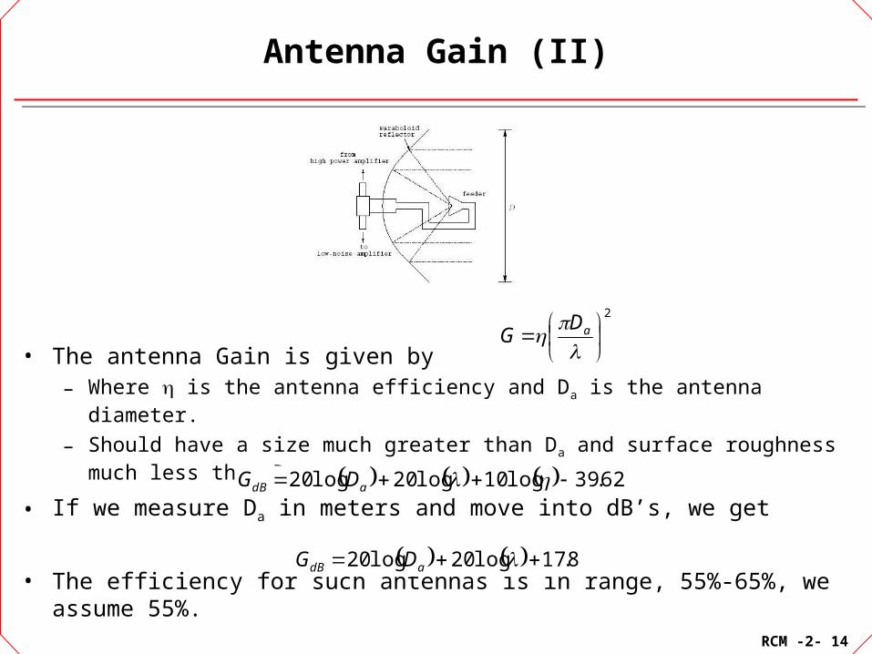
• The antenna Gain is given by– Where is the antenna efficiency and Da is the antenna diameter.
– Should have a size much greater than Da and surface roughness much less than Da.
• If we measure Da in meters and move into dB’s, we get
• The efficiency for such antennas is in range, 55%-65%, we assume 55%.
2
aDG
62.39log10log20log20 adB DG
8.17log20log20 adB DG
RCM -2- 15
Passive Repeaters
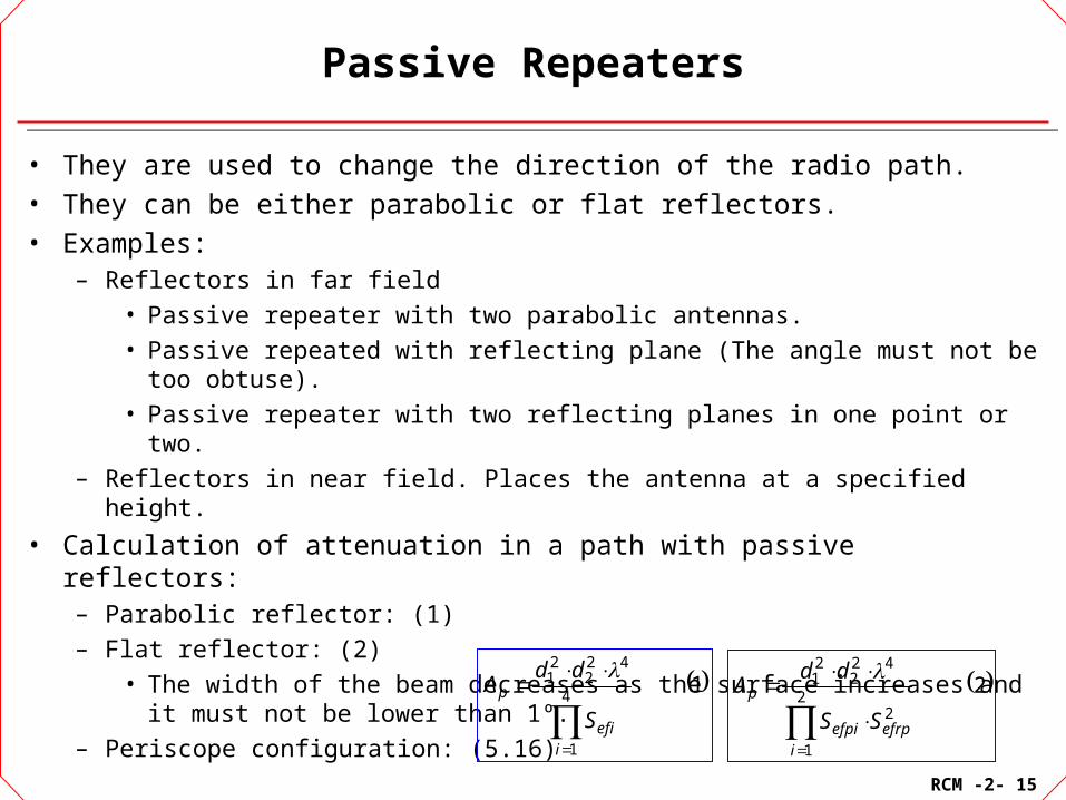
• They are used to change the direction of the radio path.
• They can be either parabolic or flat reflectors.
• Examples: – Reflectors in far field
• Passive repeater with two parabolic antennas.
• Passive repeated with reflecting plane (The angle must not be too obtuse).
• Passive repeater with two reflecting planes in one point or two.
– Reflectors in near field. Places the antenna at a specified height.
• Calculation of attenuation in a path with passive reflectors:– Parabolic reflector: (1)
– Flat reflector: (2)
• The width of the beam decreases as the surface increases and it must not be lower than 1º.
– Periscope configuration: (5.16) 14
1
422
21
iefi
p
S
ddA
22
2
1
422
21
efrpi
efpi
p
SS
ddA
RCM -2- 16
Fade Margin Calculation

RCM -2- 17
Other Random Processes
• In addition to the noise in the system that is seen as a random process, many other aspects of the system are subject to random processes.
• Many things are effecting the signals as they propagate.
• We cannot possibly know all the details of the environment through which the signal propagates, hence we have to model it by some degree of uncertainty.
• This randomness will have to be accounted for in both time and space.

RCM -2- 18
Calculating Fade Margins
• As stated, so far we have calculated only Free-space and atmospheric attenuation losses, but we have examined in detail the mechanisms that would lead to Fading.
• We have until now only spoken superficially about the effects of the fading in real terms, but have made it clear the amount of fade is a dynamic process.– This means that the changes in environment of weather conditions will cause changes in
the fade level through time.
– We have a calculated value for the signal strength presented to the receiver, RSL, but this is in fact a maximum value.
t
RSL
The RSL value for a path subject
to Free=space and atmospheric
attenuation only.
The real RSL value which
varies in time due to fading
processes.
RCM -2- 19
Statistical Nature Of Field Strength
• The complexity of the fading process and the number of parameters involved mean that we need to take a statistical view of the behaviour of the received field strength.
• The nature of the statistics is controlled by many factors. As stated before the terrain, climate and path length play a very significant role.
• Path lengths below 5 Kilometres can generally be regarded as fade free.
• We know that we have to obtained a specific level of C/N to actually receive the signal. This means in summary that to ensure the signal is received we need it to exceed a specific value which overcomes the thermal noise threshold.
• If the signal falls below this point the link can be considered to be non functioning.
• As the signal strength varies with time we can only ensure that the threshold is exceeded a certain percentage of the time.
RCM -2- 20
Outage Time
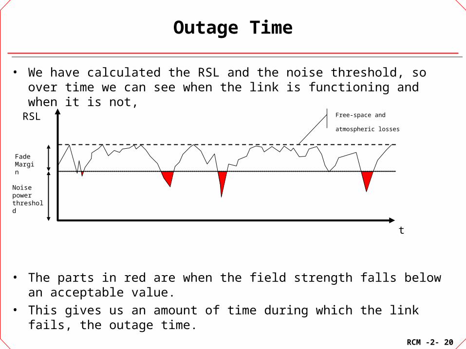
• We have calculated the RSL and the noise threshold, so over time we can see when the link is functioning and when it is not,
• The parts in red are when the field strength falls below an acceptable value.
• This gives us an amount of time during which the link fails, the outage time.
t
RSL Free-space and atmospheric
losses
Noise power threshold
Fade Margin

RCM -2- 21
Improving Outage Time
• We can design a particular RSLFS by increasing the transmission power, and/or the antenna gain etc.. Hence we can change the outage time by changing the RSL.
• In this case we have a much lower outage time, hence better performance.
• Of the many methods to support design, they are all effectively estimating the probable outage time for a limited set of input parameters.
t
RSL
Free-space and atmospheric
losses.
Noise power threshold
Fade Margin

RCM -2- 22
Using the Rayleigh Fading Assumptions
• Once you know what to calculate the trick is then to come up with a systematic method to do so.
• There are many models that are available and many organisations have come up with their own methodologies.
• The methods are based on finding the probability a field of a given strength will fall below a certain value for a known duration of time.
• If we assume that the fading is due entirely to multi-path conditions we can use the Rayleigh Distribution to calculate the worst fade conditions.
• The Rayleigh distribution in a microwave link is really a worst-case upper-bound value. Empirical measurements are also shown which indicate that other distributions are more appropriate, particularly over the shorter paths over land.
• As stated previously a complementary function can be defined that calculates the probability of exceeding a given value.

RCM -2- 23
Rayleigh Fade Margin (I)
• The graph shows the depth of fade in decibels versus the fractional time the fade is in excess of the abscissa.
• In summary this means if you take a point along the abscissa, say 25dB, then the graph tells you that the link would be down 0.003 fractional part of the time
• Additionally the graph shows three separate curves: a) The Rayleigh curve; b) the Durkee curve; and c) the curve used by the French P.T.T.
• This data is usually appropriate for a given type of terrain and climate and must be substituted when the conditions change.
RCM -2- 24
Rayleigh Fade Margin (II)
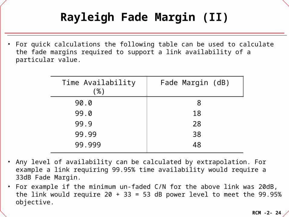
• For quick calculations the following table can be used to calculate the fade margins required to support a link availability of a particular value.
• Any level of availability can be calculated by extrapolation. For example a link requiring 99.95% time availability would require a 33dB Fade Margin.
• For example if the minimum un-faded C/N for the above link was 20dB, the link would require 20 + 33 = 53 dB power level to meet the 99.95% objective.
Time Availability (%) Fade Margin (dB)
90.0
99.0
99.9
99.99
99.999
8
18
28
38
48

RCM -2- 25
Path Classification Method (I)
• This method is based on CCIR recommendations and empirical results supplied by Siemens.
• Siemens has classified into three categories depending upon characteristics of the path.
• The method only applies to overland links that have unobstructed LOS conditions.

RCM -2- 26
Path Classification Method (II)
Type A These paths have favourable fading characteristics, troposphereic effects are rare. They are over hilly country, but not over wide river valleys and inland water; and in high mountainous country with paths hig above the valleys. They can also be characterised as being between a plain or a valley and mountains, where the angle of elevation exceeds 0.5o.
Type B These are paths with average fading characteristics and are typically over flat, or undulating country where troposphereic effects may occur. They are also over hilly country, but not over river valleys or open water. They are also characterised as being over coastal regions in moderate climates, but not over over the sea.
Type C These paths have adverse fading conditions. They are characterised as being over humid areas with ground fog being common. Paths that are low over flat country, such as wide river valleys and moors. They are typical of costal links in hot climates and paths in tropically regions with no angle of elevation.
RCM -2- 27
Path Classification Method (III)
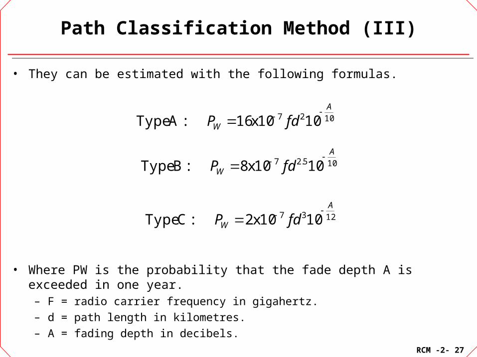
• They can be estimated with the following formulas.
• Where PW is the probability that the fade depth A is exceeded in one year.– F = radio carrier frequency in gigahertz.
– d = path length in kilometres.
– A = fading depth in decibels.
1027 1010x16:A TypeA
W fdP
105.27 1010x8:B TypeA
W fdP
1237 1010x2:C TypeA
W fdP

RCM -2- 28
ITU-R 530 Method
• This is a more sophisticated method and takes into account the type of terrain over which the link must travel.
• It introduces the concept of a geoclimatic factor K. Of which there are 4– Two types of K are used for over land links.
– Two types of K are used for over water links.

RCM -2- 29
Fading On Multi-Hop Paths
• Experimental evidence indicates that, in clear-air conditions, fading events exceeding 20 dB on adjacent hops in a multi-hop link are almost completely uncorrelated. This suggests that, for analogue systems with large fade margins, the outage time for a series of hops in tandem is approximately given by the sum of the outage times for the individual hops.
• For fade depths not exceeding 10 dB, the probability of simultaneously exceeding a given fade depth on two adjacent hops can be estimated from:
• where P1 and P2 are the probabilities of exceeding this fade depth on each individual hop (see Note).
• The correlation between fading on adjacent hops decreases with increasing fade depth between 10 and 20 dB, so that the probability of simultaneously exceeding a fade depth greater than 20 dB can be approximately expressed by:
• NOTE – The correlation between fading on adjacent hops is expected to be dependent on path length. The first Equation is an average based on the results of measurements on 47 pairs of adjacent line-of-sight hops operating in the 5 GHz band, with path lengths in the range of 11 to 97 km, and an average path length of approximately 45 km.
8.02112 )( PPP
2112 PPP

RCM -2- 30
Attenuation Due To Hydrometeors
• Attenuation can also occur as a result of absorption and scattering by such hydrometeors as rain, snow, hail and fog. Although rain attenuation can be ignored at frequencies below about 5 GHz, it must be included in design calculations at higher frequencies, where its importance increases rapidly. On paths at high latitudes or high altitude paths at lower latitudes, wet snow can cause significant attenuation over an even larger range of frequencies. More detailed information on attenuation due to hydrometeors other than rain is given in Recommendation ITU-R P.840.
• At frequencies where both rain attenuation and multipath fading must be taken into account, the exceedance percentages for a given fade depth corresponding to each of these mechanisms can be added.
RCM -2- 31
Techniques For Alleviating The Effects Of Multipath Propagation (I)
• The effects of slow relatively non-frequency selective fading (i.e. “flat fading”) due to beam spreading, and faster frequency-selective fading due to multipath propagation can be reduced by both non-diversity and diversity techniques.

RCM -2- 32
Techniques For Alleviating The Effects Of Multipath Propagation (II)
• Techniques without diversity: The guidance is divided into three groups: reduction of the levels of ground reflection, increase of path inclination, and reduction of path clearance.
– Reduction of ground reflection levels: Links should be sited where possible to reduce the level of surface reflections. Techniques include the siting of overwater links to place surface reflections on land rather than water and the siting of overland and overwater links to similarly avoid large flat highly reflecting surfaces on land. Another technique known to reduce the level of surface reflections is to tilt the antennas slightly upwards. Detailed information on appropriate tilt angles is not yet available. A trade-off must be made between the resultant loss in antenna directivity in normal refractive conditions that this technique entails, and the improvement in multipath fading conditions.
– Increase of path inclination Links should be sited to take advantage of terrain in ways that will increase the path inclination, since increasing path inclination is known to reduce the effects of beam spreading, surface multipath fading, and atmospheric multipath fading. The positions of the antennas on the radio link towers should be chosen to give the largest possible inclinations, particular for the longest links.
– Reduction of path clearance: Another technique that is less well understood involves the reduction of path clearance. A trade‑off must be made between the reduction of the effects of multipath fading and distortion and the increased fading due to sub-refraction. However, for the space diversity configuration one antenna might be positioned with low clearance.

RCM -2- 33
Space Diversity
TX
RX1
RX2
PROC
f1
f1
h

RCM -2- 34
Frequency Diversity
Señal de información Procesador
TX1 TX1
BR
RX1RX1
BR
f1
f2 f

RCM -2- 35
Techniques For Alleviating The Effects Of Multipath Propagation (III)
• Diversity techniques Diversity techniques include space, angle and frequency diversity. Frequency diversity should be avoided whenever possible so as to conserve spectrum. Whenever space diversity is used, angle diversity should also be employed by tilting the antennas at different upward angles. Angle diversity can be used in situations in which adequate space diversity is not possible or to reduce tower heights.
• The degree of improvement afforded by all of these techniques depends on the extent to which the signals in the diversity branches of the system are uncorrelated. For narrow-band analogue systems, it is sufficient to determine the improvement in the statistics of fade depth at a single frequency. For wideband digital systems, the diversity improvement also depends on the statistics of in-band distortion.
• The diversity improvement factor, I, for fade depth, A, is defined by:
I p( A ) / pd ( A )
• where pd (A) is the percentage of time in the combined diversity signal branch with fade depth larger than A and p(A) is the percentage for the unprotected path. The diversity improvement factor for digital systems is defined by the ratio of the exceedance times for a given BER with and without diversity.


