47
R&D White Paper WHP 031 July 2002 Reed-Solomon error correction C.K.P. Clarke Research & Development BRITISH BROADCASTING CORPORATION
| Date post: | 23-Apr-2018 |
| Category: |
Documents |
| Upload: | truongthuan |
| View: | 214 times |
| Download: | 0 times |
R&D White Paper
WHP 031
July 2002
Reed-Solomon error correction
C.K.P. Clarke
Research & Development BRITISH BROADCASTING CORPORATION


© BBC 2002. All rights reserved.
BBC Research & Development White Paper WHP 031
Reed-Solomon Error Correction
C. K. P. Clarke
Abstract
Reed-Solomon error correction has several applications in broadcasting, in particular forming part of the specification for the ETSI digital terrestrial television standard, known as DVB-T.
Hardware implementations of coders and decoders for Reed-Solomon error correction are complicated and require some knowledge of the theory of Galois fields on which they are based. This note describes the underlying mathematics and the algorithms used for coding and decoding, with particular emphasis on their realisation in logic circuits. Worked examples are provided to illustrate the processes involved.
Key words: digital television, error-correcting codes, DVB-T, hardware implementation, Galois field arithmetic


© BBC 2002. All rights reserved.
BBC Research & Development White Paper WHP 031
Reed-Solomon Error Correction
C. K. P. Clarke
Contents
1 Introduction ................................................................................................................................1 2 Background Theory....................................................................................................................2 2.1 Classification of Reed-Solomon codes ...................................................................................2 2.2 Galois fields ............................................................................................................................3 2.2.1 Galois field elements .........................................................................................................3 2.2.2 Galois field addition and subtraction.................................................................................3 2.2.3 The field generator polynomial .........................................................................................4 2.2.4 Constructing the Galois field.............................................................................................4 2.2.5 Galois field multiplication and division ............................................................................5
2.3 Constructing a Reed-Solomon code........................................................................................7 2.3.1 The code generator polynomial .........................................................................................7 2.3.2 Worked example based on a (15, 11) code........................................................................7 2.3.3 The code specified for DVB-T..........................................................................................8
3 Reed-Solomon Encoding............................................................................................................9 3.1 The encoding process..............................................................................................................9 3.1.1 The message polynomial ...................................................................................................9 3.1.2 Forming the code word....................................................................................................10 3.1.3 Basis for error correction.................................................................................................10
3.2 Encoding example.................................................................................................................10 3.2.1 Polynomial division.........................................................................................................11 3.2.2 Pipelined version .............................................................................................................12
3.3 Encoder hardware .................................................................................................................13 3.3.1 General arrangement .......................................................................................................13 3.3.2 Galois field adders...........................................................................................................13 3.3.3 Galois field constant multipliers......................................................................................13
3.3.3.1 Dedicated logic constant multipliers...........................................................................13 3.3.3.2 Look-up table constant multipliers .............................................................................14
3.4 Code shortening ....................................................................................................................15 4 Theory of error correction ........................................................................................................15 4.1 Introducing errors..................................................................................................................15 4.2 The syndromes ......................................................................................................................16

4.2.1 Calculating the syndromes ..............................................................................................16 4.2.2 Horner's method ..............................................................................................................16 4.2.3 Properties of the syndromes ............................................................................................16
4.3 The syndrome equations .......................................................................................................17 4.4 The error locator polynomial ................................................................................................17 4.5 Finding the coefficients of the error locator polynomial ......................................................18 4.5.1 The direct method............................................................................................................18 4.5.2 Berlekamp's algorithm.....................................................................................................18 4.5.3 The Euclidean algorithm .................................................................................................19
4.5.3.1 The syndrome polynomial ..........................................................................................19 4.5.3.2 The error magnitude polynomial.................................................................................19 4.5.3.3 The key equation.........................................................................................................19 4.5.3.4 Applying Euclid's method to the key equation ...........................................................19
4.6 Solving the error locator polynomial - the Chien search ......................................................20 4.7 Calculating the error values ..................................................................................................20 4.7.1 Direct calculation.............................................................................................................20 4.7.2 The Forney algorithm......................................................................................................20
4.7.2.1 The derivative of the error locator polynomial ...........................................................20 4.7.2.2 Forney's equation for the error magnitude ..................................................................21
4.8 Error correction .....................................................................................................................21 5 Reed-Solomon decoding techniques ........................................................................................21 5.1 Main units of a Reed-Solomon decoder................................................................................21 5.1.1 Including errors in the worked example..........................................................................22
5.2 Syndrome calculation............................................................................................................22 5.2.1 Worked examples for the (15, 11) code ..........................................................................22 5.2.2 Hardware for syndrome calculation ................................................................................24 5.2.3 Code shortening...............................................................................................................25
5.3 Forming the error location polynomial using the Euclidean algorithm................................25 5.3.1 Worked example of the Euclidean algorithm..................................................................25 5.3.2 Euclidean algorithm hardware.........................................................................................26
5.3.2.1 Full multipliers............................................................................................................28 5.3.2.2 Division or inversion...................................................................................................28
5.4 Solving the error locator polynomial - the Chien search ......................................................29 5.4.1 Worked example..............................................................................................................29 5.4.2 Hardware for polynomial solution...................................................................................30 5.4.3 Code shortening...............................................................................................................30
5.5 Calculating the error values ..................................................................................................31 5.5.1 Forney algorithm Example ..............................................................................................31 5.5.2 Error value hardware .......................................................................................................32
5.6 Error correction .....................................................................................................................32 5.6.1 Correction example .........................................................................................................32 5.6.2 Correction hardware ........................................................................................................33
5.7 Implementation complexity ..................................................................................................33 6 Conclusion................................................................................................................................33

7 References ................................................................................................................................33 8 Appendix ..................................................................................................................................34 8.1 Berlekamp's algorithm ..........................................................................................................34 8.1.1 The algorithm ..................................................................................................................34 8.1.2 Worked example..............................................................................................................35
8.2 Special cases in the Euclidean algorithm arithmetic.............................................................36 8.2.1 Single errors ....................................................................................................................36 8.2.2 Errors that make S3 zero ..................................................................................................37
8.3 Arithmetic look-up tables for the examples..........................................................................39

© BBC 2002. All rights reserved. Except as provided below, no part of this document may be reproduced in any material form (including photocopying or storing it in any medium by electronic means) without the prior written permission of BBC Research & Development except in accordance with the provisions of the (UK) Copyright, Designs and Patents Act 1988.
The BBC grants permission to individuals and organisations to make copies of the entire document (including this copyright notice) for their own internal use. No copies of this document may be published, distributed or made available to third parties whether by paper, electronic or other means without the BBC's prior written permission. Where necessary, third parties should be directed to the relevant page on BBC's website at http://www.bbc.co.uk/rd/pubs/whp for a copy of this document.
White Papers are distributed freely on request.
Authorisation of the Chief Scientist is required for publication.

1
BBC Research & Development
White Paper WHP 031
Reed-Solomon Error Correction
C. K. P. Clarke
1 Introduction Many digital signalling applications in broadcasting use Forward Error Correction, a technique in which redundant information is added to the signal to allow the receiver to detect and correct errors that may have occurred in transmission. Many different types of code have been devised for this purpose, but Reed-Solomon codes [1] have proved to be a good compromise between efficiency (the proportion of redundant information required) and complexity (the difficulty of coding and decoding). A particularly important use of a Reed-Solomon code for television applications is in the DVB-T transmission standard [2].
Hitherto, modulators and demodulators for DVB-T have, in general, used custom chips to provide the Reed-Solomon encoding and decoding functions. However, there are circumstances (such as for digital radio cameras) where it would be beneficial to include these processes in gate array designs for the transmitter and receiver. This would then provide the flexibility to modify the encoding parameters to suit the particular requirements of the radio camera application without sacrificing the compactness of single-chip implementation. Although custom core designs for gate arrays are available, the charges are significant and can complicate further exploitation of the intellectual property embodied in a design.
Although Reed-Solomon codes are described in many books on coding theory and have been the subject of many journal papers, the description of the hardware techniques involved is generally superficial, if described at all. The principal aim of this paper is to provide the basic information needed for the design of hardware implementations of Reed-Solomon coders and decoders, particularly those for the DVB-T system.
The mathematical basis for Reed-Solomon codes is complicated, but it is necessary to have a reasonable understanding of at least what needs to be done, if not why it is done. Therefore this paper first provides some essential background to the theory of Reed-Solomon codes and the Galois field arithmetic on which the codes are based. Then the process of encoding is described, first mathematically and then in terms of logic circuits. This is followed by an explanation of the basis of error correction and then by some of the decoding algorithms commonly applied in error correction hardware. Although some proofs are included, some results are just stated as a means of controlling the length of the document. At each stage, the techniques used are illustrated with worked examples.

2
2 Background Theory
2.1 Classification of Reed-Solomon codes There are many categories of error correcting codes, the main ones being block codes and convolutional codes. A Reed-Solomon code is a block code, meaning that the message to be transmitted is divided up into separate blocks of data. Each block then has parity protection information added to it to form a self-contained code word. It is also, as generally used, a systematic code, which means that the encoding process does not alter the message symbols and the protection symbols are added as a separate part of the block. This is shown diagrammatically in Figure 1.
code word (n symbols)
original message (k symbols)parity
(n-k=2t symbols)
symbol(m bits)
Figure 1 - Reed-Solomon code definitions
Also, a Reed-Solomon code is a linear code (adding two code words produces another code word) and it is cyclic (cyclically shifting the symbols of a code word produces another code word). It belongs to the family of Bose-Chaudhuri-Hocquenghem (BCH) codes [3, 4], but is distinguished by having multi-bit symbols. This makes the code particularly good at dealing with bursts of errors because, although a symbol may have all its bits in error, this counts as only one symbol error in terms of the correction capacity of the code.
Choosing different parameters for a code provides different levels of protection and affects the complexity of implementation. Thus a Reed-Solomon code can be described as an (n, k) code, where n is the block length in symbols and k is the number of information symbols in the message. Also
n ≤ 2m - 1 .... (1)
where m is the number of bits in a symbol. When (1) is not an equality, this is referred to as a shortened form of the code. There are n-k parity symbols and t symbol errors can be corrected in a block, where
t = (n-k)/2 for n-k even
or
t = (n-k-1)/2 for n-k odd.
Unfortunately, the notation used in the literature on error correcting codes, although generally similar, is not universally consistent. Although the notation used here is representative of that used elsewhere, the reader should be aware that confusing differences in terminology can arise. It is therefore particularly important to be clear about how the parameters of a code are specified.

3
2.2 Galois fields To proceed further requires some understanding of the theory of finite fields, otherwise known as Galois fields after the French mathematician.
2.2.1 Galois field elements A Galois field consists of a set of elements (numbers). The elements are based on a primitive element, usually denoted α, and take the values:
0, α0, α1, α2, .... , αN-1 .... (2)
to form a set of 2m elements, where N=2m - 1. The field is then known as GF(2m).
The value of α is usually chosen to be 2, although other values can be used. Having chosen α, higher powers can then be obtained by multiplying by α at each step. However, it should be noted that the rules of multiplication in a Galois field are not those that we might normally expect. This is explained in Section 2.2.5.
In addition to the powers of α form, shown in (2), each field element can also be represented by a polynomial expression of the form:
011
1 .... axaxa mm +++−
−
where the coefficients am-1 to a0 take the values 0 or 1. Thus we can describe a field element using the binary number am-1 .... a1a0 and the 2m field elements correspond to the 2m combinations of the m-bit number.
For example, in the Galois field with 16 elements (known as GF(16), so that m=4), the polynomial representation is:
00
11
22
33 xaxaxaxa +++
with a3a2a1a0 corresponding to the binary numbers 0000 to 1111. Alternatively, we can refer to the field elements by the decimal equivalents 0 to 15 as a short-hand version of the binary numbers.
Arithmetic in a finite field has processes of addition, subtraction, multiplication and division, but these differ from those we are used to with normal integers. The effect of these differences is that any arithmetic combination of field elements always produces another field element.
2.2.2 Galois field addition and subtraction When we add two field elements, we add the two polynomials:
00
11
11
00
11
11
00
11
11 ....)....()....( xcxcxcxbxbxbxaxaxa m
mm
mm
m +++=+++++++ −−
−−
−−
where
ci = ai + bi for 0 ≤ i ≤ m-1.
However, the coefficients can only take the values 0 and 1, so
ci = 0 for ai = bi
and
ci = 1 for ai ≠ bi .... (3)
Thus two Galois field elements are added by modulo-two addition of the coefficients, or in binary form, producing the bit-by-bit exclusive-OR function of the two binary numbers.

4
For example, in GF(16) we can add field elements x3 + x and x3 + x2 + 1 to produce x2 + x + 1. As binary numbers, this is:
1010 + 1101 = 0111
or as decimals
10 + 13 = 7
which can be seen from:
1010 (10) 1101 (13) 0111 (7) Because of the exclusive-OR function, the addition of any element to itself produces zero. So we should not be surprised that in a Galois field:
2 + 2 = 0.
Table 7 in Appendix 8.3 provides a look-up table for additions in GF(16).
Subtraction of two Galois field elements turns out to be exactly the same as addition because although the coefficients produced by subtracting the polynomials take the form:
ci = ai - bi for 0 ≤ i ≤ m-1
the resulting values for ci are the same as in (3). So, in this case, we get the more familiar result:
2 - 2 = 0
and for our other example:
10 - 13 = 7.
It is useful to realise that a field element can be added or subtracted with exactly the same effect, so minus signs can be replaced by plus signs in field element arithmetic.
2.2.3 The field generator polynomial An important part of the definition of a finite field, and therefore of a Reed-Solomon code, is the field generator polynomial or primitive polynomial, p(x). This is a polynomial of degree m which is irreducible, that is, a polynomial with no factors. It forms part of the process of multiplying two field elements together. For a Galois field of a particular size, there is sometimes a choice of suitable polynomials. Using a different field generator polynomial from that specified will produce incorrect results.
For GF(16), the polynomial
1)( 4 ++= xxxp .... (4)
is irreducible and therefore will be used in the following sections. An alternative which could have been used for GF(16) is
1)( 34 ++= xxxp .
2.2.4 Constructing the Galois field All the non-zero elements of the Galois field can be constructed by using the fact that the primitive element α is a root of the field generator polynomial, so that

5
p(α) = 0.
Thus, for GF(16) with the field generator polynomial shown in (4), we can write:
α4 + α + 1 = 0
or
α4 = α + 1 (remembering that + and − are the same in a Galois field).
Multiplying by α at each stage, using α + 1 to substitute for α4 and adding the resulting terms can be used to obtain the complete field as shown in Table 1. This shows the field element values in both index and polynomial forms along with the binary and decimal short-hand versions of the polynomial representation.
If the process shown in Table 1 is continued beyond α14, it is found that α15 = α0, α16 = α1, .... so that the sequence repeats with all the values remaining valid field elements.
index form
polynomial form
binary form
decimal form
0 0 0000 0 α0 1 0001 1 α1 α 0010 2 α2 α2 0100 4 α3 α3 1000 8 α4 α + 1 0011 3 α5 α2 + α 0110 6 α6 α3 + α2 1100 12 α7 α3 + α + 1 1011 11 α8 α2 + 1 0101 5 α9 α3 + α 1010 10 α10 α2 + α + 1 0111 7 α11 α3 + α2 + α 1110 14 α12 α3 + α2 + α + 1 1111 15 α13 α3 + α2 + 1 1101 13 α14 α3 + 1 1001 9
Table 1 - The field elements for GF(16) with p(x) = x4 + x + 1
2.2.5 Galois field multiplication and division Straightforward multiplication of two polynomials of degree m-1 results in a polynomial of degree 2m-2, which is therefore not a valid element of GF(2m). Thus multiplication in a Galois field is defined as the product modulo the field generator polynomial, p(x). The product modulo p(x) is obtained by dividing the product polynomial by p(x) and taking the remainder, which ensures that the result is always of degree m-1 or less and therefore a valid field element.
For example, if we multiply the values 10 and 13 from GF(16) represented by their polynomial expressions, we get:
xxxxxxxxxxxxxx
+++=+++++=+++
456
34356233 )1)(( .... (5)

6
To complete the multiplication, the result of (5) has to be divided by x4 + x + 1.
Division of one polynomial by another is similar to conventional long division. Thus it consists of multiplying the divisor by a value to make it the same degree as the dividend and then subtracting (which for field elements is the same as adding). This is repeated using the remainder at each stage until the terms of the dividend are exhausted. The quotient is then the series of values used to multiply the divisor at each stage plus any remainder left at the final stage.
This can be shown more easily by arranging the terms of the polynomials in columns according to their significance and then the calculation can be made on the basis of the coefficient values (0 or 1) as shown below.
x6 x5 x4 x3 x2 x1 x0 dividend: 1 1 1 0 0 1 0 divisor × x2: 1 0 0 1 1 1 1 1 1 1 divisor × x: 1 0 0 1 1 1 1 0 0 0 divisor × 1: 1 0 0 1 1 1 0 1 1 So the quotient is x2 + x + 1 and the remainder, which is the product of 10 and 13 that we were originally seeking, is x3 + x + 1 (binary 1011 or decimal 11). So we can write:
10 × 13 = 11.
Table 8 in Appendix 8.3 provides a look-up table for multiplications in GF(16) with the field generator polynomial of equation (4).
Alternatively the process of equation (5) can be performed using the coefficients of the polynomials in columns. First shifted versions of x3 + x are added according to the non-zero coefficients of x3 + x2 + 1. Then, instead of the division process, we can use substitutions taken from Table 1 for any non-zero terms that exceed the degree of the field elements and add these as shown:
x6 x5 x4 x3 x2 x1 x0 × x3: 1 0 1 0 × x2: 1 0 1 0 × 1: 1 0 1 0 1 1 1 0 0 1 0 x4 = x + 1 0 0 1 1 x5 = x2 + x 0 1 1 0 x6 = x3 + x2 1 1 0 0 1 0 1 1 A further alternative technique for multiplication in a Galois field, which is also convenient for division, is based on logarithms. If the two numbers to be multiplied are represented in index form, then the product can be obtained by adding the indices modulo 2m-1. For example, by inspecting the values in Table 1 we find:
10 = α9 and 13 = α13
so
10 × 13 = α9 × α13 = α(9+13)mod 15 = α(22)mod 15 = α7.
Again by inspection using Table 1 we find that:
α7 = 11

7
giving the result obtained by multiplying the polynomials.
A slight disadvantage of the logarithmic method is that field element 0 cannot be represented in index form. The method therefore has to sense the presence of zero values and force the result accordingly.
The logarithmic technique can also be used for division:
11 ÷ 10 = α7 ÷ α9 = α(7-9)mod 15 = α(-2)mod 15 = α13 = 13.
However, division of two field elements is often accomplished by multiplying by the inverse of the divisor. The inverse of a field element is defined as the element value that when multiplied by the field element produces a value of 1 (= α0). It is therefore possible to tabulate the inverse values of the field elements using Table 1.
For example, 10 = α9, so its inverse is α(-9)mod 15 = α6 = 12 from Table 1. So we can write:
11 ÷ 10 = 11 × 12
and then the product can be calculated by any of the methods above to be 13.
2.3 Constructing a Reed-Solomon code The values of the message and parity symbols of a Reed-Solomon code are elements of a Galois field. Thus for a code based on m-bit symbols, the Galois field has 2m elements.
2.3.1 The code generator polynomial An (n, k) Reed-Solomon code is constructed by forming the code generator polynomial g(x), consisting of n-k=2t factors, the roots of which are consecutive elements of the Galois field. Choosing consecutive elements ensures that the distance properties of the code are maximised. Thus the code generator polynomial takes the form:
))....()(()( 121 −++ +++= tbbb xxxxg ααα .... (6)
It should be noted that this expression is often quoted in the literature with subtle variations to catch the unwary. For example, the factors are often written as (x − αi), which emphasises that g(x) = 0 when x = αi and those familiar with Galois fields realise that − αi is exactly the same as αi. Also, some choose roots starting with α0 (b=0 in equation 6), while many others start with α, the primitive element (b=1 in equation 6). While each is valid, it results in a completely different code requiring changes in both the coder and decoder operation. If the chosen value of b is near 2m-1, then some of the roots may reach or exceed 12 −m
α . In this case the index values modulo 2m-1 can be substituted. Small reductions in the complexity of hardware implementations can result by choosing b=0, but this is not significant.
2.3.2 Worked example based on a (15, 11) code Specific examples are very helpful for obtaining a full understanding of the processes involved in Reed-Solomon coding and decoding. However, the (255, 239) code used in DVB-T is too unwieldy to be used for an example. In particular, the message length of several hundred symbols leads to polynomials with several hundred terms! In view of this, the much simpler (15, 11) code will be used to go through the full process of coding and decoding using methods that can be extended generally to other Reed-Solomon codes. Definition details of the (255, 239) code used for DVB-T are shown in Section 2.3.3.

8
For a (15, 11) code, the block length is 15 symbols, 11 of which are information symbols and the remaining 4 are parity words. Because t=2, the code can correct errors in up to 2 symbols in a block. Substituting for n in:
n = 2m - 1
gives the value of m as 4, so each symbol consists of a 4-bit word and the code is based on the Galois field with 16 elements. The example will use the field generator polynomial of equation (4), so that the arithmetic for the code will be based on the Galois field shown in Table 1.
The code generator polynomial for correcting up to 2 error words requires 4 consecutive elements of the field as roots, so we can choose:
g(x) = (x + α0) (x + α1) (x + α2) (x + α3)
= (x + 1) (x + 2) (x + 4) (x + 8)
using the index and decimal short-hand forms, respectively.
This expression has to be multiplied out to produce a polynomial in powers of x, which is done by multiplying the factors and adding together terms of the same order. As multiplication is easier in index form and addition is easier in polynomial form, the calculation involves repeatedly converting from one format to the other using Table 1. This is best done with a computer program for all but the simplest codes. Alternatively, we can take it factor by factor and use the look-up tables of Appendix 8.3 to give:
g(x) = (x + 1) (x + 2) (x + 4) (x + 8)
= (x2 + 3x + 2) (x + 4) (x + 8)
= (x3 + 7x2 + 14x + 8) (x + 8)
= x4 + 15x3 + 3x2 + x + 12 .... (7).
This can also be expressed as:
g(x) = α0x4 + α12x3 + α4x2 + α0x + α6
with the polynomial coefficients in index form.
2.3.3 The code specified for DVB-T The DVB-T standard [2] specifies a (255, 239, t=8) Reed-Solomon code, shortened to form a (204, 188, t=8) code, so that the 188 bytes of the input packet will be extended with 16 parity bytes to produce a coded block length of 204 symbols. For this code, the Galois field has 256 elements (m=8) and the polynomial representation of a field element is:
00
11
22
33
44
55
66
77 xaxaxaxaxaxaxaxa +++++++
corresponding to the binary numbers 00000000 to 11111111. Alternatively, we can use the decimal equivalents 0 to 255.
The specification also mentions the field generator polynomial, given as:
1)( 2348 ++++= xxxxxp .... (8).
This allows us to construct a table of field element values for GF(256) as shown in Table 2. This shows how the field element values can be built up row by row for the 256 element Galois field in a similar manner to the construction of Table 1. At each step the binary number representing the
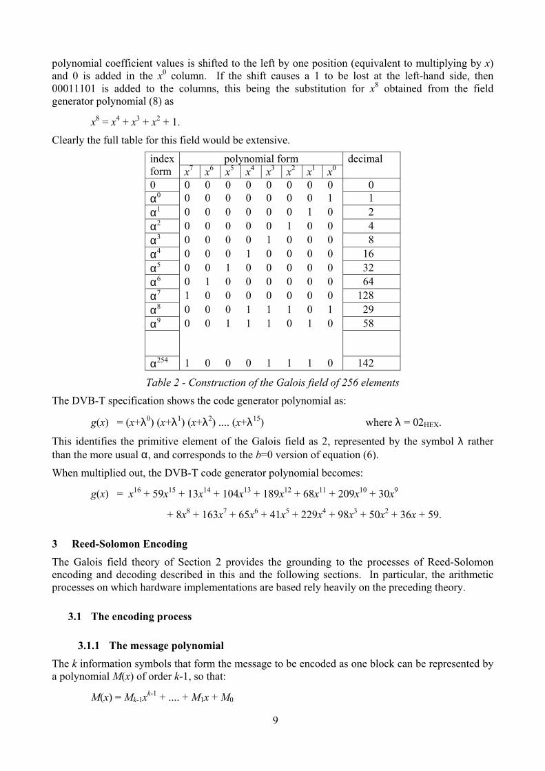
9
polynomial coefficient values is shifted to the left by one position (equivalent to multiplying by x) and 0 is added in the x0 column. If the shift causes a 1 to be lost at the left-hand side, then 00011101 is added to the columns, this being the substitution for x8 obtained from the field generator polynomial (8) as
x8 = x4 + x3 + x2 + 1.
Clearly the full table for this field would be extensive.
polynomial form index form x7 x6 x5 x4 x3 x2 x1 x0
decimal
0 0 0 0 0 0 0 0 0 0 α0 0 0 0 0 0 0 0 1 1 α1 0 0 0 0 0 0 1 0 2 α2 0 0 0 0 0 1 0 0 4 α3 0 0 0 0 1 0 0 0 8 α4 0 0 0 1 0 0 0 0 16 α5 0 0 1 0 0 0 0 0 32 α6 0 1 0 0 0 0 0 0 64 α7 1 0 0 0 0 0 0 0 128 α8 0 0 0 1 1 1 0 1 29 α9 0 0 1 1 1 0 1 0 58 α254 1 0 0 0 1 1 1 0 142
Table 2 - Construction of the Galois field of 256 elements
The DVB-T specification shows the code generator polynomial as:
g(x) = (x+λ0) (x+λ1) (x+λ2) .... (x+λ15) where λ = 02HEX.
This identifies the primitive element of the Galois field as 2, represented by the symbol λ rather than the more usual α, and corresponds to the b=0 version of equation (6).
When multiplied out, the DVB-T code generator polynomial becomes:
g(x) = x16 + 59x15 + 13x14 + 104x13 + 189x12 + 68x11 + 209x10 + 30x9
+ 8x8 + 163x7 + 65x6 + 41x5 + 229x4 + 98x3 + 50x2 + 36x + 59.
3 Reed-Solomon Encoding The Galois field theory of Section 2 provides the grounding to the processes of Reed-Solomon encoding and decoding described in this and the following sections. In particular, the arithmetic processes on which hardware implementations are based rely heavily on the preceding theory.
3.1 The encoding process
3.1.1 The message polynomial The k information symbols that form the message to be encoded as one block can be represented by a polynomial M(x) of order k-1, so that:
M(x) = Mk-1xk-1 + .... + M1x + M0
10
where each of the coefficients Mk-1, ...., M1, M0 is an m-bit message symbol, that is, an element of GF(2m). Mk-1 is the first symbol of the message.
3.1.2 Forming the code word To encode the message, the message polynomial is first multiplied by xn-k and the result divided by the generator polynomial, g(x). Division by g(x) produces a quotient q(x) and a remainder r(x), where r(x) is of degree up to n-k-1. Thus:
)()()(
)()(
xgxrxq
xgxxM kn
+=× −
.... (9)
Having produced r(x) by division, the transmitted code word T(x) can then be formed by combining M(x) and r(x) as follows:
T(x) = M(x) × xn-k + r(x)
= Mk-1xn-1 + .... + M0xn-k + rn-k-1xn-k-1 + .... + r0
which shows that the code word is produced in the required systematic form.
3.1.3 Basis for error correction Adding the remainder, r(x), ensures that the encoded message polynomial will always be divisible by the generator polynomial without remainder. This can be seen by multiplying equation (9) by g(x):
)()()()( xrxqxgxxM kn +×=× −
and rearranging:
)()()()( xqxgxrxxM kn ×=+× −
whereupon we note that the left-hand side is the transmitted code word, T(x), and that the right-hand side has g(x) as a factor. Also, because the generator polynomial, equation (6), has been chosen to consist of a number of factors, each of these is also a factor of the encoded message polynomial and will divide it without remainder. Thus, if this is not true for the received message, it is clear that one or more errors has occurred.
3.2 Encoding example We can now choose a message consisting of eleven 4-bit symbols for our (15, 11) code, for example, the values 1, 2, 3, 4, 5, 6, 7, 8, 9, 10, 11 which we wish to encode. These values are represented by a message polynomial:
x10 + 2x9 + 3x8 + 4x7 + 5x6 + 6x5 + 7x4 + 8x3 + 9x2 + 10x + 11 .... (10).
The message polynomial is then multiplied by x4 to give:
x14 + 2x13 + 3x12 + 4x11 + 5x10 + 6x9 + 7x8 + 8x7 + 9x6 + 10x5 + 11x4
to allow space for the four parity symbols. This polynomial is then divided by the code generator polynomial, equation (7), to produce the four parity symbols as a remainder. This can be accomplished in columns as a long division process as shown before, except that in this case, the coefficients of the polynomials are field elements of GF(16) instead of binary values, so the process is more complicated.

11
3.2.1 Polynomial division At each step the generator polynomial is multiplied by a factor, shown at the left-hand column, to make the most significant term the same as that of the remainder from the previous step. When subtracted (added), the most significant term disappears and a new remainder is formed. The 11 steps of the division process are as follows:
x14 x13 x12 x11 x10 x9 x8 x7 x6 x5 x4 x3 x2 x1 x0 1 2 3 4 5 6 7 8 9 10 11 0 0 0 0 × x10 1 15 3 1 12 13 0 5 9 6 × 13x9 13 7 4 13 3 7 1 4 5 7 × 7x8 7 11 9 7 2 10 13 2 5 8 × 10x7 10 12 13 10 1 1 15 15 9 9 × 1x6 1 15 3 1 12 0 12 8 5 10 × 0x5 0 0 0 0 0 12 8 5 10 11 × 12x4 12 8 7 12 15 0 2 6 4 0 × 0x3 0 0 0 0 0 2 6 4 0 0 × 2x2 2 13 6 2 11 11 2 2 11 0 × 11x 11 3 14 11 13 1 12 0 13 0 × 1 1 15 3 1 12 3 3 12 12
and the division produces the remainder:
r(x) = 3x3 + 3x2 + 12x + 12.
The quotient, q(x), produced as the left-hand column of multiplying values is not required and is discarded.
The encoded message polynomial T(x) is then:
x14 + 2x13 + 3x12 + 4x11 + 5x10 + 6x9 + 7x8 + 8x7
+ 9x6 + 10x5 + 11x4 + 3x3 + 3x2 + 12x + 12 .... (11)
or, written more simply:
1, 2, 3, 4, 5, 6, 7, 8, 9, 10, 11, 3, 3, 12, 12.

12
3.2.2 Pipelined version Hardware encoders usually operate on pipelined data, so the division calculation is made in a slightly altered form using the message bits one at a time as they are presented:
x14 x13 x12 x11 x10 x9 x8 x7 x6 x5 x4 x3 x2 x1 x0 0 0 0 0 1 g(x) × 1→ 15 3 1 12 15 3 1 12 2 g(x) × 13→ 7 4 13 3 4 5 1 3 3 g(x) × 7→ 11 9 7 2 14 8 4 2 4 g(x) × 10→12 13 10 1 4 9 8 1 5 g(x) × 1→ 15 3 1 12 6 11 0 12 6 g(x) × 0→ 0 0 0 0 11 0 12 0 7 g(x) × 12→ 8 7 12 15 8 11 12 15 8 g(x) × 0→ 0 0 0 0 11 12 15 0 9 g(x) × 2→ 13 6 2 11 1 9 2 11 10 g(x) × 11→ 3 14 11 13 10 12 0 13 0 11 g(x) × 1→ 15 3 1 12 3 3 12 12
With this arrangement, the first message value 1 is added to the contents of the most significant column, initially zero. The resulting value, 1, is then multiplied by the remaining coefficients of the generator polynomial 15, 3, 1, 12 to give the values to be added to the contents of the remaining columns, which are also initially zero. Then the second message value, 2, is added to the contents of the next most significant column, 15, to produce 13. This value is multiplied by the generator polynomial coefficients to give the values 7, 4, 13, and 3, and so on.

13
3.3 Encoder hardware
3.3.1 General arrangement The pipelined calculation shown in section 3.2.2 is performed using the conventional encoder circuit shown in Figure 2. All the data paths shown provide for 4-bit values.
D
input
D D D
1 1512 3
output
control
GFadder
GFmultiplier
KEY
Figure 2 - A (15, 11) Reed-Solomon encoder
During the message input period, the selector passes the input values directly to the output and the AND gate is enabled. After the eleven calculation steps shown above have been completed (in eleven consecutive clock periods) the remainder is contained in the D-type registers. The control waveform then changes so that the AND gate prevents further feedback to the multipliers and the four remainder symbol values are clocked out of the registers and routed to the output by the selector.
3.3.2 Galois field adders The adders of Figure 2 perform bit-by-bit addition modulo-2 of 4-bit numbers and each consists of four 2-input exclusive-OR gates. The multipliers, however, can be implemented in a number of different ways.
3.3.3 Galois field constant multipliers Since each of these units is multiplying by a constant value, one approach would be to use a full multiplier and to fix one input. Although a full multiplier is significantly more complicated, with an FPGA design, the logic synthesis process would strip out at least some of the unused circuitry. More will be said of full multipliers in Section 5.3.4.1. The other two approaches that come to mind are either to work out the equivalent logic circuit or to specify it as a look-up table, using a read-only memory.
3.3.3.1 Dedicated logic constant multipliers For the logic circuit approach, we can work out the required functionality by using a general polynomial representation of the input signal a3α3 + a2α2 + a1α + a0. This is then multiplied by the polynomials represented by the values 15, 3, 1 and 12 from Table 1. This involves producing a shifted version of the input for each non-zero coefficient of the multiplying polynomial. Where the shifted versions produce values in the α6, α5 or α4 columns, the 4-bit equivalents (from Table 1) are substituted. The bit values in each of the α3, α2, α1 and α0 columns are then added to give the required input bit contributions for each output bit.

14
For example, for multiplication by 15 (= α3 + α2 + α + 1):
α6 α5 α4 α3 α2 α1 α0 ×α3 a3 a2 a1 a0 0 0 0 ×α2 a3 a2 a1 a0 0 0 ×α a3 a2 a1 a0 0 ×1 a3 a2 a1 a0 a3 a2+a3 a1+a2+a3 0 0 a1+a2+a3 a1+a2+a3 0 a2+a3 a2+a3 0 a3 a3 0 0 a0+a1+a2 a0+a1 a0 a0+a1+a2+a3
The input bits contributing to a particular output bit are identified by the summation at the foot of each column. Similar calculations can be performed for multiplication by 3 (= α + 1), 1 (=1) and 12 (= α3 + α2) and give the results:
α3 α2 α1 α0 ×3 a2+a3 a1+a2 a0+a1+a3 a0+a3 ×1 a3 a2 a1 a0 ×12 a0+a1+a3 a0+a2 a1+a3 a1+a2 As the additions are modulo 2, these are implemented with exclusive-OR gates as shown in Figure 3.
a2
a1
a0
o2
o1
o0
a3 o3
multiply by 15
a2
a1
a0
o2
o1
o0
a3 o3
multiply by 3
a2
a1
a0
o2
o1
o0
a3 o3
a2
a1
a0
o2
o1
o0
a3 o3
multiply by 12multiply by 1
Figure 3 - Multipliers for the circuit of Figure 2
3.3.3.2 Look-up table constant multipliers Alternatively, each multiplier can be implemented as a look-up table with 2m = 16 entries. The entry values can be obtained by cyclically shifting the non-zero elements from Table 1 according to the index of the multiplication factor. This is because the multiplying index is added to the index of the input, modulo 15, thus shifting the results according to the multiplying value. However, the binary values of the polynomial coefficients of the input need to be arranged in ascending order to match the binary addressing of the look-up table memory. When this is done the values shown in Table 3 are produced.

15
input ×15 = α12 ×3 = α4 ×1 = α0 ×12 = α6 index form
decimal form
decimal form
decimal form
decimal form
decimal form
0 0 0 0 0 0 α0 1 15 3 1 12 α1 2 13 6 2 11 α4 3 2 5 3 7 α2 4 9 12 4 5 α8 5 6 15 5 9 α5 6 4 10 6 14 α10 7 11 9 7 2 α3 8 1 11 8 10 α14 9 14 8 9 6 α9 10 12 13 10 1 α7 11 3 14 11 13 α6 12 8 7 12 15 α13 13 7 4 13 3 α11 14 5 1 14 4 α12 15 10 2 15 8
Table 3 - Look-up tables for the fixed multipliers of Figure 2
3.4 Code shortening For a shortened version of the (15, 11) code, for example a (12, 8) code, the first three terms of the message polynomial, equation (10), would be set to zero. The effect of this on the pipelined calculation in section 3.2.2 is that all the columns would contain zero until the first non-zero input value associated with the x11 term. The calculation would then proceed as if it had been started at that point. Because of this, the circuit arrangement of Figure 2 can be used for the shortened code as long as the control waveform is high during the input data period, in this case eight clock periods instead of eleven.
4 Theory of error correction
4.1 Introducing errors Errors can be added to the coded message polynomial, T(x), in the form of an error polynomial, E(x). Thus the received polynomial, R(x), is given by:
R(x) = T(x) + E(x) .... (12)
where
E(x) = En-1xn-1 + .... + E1x + E0
and each of the coefficients En-1 .... E0 is an m-bit error value, represented by an element of GF(2m), with the positions of the errors in the code word being determined by the degree of x for that term. Clearly, if more than t = (n-k)/2 of the E values are non-zero, then the correction capacity of the code is exceeded and the errors are not correctable.

16
4.2 The syndromes
4.2.1 Calculating the syndromes In section 3.1.3 it was shown that the transmitted code word is always divisible by the generator polynomial without remainder and that this property extends to the individual factors of the generator polynomial. Therefore the first step in the decoding process is to divide the received polynomial by each of the factors (x + αi) of the generator polynomial, equation (6). This produces a quotient and a remainder, that is:
12)()( −+≤≤+
+=+
tbibforx
SxQx
xRi
iii αα
.... (13)
where b is chosen to match the set of consecutive factors in (6). The remainders Si resulting from these divisions are known as the syndromes and, for b=0, can be written as S0 .... S2t-1.
Rearranging (13) produces:
)()()( xRxxQS iii ++×= α
so that when x = αi this reduces to:
Si = R(αi)
= Rn-1(αi)n-1 + Rn-2(αi)n-2 + .... + R1αi + R0 .... (14)
where the coefficients Rn-1 .... R0 are the symbols of the received code word. This means that each of the syndrome values can also be obtained by substituting x = αi in the received polynomial, as an alternative to the division of R(x) by (x + αi) to form the remainder.
4.2.2 Horner's method Equation (14) can be re-written as:
Si = ( .... (Rn-1αi + Rn-2)αi + .... + R1)αi + R0
In this form, known as Horner's method, the process starts by multiplying the first coefficient Rn-1 by αi. Then each subsequent coefficient is added to the previous product and the resulting sum multiplied by αi until finally R0 is added. This has the advantage that the multiplication is always by the same value αi at each stage.
4.2.3 Properties of the syndromes Substituting in equation (12):
R(αi) = T(αi) + E(αi)
in which T(αi) = 0 because x+αi is a factor of g(x), which is a factor of T(x). So:
R(αi) = E(αi) = Si .... (15).
This means that the syndrome values are only dependent on the error pattern and are not affected by the data values. Also, when no errors have occurred, all the syndrome values are zero.
17
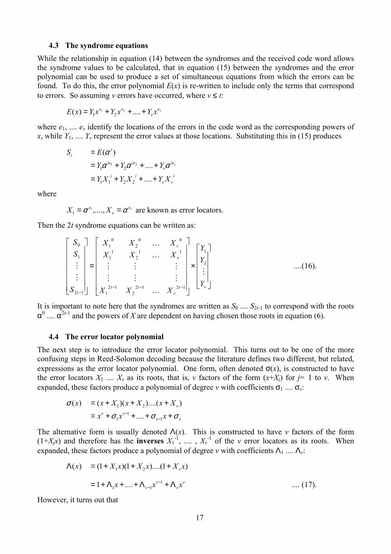
4.3 The syndrome equations While the relationship in equation (14) between the syndromes and the received code word allows the syndrome values to be calculated, that in equation (15) between the syndromes and the error polynomial can be used to produce a set of simultaneous equations from which the errors can be found. To do this, the error polynomial E(x) is re-written to include only the terms that correspond to errors. So assuming v errors have occurred, where v ≤ t:
vev
ee xYxYxYxE +++= ....)( 2121
where e1, .... ev identify the locations of the errors in the code word as the corresponding powers of x, while Y1, .... Yv represent the error values at those locations. Substituting this in (15) produces
ivv
ii
iev
ieie
ii
XYXYXY
YYY
ESv
+++=
+++=
=
....
....
)(
2211
2121 ααα
α
where
vev
e XX αα == ,....,11 are known as error locators.
Then the 2t syndrome equations can be written as:
×
=
−−−−
vtv
tt
v
v
t
Y
YY
XXX
XXXXXX
S
SS
M
K
MMM
MMM
K
K
M
M 2
1
12122
121
112
11
002
01
12
1
0
....(16).
It is important to note here that the syndromes are written as S0 .... S2t-1 to correspond with the roots α0 .... α2t-1 and the powers of X are dependent on having chosen those roots in equation (6).
4.4 The error locator polynomial The next step is to introduce the error locator polynomial. This turns out to be one of the more confusing steps in Reed-Solomon decoding because the literature defines two different, but related, expressions as the error locator polynomial. One form, often denoted σ(x), is constructed to have the error locators X1 .... Xv as its roots, that is, v factors of the form (x+Xj) for j= 1 to v. When expanded, these factors produce a polynomial of degree v with coefficients σ1 .... σv:
vvvv
v
xxx
XxXxXxx
σσσσ
++++=
+++=
−−
11
1
21
....
))....()(()(
The alternative form is usually denoted Λ(x). This is constructed to have v factors of the form (1+Xjx) and therefore has the inverses X1
-1, .... , Xv-1 of the v error locators as its roots. When
expanded, these factors produce a polynomial of degree v with coefficients Λ1 .... Λv:
)1)....(1)(1()( 21 xXxXxXx v+++=Λ
vv
vv xxx Λ+Λ++Λ+= −−
111 ....1 .... (17).
However, it turns out that
18
Λ× =
xxx v 1)(σ
so the coefficients σ1 .... σv are the same as Λ1 .... Λv.
4.5 Finding the coefficients of the error locator polynomial
4.5.1 The direct method
For each error, there is a corresponding root Xj-1 that makes Λ(x) equal to zero. So
0....1 11
11 =Λ+Λ++Λ+ −+−
−− v
jvv
jvj XXX
or multiplied through by YjXji+v:
0.... 11
11 =Λ+Λ++Λ+ +
−−++ i
jjvi
jjvvi
jjvi
jj XYXYXYXY .
Similar equations can be produced for all the errors (different values of j) and the terms collected so that:
∑∑∑==
−+
=
+ =Λ++Λ+v
j
ijj
v
jv
vijj
v
j
vijj XYXYXY
11
1
11 0....
or
0....11 =Λ++Λ+ −++ ivvivi SSS
recognising that the summation terms are the syndrome values using (16). Similar equations can be derived for other values of i so that:
0....11 =Λ++Λ+ −++ ivvivi SSS for i = 0, .... , 2t-v-1 .... (18)
so producing a set of 2t-v simultaneous equations, sometimes referred to as the key equations, with Λ1 .... Λv as unknowns.
To solve this set of equations for Λ1 .... Λv, we can use the first v equations, represented by the matrix equation (19), except that, at this point, v is unknown:
Λ
ΛΛΛ
×
=
−−−−
−+
−−
−−−
−
+
+
vvvvv
vvv
vvv
vvv
v
v
v
v
SSSS
SSSSSSSSSSSS
S
SSS
M
L
MMMM
L
L
L
M3
2
1
1423222
211
121
0321
12
2
1
.... (19).
Because of this, it is necessary to calculate the determinant of the matrix for each value of v, starting at v=t and working down, until a non-zero determinant is found. This indicates that the equations are independent and can be solved. The coefficients of the error locator polynomial Λ1 .... Λv can then be found by inverting the matrix to solve the equations.
4.5.2 Berlekamp's algorithm Berlekamp's algorithm [5, 6] is a more efficient iterative technique of solving equations (18) that also overcomes the problem of not knowing v. This is done by forming an approximation to the error locator polynomial, starting with Λ(x)=1. Then at each stage, an error value is formed by
19
substituting the approximate coefficients into the equations corresponding to that value of v. The error is then used to refine a correction polynomial, which is then added to improve the approximate Λ(x). The process ends when the approximate error locator polynomial checks consistently with the remaining equations. A statement of the algorithm and a worked example is included in the Appendix as Section 8.1.
4.5.3 The Euclidean algorithm Another efficient technique for obtaining the coefficients of the error location polynomial is based on Euclid's method for finding the highest common factor of two numbers [7]. This uses the relationship between the errors and the syndromes expressed in the form of an equation based on polynomials. This is also often referred to as the fundamental or key equation and requires two new polynomials, the syndrome and error magnitude polynomials, to be introduced.
4.5.3.1 The syndrome polynomial For use in the key equation, the syndrome polynomial is defined as:
S(x) = Sb+2t-1x2t-1 + .... + Sb+1x + Sb
where the coefficients are the 2t syndrome values calculated from the received code word using equation (14), or its equivalent for other values of b.
4.5.3.2 The error magnitude polynomial The error magnitude polynomial can be written as:
Ω(x) = Ωv-1xv-1 + .... + Ω1x + Ω0
This is sometimes referred to as the error value or error evaluator polynomial.
4.5.3.3 The key equation The key equation can then be written as:
Ω(x) = [S(x) Λ(x)] mod x2t
where S(x) is the syndrome polynomial and Λ(x) is the error locator polynomial. Any terms of degree x2t or higher in the product are ignored, so that
Ω0 = Sb
Ω1 = Sb+1 + SbΛ1
M
Ωv-1 = Sb+v-1 + Sb+v-2Λ1 + .... + SbΛv-1
4.5.3.4 Applying Euclid's method to the key equation Euclid's method [7] can find the highest common factor d of two elements a and b, such that:
ua + vb = d .... (20)
where u and v are coefficients produced by the algorithm.
The product of S(x), which has degree 2t-1, and Λ(x), which has degree v, will have degree 2t+v-1. So the product can be expressed as:

20
S(x) × Λ(x) = F(x) × x2t + Ω(x)
in which the terms of x2t and above are represented by the F(x) term and the remaining part is represented by Ω(x). This can be rearranged as:
Λ(x) × S(x) + F(x) × x2t = Ω(x)
so that the known terms S(x) and x2t correspond to the a and b terms of (20). The algorithm then consists of dividing x2t by S(x) to produce a remainder. S(x) then becomes the dividend and the remainder becomes the divisor to produce a new remainder. This process is continued until the degree of the remainder becomes less than t. At this point, both the remainder Ω(x) and the multiplying factor Λ(x) are available as terms in the calculation.
4.6 Solving the error locator polynomial - the Chien search
Having calculated the coefficient values, Λ1 .... Λv, of the error locator polynomial, it is now possible to find its roots. If the polynomial is written in the form:
Λ(x) = X1(x + X1-1) X2(x + X2
-1) ....
then clearly the function value will be zero if x = X1-1, X2
-1, .... , that is:
,...., 21 eex −−= αα .
The roots, and hence the values of X1 .... Xv, are found by trial and error, known as the Chien search [8], in which all the possible values of the roots (the field values αi, 0 ≤ i ≤ n-1) are substituted into equation (17) and the results evaluated. If the expression reduces to zero, then that value of x is a root and identifies the error position. Since the first symbol of the code word corresponds to the xn-1 term, the search begins with the value α-(n-1) (=α1), then α-(n-2) (=α2), and continues to α0, which corresponds to the last symbol of the code word.
4.7 Calculating the error values
4.7.1 Direct calculation When the error locations X1 .... Xv are substituted into the syndrome equations (16), the first v equations can be solved by matrix inversion to produce the error values Y1 .... Yv.
4.7.2 The Forney algorithm This is an alternative means of calculating the error value Yj having established the error locator polynomial Λ(x) and the error value polynomial Ω(x). If Berlekamp's algorithm has been used to find Λ(x), then Ω(x) can be found by using the relationships in Section 4.5.3.3. The algorithm makes use of the derivative of the error locator polynomial.
4.7.2.1 The derivative of the error locator polynomial For a polynomial f(x) given by:
f(x) = 1 + f1x + f2x2 + .... + fvxv
the derivative is given by:
f '(x) = f1 + 2f2x + .... + vfvxv-1
However, for the error locator polynomial Λ(x), for x = Xj-1, the derivative reduces to:

21
Λ'(Xj-1) = Λ1 + Λ3Xj
-2 + Λ5Xj-4 + ....
which amounts to setting even-powered terms of the error locator polynomial to zero and dividing through by x = Xj
-1.
4.7.2.2 Forney's equation for the error magnitude Methods of calculating the error values Y1 .... Yv based on Forney's algorithm are more efficient than the direct method of solving the syndrome equations as described in section 4.7.1. According to Forney's algorithm, the error value is given by:
)(')(
1
11
−
−−
ΛΩ
=j
jbjj X
XXY ....(21)
where Λ'(Xj-1) is the derivative of Λ(x) for x = Xj
-1. When b=1, the Xj1-b term disappears, so the
formula is often quoted in the literature as simply Ω/Λ', which gives the wrong results for b=0 and other values. (The value of b is defined in equation (6).)
It should be noted that equation (21) only gives valid results for symbol positions containing an error. If the calculation is made at other positions, the result is generally non-zero and invalid. The Chien search is therefore still needed to identify the error positions.
4.8 Error correction Having located the symbols containing errors, identified by Xj, and calculated the values Yj of those errors, the errors can be corrected by adding the error polynomial E(x) to the received polynomial R(x). It should be remembered that conventionally the highest degree term of the received polynomial corresponds to the first symbol of the received code word.
5 Reed-Solomon decoding techniques Whereas the previous section has dealt with the underlying theory and, in some cases, identified several alternative approaches to some processes, this section will describe a specific approach to decoding hardware based around the Euclidean algorithm.
5.1 Main units of a Reed-Solomon decoder The arrangement of the main units of a Reed-Solomon decoder reflects, for the most part, the processes of the previous Section.
inputR
calculate thesyndromes
output
Chien searchfor errorpositions
form theerror locationpolynomial:
Euclid
calculate theerror values:
Forney method
data delay
SΩ, Λ'
Λ
Ω/Λ' Y
X
Figure 4 - Main processes of a Reed-Solomon decoder

22
Thus, in Figure 4, the first process is to calculate the syndrome values from the incoming code word. These are then used to find the coefficients of the error locator polynomial Λ1 .... Λv and the error value polynomial Ω0 .... Ωv-1 using the Euclidean algorithm. The error locations are identified by the Chien search and the error values are calculated using Forney's method. As these calculations involve all the symbols of the received code word, it is necessary to store the message until the results of the calculation are available. Then, to correct the errors, each error value is added (modulo 2) to the symbol at the appropriate location in the received code word.
5.1.1 Including errors in the worked example. The steps in the decoding process are illustrated by continuing the worked example of the (15, 11) Reed-Solomon code that was used with the encoding process in Section 3.
Introducing two errors in the sixth (x9 term) and thirteenth (x2 term) symbols of the coded message produces an error polynomial with two non-zero terms:
E(x) = E9x9 + E2x2
and we can choose, for example, E9 = 13 and E2 = 2, so that three bits of the sixth symbol are altered while only one bit of the thirteenth symbol is affected. Although there are four bits in error, in terms of the error correcting capacity of the code this constitutes only two errors because this is based on the number of symbols in error. Therefore these errors should be correctable.
Addition of the errors makes the received message:
R(x) = (x14 + 2x13 + 3x12 + 4x11 + 5x10 + 6x9 + 7x8 + 8x7
+ 9x6 + 10x5 + 11x4 + 3x3 + 3x2 + 12x + 12) + (13x9 + 2x2)
= x14 + 2x13 + 3x12 + 4x11 + 5x10 + 11x9 + 7x8 + 8x7
+ 9x6 + 10x5 + 11x4 + 3x3 + x2 + 12x + 12 .... (22)
or, more simply
1, 2, 3, 4, 5, 11, 7, 8, 9, 10, 11, 3, 1, 12, 12.
5.2 Syndrome calculation
5.2.1 Worked examples for the (15, 11) code
Section 4.2 showed that the syndrome corresponding to each root αi of the generator polynomial could be calculated either by dividing the received polynomial R(x) by x + αi, or by evaluating R(αi). In the latter case, Horner's method proves an efficient technique.
For the direct division process, we would use a method of calculation similar to that of Section 3.2.1. However, the pipelined approach of Section 3.2.2 is more suitable for hardware, so the calculation of S0, corresponding to root α0, consists of the following steps where, in this case, the multiplication by α0 (= 1) is trivial:

23
x14 x13 x12 x11 x10 x9 x8 x7 x6 x5 x4 x3 x2 x1 x0 0 R14 1 α0 × 1→ 1 R13 2 α0 × 3→ 3 R12 3 α0 × 0→ 0 R11 4 α0 × 4→ 4 R10 5 α0 × 1→ 1 R9 11 α0 × 10→ 10 R8 7 α0 × 13→ 13 R7 8 α0 × 5→ 5 R6 9 α0 × 12→ 12 R5 10 α0 × 6→ 6 R4 11 α0 × 13→ 13 R3 3 α0 × 14→ 14 R2 1 α0 × 15→ 15 R1 12 α0 × 3→ 3 R0 12 15 giving
S0 = 15.
Alternatively, we can use substitution of the root value in equation (22), so for S1, substituting α1 for x and using the equivalences of Table 1, we obtain:
S1 = (α1)14 + 2(α1)13 + 3(α1)12 + 4(α1)11 + 5(α1)10 + 11(α1)9 + 7(α1)8 + 8(α1)7
+ 9(α1)6 + 10(α1)5 + 11(α1)4 + 3(α1)3 + (α1)2 + 12(α1) + 12
= 3
Or if we use Horner's method:
S2 = (((((((((((((1 × α2 + 2) × α2 + 3) × α2 + 4) × α2 + 5) × α2 + 11) ×
α2 + 7) × α2 + 8) × α2 + 9) × α2 + 10) × α2 + 11) × α2 + 3) ×
α2 + 1) × α2 + 12) × α2 + 12
= 4

24
Alternatively Horner's method can be written as a series of intermediate steps. So, for S3 where α3 = 8:
( 0 + 1 ) × 8 = 8( 8 + 2 ) × 8 = 15( 15 + 3 ) × 8 = 10( 10 + 4 ) × 8 = 9( 9 + 5 ) × 8 = 10( 10 + 11 ) × 8 = 8( 8 + 7 ) × 8 = 1( 1 + 8 ) × 8 = 4( 4 + 9 ) × 8 = 2( 2 + 10 ) × 8 = 12( 12 + 11 ) × 8 = 13( 13 + 3 ) × 8 = 9( 9 + 1 ) × 8 = 12( 12 + 12 ) × 8 = 0 0 + 12 = 12
so that
S3 = 12.
5.2.2 Hardware for syndrome calculation The hardware arrangement used for syndrome calculation, shown in Figure 5, can be interpreted either as a pipelined polynomial division or as an implementation of Horner's method.
input
D
αi
Si
control
Figure 5 - Forming a syndrome
In the case of polynomial division, the process is basically the same as that described for encoding in section 3.2.2 (and shown in Figure 2), except much simpler because the degree of the divisor polynomial is one. Thus there is only one feedback term with one multiplier, multiplying by αi, and only one register. As before, the input values are added to the output of the register and all the data paths are m-bit signals. The only difference in this case is that the AND-gate is used to prevent the contents of the register contributing at the start of the code word, which was achieved in Figure 2 by clearing the registers at the start of each block.
Alternatively, this circuit can be seen as a direct implementation of Horner's method, in which the incoming symbol value is added to the contents of the register before being multiplied by αi and the result returned to the register.
Clearly, all n symbols of the code word have to be accumulated before the syndrome value is produced. Also, 2t circuits of the form of Figure 5 are required, one for each value of αi, each

25
corresponding to a root of the generator polynomial. The Galois field adders and fixed multipliers can be implemented using the techniques described in Sections 3.3.2 and 3.3.3.
5.2.3 Code shortening If the code is used in a shortened form, such as with a (12, 8) code as described in Section 3.4, then the first part of the message is not present. Thus the pipelined calculation need only begin when the first element of the shortened message is present. The same arrangement can therefore be used for the shortened code provided that the AND gate is controlled to prevent the register contents contributing to the first addition.
5.3 Forming the error location polynomial using the Euclidean algorithm
5.3.1 Worked example of the Euclidean algorithm To continue the worked example to find the coefficients of the error locator polynomial, it is first necessary to form the syndrome polynomial. The syndrome values obtained in Section 5.2.1 are:
S0 = 15, S1 = 3, S2 = 4 and S3 = 12
so the syndrome polynomial is:
S(x) = S3x3 + S2x2 + S1x + S0
= 12x3 + 4x2 + 3x + 15
The first step of the algorithm (described in Section 4.5.3.4) is to divide x2t (in this case x4) by S(x). This involves multiplying S(x) × 10x (10 = 1/12) and subtracting (adding), followed by S(x) × 6 (6 = 14/12) and subtracting. This gives the remainder 6x2 + 6x + 4. In the right hand process, the initial value 1 is multiplied by the same values used in the division process and added to an initial sum value of zero. So the right-hand calculation produces 0 + 1 × (10x + 6) = 10x + 6.
x4 x3 x2 x1 x0 x2 x1 x0 dividend: 1 0 0 0 0 0 0 divisor × 10x: 1 14 13 12 10 0 14 13 12 0 10 0 divisor × 6: 14 11 10 4 0 6 remainder: 6 6 4 10 6
Having completed the first division, the degree of the remainder is not less than t (= 2), so we do a new division using the previous divisor as the dividend and the remainder as the divisor, that is, dividing S(x) by the remainder 6x2 + 6x + 4. First the remainder is multiplied by 2x (2 = 12/6) and subtracted, then multiplied by 13 (13 = 8/6) and subtracted to produce the remainder 3x + 14. At the right hand side, the previous initial value (1) becomes the initial sum value and the previous result (10x + 6) is multiplied by the values used in the division process. This produces 1 + (10x + 6) × (2x + 13) = 7x2 + 7x + 9.
x4 x3 x2 x1 x0 x2 x1 x0 dividend: 12 4 3 15 0 1 divisor × 2x: 12 12 8 7 12 0 8 11 15 7 12 1 divisor × 13: 8 8 1 11 8 remainder: 3 14 7 7 9

26
In general, the process would continue repeating the steps described above, but now the degree of the remainder (= 1) is less than t (= 2) so the process is complete. The two results 7x2 + 7x + 9 and 3x + 14 are in fact γ×Λ(x) and γ×Ω(x), respectively, where in this case the constant factor γ=9. So dividing through by 9 gives the polynomials in the defined forms:
Λ(x) = 14x2 + 14x + 1
and
Ω(x) = 6x + 15.
Further examples of the Euclidean algorithm, which result in somewhat different sequences of operations, are shown in Appendix 8.2.
5.3.2 Euclidean algorithm hardware The Euclidean algorithm can be performed using the arrangement of Figure 6 in which all data paths are 4 bits wide. This arrangement broadly follows the calculation of Section 5.3.1 so that the lower part of the diagram performs the division (the left-hand side of the calculation) while the upper part performs the multiplication (the right-hand side). Initially, the B register is loaded to contain the dividend and the A register to contain the syndrome values. Also, the C register is set to 1 and the D register, set to the initial sum, zero.
At each step, the contents of B3 is divided by A3 (that is, multiplied by the inverse of A3) and the result used in the remaining multipliers. The results of the multiplications are then added to the contents of the B and D registers to form the intermediate results. At step one, the results are loaded back into the B and D registers and the contents of the A and C registers are retained. At step two, the contents of the A and C registers are transferred to the B and D registers and the calculation results are loaded into the A and C registers. Where necessary, the values are shifted between registers of different significance to take account of multiplications by x. Table 4 shows the contents of the registers at intermediate steps in the calculation.
step A3 A2 A1 A0 B3 B2 B1 B0 C1 C0 D2 D1 D0 1 12 4 3 15 1 0 0 0 0 1 0 0 0 2 12 4 3 15 14 13 12 0 0 1 0 10 0 3 6 6 4 0 12 4 3 15 10 6 0 0 1 4 6 6 4 0 8 11 15 0 10 6 7 12 1
Table 4 - Register contents in the calculation of Section 5.3.1
It should be noted that Figure 6 represents a simplification of the process and, as shown, will not produce the correct results for some error patterns. This occurs when the contents of A3 is zero, potentially resulting in division by zero. Some examples of this are shown in the Appendix, Section 8.2. Additional circuitry is required to sense these conditions and to alter the calculation sequence of Figure 6 accordingly.
A further point is that the Λ and Ω outputs produced when the calculation is complete do not include the final division shown in 5.3.1. Thus these values are multiplied by a constant (γ) relative to their defined values.
The arrangement of Figure 6 shows the Euclidean algorithm in a highly parallel form and there is considerable scope for reducing the hardware requirements by re-using circuit elements, particularly the multipliers. A commonly used arrangement is to recognise that the upper and lower circuits of Figure 6 are very similar. Because of this, it is possible to use one circuit with duplicated registers and to interleave the steps of the calculation accordingly.

27
D0
S0
inv
shift
S1
S2
S3
0
0
0
1
0
0
0
0
1
0
γ
γΛ1
γΛ2
γΩ0
γΩ1
0
0
D1
D2
C0
C1
B0
B1
B2
B3
A0
A1
A2
A3
Figure 6 - The Euclidean processor

28
5.3.2.1 Full multipliers The Galois field multipliers described up to this point have involved multiplication by a constant, whereas those of Figure 6 are full multipliers. Full multipliers can be implemented by similar techniques to those described in Section 3.3.3, either as dedicated logic multipliers or as look-up tables, although with 22m locations, the latter technique rapidly becomes inefficient as the value of m increases. It is also possible to use look-up tables with 2m locations to convert to logarithms, which can then be added modulo 2m - 1 and the result converted back with an inverse look-up table. The need to sense zero inputs and produce a modulo 2m - 1 result generally makes this technique more complicated than the shift-and-add approach.
a2
a1
a0
a3
o2
o1
o0
o3
b2
b1
b0
b3
Figure 7 - A full multiplier for GF(16)
Figure 7 shows the arrangement of a 4-bit by 4-bit shift-and-add multiplier, drawn to emphasise the three underlying processes. First the array of AND gates generates the set of shifted product terms, producing seven levels of significance. Next the first column of exclusive-OR gates sums (modulo 2) the products at each level. Finally, the three upper levels beyond the range of field values are converted to fall within the field, using the relationships of Table 1, and the contributions added by the three pairs of exclusive-OR gates.
5.3.2.2 Division or inversion Having designed a multiplier, then it is probably most straightforward to implement Galois field division using a look-up table with 2m locations to generate the inverse and then to multiply. The inverses are easily calculated as shown in Table 5 using field elements in index form. This shows the element values in ascending order to correspond with the addressing of the look-up table.

29
input (decimal)
input (index)
inverse (index)
inverse (decimal)
0 0 0 0 1 α0 α0 1 2 α1 α-1 = α14 9 3 α4 α-4 = α11 14 4 α2 α-2 = α13 13 5 α8 α-8 = α7 11 6 α5 α-5 = α10 7 7 α10 α-10 = α5 6 8 α3 α-3 = α12 15 9 α14 α-14 = α1 2 10 α9 α-9 = α6 12 11 α7 α-7 = α8 5 12 α6 α-6 = α9 10 13 α13 α-13 = α2 4 14 α11 α-11 = α4 3 15 α12 α-12 = α3 8
Table 5 - Look-up table for inverse values in GF(16)
The table includes 0 as the Galois field inverse of 0.
5.4 Solving the error locator polynomial - the Chien search
5.4.1 Worked example
To try the first position in the code word, corresponding to ej=14, we need to substitute α-14 into the error locator polynomial:
Λ(x) = 14x2 + 14x + 1
Λ(α-14) = 14(α-14)2 + 14(α-14) + 1
= 14(α1)2 + 14(α1) + 1
= α11 α2 + α11 α1 + α0
= α13 + α12 + α0
= 13 + 15 + 1
= 3
and the non-zero result shows that the first position does not contain an error.
For subsequent positions, the power of α to be substituted will advance by one for the x term and by two for the x2 term, so we can tabulate the calculations as shown in Table 6.

30
x x2 term x term unity sum α-14 α13 α12 1 3 α-13 α0 α13 1 13 α-12 α2 α14 1 12 α-11 α4 α0 1 3 α-10 α6 α1 1 15 α-9 α8 α2 1 0 α-8 α10 α3 1 14 α-7 α12 α4 1 13 α-6 α14 α5 1 14 α-5 α1 α6 1 15 α-4 α3 α7 1 2 α-3 α5 α8 1 2 α-2 α7 α9 1 0 α-1 α9 α10 1 12 α0 α11 α11 1 1
Table 6 - Terms in the Chien search example
Having derived the values for the first row (multiplying Λ2 by α2 and Λ1 by α), each new row can be obtained from the previous row in the same way. Adding the terms together then produces the sum for each row. The two sum values of zero in Table 6 identify the error positions correctly as the 6th and 13th symbols, corresponding to the x9 and x2 terms, respectively, of the code word polynomial.
Checking these results by multiplying out the factors, we obtain:
(α9x + 1)(α2x + 1) = α11x2 + (α9 + α2)x + 1
= 14x2 + 14x + 1 = Λ(x) as before.
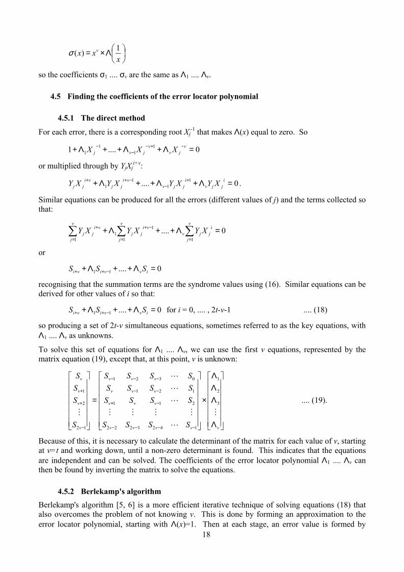
5.4.2 Hardware for polynomial solution The calculations of Table 6 form the basis of the method used to find the roots of the error locator polynomial shown in Figure 8. The value of each term in the polynomial is calculated by loading the coefficient value γΛ and multiplying it by the appropriate power of α. Then at each successive clock period, the next value of the term is produced by multiplying the previous result by the power of α. Adding the values of the individual terms together produces the value of the polynomial for each symbol position in turn. Detecting zero values of the sum identifies symbol positions containing errors and is not affected by the presence of the multiplying factor γ.
It may be noted that in the case of b=0 the top term simplifies to holding the γ value in the register.
5.4.3 Code shortening For shortened codes, because the polynomial value is calculated from the start of the full-length code word, a correction to the initial value of each term is needed to take account of the multiplications by α1, α2, .... which would have occurred at the missing symbol positions.
31
Dα0
errorposition
γ
Dα1
γΛ1
Dα2
γΛ2
=0
γΛ'(α-j)αj
Figure 8 - The Chien search
5.5 Calculating the error values
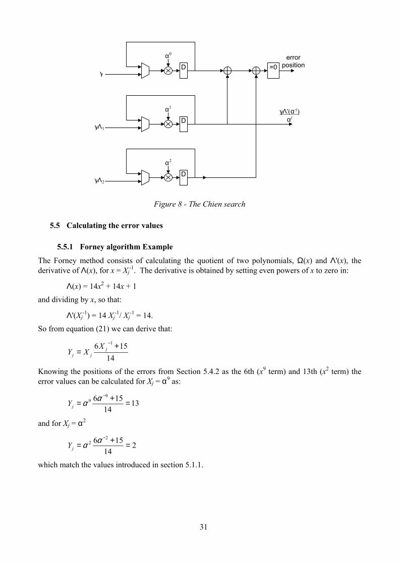
5.5.1 Forney algorithm Example
The Forney method consists of calculating the quotient of two polynomials, Ω(x) and Λ'(x), the derivative of Λ(x), for x = Xj
-1. The derivative is obtained by setting even powers of x to zero in:
Λ(x) = 14x2 + 14x + 1
and dividing by x, so that:
Λ'(Xj-1) = 14 Xj
-1/ Xj-1 = 14.
So from equation (21) we can derive that:
14156 1 +
=−
jjj
XXY
Knowing the positions of the errors from Section 5.4.2 as the 6th (x9 term) and 13th (x2 term) the error values can be calculated for Xj = α9 as:
1314
156 99 =+=
−ααjY
and for Xj = α2
214
156 22 =+=
−ααjY
which match the values introduced in section 5.1.1.

32
5.5.2 Error value hardware
Hardware calculation of the two polynomials, Ω(x) and Λ'(x), can be performed in a similar manner to that for the Chien search shown in Figure 8, in particular, the function value is calculated for each symbol position in the code word in successive clock periods.
Dα0
errorvalue
γΩ0
Dα1
γΩ1
γΛ'(α-j)αj inv
errorposition
Figure 9 - Calculating error values
Thus in Figure 9, there are two circuits producing the values of the Ω1 and Ω0 terms, which are added together. However, the arrangement includes some simplifications, so that the derivative term is obtained directly from the Chien search circuit in Figure 8. It turns out that when code generator polynomial roots beginning with α0 are chosen (b=0), the sum of the odd terms of Λ(x) can be used directly. This provides Λ'(α-j)/αj directly, which eliminates the need to multiply Ω(α-j) by αj. Thus the error value can be obtained by division of the two terms, shown in Figure 9 as inversion and multiplication.
A further point is that the hardware arrangement operates without dividing through by the constant γ as shown at the end of Section 5.3.1. This step is not needed because the multiplying factor cancels in the division so that the error value results are not affected.
5.6 Error correction Errors are corrected by adding the error values Y, to the received symbols R at the positions located by the X values.
5.6.1 Correction example The error values and positions can be formed into an error vector and added to the received code word to produce the corrected message:
x14 x13 x12 x11 x10 x9 x8 x7 x6 x5 x4 x3 x2 x1 x0 0 0 0 0 0 13 0 0 0 0 0 0 2 0 0 1 2 3 4 5 11 7 8 9 10 11 3 1 12 12 1 2 3 4 5 6 7 8 9 10 11 3 3 12 12

33
5.6.2 Correction hardware The AND gate of Figure 9 is enabled at the error positions identified by the Chien search circuit of Figure 8 so that the valid error values are added modulo-2 to the appropriately delayed symbol values of the code word, as shown in Figure 4.
5.7 Implementation complexity Having come this far, the reader will appreciate that the error correction capacity, t, has a strong influence on the complexity of the equations. Also, the number of bits in a symbol, m, affects the complexity of the Galois field arithmetic. Because of the full multiplications involved, the calculations to find the coefficients of the error location polynomial Λ(x) and the error magnitude polynomial Ω(x) form the most complicated part of the decoding process.
It is difficult to provide meaningful gate-count figures for hardware implementations of the coder and decoder because these will depend strongly on the degree of parallelism that is used in the circuitry. It is also possible to exchange complexity for delay in the decoding process. If the logic family is able to support clock rates at a large multiple of the symbol rate (such as 8 times), then the complexity of many parts of the circuit are capable of being reduced by that factor. Also, some designers may feel that a processor-based implementation is appropriate.
For the DVB-T system, the Reed-Solomon coder represents only a small part (say 2-3%) of the whole modulator. The decoder is much more significant, amounting to perhaps about 7% of the demodulator. Considering that the demodulator may be approaching three times the complexity of the modulator, the Reed-Solomon decoder is probably up to ten times the complexity of the coder. To give a different perspective, the Reed-Solomon decoder may be about one quarter of the complexity of the Fast Fourier Transform required for DVB-T.
So far, no mention has been made of erasure processing, in which the locations of the errors are known (through some separate indication from the receiver) but the error values are not. This doubles the error correction capacity of the code and consequently doubles the number of equations to be solved. It therefore represents a substantial increase in complexity over the basic correction process.
6 Conclusion This note has described the theory and methods of Reed-Solomon coding and decoding with a view to facilitating implementation in dedicated hardware. This has particular relevance in implementations of the DVB-T standard.
Reed-Solomon coding circuits for DVB-T have already been implemented in hardware as part of the Digital Radio Camera project. For the decoder, the techniques described have been tested in software for the DVB-T standard and in hardware for simpler codes. It is believed that this has identified many of the pitfalls involved in these processes.
7 References [1] Reed, I. S. and Solomon, G., 1960. Polynomial Codes over Certain Finite Fields, J. SIAM.,
Vol. 8, pp. 300-304, 1960.
[2] ETSI, 1997. Digital broadcasting systems for television, sound and data services; Framing structure, channel coding and modulation for digital terrestrial television. European Telecommunication Standard ETS 300 744.
[3] Bose, R. C. and Chaudhuri, D. K. R., 1960. On a class of error-correcting binary group codes. Inf. Control, Vol. 3, 1960.

34
[4] Hocquenghem, A., 1959. Codes correcteurs d'erreurs, Chiffres., Vol. 2, 1959.
[5] Berlekamp, E. R. Algebraic Coding Theory. McGraw-Hill, New York, 1968.
[6] Purser, M., 1995. Introduction to error-correcting codes. Artech House, Boston, London, 1995.
[7] Pretzel, O. 1992. Error-correcting codes and finite fields. Clarendon Press, Oxford, 1992.
[8] Chien, R. T. 1964. Cyclic decoding procedures for Bose-Chaudhuri-Hocquenghem codes. IEEE Transactions on Information Theory, Vol. IT-10, pp 357- 363.
8 Appendix
8.1 Berlekamp's algorithm
8.1.1 The algorithm Berlekamp's algorithm [6] consists of a series of steps based on improving an approximation to the error locator polynomial Λ(x) using a correction polynomial C(x) and the syndrome values S0 .... S2t-1 as inputs. It also requires a step parameter K and a parameter L which tracks the order of the equations.
Initially we set:
K = 1, L = 0, Λ(x) = 1 and C(x) = x.
Then each step consists of first calculating an error value e using:
∑=
−−Λ+=L
iiKiSSe
110
So initially e = S0.
Then, provided that e is non-zero, we produce Λ*(x), a new approximation to the error locator polynomial, given by:
Λ*(x) = Λ(x) + e × C(x).
If 2L < K, we set L = K - L and form a new correction polynomial from:
C(x) = Λ(x) ÷ e.
If e is zero, these calculations are omitted.
Then we produce a new C(x) by multiplying the old correction polynomial by x, replace Λ(x) by Λ*(x) and increment K. The next step starts with the new values of K, L, Λ(x) and C(x) until K > 2t in which case Λ(x) is the required error locator polynomial.

35
8.1.2 Worked example The syndrome values calculated in Section 5.2.1 are:
S0 = 15, S1 = 3, S2 = 4 and S3 = 12
Step 1:
K L C2 C1 C0 Λ2 Λ1 Λ0 1 0 0 1 0 0 0 1
e = S0 = 15
15 × 0 1 0 → 0 15 0 0 15 1 2L < K, so we set L = K - L = 1 and divide C(x) by e:
1/e = 1/15 = 8
C2 C1 C0 8 × Λ(x) → 0 0 8
Multiply C(x) × x → 0 8 0
Increment K → 2 ≤ 2t = 4, so continue.
Step 2:
K L C2 C1 C0 Λ2 Λ1 Λ0 2 1 0 8 0 0 15 1
e = S1 + Λ1×S0 = 3+15×15 = 9
9 × 0 8 0 → 0 4 0 0 11 1 2L = K, so we skip some steps, then: C2 C1 C0 x × C(x) → 8 0 0
Increment K → 3 ≤ 2t = 4, so continue.
Step 3:
K L C2 C1 C0 Λ2 Λ1 Λ0 3 1 8 0 0 0 11 1
e = S2 + Λ1×S1 = 4+11×3 = 10
10 × 8 0 0 → 15 0 0 15 11 1 2L < K, so we set L = K - L = 2 and divide C(x) by e:
1/e = 1/10 = 12
C2 C1 C0 12 × Λ(x) → 0 13 12
x × C(x) → 13 12 0
Increment K → 4 ≤ 2t = 4, so continue.

36
Step 4:
K L C2 C1 C0 Λ2 Λ1 Λ0 4 2 13 12 0 15 11 1
e = S3 + Λ1×S2 + Λ2×S1 = 12+11×4+15×3 = 4
4 × 13 12 0 → 1 5 0 14 14 1 2L = K, so we skip some steps, then: C2 C1 C0 x × C(x) → 12 0 0
Increment K → 5 > 2t = 4, so the process is complete and Λ(x) = 14x2 + 14x + 1 as before.
8.2 Special cases in the Euclidean algorithm arithmetic There are particular combinations of error values which cause the Euclidean algorithm calculations to depart from the steps shown in Section 5.3.1 and so require the processor of Figure 6 to follow a different sequence. This is necessary when leading zero values occur in the divisor.
8.2.1 Single errors Instead of the two errors introduced in Section 5.1.1, we will introduce only one, so that:
E(x) = E9x9
and we make E9 = 13 as before. Then the syndrome values obtained are:
S0 = 13, S1 = 11, S2 = 2 and S3 = 7
so the syndrome polynomial is:
S(x) = S3x3 + S2x2 + S1x + S0
= 7x3 + 2x2 + 11x + 13
As before, the first step of the algorithm is to divide x2t by S(x), but this time we multiply S(x) × 6x (6 = 1/7) and subtract, followed by multiplying S(x) × 14 (14 = 12/7) and subtracting. This gives the remainder 10. In the right hand process, the initial value 1 is multiplied by the same values used in the division process and added to an initial sum value of zero. So the right-hand calculation produces 0 + 1 × (6x + 14) = 6x + 14.
x4 x3 x2 x1 x0 x2 x1 x0 dividend: 1 0 0 0 0 0 0 divisor × 6x: 1 12 15 8 6 0 12 15 8 0 6 0 divisor × 14: 12 15 8 10 0 14 remainder: 0 0 10 6 14
In this case, the degree of the remainder (=0) is already less than t (= 2) so that the required values are:
γΛ(x) = 6x + 14
and
γΩ(x) = 10.

37
When these values are used in the subsequent processes, the location and value of the error are identified correctly. So for Xj = α9 we find:
γΛ(α-9) = 6(α-9) + 14
= 6(α6) + 14
= 0
and the error value is calculated as:
136
109 ==αjY
8.2.2 Errors that make S3 zero If we change one of the original error values, so that:
E(x) = E9x9 + E2x2
but we make E9 = 7, instead of 13, while E2 = 2, as before. Then the syndrome values obtained are:
S0 = 5, S1 = 11, S2 = 11 and S3 = 0
and the syndrome polynomial is:
S(x) = S3x3 + S2x2 + S1x + S0
= 11x2 + 11x + 5
This time we have to multiply S(x) × 5x2 (5 = 1/11) and subtract, followed by S(x) × 5x (5 = 1/11) and subtracting, and then multiply S(x) × 15 (15 = 3/11) and subtract. This gives the remainder x + 6. In the right hand process, the initial value 1 is multiplied by the same values used in the division process and added to an initial sum value of zero. So the right-hand calculation produces 0 + 1 × (5x2 + 5x + 15) = 5x2 + 5x + 15.
x4 x3 x2 x1 x0 x2 x1 x0 dividend: 1 0 0 0 0 0 0 0 divisor × 5x2: 1 1 2 5 0 0 1 2 0 5 0 0 divisor × 5x: 1 1 2 0 5 0 3 2 0 5 5 0 divisor × 15: 3 3 6 0 0 15 remainder: 1 6 5 5 15
In this case, after a three step division, the degree of the remainder (=1) is already less than t (= 2) so that the required values are:
γΛ(x) = 5x2 + 5x + 15
and γΩ(x) = x + 6.
Again these values lead to the correct locations and values of the errors. So for Xj = α9 we find:
γΛ(α-9) = 5(α-9)2 + 5(α-9) + 15
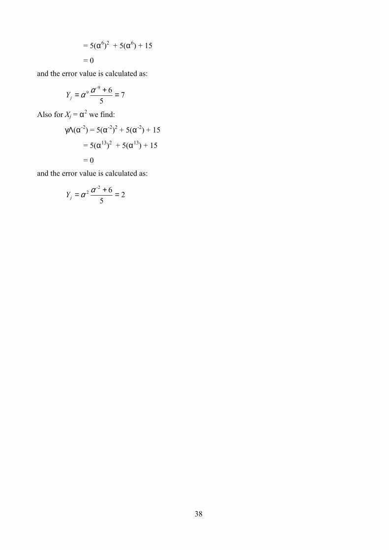
38
= 5(α6)2 + 5(α6) + 15
= 0
and the error value is calculated as:
75
6 -99 =+= ααjY
Also for Xj = α2 we find:
γΛ(α-2) = 5(α-2)2 + 5(α-2) + 15
= 5(α13)2 + 5(α13) + 15
= 0
and the error value is calculated as:
25
6 -22 =+= ααjY

39
8.3 Arithmetic look-up tables for the examples Tables 7 and 8 below show the results for addition of two field elements (Table 7) and multiplication of two field elements (Table 8) in the sixteen element Galois field with the field generator polynomial 1)( 4 ++= xxxp .
0 1 2 3 4 5 6 7 8 9 10 11 12 13 14 15 0 0 1 2 3 4 5 6 7 8 9 10 11 12 13 14 15 1 1 0 3 2 5 4 7 6 9 8 11 10 13 12 15 14 2 2 3 0 1 6 7 4 5 10 11 8 9 14 15 12 13 3 3 2 1 0 7 6 5 4 11 10 9 8 15 14 13 12 4 4 5 6 7 0 1 2 3 12 13 14 15 8 9 10 11 5 5 4 7 6 1 0 3 2 13 12 15 14 9 8 11 10 6 6 7 4 5 2 3 0 1 14 15 12 13 10 11 8 9 7 7 6 5 4 3 2 1 0 15 14 13 12 11 10 9 8 8 8 9 10 11 12 13 14 15 0 1 2 3 4 5 6 7 9 9 8 11 10 13 12 15 14 1 0 3 2 5 4 7 6 10 10 11 8 9 14 15 12 13 2 3 0 1 6 7 4 5 11 11 10 9 8 15 14 13 12 3 2 1 0 7 6 5 4 12 12 13 14 15 8 9 10 11 4 5 6 7 0 1 2 3 13 13 12 15 14 9 8 11 10 5 4 7 6 1 0 3 2 14 14 15 12 13 10 11 8 9 6 7 4 5 2 3 0 1 15 15 14 13 12 11 10 9 8 7 6 5 4 3 2 1 0
Table 7 - Addition table for use in the worked examples
0 1 2 3 4 5 6 7 8 9 10 11 12 13 14 15 0 0 0 0 0 0 0 0 0 0 0 0 0 0 0 0 0 1 0 1 2 3 4 5 6 7 8 9 10 11 12 13 14 15 2 0 2 4 6 8 10 12 14 3 1 7 5 11 9 15 13 3 0 3 6 5 12 15 10 9 11 8 13 14 7 4 1 2 4 0 4 8 12 3 7 11 15 6 2 14 10 5 1 13 9 5 0 5 10 15 7 2 13 8 14 11 4 1 9 12 3 6 6 0 6 12 10 11 13 7 1 5 3 9 15 14 8 2 4 7 0 7 14 9 15 8 1 6 13 10 3 4 2 5 12 11 8 0 8 3 11 6 14 5 13 12 4 15 7 10 2 9 1 9 0 9 1 8 2 11 3 10 4 13 5 12 6 15 7 14 10 0 10 7 13 14 4 9 3 15 5 8 2 1 11 6 12 11 0 11 5 14 10 1 15 4 7 12 2 9 13 6 8 3 12 0 12 11 7 5 9 14 2 10 6 1 13 15 3 4 8 13 0 13 9 4 1 12 8 5 2 15 11 6 3 14 10 7 14 0 14 15 1 13 3 2 12 9 7 6 8 4 10 11 5 15 0 15 13 2 9 6 4 11 1 14 12 3 8 7 5 10
Table 8 - Multiplication table for use in the worked examples


