61
RDBMS vs NoSQL: Performance and Scaling Comparison Christoforos Hadjigeorgiou August 23, 2013 MSc in High Performance Computing The University of Edinburgh Year of Presentation: 2013
RDBMS vs NoSQL: Performance and ScalingComparison
Christoforos Hadjigeorgiou
August 23, 2013
MSc in High Performance Computing
The University of Edinburgh
Year of Presentation: 2013

Abstract
The massive amounts of data collected today by software in fields varying from academiato business and many other fields, is increasingly becoming a huge problem due to stor-age technologies not advancing fast enough to provide the performance scalability needed.This is even more true for data which are highly organised and require analysis while beingstored in databases and being accessed by various applications simultaneously. Databasesalso have the added advantage of providing failover mechanism in case of disruptions orone node failing.
As database vendors struggle to gain more market share new technologies emerge at-tempting to overcome the disadvantages of previous designs while providing more features.Two popular database types, the Relational Database Management Systems and NoSQLdatabases are examined. The aim of this project was to examine and compare two databasesfrom these two database models and answer the question of whether one performs and scalesbetter than the other.
From the comparison of the results it was found that MongoDB can perform muchbetter for complicated queries at the cost of data duplication which in turn results to alarger database. Also the database size did not appear to be a deciding factor as performancewas not crippled significantly for larger database sizes. Writing benchmarks were also runwhich showed that MySQL performs best at deletion whereas MongoDB excels at insertingdocuments. The last comparison showed that using sharding to split up the database inMongoDB did not provide a performance advantage which may be related to the routingdone by the MongoDB system.
Contents
1 Introduction 1
2 Background 32.1 Databases . . . . . . . . . . . . . . . . . . . . . . . . . . . . . . . . . . 32.2 Relational Databases . . . . . . . . . . . . . . . . . . . . . . . . . . . . . 32.3 ACID properties . . . . . . . . . . . . . . . . . . . . . . . . . . . . . . . 42.4 NoSQL Databases . . . . . . . . . . . . . . . . . . . . . . . . . . . . . . 52.5 Other databases . . . . . . . . . . . . . . . . . . . . . . . . . . . . . . . 5
2.5.1 Navigational Databases . . . . . . . . . . . . . . . . . . . . . . . 62.5.2 Object-oriented databases . . . . . . . . . . . . . . . . . . . . . . 6
2.6 Database Replication . . . . . . . . . . . . . . . . . . . . . . . . . . . . . 62.7 Database Sharding . . . . . . . . . . . . . . . . . . . . . . . . . . . . . . 82.8 EPCC Data Intensive Machine 1 (EDIM1) . . . . . . . . . . . . . . . . . 8
2.8.1 ROCKS Linux . . . . . . . . . . . . . . . . . . . . . . . . . . . . 92.8.2 GNU Parallel . . . . . . . . . . . . . . . . . . . . . . . . . . . . . 9
3 Benchmarks 103.1 Benchmarking harness . . . . . . . . . . . . . . . . . . . . . . . . . . . . 103.2 Measurements . . . . . . . . . . . . . . . . . . . . . . . . . . . . . . . . 113.3 Measurement metrics . . . . . . . . . . . . . . . . . . . . . . . . . . . . 113.4 Database schema . . . . . . . . . . . . . . . . . . . . . . . . . . . . . . 123.5 Database Queries . . . . . . . . . . . . . . . . . . . . . . . . . . . . . . 153.6 Benchmarking configurations . . . . . . . . . . . . . . . . . . . . . . . . 163.7 Database configurations . . . . . . . . . . . . . . . . . . . . . . . . . . . 16
3.7.1 Single node . . . . . . . . . . . . . . . . . . . . . . . . . . . . . . 163.7.2 Multiple Nodes . . . . . . . . . . . . . . . . . . . . . . . . . . . . 173.7.3 Sharding . . . . . . . . . . . . . . . . . . . . . . . . . . . . . . . 17
4 Results and Analysis 204.1 Query types . . . . . . . . . . . . . . . . . . . . . . . . . . . . . . . . . 204.2 MongoDB Sharding . . . . . . . . . . . . . . . . . . . . . . . . . . . . . 304.3 Database size . . . . . . . . . . . . . . . . . . . . . . . . . . . . . . . . 32
i

CONTENTS ii
5 Conclusion 355.1 Deviations from the project plan . . . . . . . . . . . . . . . . . . . . . . . 365.2 Future work . . . . . . . . . . . . . . . . . . . . . . . . . . . . . . . . . 37
A Benchmark Results 39A.1 MongoDB . . . . . . . . . . . . . . . . . . . . . . . . . . . . . . . . . . 39A.2 MySQL . . . . . . . . . . . . . . . . . . . . . . . . . . . . . . . . . . . . 39
B Configuration and Scripts 50B.1 MongoDB . . . . . . . . . . . . . . . . . . . . . . . . . . . . . . . . . . 50B.2 MySQL Cluster . . . . . . . . . . . . . . . . . . . . . . . . . . . . . . . 51B.3 Harness . . . . . . . . . . . . . . . . . . . . . . . . . . . . . . . . . . . . 51
B.3.1 Building . . . . . . . . . . . . . . . . . . . . . . . . . . . . . . . 51B.3.2 RUNNING . . . . . . . . . . . . . . . . . . . . . . . . . . . . . . 52
B.4 Parallel Shell Script . . . . . . . . . . . . . . . . . . . . . . . . . . . . . 52

List of Figures
2.1 Database schema example . . . . . . . . . . . . . . . . . . . . . . . . . . 42.2 MongoDB Replica deployment and usage . . . . . . . . . . . . . . . . . . 7
3.1 Relational database schema . . . . . . . . . . . . . . . . . . . . . . . . . 133.2 MongoDB Schema . . . . . . . . . . . . . . . . . . . . . . . . . . . . . . 143.3 MySQL Cluster Architecture . . . . . . . . . . . . . . . . . . . . . . . . . 17
4.1 Simple query with different configurations . . . . . . . . . . . . . . . . . . 214.2 Simple queries, total number of queries per second . . . . . . . . . . . . . 214.3 Multiple benchmark configurations with simple query measuring queries/sec-
ond with larger number of queries . . . . . . . . . . . . . . . . . . . . . . 224.4 Simple query - Queries per second for total number of threads . . . . . . . 234.5 INNER JOIN query using multiple configurations . . . . . . . . . . . . . . 244.6 INNER JOIN query, queries/second for 500 and 1000 queries . . . . . . . 254.7 INNER JOIN QUERY two runs multiple configurations . . . . . . . . . . . 254.8 Nested SELECT query . . . . . . . . . . . . . . . . . . . . . . . . . . . . 264.9 Nested SELECT query queries/second . . . . . . . . . . . . . . . . . . . . 264.10 Nested SELECT query scatter plot . . . . . . . . . . . . . . . . . . . . . 274.11 2 INNER JOINS & subquery . . . . . . . . . . . . . . . . . . . . . . . . . 284.12 2 INNER JOINS & subquery, queries per second . . . . . . . . . . . . . . 284.13 2 INNER JOINS & subquery, number of threads . . . . . . . . . . . . . . 294.14 INSERT and DELETE operations . . . . . . . . . . . . . . . . . . . . . . 304.15 MongoDB Replica and Shard configurations, simple query . . . . . . . . . 314.16 MongoDB Replica and Shard configurations, complex query . . . . . . . . 314.17 MongoDB Shard and MySQL, complex query . . . . . . . . . . . . . . . . 324.18 Simple query with different database sizes . . . . . . . . . . . . . . . . . . 334.19 Complex query with different database sizes . . . . . . . . . . . . . . . . . 34
iii

Acknowledgements
I would like to sincerely thank Dr Adam Carter. Without his advice, guidance and encour-agement this dissertation would not have been possible.
I am also very grateful to Mr Gareth Francis for helping in setting up the cluster andtroubleshooting.
I would like to thank my family as without their support this Master’s degree would nothave been possible for me.

Chapter 1
Introduction
Efficient storage and retrieval of data has always been an issue due to the growing needsin industry, business and academia. Larger amounts of transactions and experimentationresult in massive amounts of data which require organised storage solutions. Databaseswere created in order to satisfy this need of storing and retrieving data in an organisedmanner. Since their inception in the 1960’s different types have emerged, each using itsown representation of data and technology for handling transactions. They began withnavigational databasess which were based on linked-lists, moved on to relational databases,afterwards object-oriented and in the late 2000s NoSQL emerged and has become a populartrend [1].
Two of the most widely used database types are relational databases and NoSQLdatabases. Although NoSQL databases are relatively new compared to other types theyhave become popular due to their ability to handle very fast unrelated and unstructureddata, mainly because they do not require a fixed schema and they use metadata heavilyin order to achieve fast performance. Relational databases came to the forefront in themid 1970’s and were proven successful by the end of the decade. The essential conceptsinvolved in relational databases were laid out by Edgar Codd in order to overcome thedisadvantages of the previous linked lists implementations in databases.
Although the two types differ in many aspects depending on the implementation theycould be used for similar applications although it is not recommended as one is not meantas an alternative to the other [2]. One of the main reasons for this recommendation is theproblem of NoSQL databases being less reliable compared to relational databases due toless data-integrity and reliability. Through this dissertation a comparison of the two typesis performed in terms of performance and scalability. Scalability in databases is their abilityto handle an increasing amount of transactions and stored data at the same amount oftime. The NoSQL database MongoDB and the relational database MySQL Cluster, whichwill be the databases tested, support separating the data stored to different nodes andhave support for a number of programming languages. Other databases were consideredas well but due to previous experience with MySQL and the simple programming layout
1
CHAPTER 1. INTRODUCTION 2
of MongoDB as well as its document structure these two were preferred. The databasesconsidered were PostgreSQL, CouchDB and Apache Cassandra. The reasons why thesedatabases were not chosen include tuning of the configuration in order to achieve goodperformance for PostgreSQL and the limitation of interface to HTTP/REST API and Javafor CouchDB and Apache Cassandra respectively. [3] [4] [5]
Comparing these two databases is important as it allows to draw conclusions regardingtheir ability to process data and how they handle large amounts of transactions and data.It also provides insight to how well suited they are to today’s issue of massive amounts ofdata collected otherwise known as Big Data. Databases play an important role in applica-tions and the wrong choice at the beginning may have disastrous effects as it is difficult tomigrate to another database system, more so a completely different type. The performanceand scalability of the databases are the most important factors besides reliability whenweighing the various options and comparing them for different databases can be difficultdue to different designs, configurations and data access methods.
This dissertation takes the two database systems and compares them by trying to finda middle ground where their implementations are as close as possible and the benchmarksperformed do not favour one database system over the other. Amongst the most importantissues are finding a data set and representing it in both databases effectively. In additionthe correct choice of benchmarks is vital as stressing a database can be a tedious task.
Chapter 2 is an analysis of the technologies used followed by an analysis of relationaland NoSQL databases. Also the terminology and concepts used in developing databases isdiscussed. An overview of the machine used in the experiments, EDIM1, is provided at theend of the chapter together with a description of the operating system and the softwareused to run the benchmark in parallel.
Chapter 3 details the design of the software used for the experiments. This includes anexamination of the database deployed for each database system. The methodology usedfor measuring the performance and scalability of the databases is described together withwhat options were available in doing so.
Chapter 4 analyses the results of the experiments and builds a hypothesis regarding theperformance of the databases. This hypothesis is then examined through further experi-mentation.

Chapter 2
Background
2.1 DatabasesDatabases are defined as organised collections of data [6, p. 6]. Although when usingthe term database we refer to the entire database system, the term actually refers only tothe collection and the data. The system which handles the data, transactions, problemsor any other aspect of the database is the Database Management System (DBMS). Whatfollows is a description of the two database types which will be compared in this dissertation.
Early designs and implementations were based on the use of linked lists to create re-lations between data and to find specific data. These models were not standardised andrequired extensive training in order to make efficient use of them. These models and otherimportant types are explained briefly as well.
2.2 Relational DatabasesRelational databases use the notion of databases separated into tables where each columnrepresents a field and each row represents a record. Tables can be related or linked witheach other with the use of foreign keys or common columns. On an abstract level tablesrepresent entities, such as users, customers or suppliers. This abstraction is helpful whendesigning the database schema as real world objects need to be mapped to the databasein addition with the relations between them. The design of a database schema can bevisualised using diagrams such as the one in Figure 2.1.
3

CHAPTER 2. BACKGROUND 4
Figure 2.1: Database schema example
An important design aspect of relational databases is the normalisation of the schema.This involves 3 steps which are described below:
1. First Normal Form (1NF): Eliminate groups of repeating data by creating a newtable for each group of related data which is identified by a primary key.
2. Second Normal Form (2NF): If a set of values are the same for multiple recordsmove them to a new table and link the two tables with a foreign key.
3. Third Normal Form (3NF): Fields which do not depend on the primary key of atable must be removed and if necessary be put into another table.
It is also necessary for a database schema to satisfy the 2NF to first satisfy 1NF and thesame applies for 3NF correspondingly. While there are other forms a schema is considerednormalised if it satisfies the above 3 conditions.
2.3 ACID propertiesAn important aspect of relational databases which guarantees the reliability of transactionsis their adherence to the ACID properties: Atomicity, Consistency, Isolation, Durability [6,p. 405]. Each property is explained below in the context of databases.
• Atomicity: Either all parts of a transaction must be completed or none.
• Consistency: The integrity of the database is preserved by all transactions. Thedatabase is not left in an invalid state after a transaction.
• Isolation: A transaction must be run isolated in order to guarantee that any incon-sistency in the data involved does not affect other transactions.
• Durability: The changes made by a completed transaction must be preserved or inother words be durable.
CHAPTER 2. BACKGROUND 5
2.4 NoSQL DatabasesNoSQL databases started gaining popularity in the 2000’s when companies began investingand researching more into distributed databases [7]. For this reason the category of NoSQLdatabases grew and included many subtypes each better suited to specific datasets thanothers. The most common NoSQL database categories are the following:
• Document stores: The notion of "documents" is the central concept here withdocuments being the equivalent of records in relational databases and collectionsbeing similar to tables. [8]
• Key-value stores: Data is stored as values with a key assigned to each value similarlyto hash-tables. Also depending on the database a key can have a collection ofvalues. [8]
• Graph databases: Like graph theory the notion of nodes and edges is the primaryconcept in graph databases. Nodes correspond to entities such as a user or a musicrecord and edges represent the relations between the nodes. An important aspectwhich differentiates graph from relational databases is the use of index-free adjacency,this means each element contains a pointer to its adjacent element and does notrequire indexing of every element. [9]
An important aspect of NoSQL databases is that they have no predefined schema,records can have different fields as necessary, this may be referred to as a dynamic schema.Many NoSQL databases also support replication which is the option of having replicas ofa server, this provides reliability as in the case one goes offline the replica would becomethe primary server. All servers execute the same transactions and synchronise their datain order to eliminate any errors. Also an important difference between relational databasesand NoSQL databases is they do not fully guarantee ACID properties. Their lack of ACIDguarantees is attributed to their deployment architeture which typically involves havingmultiple nodes in order to achieve horizontal scalability and recovery in case of failover.This deployment, which is also referred to as replication, creates issues with synchronisationwhich can result in a secondary node becoming primary but not have an up-to-date copy ofthe data. NoSQL databases, apart from using an Application Programming Interface(API)or query language to access and modify data, may also use the MapReduce method which isused for performing a specific function on an entire dataset and retrieving only the result. [2]
2.5 Other databasesBeyond relational and NoSQL databases other types have emerged in the past as well.Thesetypes have not become as successful as the types examined in this project but have beenan important part of the evolution of databases nonetheless.

CHAPTER 2. BACKGROUND 6
2.5.1 Navigational DatabasesNavigational Databases were the first generation of databases developed which worked byusing pointers from one record to another. The major downside of navigational databaseswas the fact that the user would have to know and understand the underlying physicalstructure of the database in order to query for records. In order for an extra field to beadded to a database the entire underlying storage scheme had to be rebuilt. In addition thelack of standardisation among vendors was a disadvantage as it became difficult to choosea suitable implementation. [1]
2.5.2 Object-oriented databasesAn important part of the database evolution are object-oriented databases which emergedin the 1980s and their main usage was in the object-oriented field such as in conjunc-tion with object-oriented programming languages. In this model information was storedas objects which could accommodate for a large number of data types and could alsooffer advanced features such as inheritance and polymorphism which were characteristicof object-oriented programming languages as well. The disadvantages which preventedobject-oriented databases from gaining more popularity was the need to rebuild an entiredatabase in order to migrate from another database management system and also the issuethat most of these databases were bound to a specific programming language. [1]
Object Relational Database Management System & Object Relational Mapping
In order to overcome the disadvantages of object-oriented database and use the advantagesof relational databases the Object Relational Database Management System emerged. Thissystem attempted to bring together the features of RDBMSs and object-oriented modellingtechniques which were used in popular programming languages. This however was notsuccessful with a more popular approach being the Object Relational Model whereby arelational model database was used with an object relational mapping software which alloweddevelopers to integrate their own types and their methods into the DBMS. [1]
2.6 Database ReplicationDatabase Replication is the practice of deploying multiple servers which are clones of eachother. This practice is used in NoSQL databases often in order to provide higher reliabilityand performance. MongoDB recommends deploying a replica set, which is a set of replicaservers, in all production deployments. [10]
In MongoDB replication is deployed using a primary-secondary server configurationwhereby one server is the primary and all others are secondary. The primary server, orprimary replica, handles all write operations and logs them in a special collection where thesecondaries read and apply them. Secondary replica servers can also read the operations

CHAPTER 2. BACKGROUND 7
from another secondary thus limiting the amount of load on the primary server. This pro-cesses are shown in Figure 2.2. By having a copy of the data replica servers not only providemore reliability but can also be used for read operations from client applications, this canhave a massive performance effect but also carries with it the chance that the data providedwill not be the most up-to-date. The reason that data is not always up to date is due tothe asynchronous replication model which MongoDB uses. This asynchronous replicationsprovides better reliability as secondary members can continue to function when anothermember of the replica set is unavailable but prohibits the guarantee of the ACID propertiesas a secondary replica which becomes primary may not be up to date thus violating theConsistency and Durability properties.
Figure 2.2: MongoDB Replica deployment and usage
In the case when the primary replica fails for any reason and goes offline voting takesplace to promote a secondary replica to primary, this is when the concept of an arbiterserver becomes relevant. An arbiter server does not handle any load or store data but onlyexists to provide a vote in these elections, this is necessary in cases where there is an evennumber of secondary replicas and the voting could result in a draw.
MySQL Cluster also supports replication but is currently limited to a main replica serverand a slave replica server at maximum. This limitation can be alleviated with the useof node clusters which work as replicas of other node clusters. In addition, the defaultconfiguration does not allow direct connections to the replica in order to distribute theload and also the use of replication in clustering instead of thte simple Master-Slave modelrequires the use of the NDB engine to cluster successfuly. The MySQL implementation ofthe Master-Slave model is similar to MongoDB as it is used to send write operations to the

CHAPTER 2. BACKGROUND 8
Master node and read queries can be routed accordingly either to the Master or the Slave.This enables to distribute some of the load from the Master node and improve performance.
2.7 Database ShardingSharding is the term used to describe practice of using multiple servers of the same databaseand configuring them in order for the data stored in the database to be split or separatedto different machines. This allows increased performance as each server handles differentsets of data thus if a single database becomes too large its performance may diminish dueto the increased time a query takes. Despite the obvious advantage of added performancedatabase, replication is recommended over sharding as it provides both performance andreliability. Specifically MongoDB developers suggest to deploy databases without shardingand only shard when the data set increases in size. In addition, MongoDB shards can beaccessed directly but the transactions which can be performed are limited to the collectionswhich are sharded on the specific shard.
MySQL Cluster handles sharding automatically but is limited to using the NDB storageengine. The NDB storage engine is limited mainly due to its lack of foreign keys supportand a storage limit of 3TB compared to 64TB of the InnoDB storage engine [11] makingit unsuitable for the benchmarking harness which uses foreign keys.
2.8 EPCC Data Intensive Machine 1 (EDIM1)EDIM1 is an experimental platform designed for data-intensive research at EPCC. It consistsof 120 back-end nodes, a login node and data staging server. Each back-end node consistsof an Intel Atom CPU, a programmable GPU, 4GB of memory, a 6TB hard disk and 256GBSSD. Nodes are also interconnected with a gigabit ethernet network and use ROCKS asthe operating system which is a GNU/Linux distribution designed for running clusters [12].EDIM1 was designed as an Amdahl-balanced cluster in order to eliminate the I/O bottleneckwhich exists in most systems due to the inability of the I/O system to provide data as fastas the CPU can process it. This is an important feature of the machine which affects theproject as the databases will be able to make use of all the processing power instead ofdelaying while the I/O is sending data. The significance of this effect is that observationscan be made on how the database works according to the number of connections it handles.For example, having two simultaneous connections requesting the same data could cause aslow down to the transations.

CHAPTER 2. BACKGROUND 9
2.8.1 ROCKS LinuxThe operating system running on EDIM1 is the ROCKS Linux is a GNU/Linux distributionwhich is aimed at setting up clusters easily. It is a 64 bit operating system which allowsto build, manage and monitor clusters through a frontend which controls the rest of thenodes. In case of a node failing the frontend automatically reinstalls the base system onthat node any preselected packages which in ROCKS are called rolls. [13]
2.8.2 GNU ParallelAs the default installation of ROCKS Linux on EDIM1 lacked a parallel programming libraryand using one was beyond the aim of the project an alternative method was used. Thesoftware package of the open source GNU Parallel program was installed which allows toexecute commands and scripts in parallel by specifying the number of threads. This wasused in conjunction with the rocks command which is part of the operating system toexecute the benchmarking package multiple times on multiple nodes. [14]

Chapter 3
Benchmarks
3.1 Benchmarking harnessThe benchmarking harness was built using the C programming language and used the lateststable drivers available for each database. Database drivers are the libraries which providea method for connecting with the database and performing transactions.
The harness allows to change different options such as the number of benchmarks andqueries to be performed, the use of random strings for populating the database and whetherto populate the database or use the data already there. Specifically the procedure followedby the harness is as follows:
1. Depending on the database selected create a connection using either the defaultvalues or user-supplied parameters.
2. If database populating was requested the current tables are dropped and repopulatedeither with random strings or a string differentiated by adding an index integer.
3. Otherwise if no populating was requested the database is queried and the data isstored to be used during the benchmarking.
4. Each benchmark is performed which include a simple query, a complicated join oper-ation and a similar complicated operation which uses nested queries instead.
5. The time spent for each benchmark is recorded and at the end of all benchmarks anaverage is calculated and all the results are output.
Since all the actions performed are crucial to measuring the performance correctly thebenchmarking harness will halt if at any point an operation fails. This is also important forfinding errors related to the configuration of the database.
10

CHAPTER 3. BENCHMARKS 11
3.2 MeasurementsThree C methods were considered for taking time measurements . The first was to use theclock() function provided by C but was quickly ruled out as it only provides the time aprocess spent using the CPU. Although this could be used in conjunction with other func-tions to estimate the time which was spent for a benchmark other better and more directmethods were investigated. The second method was the gettimeofday() function whichprovided timings with millisecond accuracy. Due to a misconception on how the MySQL Cdriver works, specifically the MySQL database does not return the result of a query until itis requested to do so, it resulted in getting a different time record compared to what wasexpected. This had the consequence of investigating the use of the MPI_Time functionbut it was quickly ruled out as MPI and its libraries were not installed, a process which couldtake a large amount of time relative to the time available for the entire dissertation. Insteadafter investigating the reason for the unexpected results reported by gettimeofday() andthe explanation was found subsequent timings were as expected.
Each database also offers its own method for measuring time. MySQL can recordqueries which take longer than a predefined amount of time to the Slow Query Log ora system database. By default the time threshold for logging a slow query is 10 secondsand can be configured for microsecond accuracy. Despite the convenience of the automaticlogging it holds some disadvantages to using the timing functions of the harness. First, thelog takes times for individual queries complicating the analysis of the overall result. This isdue to the large size of the log file and the more complicated logging format used as eachquery is also recorded in the log together with other information such as number of rowsreturned. MySQL offers a tool for analysing the log file but its purpose is to summarise thecontents, either by sorting the queries or select queries which match a specific pattern, allof which do not assist in measuring the overall performance of the database. Secondly, thelog itself is a method for measuring time from the server itself and not a client application.This is not an ideal measurement as time will also be spent for applications to retrieve theresult. [15]
MongoDB records query times in a similar manner but the results are stored in a systemspecific database and collection, system.profile. This method is inadequate for measuringperformance due mainly to the lack of overall measuring of performance but also as it hasa minor effect on performance [2].
3.3 Measurement metricsTo measure the performance of the databases a common metric is required. The mostimportant factor for an application is the time required for completing a task, and in thecase of databases the time required to complete a transaction. The benchmarking harnessmeasures the time required to complete a set number of transactions as each transaction

CHAPTER 3. BENCHMARKS 12
on its own is negligible. Also the average of all the benchmarks during a single run ofthe benchmarking harness is calculated in order to have a better overall idea of how thedatabase behaves as a single benchmark may deviate due to outside factors such as anoperating system process temporarily using the CPU or performing I/O. Furthermore, tomeasure the performance of the databases and their scalability the metric of total queriesper second is used as it allows to extrapolate how well the databases cope with differentloads and different numbers of connections. To calculate the queries per second the formulain Figure 3.1 is used
Queries per second = Total number of queries ∗ Total number of threads
Average query time(3.1)
Another metric used is the total queries per second per in order to quantify how thedatabases respond to each thread.
Queries per second per thread = Total number of queries
Average query time(3.2)
3.4 Database schemaThe database schema used was designed from the ground up and was modelled around amusic application which would use different algorithms to suggest songs to users accordingto their tastes and other users who have similar tastes. The database schema shown inFigure was designed for the MySQL database implementation. It has been normalised andeliminates any data duplication between tables. The database schema is shown in Figure3.1.

CHAPTER 3. BENCHMARKS 13
Figure 3.1: Relational database schema
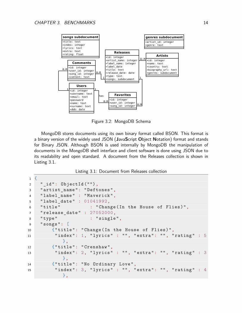
Although the same schema can be informally used in MongoDB some compromiseshave been made to make up for the fact that MongoDB does not support complicatedoperations such as JOINS which are typical for RDBMSs. Instead the MongoDB databaseschema combines a number of tables to take advantage of sub-documents. The processof combining tables is denormalisation although in this case it is only partial, completedenormalisation would mean the combination of all the tables into a single table. In addition,the design of the MongoDB schema allows to more directly compare with MySQL for similartasks such as JOINs or nested SELECTs. In Figure 3.2 the schema for MongoDB is shownincluding the subdocuments which were adapted from the relational schema. The Releasecollection now includes the attributes from the Labels table as each record only has one labeland also includes a songs subdocument which replaces the Songs table. The justificationfor using a subdocument for the songs in each release is that typically the number of songsis relatively small, 10-20, and also they do not change after a release is made. In addition,MongoDB allows faster transactions when dealing with subdocuments compared to findingdata in other collections due to the binary format it uses for internal representation.
CHAPTER 3. BENCHMARKS 14
Figure 3.2: MongoDB Schema
MongoDB stores documents using its own binary format called BSON. This format isa binary version of the widely used JSON (JavaScript Object Notation) format and standsfor Binary JSON. Although BSON is used internally by MongoDB the manipulation ofdocuments in the MongoDB shell interface and client software is done using JSON due toits readability and open standard. A document from the Releases collection is shown inListing 3.1.
Listing 3.1: Document from Releases collection1 {2 "_id": ObjectId (""),3 " artist_name ": " Deftones ",4 " label_name " : " Maverick ",5 " label_date " : 01041992,6 "title" : "Change(In the House of Flies)",7 " release_date " : 27052000,8 "type" : "single",9 "songs": [
10 {"title": "Change(In the House of Flies)",11 "index": 1, "lyrics" : "", "extra": "", "rating" : 5
},12 {"title": " Crenshaw ",13 "index": 2, "lyrics" : "", "extra": "", "rating" : 3
},14 {"title": "No Ordinary Love",15 "index": 3, "lyrics" : "", "extra": "", "rating" : 4
},

CHAPTER 3. BENCHMARKS 15
16 ]17 }
3.5 Database QueriesThe benchmarks involved using three queries to stress the databases. The first query whichwas a simple query containing only a SELECT statement, a second more complex one withan INNER JOIN and a third with a SELECT statement containing an INNER JOIN to asecond table and inside the WHERE clause a nested SELECT containing an INNER JOINas well. In addition a second version of the complex query which contained a single INNERJOIN was created using nested SELECTs as to benchmark the performance of MySQL whena query similar the actions performed in MongoDB is used. These queries are described inSQL terms and are shown in Listing 3.2.
Listing 3.2: Database queries// s imp l e
SELECT ∗ FROM Use r s WHERE username = ’ username ’
// complex 1 .1
SELECT ’ F a v o u r i t e s . song_id ’ AS fSID ,’ F a v o u r i t e s . u s e r_ i d ’ AS fUID
FROM Fa v o u r i t e s AS b INNER JOIN Fa v o u r i t e s AS aON b . u s e r_ i d = a . u s e r_ i dWHERE a . song_id = 123456 AND a . u s e r_ i d != 987654
// complex 1 .2SELECT ’ F a v o u r i t e s . song_id ’ AS fSID ,
’ F a v o u r i t e s . u s e r_ i d ’ AS fUIDFROM Fa v o u r i t e sWHERE u s e r_ i d IN
(SELECT ’ F a v o u r i t e s . u s e r_ i d ’ AS f i dFROM Fa v o u r i t e sWHERE song_id = 123456 AND u s e r_ i d != 987654
// complex 2SELECT ’ Songs . r e l e a s e _ i d ’ AS s I d ,
’ R e l e a s e s . i d ’ AS r I dFROM Songs INNER JOIN Re l e a s e sON Songs . r e l e a s e _ i d = Re l e a s e s . i dWHERE a r t i s t _ i d IN

CHAPTER 3. BENCHMARKS 16
(SELECT ’ Genres . a r t i s t _ i d ’ AS gAIDFROM Genres AS cINNER JOIN A r t i s t s AS dON c . a r t i s t _ i d = d . i d WHERE d . name = ’ a r t i s t_name ’
3.6 Benchmarking configurationsThe benchmarking configurations varied from one to four benchmarking harnesses on eachnode in parallel. The reason for limiting the maximum number of harnesses to four on eachnode is due to the CPU having two hyperthreaded cores which virtually appear as four cores,running more harnesses than the number of available cores could affect the performanceand in consequence the results.
Other configurations were used as well to examine the behaviour of the database. Theseconfigurations included running a single harness on two nodes instead of two harnesses onthe same node. To run the harnesses in parallel on a single node the GNU Parallel programwas used and to run harnesses on multiple nodes GNU parallel was used together with therocks command by specifying which nodes and which command to run on each node.
An important aspect of the dissertation is to compare the performance of the databasedepending on the database size. For this benchmark the harness was first run to populatethe database with a specific amount of data and run some initial tests. Then the harness wasrun again but only to perform benchmarks on the existing data and take time measurements.The reason for running a number of initial benchmarks is due to indexing and as MySQLin particular performed badly.
3.7 Database configurationsThe database systems can be configured in various ways to take advantage of features suchas replication and sharding. For this dissertation the configurations for each database werechanged to examine different situations and set-ups.
3.7.1 Single nodeThe simplest configuration for both databases was to use a single data node without anyreplicas or shards. MySQL is slightly more complicated to configure compared to MongoDBwhich only requires a single mongod instance to be executed. For MySQL a managementnode, a data node and a MySQL daemon process are required. The management nodehandles how the cluster is configured in terms of node groups, replicas, shards, shut-down/restart situations and arbitrating when a master fails whereas the daemon processhandles connections and transactions.
CHAPTER 3. BENCHMARKS 17
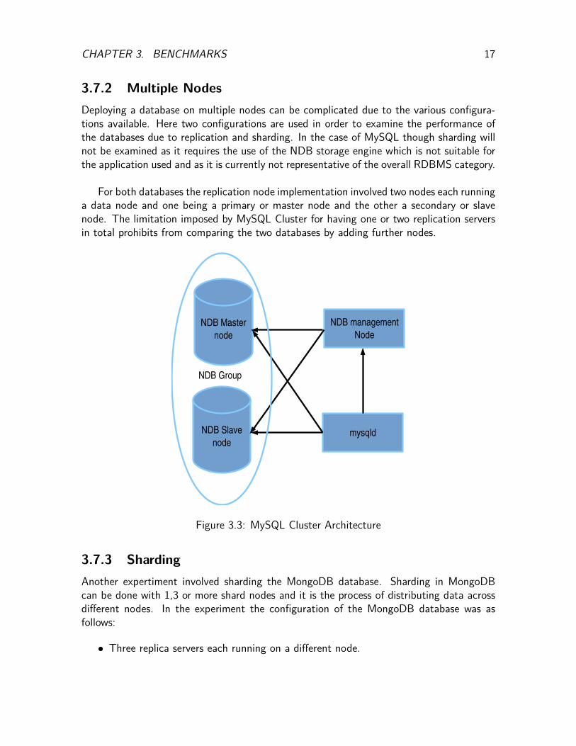
3.7.2 Multiple NodesDeploying a database on multiple nodes can be complicated due to the various configura-tions available. Here two configurations are used in order to examine the performance ofthe databases due to replication and sharding. In the case of MySQL though sharding willnot be examined as it requires the use of the NDB storage engine which is not suitable forthe application used and as it is currently not representative of the overall RDBMS category.
For both databases the replication node implementation involved two nodes each runninga data node and one being a primary or master node and the other a secondary or slavenode. The limitation imposed by MySQL Cluster for having one or two replication serversin total prohibits from comparing the two databases by adding further nodes.
Figure 3.3: MySQL Cluster Architecture
3.7.3 ShardingAnother expertiment involved sharding the MongoDB database. Sharding in MongoDBcan be done with 1,3 or more shard nodes and it is the process of distributing data acrossdifferent nodes. In the experiment the configuration of the MongoDB database was asfollows:
• Three replica servers each running on a different node.

CHAPTER 3. BENCHMARKS 18
• Three configuration servers (mongod –configsvr) each running on the same node asa replica server.
• A query router instance (mongos) which chooses which node will execute a queryand manages loads.
To deploy the shards a number of settings are configured. The first setting is modifyingthe chunksize which is the size that a chunk will have when being distributed to a shard.Initially it was set to 1MB but after performing a number of tests and the performancebeing worse than the single node deployment the values of 128MB and 64 MB were testedas well. Both performed worse than the initial deployment but with 64MB performingslightly better it was chosen as the chunksize for performing benchmarks. According tothe MongoDB manual a small chunksize can incur higher CPU costs due to more frequentsplitting of collections and migrations to shards and also a large chunksize can cause highI/O due to the size of the chunks being transferred being larger [2].
Another important part of sharding is setting the shard keys. When considering whatshard keys to use the following are the main strategies for making a good choice:
• The shard key must be easily "divisible" in order to be easy to split the collection,and by divisible meaning that if the number of possible values is too small then it willbe more difficult to create enough chunks.
• It should be highly random. As the chunks are are made according to the shard keyand also migrated to shards according to the shard key a bottleneck could be createdby having a key not being random enough. This would be the result of a number ofshard keys having similar values and their chunks migrating to a single shard whereasanother shard could contain a very small number of chunks for the same reason.
• Another approach which conflicts with high randomness is to use a shard key whichtargets a single shard. This method aims to allow a mongos instance to direct specificqueries to a specific shard and is also named Query Isolation.
• If a single field in a collection is not optimal for using as a shard key a compound keycan be used.
The cardinality of MongoDB which in the database’s context refers to its ability topartition data into chunks describes the overall performance of a shard key. Shard keyssuch as phone numbers have high cardinality as the database can create as many chunksas necessary. Conversely, geographically bound keys, such as post codes or county willdepend on the data set [2]. The shard keys chosen for the benchmarks were the usernamefor the Users collection, the artist_name for the Artists collection, a compound key withthe fields artist_name and title for the Releases collection and the compound key withuser_id and release_id for the Favourites and Comments collections. The shard keyswhere chosen with the aim of high randomness as multiple queries were used which did not

CHAPTER 3. BENCHMARKS 19
request specific parts of the data set.
Sharding in MongoDB may not be beneficial for read queries as having a query routercreates extra overhead and also it is mostly suggested to use sharding when the databasesize grows extensively [2].

Chapter 4
Results and Analysis
The results which are analysed here firstly show how the databases respond to differentquery types, both reads and writes, and total number of queries. As it was explained themain method of analysing the results is through 2 metrics, the average time taken by theharness to complete specific numbers of queries and the total queries per second. Bothmetrics are plotted against the different nodes and thread configurations. Afterwards theresults from the sharding implementation of MongoDB are explained and compared withthe MongoDB replica implementation and MySQL. Finally the database size is examinedregarding whether it affects performance of the two databases.
4.1 Query typesThe first set of benchmarks performed measured the average amount of time taken by eachdatabase to return specific numbers of queries. For this benchmark the configurations usedfor the benchmark harness vary from 1 to 3 nodes and from 1 to 4 threads and the numberof queries performed are 500-2500. Each harness was ran with 5 tests and each test’sresults were the average time taken to perform one of the queries. Some configurationsresult in the same total amount of threads when the number of nodes is multiplied by thenumber of threads. This helps understand whether the database performance varies whenconnections are made from different nodes instead of the same node.
The first comparison between the databases is done when performing a simple querywhich includes only a SELECT SQL statement and the equivalent in MongoDB both ofwhich are displayed in Figure 4.1. MongoDB performs slightly worse for the majority of thebenchmarks with the difference being more noticeable as the number of queries increases.This comparison also makes clear that the time doesn’t change whether using 2 or 1 nodeswhen the total number of threads is the same, ie. 1x2 or 2x1. This changes though whenmoving to 3 nodes as configurations such as 3 nodes with 1 thread perform worse comparedto 1 node with 3 threads in MySQL, especially with higher query counts. MongoDB doesnot show any significant changes with different configurations which leads to the assumption
20

CHAPTER 4. RESULTS AND ANALYSIS 21
that it is not affected by where the connections were made from.
Figure 4.1: Simple query with different configurations
Further conclusions can be made by charting the Queries/second metric instead of theaverage time. This is displayed in Figure 4.2 against the nodes and threads configurationwith only the benchmarks for 500 and 1000 queries shown for more clarity.
Figure 4.2: Simple queries, total number of queries per second

CHAPTER 4. RESULTS AND ANALYSIS 22
MySQL has an advantage over MongoDB which appears to diminish as the number ofconnections increase but not in a definite manner as beyond the configuration of 2 nodeswith 3 threads the variation changes and at higher numbers of threads MongoDB shows asmall advantage.
Figure 4.3: Multiple benchmark configurations with simple query measuring queries/secondwith larger number of queries
To better understand the relation between the number of threads and the queries persecond a scatter plot is used as shown in Figure 4.4. The performance is almost identi-cal with slightly better for MySQL up to 4 threads. Beyond 4 threads both databases’performance varies with both declining and no apparent advantage of one over the other.

CHAPTER 4. RESULTS AND ANALYSIS 23
Figure 4.4: Simple query - Queries per second for total number of threads
The second comparison for this configuration when performing a complex query whichincludes an INNER JOIN in SQL terms is shown in Figure 4.5 for the average query time.MongoDB performs the same no matter where the connections are made from whereasMySQL performs slightly worse when 3 nodes are running each with 1 thread (3x1) insteadof 1 node with 3 threads (1x3). Other configurations which indicate the same performanceissue are 2x3 with 3x2. This issue is more apparent for runs with higher query counts suchas MySQL 2000 or MySQL 2500.
CHAPTER 4. RESULTS AND ANALYSIS 24
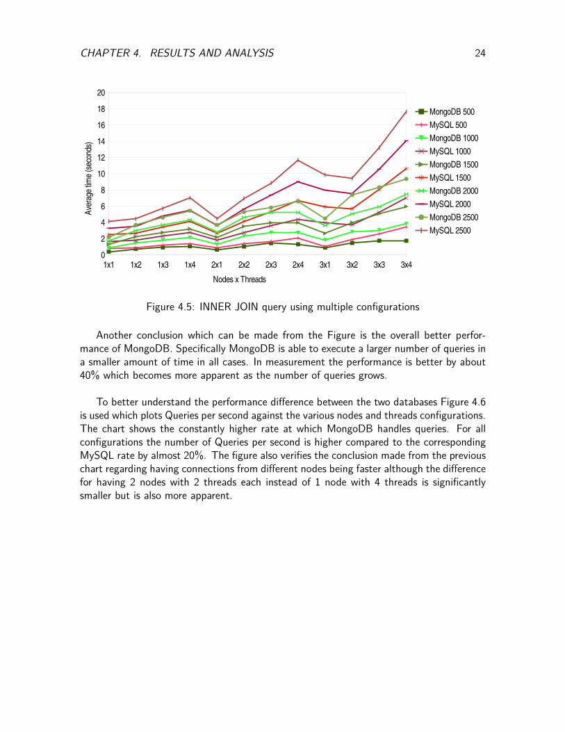
Figure 4.5: INNER JOIN query using multiple configurations
Another conclusion which can be made from the Figure is the overall better perfor-mance of MongoDB. Specifically MongoDB is able to execute a larger number of queries ina smaller amount of time in all cases. In measurement the performance is better by about40% which becomes more apparent as the number of queries grows.
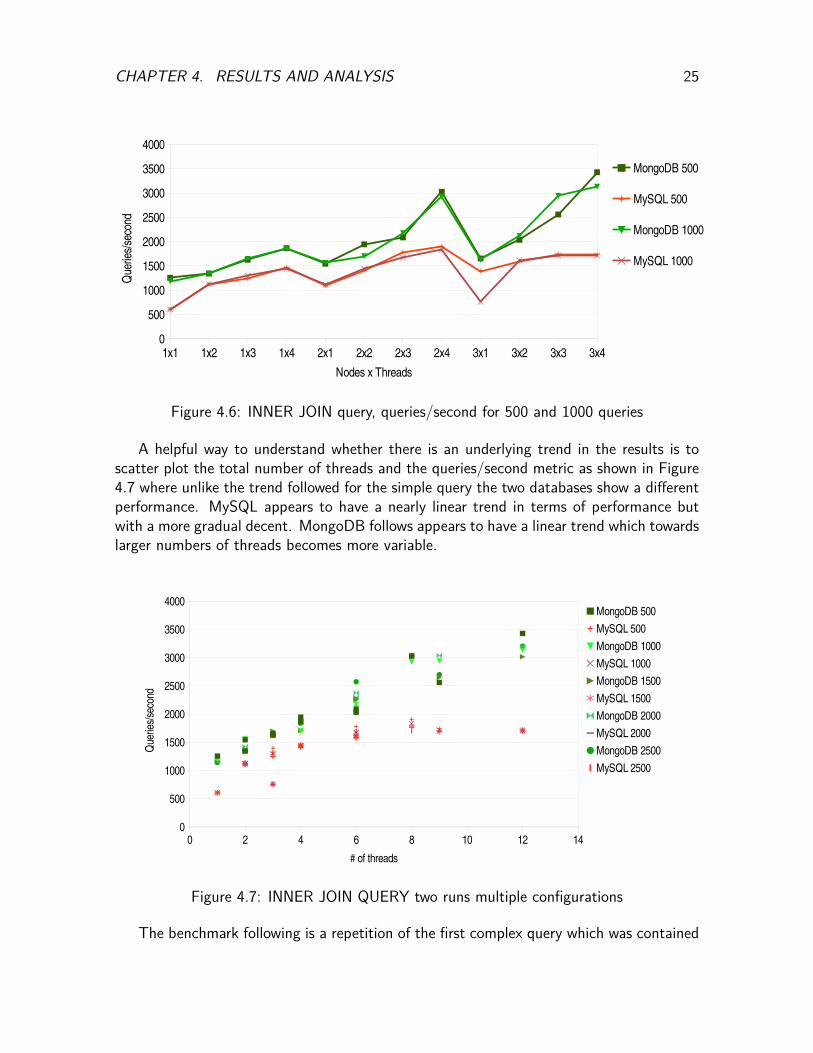
To better understand the performance difference between the two databases Figure 4.6is used which plots Queries per second against the various nodes and threads configurations.The chart shows the constantly higher rate at which MongoDB handles queries. For allconfigurations the number of Queries per second is higher compared to the correspondingMySQL rate by almost 20%. The figure also verifies the conclusion made from the previouschart regarding having connections from different nodes being faster although the differencefor having 2 nodes with 2 threads each instead of 1 node with 4 threads is significantlysmaller but is also more apparent.
CHAPTER 4. RESULTS AND ANALYSIS 25
Figure 4.6: INNER JOIN query, queries/second for 500 and 1000 queries
A helpful way to understand whether there is an underlying trend in the results is toscatter plot the total number of threads and the queries/second metric as shown in Figure4.7 where unlike the trend followed for the simple query the two databases show a differentperformance. MySQL appears to have a nearly linear trend in terms of performance butwith a more gradual decent. MongoDB follows appears to have a linear trend which towardslarger numbers of threads becomes more variable.
Figure 4.7: INNER JOIN QUERY two runs multiple configurations
The benchmark following is a repetition of the first complex query which was contained

CHAPTER 4. RESULTS AND ANALYSIS 26
an INNER JOIN operation but this uses the alternative nested SELECTs or subqueries.Figure 4.8 shows the resulting average times against the various configurations for bothMongoDB and MySQL. MySQL has an advantage over MongoDB for the majority of runsbut for the configurations of 3x2, 3x3 and 3x4 the performance is almost identical.
Figure 4.8: Nested SELECT query
To better understand the results the total queries per second chart is shown in Figure 4.9.In this chart the better performance of MySQL is clear up to 2x4 threads. Afterwards the2 databases’ becomes similar. This can be attributed to the higher number of connectionsfrom different nodes in combination with the complicated nature of the query executed.
Figure 4.9: Nested SELECT query queries/second

CHAPTER 4. RESULTS AND ANALYSIS 27
The scatter plot of queries per second against the total number of threads in Figure 4.10shows the overall declining trend of MySQL whereas MongoDB’s performance diminishesup to 6 threads and then remains relatively stable.
Figure 4.10: Nested SELECT query scatter plot
The next benchmark involving the normal MongoDB deployment was regarding a highlycomplex query with 2 INNER JOINs and a subquery. The resulting measurements for theaverage time are shown in Figure 4.11. The chart shows the performance penalty of MySQLhaving to perform such a complex query whereas the MongoDB equivalent performs muchbetter. This is attributed to the fact that MongoDB uses subdocuments instead of deployinga full database schema and thus saves time by requiring to query a smaller number ofcollections. This advantage that NoSQL databases have over RDBMSs comes at the costof data duplication resulting from a denormalised database schema.

CHAPTER 4. RESULTS AND ANALYSIS 28
Figure 4.11: 2 INNER JOINS & subquery
In Figure 4.12 the same benchmark is shown by plotting the average queries per second.MySQL appears to have a logarithmic trend which is proved by plotting the same chartusing the logarithms of the two axis. This is shown in Figure 4.13 where not only MySQLbut also MongoDB appear to have the same trend. This is unclear in the Figures 4.11 and4.12 due to large difference in the timings of MySQL which enlarge the scale. Despite thisthough MySQL still has a disadvantage due to its performance.
Figure 4.12: 2 INNER JOINS & subquery, queries per second
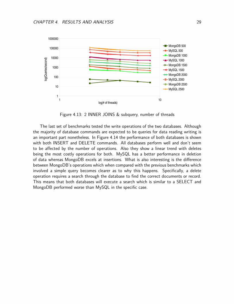
CHAPTER 4. RESULTS AND ANALYSIS 29
Figure 4.13: 2 INNER JOINS & subquery, number of threads
The last set of benchmarks tested the write operations of the two databases. Althoughthe majority of database commands are expected to be queries for data reading writing isan important part nonetheless. In Figure 4.14 the performance of both databases is shownwith both INSERT and DELETE commands. All databases perform well and don’t seemto be affected by the number of operations. Also they show a linear trend with deletesbeing the most costly operations for both. MySQL has a better performance in deletionof data whereas MongoDB excels at insertions. What is also interesting is the differencebetween MongoDB’s operations which when compared with the previous benchmarks whichinvolved a simple query becomes clearer as to why this happens. Specifically, a deleteoperation requires a search through the database to find the correct documents or record.This means that both databases will execute a search which is similar to a SELECT andMongoDB performed worse than MySQL in the specific case.

CHAPTER 4. RESULTS AND ANALYSIS 30
Figure 4.14: INSERT and DELETE operations
4.2 MongoDB ShardingThe following benchmarks were performed on the MongoDB shard deployment which wasconfigured with 3 shard nodes and a query router. These benchmarks which are shown inFigure 4.15 were done using the simple query and the complex query which in MySQL wouldbe the equivalent of having an JOIN operation. The shard configuration does not performwell with the replica configuration being faster in both cases. This can be attributed to thefact that the query router in the MongoDB shard creates an overhead instead of allowingan improvement by separating the load amongst the database nodes.

CHAPTER 4. RESULTS AND ANALYSIS 31
Figure 4.15: MongoDB Replica and Shard configurations, simple query
Figure 4.16: MongoDB Replica and Shard configurations, complex query
In Figure 4.17 the comparison the scatter plot of MongoDB shards and MySQL is shownwhen performing the complex query. The same plot but with the simple query is unnecessaryas MySQL outperformed the MongoDB replica configuration which itself was faster thanMongoDB shards. The first observation which can be mad is the close performance the twodatabases systems have. Specifically, MySQL has a linear trend which seems to becomemore steep as the total number of queries increases. MongoDB shard also follows a lineartrend but the most interesting deduction which can be made from the chart, as well as the

CHAPTER 4. RESULTS AND ANALYSIS 32
previous ones is the performance drop caused by the connections made through a singlenode instead of two, ie. 1x4 versus 2x2. This again shows the effect different connectionusage can have on MongoDB.
Figure 4.17: MongoDB Shard and MySQL, complex query
4.3 Database sizeIn order to measure the performance of the database management systems according tothe size of the database an iterative approach was considered, whereby a specific processwas repeated with only a single variable changing, in this case the variable being thedatabase size. The benchmark initially deleted all existing records from the database andrepopulated it with the required data set size. Afterwards a test was performed which wasnot recorded but it allowed to eliminate any caching issues with newly stored data whichwould disrupt subsequent measurements. The normal benchmark followed which measureda specific amount of queries. This procedure was repeated for all database sizes and themeasurement for the becnhmark with simple queries is displayed in Figure 4.18. The chartwhich is for a simple query shows a steady trend for both databases with no significantvariations as the database size increases.

CHAPTER 4. RESULTS AND ANALYSIS 33
Figure 4.18: Simple query with different database sizes
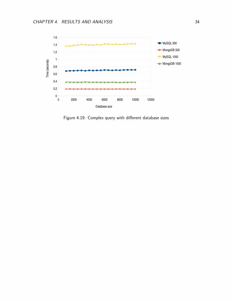
In Figure 4.19 the variation of execution time of 500 and 1000 complex queries isshown in relation to the database size. Here MongoDB has a similar performance with theprevious benchmark with no significant variations. MySQL though has a slightly diminishingperformance as time increases when the database size increases. This can be explained bythe access of two tables which although is not a linear search due to indexing the fact thatthe result of each query requires joining the data from two tables is sufficient to explainthe small performance penalty as it becomes increasingly more difficult perform searches intwo tables at the same time. Such a performance penalty may be observed in much largerdatabase sizes when performing a simple query but the penalty may be negligible. Due tothe high memory requirement of the benchmarking harness performing benchmarks whichit was unable to handle,subsequent measurements for databases with larger sizes were notperformed.
CHAPTER 4. RESULTS AND ANALYSIS 34
Figure 4.19: Complex query with different database sizes

Chapter 5
Conclusion
The project was an investigation and comparison of the performance and scaling of Re-lational Database Management Systems and NoSQL databases with the aim of exploringhow the different factors affect each database and whether on technology is more suitablethan the other and in which situations. The first database type which, relational databases,were developed with structure in mind and built on the premise of tables with rows whichfollowed a pre-specified schema. Their most important feature, the database schema whichgave a logical view of the database in combination with relations between tables allowedthe building of databases which were fast, easy to develop, and eliminated duplication ofdata but at the same time guaranteed reliability. NoSQL databases which are relatively newbecame a popular trend as they provide performance and horizontal scalability which madethem suitable for data centers requiring massive amounts of storage and the capability ofextending the database easily as no pre-defined schema exists.
The project tested, analysed and compared the performance and scalability of the twodatabase types. The experiments done included running different numbers and types ofqueries, some more complex than others, in order to analyse how the databases scaled withincreased load. The most important factor in this case was the query type used as Mon-goDB could handle more complex queries faster due mainly to its simpler schema at thesacrifice of data duplication meaning that a NoSQL database may contain large amounts ofdata duplicates. Although a schema directly migrated from the RDBMS could be used thiswould eliminate the advantage of MongoDB’s underlying data representation of subdocu-ments which allowed the use of less queries towards the database as tables were combined.Despite the performance gain which MongoDB had over MySQL in these complex queries,when the benchmark modelled the MySQL query similarly to the MongoDB complex queryby using nested SELECTs MySQL performed best although at higher numbers of connec-tions the two behaved similarly. The last type of query benchmarked which was the complexquery containing two JOINS and and a subquery showed the advantage MongoDB has overMySQL due to its use of subdocuments. This advantage comes at the cost of data du-plication which causes an increase in the database size. If such queries are typical in anapplication then it is important to consider NoSQL databases as alternatives while taking
35
CHAPTER 5. CONCLUSION 36
in account the cost in storage and memory size resulting from the larger database size.
The second type of query operations performed in the benchmarks were write oper-ations. The results from these benchmarks showed that MySQL performs better whendeleting data which is logical considering that it performs better in simple search queries.This is connected to deletion as deletion requires finding the record to be deleted first.MongoDB performed better during insertions with both databases having a linear trend inthese benchmarks.
Another important aspect of the experiments was the use of different configurations fornodes and threads. This part of the benchmarks required running the benchmarking harnesson 1, 2 and 3 nodes with multiple numbers of threads in order to test how the databasesperformed with multiple connections. This benchmark was done in conjunction with theprevious benchmark of having different query types. Depending on the query complexitythe databases behave differently but at higher numbers of connections the performance interms of queries/second appeared to converge.
As the two databases behave differently according to the type of queries used thechoice of which database to use lies on the type of application the system will be using. Inaddition it is important to consider the effect that using a database such as MongoDB willhave on the hardware storage due to the increased database size. Despite the indicationthat the performance penalty on both databases is small depending on the database sizeit is nonetheless an important factor when considering the type of queries which will beperformed by applications.
5.1 Deviations from the project planThe dissertation followed the plan drafted during Project Preparation but deviated at somepoints during the later stages in order to accommodate unexpected problems with the Mon-goDB benchmarking part. In order to address the issue the extra time which was set at theend of the plan was distributed to solve the problems. In addition, writing up started inparallel with the development and running of the benchmarking harness due to the limitedtime available and in case any further deviations were made.
Specifically the first four parts of the project according to the work plan were completedsuccessfully and within the time constraints. Subsequently the stage of implementing thedatabases was completed but it overlapped with the next stage of building the benchmark-ing harness as unexpected issues were found while configuring MySQL Cluster. The issuesincluded the difference in hostnames expected by the system when adding nodes and alsoissues with shutting down and restarting the databases in order to try different configura-tions. The problems which arose when restarting the servers were mainly due to impropershutdowns or one node being out of sync with the other nodes.

CHAPTER 5. CONCLUSION 37
The next stage which was building the harness began as planned but extended lateinto the project as unexpected problems surfaced mainly because of differences in thedocumentation of the MongoDB driver and the actual implementation. In more detail afunction regarding indexing required different arguments compared to the documentation.This caused a delay as it was considered that indexing may have a serious effect on theperformance and as the RDBMS used indexing as well its importance intensified. Otherproblems with the development of the harness were the fact that MongoDB initialises someMongoDB specific pointers to objects using its own functions and does not require dynamicallocation. This resulted in some confusion as it wasn’t clear initially which objects werebeing initialised thus requiring a MongoDB specific method to deallocate them.
In regards to the dissertation’s scope the most important objective which was the com-parison of the performance and scalability of RDBMSs against NoSQL databases was com-pleted successfully. Various queries were used to stress both databases and different con-figurations of the test harness were used in order to understand how the databases behavewhen using queries of different complexity. In addition the systems were benchmarked inregards to the database size which showed that this factor barely affects performance.
5.2 Future workAs the amount of time available for this project was relatively small the possibilities forfurther extensions and improvements are numerous. One of the most important aspectswhich can be explored are the additions of other databases for benchmarking. Especiallysince many types of NoSQL databases exist the use of a more diverse range would provideinsight as to not only how well the different databases perform but also whether they canbe used at all instead of relational databases. Also other relational databases are likelyto perform differently due to optimisations and different storage engines used. By addingmore databases the comparison between relational databases and NoSQL databases wouldbecome more objective and provide more measurements to compare the two types.
An important part of the benchmarking harness is the various queries used. Differentqueries affect the performance of each database differenty and finding how they do is es-sential in better understanding this. By being able to understand how the queries affectperformance someone wanting to use a database for a specific scope, such as queries in-volving multiple tables with JOINs, can choose the database which performs best in thatspecific situation.
Although the project gives an indication regarding how well databases cope with largenumbers of queries further work can be done by using larger clusters to test the perfor-mance. As it was shown different numbers of connections and configurations affect thebehaviour of the databases. By extending this to a larger scale a more broad investigation
CHAPTER 5. CONCLUSION 38
can be performed with more general conclusions as to this factor.
The different sizes of a database may have significant influence in ways other than theones explored in this project. An example is the complexity of the databases in terms ofnumber of tables or how a database is deployed in NoSQL databases.
The reliability of the two database types may not have been part of the project butin the future this aspect can be examined. The reason for doing so is to understandwhether increased performance and scalability by one database type over the other affectsthe reliability. Specifically, since NoSQL do not guarantee the ACID properties a middleground can be found whereby performance and scaling reach an adequate level but at thesame time the reliability of the database is guaranteed as well.

Appendix A
Benchmark Results
A.1 MongoDB
# of Queries 1 thread 2 threads 3 threads 4 threads100 0.05035 0.074801 0.0942903333 0.11524975200 0.097766 0.1502885 0.1897333333 0.22523975300 0.144763 0.22721 0.2821616667 0.33199875400 0.202356 0.3021275 0.3754526667 0.448554500 0.273659 0.376707 0.4698933333 0.55872651000 0.470587 0.75516 0.9323583333 1.10309751500 0.732803 1.1325355 1.4159336667 1.638797752000 0.960046 1.5101695 1.8931296667 2.204101252100 1.004248 1.5833975 1.978283 2.343815252300 1.094791 1.73553 2.1736936667 2.530601252500 1.186967 1.889928 2.350015 2.739965252700 1.285125 2.0533105 2.548669 2.98266925
Table A.1: MongoDB Simple Query average time, 1 node
A.2 MySQL
39
APPENDIX A. BENCHMARK RESULTS 40
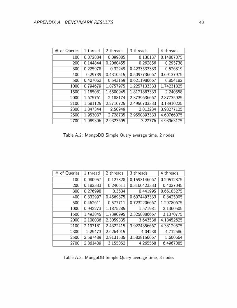
# of Queries 1 thread 2 threads 3 threads 4 threads100 0.072884 0.099085 0.130137 0.14807075200 0.144844 0.2060455 0.262856 0.295738300 0.225978 0.32249 0.4233533333 0.526319400 0.29739 0.4310515 0.5097736667 0.69137975500 0.407062 0.543159 0.6211986667 0.8541821000 0.794679 1.0757975 1.2257133333 1.742318251500 1.185081 1.6500945 1.8171883333 2.2405582000 1.675761 2.188174 2.3739636667 2.877359252100 1.681125 2.2710725 2.4950703333 3.139102252300 1.847344 2.50949 2.813234 3.982771252500 1.953037 2.728735 2.9550893333 4.607660752700 1.989396 2.9323695 3.22776 4.98963175
Table A.2: MongoDB Simple Query average time, 2 nodes
# of Queries 1 thread 2 threads 3 threads 4 threads100 0.080957 0.127828 0.1593146667 0.20512375200 0.182333 0.240611 0.3160423333 0.4027045300 0.276998 0.3634 0.441995 0.66105275400 0.332997 0.4569375 0.6074493333 0.8425005500 0.462611 0.577711 0.7232206667 1.297806751000 0.942273 1.1875285 1.571981 2.13605051500 1.493845 1.7390995 2.3258886667 3.13707752000 2.108036 2.3059335 3.643536 4.184526252100 2.197181 2.4322415 3.9224356667 4.381295752300 2.25473 2.6264015 4.04238 4.7125862500 2.587489 2.9131535 3.5828156667 5.6006642700 2.861409 3.155052 4.265568 6.4967085
Table A.3: MongoDB Simple Query average time, 3 nodes

APPENDIX A. BENCHMARK RESULTS 41
# of Queries 1 thread 2 threads 3 threads 4 threads100 0.050526 0.147696 0.183089 0.22382425200 0.129832 0.2953615 0.3669853333 0.438745300 0.219269 0.4463085 0.5453056667 0.654373400 0.307257 0.5933595 0.7333143333 0.8804445500 0.397736 0.7430275 0.922133 1.071544751000 0.841227 1.488597 1.8211506667 2.1445651500 1.294182 2.2384495 2.7625996667 3.219980752000 1.731686 2.9950495 3.7085433333 4.3355572100 1.826487 3.109542 3.866582 4.5603642300 2.017345 3.3966215 4.2568256667 4.96639352500 2.188028 3.6900805 4.60522 5.442347252700 2.362815 3.9834745 4.9965503333 5.805082
Table A.4: MongoDB Complex Query 1.1 average time, 1 node
# of Queries 1 thread 2 threads 3 threads 4 threads100 0.078912 0.2174985 0.2290246667 0.34936425200 0.227197 0.4295095 0.5054376667 0.5658265300 0.37874 0.652467 0.85488 0.81999975400 0.552387 0.790616 1.0531843333 1.04738500 0.646774 1.0272245 1.4371743333 1.32147351000 1.278552 2.3485735 2.7555153333 2.73522751500 2.186346 3.515762 3.9589636667 3.984859752000 2.809115 4.6391115 5.219248 5.253470752100 3.024854 4.8066975 5.421256 5.475085752300 3.603725 4.9771635 5.5982563333 5.986112500 3.698275 5.2832795 5.8270666667 6.5853862700 3.247461 5.4177675 6.4387053333 7.11697425
Table A.5: MongoDB Complex Query 1.1 average time, 2 nodes

APPENDIX A. BENCHMARK RESULTS 42
# of Queries 1 thread 2 threads 3 threads 4 threads100 0.215255 0.371047 0.499763 0.66309875200 0.430895 0.7453935 1.0258483333 1.37526975300 0.656353 1.1197965 1.501206 2.048496400 0.859615 1.510125 2.0908353333 2.70110475500 1.074603 1.873236 2.5834286667 3.4642111000 3.941992 3.720005 5.2496626667 7.00689851500 5.948298 5.7065595 8.0305213333 10.63563052000 7.983516 7.5759075 10.56764 14.068994752100 8.418224 8.02625 11.1193646667 14.822738752300 9.298858 8.6862925 12.1055416667 16.159046252500 9.863524 9.4254715 13.1997393333 17.638542752700 8.742225 10.230226 14.0493186667 18.98359175
Table A.6: MongoDB Complex Query 1.1 average time, 3 nodes
# of Queries 1 thread 2 threads 3 threads 4 threads100 0.080393 0.1168715 0.1647213333 0.195534200 0.150465 0.232192 0.318468 0.41097425300 0.229106 0.352806 0.4842546667 0.6369915400 0.316948 0.4775145 0.6612903333 0.8365465500 0.414129 0.588893 0.8303646667 1.055048751000 0.776958 1.1704395 1.663416 2.112252751500 1.286811 1.7676875 2.376884 3.166908252000 1.723527 2.3641295 3.2713196667 4.2570032100 1.756042 2.437629 3.5009043333 4.331882252300 1.929536 2.7019305 3.6830543333 4.855774252500 2.113822 2.9521375 4.0170063333 5.252173252700 2.223446 3.152064 4.468722 5.65689275
Table A.7: MongoDB Complex Query 1.2 average time, 1 node

APPENDIX A. BENCHMARK RESULTS 43
# of Queries 1 thread 2 threads 3 threads 4 threads100 0.10911 0.1797775 0.2081716667 0.27008425200 0.225294 0.411644 0.478181 0.64342325300 0.337303 0.6055115 0.614586 0.85738225400 0.460735 0.672302 0.941283 1.19771500 0.622098 0.8453025 1.0813196667 1.43936851000 1.21275 1.707435 2.2559476667 2.9471131500 1.803349 2.710437 3.5871243333 5.01851452000 2.469281 3.658327 4.8133753333 6.726620752100 2.677006 3.9482585 5.018753 6.9853362300 2.838046 4.36349 5.8737736667 7.3508172500 3.069688 4.578081 6.526868 7.672564252700 2.973248 4.6690235 6.7771093333 8.2895225
Table A.8: MongoDB Complex Query 1.2 average time, 2 nodes
# of Queries 1 thread 2 threads 3 threads 4 threads100 0.136032 0.223319 0.312389 0.43331525200 0.331645 0.4696665 0.7638783333 0.98583925300 0.511923 0.5745345 0.924682 1.45846425400 0.609514 0.8365365 1.227705 1.9599605500 0.755289 1.0066945 1.6918066667 2.4679191000 1.517494 2.3093185 3.8895786667 5.25739751500 2.331923 3.8123925 5.408842 7.825856752000 3.245686 5.3170795 7.8764203333 10.86763152100 3.362951 5.3938585 7.148951 11.311044252300 3.807893 5.712998 8.1956793333 12.07614852500 4.017699 6.021579 9.260337 13.334939252700 4.277297 6.0331395 9.8787476667 14.0225775
Table A.9: MongoDB Complex Query 1.2 average time, 3 nodes

APPENDIX A. BENCHMARK RESULTS 44
# of Queries 1 thread 2 threads 3 threads 4 threads100 0.061421 0.231165 0.290309 0.34301925200 0.203652 0.4744265 0.5767286667 0.680468300 0.337207 0.7198445 0.868374 1.02805675400 0.47735 0.96294 1.1710863333 1.37168925500 0.633231 1.196814 1.4644186667 1.705620751000 1.325132 2.4163135 2.9124326667 3.4064361500 2.060693 3.6323355 4.358838 5.079362752000 2.755321 4.8103525 5.873472 6.799622752100 2.90612 5.053776 6.1517153333 7.1648632300 3.202521 5.553501 6.760138 7.796669752500 3.48786 6.0176825 7.3284903333 8.485933752700 3.774195 6.526532 7.9316666667 9.1299555
Table A.10: MongoDB Complex Query 2 average time, 1 node
# of Queries 1 thread 2 threads 3 threads 4 threads100 0.087263 0.343942 0.3955633333 0.419485200 0.347202 0.6618705 0.7332733333 0.808704300 0.602966 0.999728 1.089874 1.31307575400 0.848935 1.429643 1.4354313333 1.68168725500 1.037088 1.7503155 1.7463206667 2.239410251000 2.441934 3.3056205 3.5624033333 4.2190771500 3.786181 4.984063 5.2961383333 6.1728392000 5.14681 6.7231615 7.1853886667 8.29902652100 5.256668 7.1710975 7.6076033333 8.619329252300 5.804121 8.140611 8.4075943333 9.43459152500 6.595318 8.9809205 9.035602 10.47224452700 6.281738 9.6164965 9.486774 11.27073675
Table A.11: MongoDB Complex Query 2 average time, 2 nodes

APPENDIX A. BENCHMARK RESULTS 45
# of Queries 1 thread 2 threads 3 threads 4 threads100 0.057458 0.061674 0.082752 0.10024275200 0.113917 0.114558 0.1600176667 0.196732300 0.171563 0.177839 0.2458713333 0.29511725400 0.228046 0.2300545 0.3177706667 0.3943075500 0.291688 0.2865785 0.4106786667 0.488907251000 0.573398 0.578496 0.8191866667 0.953861251500 0.848657 0.885095 1.2006263333 1.42892752000 1.136185 1.14509 1.6596243333 1.878100252100 1.185663 1.190022 1.7288023333 1.9575492300 1.310109 1.3139195 1.8203516667 2.196750252500 1.417835 1.440846 2.025522 2.324652700 1.524579 1.527794 2.228788 2.55002825
Table A.12: MySQL Simple Query average time, 1 node
# of Queries 1 thread 2 threads 3 threads 4 threads100 0.072884 0.099085 0.130137 0.14807075200 0.144844 0.2060455 0.262856 0.295738300 0.225978 0.32249 0.4233533333 0.526319400 0.29739 0.4310515 0.5097736667 0.69137975500 0.407062 0.543159 0.6211986667 0.8541821000 0.794679 1.0757975 1.2257133333 1.742318251500 1.185081 1.6500945 1.8171883333 2.2405582000 1.675761 2.188174 2.3739636667 2.877359252100 1.681125 2.2710725 2.4950703333 3.139102252300 1.847344 2.50949 2.813234 3.982771252500 1.953037 2.728735 2.9550893333 4.607660752700 1.989396 2.9323695 3.22776 4.98963175
Table A.13: MySQL Simple Query average time, 2 nodes

APPENDIX A. BENCHMARK RESULTS 46
# of Queries 1 thread 2 threads 3 threads 4 threads100 0.084 0.1393085 0.1759423333 0.238261200 0.151647 0.2944145 0.3608253333 0.468403300 0.22147 0.3998765 0.5514316667 0.658146400 0.292908 0.537042 0.7227463333 0.864767500 0.366257 0.632505 0.9331723333 1.05916551000 1.325605 1.362591 1.6702823333 2.1412341500 1.927019 2.017488 2.5509003333 3.18576952000 2.594995 2.6560925 3.4424663333 4.335933252100 2.825633 2.711552 3.3977276667 4.49956452300 2.960555 3.163766 3.7804506667 4.879685252500 3.236498 3.341857 3.985407 5.2232262700 3.123149 3.6664755 4.4574293333 5.64654175
Table A.14: MySQL Simple Query average time, 3 nodes
# of Queries 1 thread 2 threads 3 threads 4 threads100 0.162953 0.2390285 0.2319773333 0.28192075200 0.326054 0.3588795 0.4587226667 0.56699375300 0.489187 0.538394 0.6960813333 0.8192115400 0.654635 0.6948575 0.917683 1.16042525500 0.819795 0.887315 1.2090436667 1.3646751000 1.641447 1.775193 2.30831 2.77814251500 2.47847 2.653788 3.4445493333 4.137390252000 3.305032 3.5608375 4.8113383333 5.5349632100 3.470025 3.7006245 4.880723 5.9157942300 3.804865 4.1072415 5.2554666667 6.37064652500 4.136924 4.42951 5.724727 7.0134552700 4.474203 4.7103945 6.2331216667 7.5139345
Table A.15: MySQL Complex Query 1.1 average time, 1 node

APPENDIX A. BENCHMARK RESULTS 47
# of Queries 1 thread 2 threads 3 threads 4 threads100 0.183805 0.325291 0.314581 0.35671575200 0.373505 0.614633 0.6772796667 0.83709325300 0.539237 0.9292885 1.038387 1.22201675400 0.697565 1.2794935 1.324781 1.74812500 0.915612 1.413485 1.686512 2.100378751000 1.789728 2.769948 3.5846636667 4.360936251500 2.658399 4.156596 5.3436446667 6.6900462000 3.576829 5.6412465 7.391638 9.0515572100 3.722857 5.849565 7.3606406667 9.4303022300 4.093636 6.311247 7.9748973333 10.1544942500 4.470268 6.9644455 8.8771803333 11.695124752700 4.842984 7.716159 9.8059606667 12.30326075
Table A.16: MySQL Complex Query 1.1 average time, 2 nodes
# of Queries 1 thread 2 threads 3 threads 4 threads100 0.215255 0.371047 0.499763 0.66309875200 0.430895 0.7453935 1.0258483333 1.37526975300 0.656353 1.1197965 1.501206 2.048496400 0.859615 1.510125 2.0908353333 2.70110475500 1.074603 1.873236 2.5834286667 3.4642111000 3.941992 3.720005 5.2496626667 7.00689851500 5.948298 5.7065595 8.0305213333 10.63563052000 7.983516 7.5759075 10.56764 14.068994752100 8.418224 8.02625 11.1193646667 14.822738752300 9.298858 8.6862925 12.1055416667 16.159046252500 9.863524 9.4254715 13.1997393333 17.638542752700 8.742225 10.230226 14.0493186667 18.98359175
Table A.17: MySQL Complex Query 1.1 average time, 3 nodes
APPENDIX A. BENCHMARK RESULTS 48
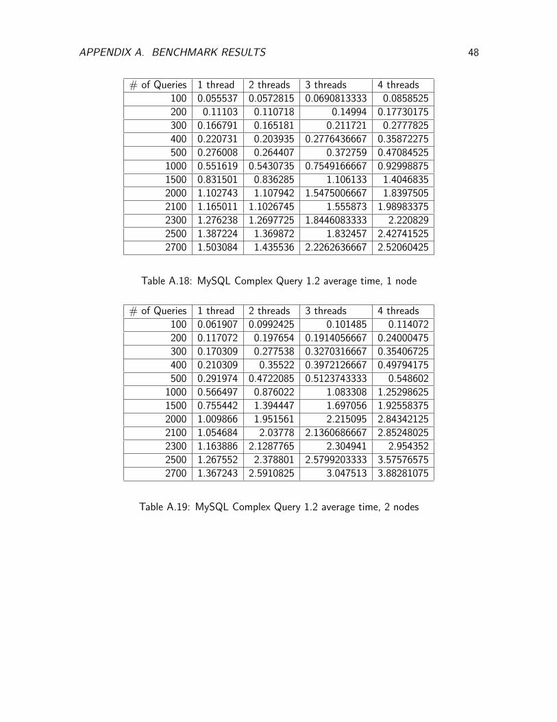
# of Queries 1 thread 2 threads 3 threads 4 threads100 0.055537 0.0572815 0.0690813333 0.0858525200 0.11103 0.110718 0.14994 0.17730175300 0.166791 0.165181 0.211721 0.2777825400 0.220731 0.203935 0.2776436667 0.35872275500 0.276008 0.264407 0.372759 0.470845251000 0.551619 0.5430735 0.7549166667 0.929988751500 0.831501 0.836285 1.106133 1.40468352000 1.102743 1.107942 1.5475006667 1.83975052100 1.165011 1.1026745 1.555873 1.989833752300 1.276238 1.2697725 1.8446083333 2.2208292500 1.387224 1.369872 1.832457 2.427415252700 1.503084 1.435536 2.2262636667 2.52060425
Table A.18: MySQL Complex Query 1.2 average time, 1 node
# of Queries 1 thread 2 threads 3 threads 4 threads100 0.061907 0.0992425 0.101485 0.114072200 0.117072 0.197654 0.1914056667 0.24000475300 0.170309 0.277538 0.3270316667 0.35406725400 0.210309 0.35522 0.3972126667 0.49794175500 0.291974 0.4722085 0.5123743333 0.5486021000 0.566497 0.876022 1.083308 1.252986251500 0.755442 1.394447 1.697056 1.925583752000 1.009866 1.951561 2.215095 2.843421252100 1.054684 2.03778 2.1360686667 2.852480252300 1.163886 2.1287765 2.304941 2.9543522500 1.267552 2.378801 2.5799203333 3.575765752700 1.367243 2.5910825 3.047513 3.88281075
Table A.19: MySQL Complex Query 1.2 average time, 2 nodes

APPENDIX A. BENCHMARK RESULTS 49
# of Queries 1 thread 2 threads 3 threads 4 threads100 0.069579 0.121272 0.172381 0.21339725200 0.152236 0.2436895 0.3343893333 0.41959675300 0.216267 0.3746485 0.4850456667 0.669093400 0.284336 0.5075365 0.635755 0.9839555500 0.352012 0.6592525 0.7719553333 1.145915751000 1.23672 1.259257 1.657809 2.2843121500 1.821226 1.847769 2.4361673333 3.4224062000 2.418525 2.502922 3.280702 4.4742082100 2.662663 2.7220145 3.6390203333 4.7003192300 3.091954 2.8501815 3.95598 5.3004352500 3.023243 3.1110105 4.3960646667 5.619908252700 2.76028 3.3580175 4.8631396667 6.2929215
Table A.20: MySQL Complex Query 1.2 average time, 3 nodes
Table A.21: INSERT and DELETE
# of commands MySQL INSERT MongoDB INSERT MySQL DELETE MongoDB DELETE100 0.152528 0.050925 0.163032 0.192994500 0.756668 0.277134 0.813595 0.8572931000 1.547805 0.543094 1.729822 1.7940745000 7.978989 2.832491 8.52242 10.28844710000 15.935719 5.731883 17.499579 21.51904150000 82.883779 32.321015 90.492908 114.414941

Appendix B
Configuration and Scripts
B.1 MongoDBCreate configuration directories for each server. Here the directory /data will contain theconfiguration directories for each server. Run the mongod replica servers:
/MONGODB_DIRECTORY/mongod −−dbpath ~/ data / con f i gdb1−−po r t 27017 −−r e p l S e t s e r v e r 1 /
. /mongod −−dbpath ~/ data / con f i gdb2 −−po r t 27018−−r e p l S e t s e r v e r 1 /
Run arbiter server:. / mongod −−dbpath ~/ data / a r b i t e r −−po r t 27019 −−r e p l S e t s e r v e r 1 /
Run mongo shell and initiate configuration:$ . /mongoMongoDB s h e l l v e r s i o n : 2 . 2 . 3conne c t i n g to : t e s t> r s . i n i t i a t e ({" _id " : " s e r v e r 1 " , "members " : [. . . {" _id " : 0 , " hos t " : " compute −0−1:27017"} ,. . . {" _id " : 1 , " hos t " : " compute −0−2:27018"} ,. . . {" _id " : 2 , " hos t " : " compute −0−1:27019" ,. . . " a r b i t e rO n l y " : " t r u e " } ] } )
All servers, including arbiter, need to use the same hostname terminology, ie, compute-0-1:27017 compute-0-2:27018 or localhost:27017 localhost:27018 Check the set from themongo shell
s e r v e r 1 :STARTUP2> db . i sMa s t e r ( ){
" setName " : " s e r v e r 1 " ," i sma s t e r " : t rue ," s e conda r y " : f a l s e ,
50

APPENDIX B. CONFIGURATION AND SCRIPTS 51
" ho s t s " : [" compute −0−1:27017" ," compute −0−2:27018"
] ," a r b i t e r s " : [
" compute −0−1:27019"] ," p r ima ry " : " compute −0−1:27017" ,"me" : " compute −0−1:27017" ," maxBsonObjectS ize " : 16777216 ," l o ca lT ime " : ISODate ("2013−07−07T05 : 2 0 : 1 9 . 3 0 8Z" ) ," ok " : 1
}
B.2 MySQL ClusterTo setup MySQL Cluster:
• Download the generic version from http://www.mysql.com/downloads/cluster/usingwget on one of the compute nodes.
• Follow the quickstart guide provided http://downloads.mysql.com/tutorials/cluster/mysql_wp_cluster_quickstart_linux.pdf(alsoavailable on this page as an attachment), but use the following configuration:
– For the Management Node (ndb_mgmd) - set the hostname to the hostnameof the node which will manage the cluster. In this case compute-0-1 was used.
– For the other 2 nodes (ndbd) the appropriate hostnames must be used whichshould be different than the Mananagement Node’s. In this case compute-0-2and compute-0-3.
– The step of initialising the nodes must be executed on the nodes themselvesand instead of localhost the hostname of the Management Node must be used,ie. user@compute-0-3 ]HOME/mysqlc/bin/ndbd -c compute-0-1:1186
– The status check of the cluster should again be done from the ManagementNode as well as the initialisation of the MySQL server.
Note: The version of MySQL Cluster used is 7.2.10 64bits.
B.3 Harness
B.3.1 BuildingTo compile the benchmark first the necessary MySQL and MongoDB drivers need to beinstalled which can be retrieved from the following websites:

APPENDIX B. CONFIGURATION AND SCRIPTS 52
http://www.mysql.com/products/connector/ https://github.com/mongodb/mongo-c-driver
Each driver contains instructions on how to build it. After building the drivers theheader files from each driver’s include directory need to be copied in the system’s includedirectory, usually /usr/include. The library files which are compiled also need to be copiedto the corresponding system library directory, usually /usr/lib. Next as root run:
depmod -a
To compile the application inside the source code directory simply run:
make
B.3.2 RUNNINGTo run and see the available options:
./harness -?
Available options are:
−o,−−output F i l e to w r i t e output to−i ,−− i t e r a t i o n s Number o f q u e r i e s to pe r fo rm
f o r each t e s t , 500−1000000
−t ,−− t e s t I t e r a t i o n s Number o f t e s t s , 1−100−r ,−−random 0 |1 Use random s t r i n g s f o r da tabase
p opu l a t i n g−d,−−database Database to pe r fo rm t e s t on ,
0=MySQL, 1=MongoDB , 2−Both
−m,−−h o s t s q l MySQL database hostname−n,−−hostno MongoDB database hostname−s ,−− s q l p o r t MySQL database po r t−q,−−mongoport MongoDB database po r t
B.4 Parallel Shell Script
Listing B.1: Parallel execution script#!/ b i n / bashcd $HOME/ t e s t s
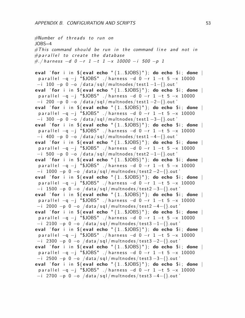
APPENDIX B. CONFIGURATION AND SCRIPTS 53
#Number o f t h r e a d s to run onJOBS=4#This command shou l d be run i n the command l i n e and not i n#p a r a l l e l to c r e a t e the da tabase#./ ha r n e s s −d 0 −r 1 −t 1 −x 10000 − i 500 −p 1
eval ’ fo r i i n $ ( eval echo " { 1 . . $JOBS}" ) ; do echo $ i ; done |p a r a l l e l −q − j "$JOBS" . / ha r n e s s −d 0 −r 1 −t 5 −x 10000
− i 100 −p 0 −o / data / s q l /mul tnodes / t e s t 1 −1−{}.out ’eval ’ fo r i i n $ ( eval echo " { 1 . . $JOBS}" ) ; do echo $ i ; done |p a r a l l e l −q − j "$JOBS" . / ha r n e s s −d 0 −r 1 −t 5 −x 10000
− i 200 −p 0 −o / data / s q l /mul tnodes / t e s t 1 −2−{}.out ’eval ’ fo r i i n $ ( eval echo " { 1 . . $JOBS}" ) ; do echo $ i ; done |p a r a l l e l −q − j "$JOBS" . / ha r n e s s −d 0 −r 1 −t 5 −x 10000
− i 300 −p 0 −o / data / s q l /mul tnodes / t e s t 1 −3−{}.out ’eval ’ fo r i i n $ ( eval echo " { 1 . . $JOBS}" ) ; do echo $ i ; done |p a r a l l e l −q − j "$JOBS" . / ha r n e s s −d 0 −r 1 −t 5 −x 10000
− i 400 −p 0 −o / data / s q l /mul tnodes / t e s t 1 −4−{}.out ’eval ’ fo r i i n $ ( eval echo " { 1 . . $JOBS}" ) ; do echo $ i ; done |p a r a l l e l −q − j "$JOBS" . / ha r n e s s −d 0 −r 1 −t 5 −x 10000
− i 500 −p 0 −o / data / s q l /mul tnodes / t e s t 2 −1−{}.out ’eval ’ fo r i i n $ ( eval echo " { 1 . . $JOBS}" ) ; do echo $ i ; done |p a r a l l e l −q − j "$JOBS" . / ha r n e s s −d 0 −r 1 −t 5 −x 10000
− i 1000 −p 0 −o / data / s q l /mul tnodes / t e s t 2 −2−{}.out ’eval ’ fo r i i n $ ( eval echo " { 1 . . $JOBS}" ) ; do echo $ i ; done |p a r a l l e l −q − j "$JOBS" . / ha r n e s s −d 0 −r 1 −t 5 −x 10000
− i 1500 −p 0 −o / data / s q l /mul tnodes / t e s t 2 −3−{}.out ’eval ’ fo r i i n $ ( eval echo " { 1 . . $JOBS}" ) ; do echo $ i ; done |p a r a l l e l −q − j "$JOBS" . / ha r n e s s −d 0 −r 1 −t 5 −x 10000
− i 2000 −p 0 −o / data / s q l /mul tnodes / t e s t 2 −4−{}.out ’eval ’ fo r i i n $ ( eval echo " { 1 . . $JOBS}" ) ; do echo $ i ; done |p a r a l l e l −q − j "$JOBS" . / ha r n e s s −d 0 −r 1 −t 5 −x 10000
− i 2100 −p 0 −o / data / s q l /mul tnodes / t e s t 3 −1−{}.out ’eval ’ fo r i i n $ ( eval echo " { 1 . . $JOBS}" ) ; do echo $ i ; done |p a r a l l e l −q − j "$JOBS" . / ha r n e s s −d 0 −r 1 −t 5 −x 10000
− i 2300 −p 0 −o / data / s q l /mul tnodes / t e s t 3 −2−{}.out ’eval ’ fo r i i n $ ( eval echo " { 1 . . $JOBS}" ) ; do echo $ i ; done |p a r a l l e l −q − j "$JOBS" . / ha r n e s s −d 0 −r 1 −t 5 −x 10000
− i 2500 −p 0 −o / data / s q l /mul tnodes / t e s t 3 −3−{}.out ’eval ’ fo r i i n $ ( eval echo " { 1 . . $JOBS}" ) ; do echo $ i ; done |p a r a l l e l −q − j "$JOBS" . / ha r n e s s −d 0 −r 1 −t 5 −x 10000
− i 2700 −p 0 −o / data / s q l /mul tnodes / t e s t 3 −4−{}.out ’
Bibliography
[1] Berg K., Seymour T., and Coel R. History of Databases. International Journal ofManagement and Information Services, 17, 2013.
[2] MongoDB. MongoDB Manual. http://docs.mongodb.org/manual/. Accessed:15-08-2013.
[3] Smith G., Robert T., and Browne C. Tuning Your PostegreSQL Server. http://wiki.postgresql.org/wiki/Tuning_Your_PostgreSQL_Server. Accessed: 14-08-2013.
[4] Apache. Cassandra Wiki: Getting Started. http://wiki.apache.org/cassandra/GettingStarted. Accessed: 14-08-2013.
[5] Apache. Apache CouchDB Manual. http://docs.couchdb.org/en/latest/. Ac-cessed: 14-08-2013.
[6] Beynon-Davies P. Database Systems. Palgrave Macmillan, 3rd edition.
[7] Strozzi C. NoSQL: a Non-SQL RDBMS. http://www.strozzi.it/cgi-bin/CSA/tw7/I/en_US/nosql/Home%20Page.
[8] Strauch C. NoSQL Databases.
[9] Batra S. and Tyagi C. Comparative Analysis of Relational And Graph Databases.International Journal of Soft Computing and Engineering (IJSCE), 2(2), May 2012.ISSN: 2231 2307.
[10] Kemme B., Jimenez-Peris R., and Patino-Martinez M. Database Repli-cation. Synthesis Lectures on Data Management, page 17, 2010.doi:10.2200/S00296ED1V01Y201008DTM007.
[11] Oracle Corporation. Differences between the NDB and InnoDB Storage Engines. http://dev.mysql.com/doc/refman/5.1/en/mysql-cluster-ndb-innodb-engines.html. Accessed: 14-08-2013.
[12] EPCC. EDIM1: Data Intensive Machine. http://www.epcc.ed.ac.uk/facilities/other-facilities/edim1-data-intensive-machine. Accessed:14-08-2013.
54

BIBLIOGRAPHY 55
[13] Rocks Group. Rocks: Open Source Toolkit Real and Virtual Clusters. http://www.rocksclusters.org/wordpress/. Accessed: 13-08-2013.
[14] Free Software Foundation. GNU parallel. http://www.gnu.org/software/parallel/. Accessed: 13-08-2013.
[15] Oracle Corporation. MySQL Manual: The Slow Query Log. http://dev.mysql.com/doc/refman/5.1/en/slow-query-log.html. Accessed: 14-08-2013.


