RDF2Vec: RDF Graph Embeddings for Data Mining Petar Ristoski, Heiko Paulheim Data and Web Science Group, University of Mannheim, Germany {petar.ristoski,heiko}@informatik.uni-mannheim.de Abstract. Linked Open Data has been recognized as a valuable source for background information in data mining. However, most data mining tools require features in propositional form, i.e., a vector of nominal or numerical features associated with an instance, while Linked Open Data sources are graphs by nature. In this paper, we present RDF2Vec, an ap- proach that uses language modeling approaches for unsupervised feature extraction from sequences of words, and adapts them to RDF graphs. We generate sequences by leveraging local information from graph sub- structures, harvested by Weisfeiler-Lehman Subtree RDF Graph Kernels and graph walks, and learn latent numerical representations of entities in RDF graphs. Our evaluation shows that such vector representations out- perform existing techniques for the propositionalization of RDF graphs on a variety of different predictive machine learning tasks, and that fea- ture vector representations of general knowledge graphs such as DBpedia and Wikidata can be easily reused for different tasks. Keywords: Graph Embeddings, Linked Open Data, Data Mining 1 Introduction Linked Open Data (LOD) [29] has been recognized as a valuable source of back- ground knowledge in many data mining tasks and knowledge discovery in general [25]. Augmenting a dataset with features taken from Linked Open Data can, in many cases, improve the results of a data mining problem at hand, while exter- nalizing the cost of maintaining that background knowledge [18]. Most data mining algorithms work with a propositional feature vector rep- resentation of the data, i.e., each instance is represented as a vector of features hf 1 ,f 2 , ..., f n i, where the features are either binary (i.e., f i ∈{true, false}), nu- merical (i.e., f i ∈ R), or nominal (i.e., f i ∈ S, where S is a finite set of symbols). LOD, however, comes in the form of graphs, connecting resources with types and relations, backed by a schema or ontology. Thus, for accessing LOD with existing data mining tools, transformations have to be performed, which create propositional features from the graphs in LOD, i.e., a process called propositionalization [10]. Usually, binary features (e.g., true if a type or relation exists, false otherwise) or numerical features
Transcript
RDF2Vec: RDF Graph Embeddingsfor Data Mining
Petar Ristoski, Heiko Paulheim
Data and Web Science Group, University of Mannheim, Germany{petar.ristoski,heiko}@informatik.uni-mannheim.de
Abstract. Linked Open Data has been recognized as a valuable sourcefor background information in data mining. However, most data miningtools require features in propositional form, i.e., a vector of nominal ornumerical features associated with an instance, while Linked Open Datasources are graphs by nature. In this paper, we present RDF2Vec, an ap-proach that uses language modeling approaches for unsupervised featureextraction from sequences of words, and adapts them to RDF graphs.We generate sequences by leveraging local information from graph sub-structures, harvested by Weisfeiler-Lehman Subtree RDF Graph Kernelsand graph walks, and learn latent numerical representations of entities inRDF graphs. Our evaluation shows that such vector representations out-perform existing techniques for the propositionalization of RDF graphson a variety of different predictive machine learning tasks, and that fea-ture vector representations of general knowledge graphs such as DBpediaand Wikidata can be easily reused for different tasks.
Keywords: Graph Embeddings, Linked Open Data, Data Mining
1 Introduction
Linked Open Data (LOD) [29] has been recognized as a valuable source of back-ground knowledge in many data mining tasks and knowledge discovery in general[25]. Augmenting a dataset with features taken from Linked Open Data can, inmany cases, improve the results of a data mining problem at hand, while exter-nalizing the cost of maintaining that background knowledge [18].
Most data mining algorithms work with a propositional feature vector rep-resentation of the data, i.e., each instance is represented as a vector of features〈f1, f2, ..., fn〉, where the features are either binary (i.e., fi ∈ {true, false}), nu-merical (i.e., fi ∈ R), or nominal (i.e., fi ∈ S, where S is a finite set of symbols).LOD, however, comes in the form of graphs, connecting resources with types andrelations, backed by a schema or ontology.
Thus, for accessing LOD with existing data mining tools, transformationshave to be performed, which create propositional features from the graphs inLOD, i.e., a process called propositionalization [10]. Usually, binary features(e.g., true if a type or relation exists, false otherwise) or numerical features
(e.g., counting the number of relations of a certain type) are used [20, 24]. Othervariants, e.g., counting different graph sub-structures are possible [34].
In this work, we adapt language modeling approaches for latent represen-tation of entities in RDF graphs. To do so, we first convert the graph into aset of sequences of entities using two different approaches, i.e., graph walks andWeisfeiler-Lehman Subtree RDF graph kernels. In the second step, we use thosesequences to train a neural language model, which estimates the likelihood ofa sequence of entities appearing in a graph. Once the training is finished, eachentity in the graph is represented as a vector of latent numerical features.
Projecting such latent representations of entities into a lower dimensionalfeature space shows that semantically similar entities appear closer to each other.We use several RDF graphs and data mining datasets to show that such latentrepresentation of entities have high relevance for different data mining tasks.
The generation of the entities’ vectors is task and dataset independent, i.e.,once the vectors are generated, they can be used for any given task and any ar-bitrary algorithm, e.g., SVM, Naive Bayes, Random Forests, Neural Networks,KNN, etc. Also, since all entities are represented in a low dimensional featurespace, building machine learning models becomes more efficient. To foster thereuse of the created feature sets, we provide the vector representations of DB-pedia and Wikidata entities as ready-to-use files for download.
The rest of this paper is structured as follows. In Section 2, we give anoverview of related work. In Section 3, we introduce our approach, followed byan evaluation in section Section 4. We conclude with a summary and an outlookon future work.
2 Related Work
In the recent past, a few approaches for generating data mining features fromLinked Open Data have been proposed. Many of those approaches are supervised,i.e., they let the user formulate SPARQL queries, and a fully automatic featuregeneration is not possible. LiDDM [8] allows the users to declare SPARQL queriesfor retrieving features from LOD that can be used in different machine learningtechniques. Similarly, Cheng et al. [3] propose an approach feature generationafter which requires the user to specify SPARQL queries. A similar approachhas been used in the RapidMiner1 semweb plugin [9], which preprocesses RDFdata in a way that it can be further processed directly in RapidMiner. Mynarzet al. [16] have considered using user specified SPARQL queries in combinationwith SPARQL aggregates.
FeGeLOD [20] and its successor, the RapidMiner Linked Open Data Exten-sion [23], have been the first fully automatic unsupervised approach for enrichingdata with features that are derived from LOD. The approach uses six differentunsupervised feature generation strategies, exploring specific or generic relations.It has been shown that such feature generation strategies can be used in manydata mining tasks [21, 23].
1 http://www.rapidminer.com/
A similar problem is handled by Kernel functions, which compute the dis-tance between two data instances by counting common substructures in thegraphs of the instances, i.e. walks, paths and trees. In the past, many graphkernels have been proposed that are tailored towards specific applications [7], ortowards specific semantic representations [5]. Only a few approaches are generalenough to be applied on any given RDF data, regardless the data mining task.Losch et al. [12] introduce two general RDF graph kernels, based on intersec-tion graphs and intersection trees. Later, the intersection tree path kernel wassimplified by Vries et al. [33]. In another work, Vries et al. [32, 34] introduce anapproximation of the state-of-the-art Weisfeiler-Lehman graph kernel algorithmaimed at improving the computation time of the kernel when applied to RDF.Furthermore, the kernel implementation allows for explicit calculation of theinstances’ feature vectors, instead of pairwise similarities.
Our work is closely related to the approaches DeepWalk [22] and Deep GraphKernels [35]. DeepWalk uses language modeling approaches to learn social repre-sentations of vertices of graphs by modeling short random-walks on large socialgraphs, like BlogCatalog, Flickr, and YouTube. The Deep Graph Kernel ap-proach extends the DeepWalk approach, by modeling graph substructures, likegraphlets, instead of random walks. The approach we propose in this paper dif-fers from these two approaches in several aspects. First, we adapt the languagemodeling approaches on directed labeled RDF graphs, compared to the undi-rected graphs used in the approaches. Second, we show that task-independententity vectors can be generated on large-scale knowledge graphs, which later canbe reused on variety of machine learning tasks on different datasets.
3 Approach
In our approach, we adapt neural language models for RDF graph embeddings.Such approaches take advantage of the word order in text documents, explicitlymodeling the assumption that closer words in the word sequence are statisticallymore dependent. In the case of RDF graphs, we consider entities and relationsbetween entities instead of word sequences. Thus, in order to apply such ap-proaches on RDF graph data, we first have to transform the graph data intosequences of entities, which can be considered as sentences. Using those sen-tences, we can train the same neural language models to represent each entityin the RDF graph as a vector of numerical values in a latent feature space.
3.1 RDF Graph Sub-Structures Extraction
We propose two general approaches for converting graphs into a set of sequencesof entities, i.e, graph walks and Weisfeiler-Lehman Subtree RDF Graph Kernels.
Definition 1 An RDF graph is a graph G = (V, E), where V is a set of vertices,and E is a set of directed edges.
The objective of the conversion functions is for each vertex v ∈ V to generatea set of sequences Sv, where the first token of each sequence s ∈ Sv is the
vertex v followed by a sequence of tokens, which might be edges, vertices, orany substructure extracted from the RDF graph, in an order that reflects therelations between the vertex v and the rest of the tokens, as well as among thosetokens.
Graph Walks In this approach, for a given graph G = (V,E), for each vertexv ∈ V we generate all graph walks Pv of depth d rooted in the vertex v. Togenerate the walks, we use the breadth-first algorithm. In the first iteration, thealgorithm generates paths by exploring the direct outgoing edges of the root nodevr. The paths generated after the first iteration will have the following patternvr → e1i, where i ∈ E(vr). In the second iteration, for each of the previouslyexplored edges the algorithm visits the connected vertices. The paths generatedafter the second iteration will follow the following patter vr → e1i → v1i. Thealgorithm continues until d iterations are reached. The final set of sequences forthe given graph G is the union of the sequences of all the vertices
⋃v∈V Pv.
Weisfeiler-Lehman Subtree RDF Graph Kernels In this approach, weuse the subtree RDF adaptation of the Weisfeiler-Lehman algorithm presentedin [32, 34]. The Weisfeiler-Lehman Subtree graph kernel is a state-of-the-art,efficient kernel for graph comparison [30]. The kernel computes the number ofsub-trees shared between two (or more) graphs by using the Weisfeiler-Lehmantest of graph isomorphism. This algorithm creates labels representing subtreesin h iterations.
There are two main modifications of the original Weisfeiler-Lehman graphkernel algorithm in order to be applicable on RDF graphs [34]. First, the RDFgraphs have directed edges, which is reflected in the fact that the neighborhoodof a vertex v contains only the vertices reachable via outgoing edges. Second, asmentioned in the original algorithm, labels from two iterations can potentially bedifferent while still representing the same subtree. To make sure that this doesnot happen, the authors in [34] have added tracking of the neighboring labels inthe previous iteration, via the multiset of the previous iteration. If the multisetof the current iteration is identical to that of the previous iteration, the label ofthe previous iteration is reused.
The procedure of converting the RDF graph to a set of sequences of tokensgoes as follows: (i) for a given graph G = (V,E), we define the Weisfeiler-Lehmanalgorithm parameters, i.e., the number of iterations h and the vertex subgraphdepth d, which defines the subgraph in which the subtrees will be counted for thegiven vertex; (ii) after each iteration, for each vertex v ∈ V of the original graphG, we extract all the paths of depth d within the subgraph of the vertex v on therelabeled graph. We set the original label of the vertex v as the starting token ofeach path, which is then considered as a sequence of tokens. The sequences afterthe first iteration will have the following pattern vr → T1 → T1 ... Td, where Td
is a subtree that appears on depth d in the vertex’s subgraph; (iii) we repeat step2 until the maximum iterations h are reached. (iv) The final set of sequences is
the union of the sequences of all the vertices in each iteration⋃h
i=1
⋃v∈V Pv.
3.2 Neural Language Models – word2vec
Neural language models have been developed in the NLP field as an alterna-tive to represent texts as a bag of words, and hence, a binary feature vector,where each vector index represents one word. While such approaches are simpleand robust, they suffer from several drawbacks, e.g., high dimensionality andsevere data sparsity, which limits the performances of such techniques. To over-come such limitations, neural language models have been proposed, inducinglow-dimensional, distributed embeddings of words by means of neural networks.The goal of such approaches is to estimate the likelihood of a specific sequenceof words appearing in a corpus, explicitly modeling the assumption that closerwords in the word sequence are statistically more dependent.
While some of the initially proposed approaches suffered from inefficienttraining of the neural network models, with the recent advancements in the fieldseveral efficient approaches has been proposed. One of the most popular andwidely used is the word2vec neural language model [13, 14]. Word2vec is a par-ticularly computationally-efficient two-layer neural net model for learning wordembeddings from raw text. There are two different algorithms, the ContinuousBag-of-Words model (CBOW) and the Skip-Gram model.
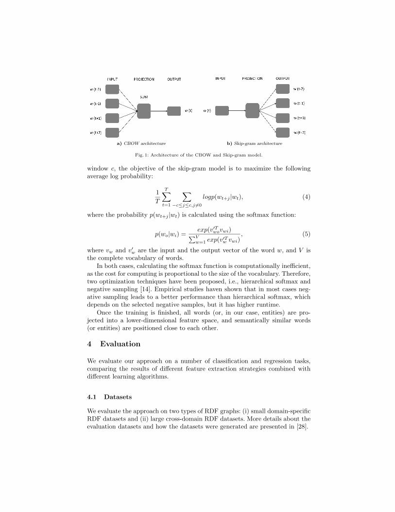
Continuous Bag-of-Words Model The CBOW model predicts target wordsfrom context words within a given window. The model architecture is shownin Fig. 1a. The input layer is comprised from all the surrounding words forwhich the input vectors are retrieved from the input weight matrix, averaged,and projected in the projection layer. Then, using the weights from the outputweight matrix, a score for each word in the vocabulary is computed, which isthe probability of the word being a target word. Formally, given a sequence oftraining words w1, w2, w3, ..., wT , and a context window c, the objective of theCBOW model is to maximize the average log probability:
1
T
T∑t=1
logp(wt|wt−c...wt+c), (1)
where the probability p(wt|wt−c...wt+c) is calculated using the softmax function:
p(wt|wt−c...wt+c) =exp(vT v′wt
)∑Vw=1 exp(vT v′w)
, (2)
where v′w is the output vector of the word w, V is the complete vocabulary ofwords, and v is the averaged input vector of all the context words:
v =1
2c
∑−c≤j≤c,j 6=0
vwt+j (3)
Skip-Gram Model The skip-gram model does the inverse of the CBOW modeland tries to predict the context words from the target words (Fig. 1b). Moreformally, given a sequence of training words w1, w2, w3, ..., wT , and a context
a) CBOW architecture b) Skip-gram architecture
Fig. 1: Architecture of the CBOW and Skip-gram model.
window c, the objective of the skip-gram model is to maximize the followingaverage log probability:
1
T
T∑t=1
∑−c≤j≤c,j 6=0
logp(wt+j |wt), (4)
where the probability p(wt+j |wt) is calculated using the softmax function:
p(wo|wi) =exp(v′Twovwi)∑Vw=1 exp(v′Tw vwi)
, (5)
where vw and v′w are the input and the output vector of the word w, and V isthe complete vocabulary of words.
In both cases, calculating the softmax function is computationally inefficient,as the cost for computing is proportional to the size of the vocabulary. Therefore,two optimization techniques have been proposed, i.e., hierarchical softmax andnegative sampling [14]. Empirical studies haven shown that in most cases neg-ative sampling leads to a better performance than hierarchical softmax, whichdepends on the selected negative samples, but it has higher runtime.
Once the training is finished, all words (or, in our case, entities) are pro-jected into a lower-dimensional feature space, and semantically similar words(or entities) are positioned close to each other.
4 Evaluation
We evaluate our approach on a number of classification and regression tasks,comparing the results of different feature extraction strategies combined withdifferent learning algorithms.
4.1 Datasets
We evaluate the approach on two types of RDF graphs: (i) small domain-specificRDF datasets and (ii) large cross-domain RDF datasets. More details about theevaluation datasets and how the datasets were generated are presented in [28].
Small RDF Datasets These datasets are derived from existing RDF datasets,where the value of a certain property is used as a classification target:
– The AIFB dataset describes the AIFB research institute in terms of its staff,research groups, and publications. In [1], the dataset was first used to predictthe affiliation (i.e., research group) for people in the dataset. The datasetcontains 178 members of five research groups, however, the smallest groupcontains only four people, which is removed from the dataset, leaving fourclasses.
– The MUTAG dataset is distributed as an example dataset for the DL-Learner toolkit2. It contains information about 340 complex molecules thatare potentially carcinogenic, which is given by the isMutagenic property.The molecules can be classified as “mutagenic” or “not mutagenic”.
– The BGS dataset was created by the British Geological Survey and describesgeological measurements in Great Britain3. It was used in [33] to predict thelithogenesis property of named rock units. The dataset contains 146 namedrock units with a lithogenesis, from which we use the two largest classes.
Large RDF Datasets As large cross-domain datasets we use DBpedia [11]and Wikidata [31].
We use the English version of the 2015-10 DBpedia dataset, which contains4, 641, 890 instances and 1, 369 mapping-based properties. In our evaluation weonly consider object properties, and ignore datatype properties and literals.
For the Wikidata dataset we use the simplified and derived RDF dumps from2016-03-284. The dataset contains 17, 340, 659 entities in total. As for the DBpe-dia dataset, we only consider object properties, and ignore the data propertiesand literals.
We use the entity embeddings on five different datasets from different do-mains, for the tasks of classification and regression. Those five datasets are usedto provide classification/regression targets for the large RDF datasets (see Ta-ble 1).
– The Cities dataset contains a list of cities and their quality of living, as cap-tured by Mercer5. We use the dataset both for regression and classification.
– The Metacritic Movies dataset is retrieved from Metacritic.com6, which con-tains an average rating of all time reviews for a list of movies [26]. The ini-tial dataset contained around 10, 000 movies, from which we selected 1, 000movies from the top of the list, and 1, 000 movies from the bottom of thelist. We use the dataset both for regression and classification.
– Similarly, the Metacritic Albums dataset is retrieved from Metacritic.com7,which contains an average rating of all time reviews for a list of albums [27].
Table 1: Datasets overview. For each dataset, we depict the number of instances, the machine learningtasks in which the dataset is used (C stands for classification, and R stands for regression) and thesource of the dataset.
Dataset #Instances ML Task Original Source
Cities 212 R/C (c=3) Mercer
Metacritic Albums 1600 R/C (c=2) Metacritic
Metacritic Movies 2000 R/C (c=2) Metacritic
AAUP 960 R/C (c=3) JSE
Forbes 1585 R/C (c=3) Forbes
AIFB 176 C (c=4) AIFB
MUTAG 340 C (c=2) MUTAG
BGS 146 C (c=2) BGS
– The AAUP (American Association of University Professors) dataset containsa list of universities, including eight target variables describing the salaryof different staff at the universities8. We use the average salary as a targetvariable both for regression and classification, discretizing the target variableinto “high”, “medium” and “low”, using equal frequency binning.
– The Forbes dataset contains a list of companies including several featuresof the companies, which was generated from the Forbes list of leading com-panies 20159. The target is to predict the company’s market value as a re-gression task. To use it for the task of classification we discretize the targetvariable into “high”, “medium”, and “low”, using equal frequency binning.
4.2 Experimental Setup
The first step of our approach is to convert the RDF graphs into a set of se-quences. For each of the small RDF datasets, we first build two corpora ofsequences, i.e., the set of sequences generated from graph walks with depth 8(marked as W2V), and set of sequences generated from Weisfeiler-Lehman sub-tree kernels (marked as K2V). For the Weisfeiler-Lehman algorithm, we use 4iterations and depth of 2, and after each iteration we extract all walks for eachentity with the same depth. We use the corpora of sequences to build bothCBOW and Skip-Gram models with the following parameters: window size = 5;number of iterations = 10; negative sampling for optimization; negative samples= 25; with average input vector for CBOW. We experiment with 200 and 500dimensions for the entities’ vectors. The remaining parameters have the defaultvalue as proposed in [14].
As the number of generated walks increases exponentially [34] with thegraph traversal depth, calculating Weisfeiler-Lehman subtrees RDF kernels, orall graph walks with a given depth d for all of the entities in the large RDF graphquickly becomes unmanageable. Therefore, to extract the entities embeddings forthe large RDF datasets, we use only random graph walks entity sequences. Moreprecisely, we follow the approach presented in [22] to generate limited numberof random walks for each entity. For DBpedia, we experiment with 500 walks
8 http://www.amstat.org/publications/jse/jse data archive.htm9 http://www.forbes.com/global2000/list/
per entity with depth of 4 and 8, while for Wikidata, we use only 200 walks perentity with depth of 4. Additionally, for each entity in DBpedia and Wikidata,we include all the walks of depth 2, i.e., direct outgoing relations. We use thecorpora of sequences to build both CBOW and Skip-Gram models with the fol-lowing parameters: window size = 5; number of iterations = 5; negative samplingfor optimization; negative samples = 25; with average input vector for CBOW.We experiment with 200 and 500 dimensions for the entities’ vectors. All themodels, as well as the code, are publicly available10.
We compare our approach to several baselines. For generating the data min-ing features, we use three strategies that take into account the direct relationsto other resources in the graph [20], and two strategies for features derived fromgraph sub-structures [34]:
– Features derived from specific relations. In the experiments we use the re-lations rdf:type (types), and dcterms:subject (categories) for datasets linkedto DBpedia.
– Features derived from generic relations, i.e., we generate a feature for eachincoming (rel in) or outgoing relation (rel out) of an entity, ignoring thevalue or target entity of the relation.
– Features derived from generic relations-values, i.e, we generate feature foreach incoming (rel-vals in) or outgoing relation (rel-vals out) of an entityincluding the value of the relation.
– Kernels that count substructures in the RDF graph around the instancenode. These substructures are explicitly generated and represented as sparsefeature vectors.• The Weisfeiler-Lehman (WL) graph kernel for RDF [34] counts full sub-
trees in the subgraph around the instance node. This kernel has two pa-rameters, the subgraph depth d and the number of iterations h (whichdetermines the depth of the subtrees). We use two pairs of settings,d = 1, h = 2 and d = 2, h = 3.
• The Intersection Tree Path kernel for RDF [34] counts the walks inthe subtree that spans from the instance node. Only the walks thatgo through the instance node are considered. We will therefore refer toit as the root Walk Count (WC) kernel. The root WC kernel has oneparameter: the length of the paths l, for which we test 2 and 3.
We perform two learning tasks, i.e., classification and regression. For classifi-cation tasks, we use Naive Bayes, k-Nearest Neighbors (k=3), C4.5 decision tree,and Support Vector Machines. For the SVM classifier we optimize the parame-ter C in the range {10−3, 10−2, 0.1, 1, 10, 102, 103}. For regression, we use LinearRegression, M5Rules, and k-Nearest Neighbors (k=3). We measure accuracy forclassification tasks, and root mean squared error (RMSE) for regression tasks.The results are calculated using stratfied 10-fold cross validation.
The strategies for creating propositional features from Linked Open Dataare implemented in the RapidMiner LOD extension11 [21, 23]. The experiments,
Table 2: Classification results on the small RDF datasets. The best results are marked in bold.Experiments marked with “\” did not finish within ten days, or have run out of memory.
including the feature generation and the evaluation, were performed using theRapidMiner data analytics platform.12 The RapidMiner processes and the com-plete results can be found online.13
4.3 Results
The results for the task of classification on the small RDF datasets are given inTable 2. From the results we can observe that the K2V approach outperformsall the other approaches. More precisely, using the skip-gram feature vectorsof size 500 in an SVM model provides the best results on all three datasets.The W2V approach on all three datasets performs closely to the standard graphsubstructure feature generation strategies, but it does not outperform them. K2Voutperforms W2V because it is able to capture more complex substructures inthe graph, like sub-trees, while W2V focuses only on graph paths.
The results for the task of classification on the five different datasets usingthe DBpedia and Wikidata entities’ vectors are given in Table 3, and the resultsfor the task of regression on the 5 different dataset using the DBpedia andWikidata entities’ vectors are given in Table 4. We can observe that the latentvectors extracted from DBpedia and Wikidata outperform all of the standardfeature generation approaches. In general, the DBpedia vectors work better thanthe Wikidata vectors, where the skip-gram vectors with size 200 or 500 built ongraph walks of depth 8 on most of the datasets lead to the best performances.An exception is the AAUP dataset, where the Wikidata skip-gram 500 vectorsoutperform the other approaches.
12 https://rapidminer.com/13 http://data.dws.informatik.uni-mannheim.de/rmlod/LOD ML Datasets/
a) DBpedia vectors b) Wikidata vectors
Fig. 2: Two-dimensional PCA projection of the 500-dimensional Skip-gram vectors of countries andtheir capital cities.
On both tasks, we can observe that the skip-gram vectors perform betterthan the CBOW vectors. Also, the vectors with higher dimensionality and pathswith bigger depth on most of the datasets lead to a better representation of theentities and better performances. However, for the variety of tasks at hand, thereis no universal approach, i.e., embedding model and a machine learning method,that consistently outperforms the others.
4.4 Semantics of Vector Representations
To analyze the semantics of the vector representations, we employ PrincipalComponent Analysis (PCA) to project the entities’ feature vectors into a twodimensional feature space. We selected seven countries and their capital cities,and visualized their vectors as shown in Figure 2. Figure 2a shows the corre-sponding DBpedia vectors, and Figure 2b shows the corresponding Wikidatavectors. The figure illustrates the ability of the model to automatically orga-nize entities of different types, and preserve the relationship between differententities. For example, we can see that there is a clear separation between thecountries and the cities, and the relation “capital” between each pair of countryand the corresponding capital city is preserved. Furthermore, we can observethat more similar entities are positioned closer to each other, e.g., we can seethat the countries that are part of the EU are closer to each other, and the sameapplies for the Asian countries.
4.5 Features Increase Rate
Finally, we conduct a scalability experiment, where we examine how the numberof instances affects the number of generated features by each feature generationstrategy. For this purpose we use the Metacritic Movies dataset. We start witha random sample of 100 instances, and in each next step we add 200 (or 300)
Table
3:
Cla
ssificatio
nre
sults.
The
first
num
ber
repre
sents
the
dim
ensio
nality
of
the
vecto
rs,w
hile
the
second
num
ber
repre
sent
the
valu
efo
rth
edepth
para
mete
r.T
he
best
resu
ltsare
mark
ed
inb
old
.E
xp
erim
ents
mark
ed
with
“\”
did
not
finish
with
inte
ndays,
or
have
run
out
of
mem
ory
.
Stra
tegy/D
ata
setC
itiesM
etacritic
Mov
iesM
etacritic
Alb
um
sA
AU
PF
orb
es
NB
KN
NSV
MC
4.5
NB
KN
NSV
MC
4.5
NB
KN
NSV
MC
4.5
NB
KN
NSV
MC
4.5
NB
KN
NSV
MC
4.5
typ
es55.7
156.1
763.2
159.0
568.0
057.6
071.4
070.0
066.5
050.7
562.3
154.4
441.0
085.6
291.6
792.7
855.0
875.8
475.6
775.8
5
categ
ories
55.7
449.9
862.3
956.1
775.2
562.7
076.3
569.5
067.4
054.1
364.5
056.6
248.0
085.8
390.7
891.8
760.3
876.1
175.7
075.7
0
relin
60.4
158.4
671.7
060.3
552.7
549.9
060.3
560.1
051.1
362.1
965.2
560.7
545.6
385.9
490.6
292.8
150.2
476.4
975.1
676.1
0
relout
47.6
260.0
066.0
456.7
152.9
058.4
566.4
062.7
058.7
563.7
562.2
564.5
041.1
585.8
389.5
891.3
564.7
375.8
475.7
375.9
2
relin
&out
59.4
458.5
766.0
456.4
752.9
559.3
067.7
562.5
558.6
964.5
067.3
861.5
642.7
185.9
489.6
792.5
022.2
775.9
676.3
475.9
8
rel-vals
in\
\\
\50.6
050.0
050.6
050.0
050.8
850.0
050.8
150.0
054.0
684.6
989.5
1\
14.9
576.1
576.9
775.7
3
rel-vals
out
53.7
935.9
155.6
664.1
378.5
054.7
878.7
1\
74.0
652.5
676.9
9\
57.8
185.7
391.4
691.7
867.0
975.6
175.7
476.7
4
rel-vals
in&
out
\\
\\
77.9
055.7
577.8
2\
74.2
551.2
575.8
5\
63.4
484.6
991.5
6\
67.2
075.8
875.9
676.7
5
WL
12
70.9
849.3
165.3
475.2
975.4
566.9
079.3
070.8
073.6
364.6
976.2
562.0
058.3
391.0
491.4
692.4
064.1
775.7
175.1
076.5
9
WL
23
65.4
853.2
969.9
069.3
1\
\\
\\
\\
\\
\\
\\
\\
\W
C2
72.7
147.3
966.4
875.1
375.3
965.8
974.9
369.0
872.0
060.6
376.8
863.6
957.2
990.6
393.4
492.6
064.2
375.7
776.2
276.4
7
WC
365.5
252.3
667.9
565.1
574.2
555.3
078.4
0\
72.8
152.8
777.9
4\
57.1
990.7
390.9
492.6
064.0
475.6
576.2
276.5
9
DB
2vec
CB
OW
200
459.3
268.8
477.3
964.3
265.6
079.7
482.9
074.3
370.7
271.8
676.3
667.2
473.3
689.6
529.0
092.4
589.3
880.9
476.8
384.8
1
DB
2vec
CB
OW
500
459.3
271.3
476.3
766.3
465.6
579.4
982.7
573.8
769.7
171.9
375.4
165.6
572.7
189.6
529.1
192.0
189.0
280.8
276.9
585.1
7
DB
2vec
SG
200
460.3
471.8
276.3
765.3
765.2
580.4
483.2
573.8
768.9
573.8
976.1
167.8
771.2
089.6
528.9
092.1
288.7
880.8
277.9
285.7
7
DB
2vec
SG
500
458.3
472.8
476.8
767.8
465.4
580.1
483.65
72.8
270.4
174.3
478.4
467.4
971.1
989.6
528.9
092.2
388.3
080.9
477.2
584.8
1
DB
2vec
CB
OW
200
869.2
669.8
767.3
263.1
357.8
370.0
865.2
567.4
767.9
164.4
472.4
265.3
968.1
885.3
328.9
090.5
077.3
580.3
428.9
085.1
7
DB
2vec
CB
OW
500
862.2
669.8
776.8
463.2
158.7
869.8
269.4
667.6
767.5
365.8
374.2
663.4
262.9
085.2
229.1
190.6
189.8
680.3
478.6
584.8
1
DB
2vec
SG
200
873.3
275.8
978.9
260.7
479.9
479.4
983.3
075.1
377.2
576.8
779.72
69.1
478.5
385.1
229.2
291.0
490.10
80.5
878.9
684.6
8
DB
2vec
SG
500
889.73
69.1
684.1
972.2
580.2
478.6
882.8
072.4
273.5
776.3
078.2
068.7
075.0
794.48
29.1
194.1
588.5
380.5
877.7
986.3
8
WD
2vec
CB
OW
200
468.7
657.7
175.5
661.3
751.4
952.2
051.6
449.0
150.8
650.2
951.4
450.0
950.5
490.1
889.6
388.8
349.8
481.0
876.7
779.1
4
WD
2vec
CB
OW
500
468.2
457.7
585.5
664.5
449.2
248.5
651.0
450.9
853.0
850.0
352.3
353.2
848.4
590.3
989.7
488.3
151.9
580.7
478.1
880.3
2
WD
2vec
SG
200
472.5
857.5
375.4
852.3
269.5
370.1
475.3
967.0
060.3
262.0
364.7
658.5
460.8
790.5
089.6
389.9
865.4
581.1
777.7
477.0
3
WD
2vec
SG
500
483.2
060.7
279.8
761.6
771.1
070.1
976.3
067.3
155.3
158.9
263.4
256.6
355.8
590.6
089.6
387.6
958.9
581.1
779.0
079.5
6
Table
4:R
egre
ssio
nre
sult
s.T
he
firs
tnum
ber
repre
sents
the
dim
ensi
onality
of
the
vecto
rs,w
hile
the
second
num
ber
repre
sent
the
valu
efo
rth
edepth
para
mete
r.T
he
best
resu
lts
are
mark
ed
inb
old
.E
xp
eri
ments
that
did
not
finis
hw
ithin
ten
days,
or
that
have
run
out
of
mem
ory
are
mark
ed
wit
h“\”
.
Str
ate
gy/D
ata
set
Cit
ies
Met
acr
itic
Mov
ies
Met
acr
itic
Alb
um
sA
AU
PF
orb
es
LR
KN
NM
5L
RK
NN
M5
LR
KN
NM
5L
RK
NN
M5
LR
KN
NM
5
typ
es24.3
022.1
618.7
977.8
030.6
822.1
616.4
518.3
613.9
59.8
334.9
56.2
829.2
221.0
718.3
2
cate
gori
es18.8
822.6
822.3
284.5
723.8
722.5
016.7
316.6
413.9
58.0
834.9
46.1
619.1
621.4
818.3
9
rel
in49.8
718.5
319.2
122.6
041.4
022.5
613.5
022.0
613.4
39.6
934.9
86.5
627.5
620.9
318.6
0
rel
out
49.8
718.5
319.2
121.4
524.4
220.7
413.3
214.5
913.0
68.8
234.9
56.3
221.7
321.1
118.9
7
rel
in&
out
40.8
018.2
118.8
021.4
524.4
220.7
413.3
314.5
212.9
112.9
734.9
56.3
626.4
420.9
819.5
4
rel-
vals
in\
\\
21.4
624.1
920.4
313.9
423.0
513.9
5\
34.9
66.2
7\
20.8
619.3
1
rel-
vals
out
20.9
323.8
720.9
725.9
932.1
822.9
3\
15.2
813.3
4\
34.9
56.1
8\
20.4
818.3
7
rel-
vals
in&
out
\\
\\
25.3
720.9
6\
15.4
713.3
3\
34.9
46.1
8\
20.2
018.2
0
WL
12
20.2
124.6
020.8
5\
21.6
219.8
4\
13.9
912.8
1\
34.9
66.2
7\
19.8
119.4
9W
L2
317.7
920.4
217.0
4\
\\
\\
\\
\\
\\
\W
C2
20.3
325.9
519.5
5\
22.8
022.9
9\
14.5
412.8
79.1
234.9
56.2
4\
20.4
519.2
6
WC
319.5
133.1
619.0
5\
23.8
619.1
9\
19.5
113.0
2\
35.3
96.3
1\
20.5
819.0
4
DB
2vec
CB
OW
200
414.3
712.5
514.3
315.9
017.4
615.8
911.7
912.4
511.5
912.1
345.7
612.0
018.3
226.1
917.4
3
DB
2vec
CB
OW
500
414.9
912.4
614.6
615.9
017.4
515.7
311.4
912.6
011.4
812.4
445.6
712.3
018.2
326.2
717.6
2
DB
2vec
SG
200
413.3
812.5
415.1
315.8
117.0
715.8
411.3
012.3
611.4
212.1
345.7
212.1
017.6
326.1
317.8
5
DB
2vec
SG
500
414.7
313.2
516.8
015.6
617.1
415.6
711.2
012.1
111.2
812.0
945.7
611.9
318.2
326.0
917.7
4
DB
2vec
CB
OW
200
816.1
717.1
417.5
621.5
523.7
521.4
613.3
515.4
113.4
36.4
755.7
66.4
724.1
726.4
822.6
1
DB
2vec
CB
OW
500
818.1
317.1
918.5
020.7
723.6
720.6
913.2
015.1
413.2
56.5
455.3
36.5
521.1
625.9
020.3
3
DB
2vec
SG
200
812.8
514.9
512.9
215.1
517.1
315.12
10.9
011.4
310.9
06.2
256.9
56.2
518.6
621.2
018.5
7
DB
2vec
SG
500
811.9
212.6
710.19
15.4
517.8
015.5
010.89
11.7
210.9
76.2
656.9
56.2
918.3
521.0
416.61
WD
2vec
CB
OW
200
420.1
517.5
220.0
223.5
425.9
023.3
914.7
316.1
214.5
516.8
042.6
16.6
027.4
822.6
021.7
7
WD
2vec
CB
OW
500
423.7
618.3
320.3
924.1
422.1
824.5
614.0
916.0
914.0
013.0
842.8
96.0
850.2
321.9
226.6
6
WD
2vec
SG
200
420.4
718.6
920.7
219.7
221.4
419.1
013.5
113.9
113.6
76.8
642.8
26.5
223.6
921.5
920.4
9
WD
2vec
SG
500
422.2
519.4
119.2
325.9
921.2
619.1
913.2
314.9
613.2
58.2
742.8
46.05
21.9
821.7
321.5
8
Fig. 3: Features increase rate per strategy (log scale).
unused instances, until the complete dataset is used, i.e., 2, 000 instances. Thenumber of generated features for each sub-sample of the dataset using each ofthe feature generation strategies is shown in Figure 3.
From the chart, we can observe that the number of generated features sharplyincreases when adding more samples in the datasets, especially for the strategiesbased on graph substructures. However, the number of features remains the samewhen using the RDF2Vec approach, independently of the number of samples inthe data. Thus, by design, it scales to larger datasets without increasing thedimensionality of the dataset.
5 Conclusion
In this paper, we have presented RDF2Vec, an approach for learning latent nu-merical representations of entities in RDF graphs. In this approach, we firstconvert the RDF graphs in a set of sequences using two strategies, Weisfeiler-Lehman Subtree RDF Graph Kernels and graph walks, which are then used tobuild neural language models. The evaluation shows that such entity represen-tations could be used in two different machine learning tasks, outperformingstandard feature generation approaches.
So far we have considered only simple machine learning tasks, i.e, classifi-cation and regression, but in the future work we would extend the number ofapplications. For example, the latent representation of the entities could be usedfor building content-based recommender systems [4]. The approach could also beused for link predictions, type prediction, graph completion and error detectionin knowledge graphs [19], as shown in [15, 17]. Furthermore, we could use thisapproach for the task of measuring semantic relatedness between two entities,which is the basis for numerous tasks in information retrieval, natural languageprocessing, and Web-based knowledge extractions [6]. To do so, we could easilycalculate the relatedness between two entities as the probability of one entitybeing the context of the other entity, using the softmax function given in Equa-tion 2 and 5, using the input and output weight matrix of the neural model.
Similarly, the approach can be extended for entity summarization, which is alsoan important task when consuming and visualizing large quantities of data [2].
Acknowledgements The work presented in this paper has been partly fundedby the German Research Foundation (DFG) under grant number PA 2373/1-1(Mine@LOD).
References
1. Bloehdorn, S., Sure, Y.: Kernel methods for mining instance data in ontologies. In:Proceedings of the 6th International The Semantic Web and 2Nd Asian Conferenceon Asian Semantic Web Conference. pp. 58–71. ISWC’07/ASWC’07 (2007)
2. Cheng, G., Tran, T., Qu, Y.: Relin: relatedness and informativeness-based central-ity for entity summarization. In: The Semantic Web–ISWC, pp. 114–129 (2011)
3. Cheng, W., Kasneci, G., Graepel, T., Stern, D., Herbrich, R.: Automated featuregeneration from structured knowledge. In: CIKM (2011)
4. Di Noia, T., Ostuni, V.C.: Recommender systems and linked open data. In: Rea-soning Web. Web Logic Rules, pp. 88–113. Springer (2015)
5. Fanizzi, N., d’Amato, C.: A declarative kernel for alc concept descriptions. In:Foundations of Intelligent Systems, pp. 322–331 (2006)
6. Hoffart, J., Seufert, S., Nguyen, D.B., Theobald, M., Weikum, G.: Kore: keyphraseoverlap relatedness for entity disambiguation. In: Proceedings of the 21st ACMinternational conference on Information and knowledge management. pp. 545–554.ACM (2012)
7. Huang, Y., Tresp, V., Nickel, M., Kriegel, H.P.: A scalable approach for statisticallearning in semantic graphs. Semantic Web (2014)
8. Kappara, V.N.P., Ichise, R., Vyas, O.: Liddm: A data mining system for linkeddata. In: LDOW (2011)
9. Khan, M.A., Grimnes, G.A., Dengel, A.: Two pre-processing operators for im-proved learning from semanticweb data. In: RCOMM (2010)
10. Kramer, S., Lavrac, N., Flach, P.: Propositionalization approaches to relationaldata mining. In: Dzeroski, S., Lavrac, N. (eds.) Relational Data Mining, pp. 262–291. Springer Berlin Heidelberg (2001)
11. Lehmann, J., Isele, R., Jakob, M., Jentzsch, A., Kontokostas, D., Mendes, P.N.,Hellmann, S., Morsey, M., van Kleef, P., Auer, S., Bizer, C.: DBpedia – A Large-scale, Multilingual Knowledge Base Extracted from Wikipedia. Semantic WebJournal (2013)
12. Losch, U., Bloehdorn, S., Rettinger, A.: Graph kernels for rdf data. In: The Se-mantic Web: Research and Applications, pp. 134–148. Springer (2012)
13. Mikolov, T., Chen, K., Corrado, G., Dean, J.: Efficient estimation of word repre-sentations in vector space. arXiv preprint arXiv:1301.3781 (2013)
14. Mikolov, T., Sutskever, I., Chen, K., Corrado, G.S., Dean, J.: Distributed repre-sentations of words and phrases and their compositionality. In: Advances in neuralinformation processing systems. pp. 3111–3119 (2013)
15. Minervini, P., Fanizzi, N., d’Amato, C., Esposito, F.: Scalable learning of entityand predicate embeddings for knowledge graph completion. In: 2015 IEEE 14thInternational Conference on Machine Learning and Applications (ICMLA). pp.162–167. IEEE (2015)
16. Mynarz, J., Svatek, V.: Towards a benchmark for LOD-enhanced knowledge dis-covery from structured data. In: The Second International Workshop on KnowledgeDiscovery and Data Mining Meets Linked Open Data (2013)
17. Nickel, M., Murphy, K., Tresp, V., Gabrilovich, E.: A review of relational machinelearning for knowledge graphs: From multi-relational link prediction to automatedknowledge graph construction. arXiv preprint arXiv:1503.00759 (2015)
18. Paulheim, H.: Exploiting linked open data as background knowledge in data min-ing. In: Workshop on Data Mining on Linked Open Data (2013)
19. Paulheim, H.: Knowlegde Graph Refinement: A Survey of Approaches and Evalu-ation Methods. Semantic Web Journal (2016), to appear
20. Paulheim, H., Fumkranz, J.: Unsupervised generation of data mining features fromlinked open data. In: Proceedings of the 2nd international conference on web in-telligence, mining and semantics. p. 31. ACM (2012)
21. Paulheim, H., Ristoski, P., Mitichkin, E., Bizer, C.: Data mining with backgroundknowledge from the web. RapidMiner World (2014)
22. Perozzi, B., Al-Rfou, R., Skiena, S.: Deepwalk: Online learning of social represen-tations. In: Proceedings of the 20th ACM SIGKDD international conference onKnowledge discovery and data mining. pp. 701–710. ACM (2014)
23. Ristoski, P., Bizer, C., Paulheim, H.: Mining the web of linked data with rapid-miner. Web Semantics: Science, Services and Agents on the World Wide Web 35,142–151 (2015)
24. Ristoski, P., Paulheim, H.: A comparison of propositionalization strategies for cre-ating features from linked open data. In: Linked Data for Knowledge Discovery(2014)
25. Ristoski, P., Paulheim, H.: Semantic web in data mining and knowledge discov-ery: A comprehensive survey. Web Semantics: Science, Services and Agents on theWorld Wide Web (2016)
26. Ristoski, P., Paulheim, H., Svatek, V., Zeman, V.: The linked data mining challenge2015. In: KNOW@LOD (2015)
27. Ristoski, P., Paulheim, H., Svatek, V., Zeman, V.: The linked data mining challenge2016. In: KNOWLOD (2016)
28. Ristoski, P., de Vries, G.K.D., Paulheim, H.: A collection of benchmark datasets forsystematic evaluations of machine learning on the semantic web. In: InternationalSemantic Web Conference (To Appear). Springer (2016)
29. Schmachtenberg, M., Bizer, C., Paulheim, H.: Adoption of the linked data bestpractices in different topical domains. In: The Semantic Web–ISWC (2014)
30. Shervashidze, N., Schweitzer, P., Van Leeuwen, E.J., Mehlhorn, K., Borgwardt,K.M.: Weisfeiler-lehman graph kernels. The Journal of Machine Learning Research12, 2539–2561 (2011)
31. Vrandecic, D., Krotzsch, M.: Wikidata: a free collaborative knowledgebase. Com-munications of the ACM 57(10), 78–85 (2014)
32. de Vries, G.K.D.: A fast approximation of the Weisfeiler-Lehman graph kernel forRDF data. In: ECML/PKDD (1) (2013)
33. de Vries, G.K.D., de Rooij, S.: A fast and simple graph kernel for rdf. In: DMLOD(2013)
34. de Vries, G.K.D., de Rooij, S.: Substructure counting graph kernels for machinelearning from rdf data. Web Semantics: Science, Services and Agents on the WorldWide Web 35, 71–84 (2015)
35. Yanardag, P., Vishwanathan, S.: Deep graph kernels. In: Proceedings of the 21thACM SIGKDD International Conference on Knowledge Discovery and Data Min-ing. pp. 1365–1374. ACM (2015)