Reaction Dynamics – Molecular Spectroscopy

Andrew Orr-Ewing

School of Chemistry

University of Bristol, UK

www.bristoldynamics.com

Outline

1. Requirements of spectroscopic probes for reaction dynamics

2. Fundamentals of molecular spectroscopy

3. Spectroscopic techniques for reaction dynamics

• Gas phase

• Condensed phase

4. Two-dimensional spectroscopy

5. Simulation of spectra using PGOPHER

1.0 Requirements of spectroscopic probes of reaction

dynamics

• High sensitivity – because of low densities in molecular beam experiments

• Specificity – to isolate signals from the molecules of interest

• Quantum-state resolution – for stringent tests of theory

• High time resolution – nanosecond to femtosecond to observe dynamics

Further desirable characteristics include measurement of correlated properties:

• Angular momentum polarization (alignment and orientation)

• Relative velocities and scattering angles, and dependence on quantum state

• Coherence and phase of quantum states, and dephasing times

1.1 Summary of spectroscopic techniques used in reaction dynamics

A. Gas phase / molecular beam experiments

• IR chemiluminescence

• Absorption spectroscopy (including Frequency Modulation Spectroscopy)

• Laser Induced Fluorescence

• REMPI and VUV ionization (combined with velocity map imaging, VMI)

• Photoelectron spectroscopy – Katharine Reid’s lecture

• Transient absorption spectroscopy

• XUV and X-ray absorption spectroscopy

• Attosecond spectroscopy with HHG pulses – Valerie Blanchet’s lecture

B. Condensed phase experiments

• Transient absorption spectroscopy

• Femtosecond stimulated Raman Spectroscopy

• 2D IR and 2D electronic spectroscopy

• Time-resolved photoelectron spectroscopy with liquid jets

2.0 Fundamentals of molecular spectroscopy

The spectroscopic methods probe rotational, vibrational and

electronic energy levels (and parities) of molecules.

The patterns of these energy levels and the high-resolution

spectroscopy of small molecules are discussed in numerous

textbooks:

e.g. P.F. Bernath, Spectra of Atoms and Molecules

Focus here on:

• Transition dipole moments for molecules and symmetry constraints

• Multi-photon transitions and selection rules

• Spectroscopy of molecular ensembles: the density matrix picture for pump-

probe and 2D spectroscopy

ℎ 𝑡 = − 𝜇 ∙ 𝐸 𝑡 = − 𝜇 ∙ 𝐸0𝑐𝑜𝑠𝜔𝑡

1

01 𝜇 ∙ 𝐸 𝑡 0 ≠ 0

𝜎 𝜔 =𝜋

ℏ휀0𝑐𝜔10𝛿 𝜔10 − 𝜔 1 𝜇 ∙ 𝐸0 0

2

ℏ𝜔10

𝜎 𝜔 ∝ 1 𝜇 ∙ 𝐸0 02∝ 1 𝜇 0 ∙ 𝐸0

2∝ 𝜇10 ∙ 𝐸0

2

2.1 Transition dipole moments and absorption cross sections

The interaction of electromagnetic radiation with a molecule is treated using

perturbation theory.

The electric-dipole interaction of the molecule with light is:

With 𝜇 denoting the electric dipole moment operator, and the frequency of the

light.

The electric-dipole interaction can couple two states if

The absorption cross section () is a measure of the strength of the transition

and can be determined from the Beer-Lambert law:

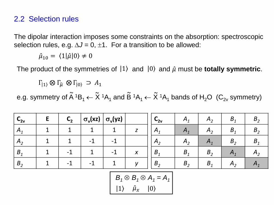
2.2 Selection rules

The dipolar interaction imposes some constraints on the absorption: spectroscopic

selection rules, e.g. J = 0, 1. For a transition to be allowed:

𝜇10 = 1 𝜇 0 ≠ 0

The product of the symmetries of and and 𝜇 must be totally symmetric. 1 0

Γ 1 ⨂ Γ 𝜇 ⨂Γ 0 ⊃ 𝐴1

e.g. symmetry of A 1B1 X 1A1 and B 1A1 X 1A1 bands of H2O (C2v symmetry)

C2v E C2 v(xz) v(yz)

A1 1 1 1 1 z

A2 1 1 -1 -1

B1 1 -1 1 -1 x

B2 1 -1 -1 1 y

C2v A1 A2 B1 B2

A1 A1 A2 B1 B2

A2 A2 A1 B2 B1

B1 B1 B2 A1 A2

B2 B2 B1 A2 A1

B1 B1 A1 = A1

1 0 𝜇𝑥

~ ~ ~~

2.3 Multiphoton transitions and selection rules

It is convenient to express the transition operator in spherical tensor form:

𝑇𝑞𝑘 𝜇

Electric dipole transition: 𝑘 = 1, 𝑞 = −1, 0, 1

Two-photon transition: 𝑘 = 2, 𝑞 = −2,−1, 0, 1, 2 and 𝑘 = 0, 𝑞 = 0

For rotational wavefunctions 𝐽𝐾𝑀 and with 𝜂 denoting electronic and

vibrational quantum numbers and states, the transition moments are:

𝜂′𝐽′𝐾′𝑀′ 𝑇𝑞𝑘 𝜇 𝜂𝐽𝐾𝑀 = (−1)𝐽

′−𝑀′ 𝐽′ 𝑘 𝐽

−𝑀′ 𝑞 𝑀×

𝑝(−1)𝐽′−𝐾′

(2𝐽′ + 1)(2𝐽 + 1)𝐽′ 𝑘 𝐽

−𝐾′ 𝑝 𝐾𝜂′ 𝑇𝑝

𝑘(𝜇) 𝜂

𝑘 is the rank of the tensor

𝑞 is the component (a projection quantum number with 𝑞 ≤ 𝑘)

𝐾 is the body-fixed projection of 𝐽. Use in a diatomic molecule.

𝑀 is the space-fixed projection of 𝐽.

The Wigner 3-j symbols impose selection rules (in the body-fixed frame):

𝐽′ 𝑘 𝐽

−𝐾′ 𝑝 𝐾= 0 unless −𝐾′ + 𝑝 + 𝐾 = 0

𝑝 = 𝐾′ − 𝐾 = Δ𝐾, or 𝑝 = Ω′ − Ω = ΔΩ for diatomic molecules.

e.g. The 𝐹 1Δ2 − 𝑋 1Σ0+ transition of HCl is allowed in a two-photon transition

with a transition dipole moment operator 𝑇22 𝜇 .

𝐹 1Δ2

𝑋 1Σ0+

PGOPHER: A program for simulating rotational,

vibrational and electronic spectra,

C.M. Western, J. Quant. Spectros. Radiat. Trans.

186, 221 (2017). http://pgopher.chm.bris.ac.uk/

v=2v=1v=0

v’=2v’=1v’=0 The PGOPHER simulation of the 2-photon

transition uses matrix

elements:

𝐹 1Δ2 𝑣′ = 0,1,2 𝑇22 𝜇 𝑋 1Σ0

+ 𝑣 = 0,1,2

𝐹 1Δ2 − 𝑋 1Σ0+

For more detail on multiphoton selection rules see Ashfold et al. J. Chem. Soc.

Faraday Trans. 89, 1153 (1993)

Simulation of two-photon HCl spectrum using PGOPHER

𝐹 1Δ2 𝑣′ = 0 − 𝑋 1Σ0+ 𝑣 = 0

𝑓 3Δ2 𝑣′ = 0 − 𝑋 1Σ0+ 𝑣 = 0

HCl two-photon absorption spectrum

T = 200 K

R and S branches

Q branch

P and O branches

Q branch

R and S branches

P and O branches

J = +2 J = +1 J = 0 J = -1 J = -2

S branch R branch Q branch P branch O branch

Two-photon wavenumber / cm-1

3.0 Spectroscopic techniques for reaction dynamics

3.1 Laser induced fluorescence (LIF) spectroscopy

Excite a one-photon transition in a molecule

or radical (usually with nsec laser).

Image the fluorescence from an excited

electronic state.

Common applications in chemical dynamics

studies include detection of OH, e.g. in

reactions of O(3P) at liquid hydrocarbon

surfaces (K.G. McKendrick and coworkers).

Squalane

LIF excitation

v=0

v′=1

v′=0

30

8 n

m

A2+

X2

Collect fluorescence from A2+ state

3.2 Resonance Enhanced Multi-Photon Ionization (REMPI) spectroscopy

Use a focused, nanosecond laser pulse

from a dye laser or OPO to excite an n

photon absorption to a Rydberg state

followed by an m photon absorption

above the ionization limit.

(n + m) REMPI spectroscopy.

Detect the resulting cations in a TOF

mass spectrometer, often partnered with

velocity map imaging.

Convenient and popular (2+1) REMPI

schemes for detection of H, Cl, Br, H2,

HCl, HBr, CH3, NH3, etc.

e.g. application in study of Cl + CH4

HCl + CH3 reaction (R.N. Zare, K. Liu, F.F.

Crim, …)

AB

AB*

AB+

(2+1) REMPI

scheme

g3-X1+

F1-X1+

Cl + CH3CH2OH HCl + CH2CH2OH

Two-photon wavenumber / cm-1

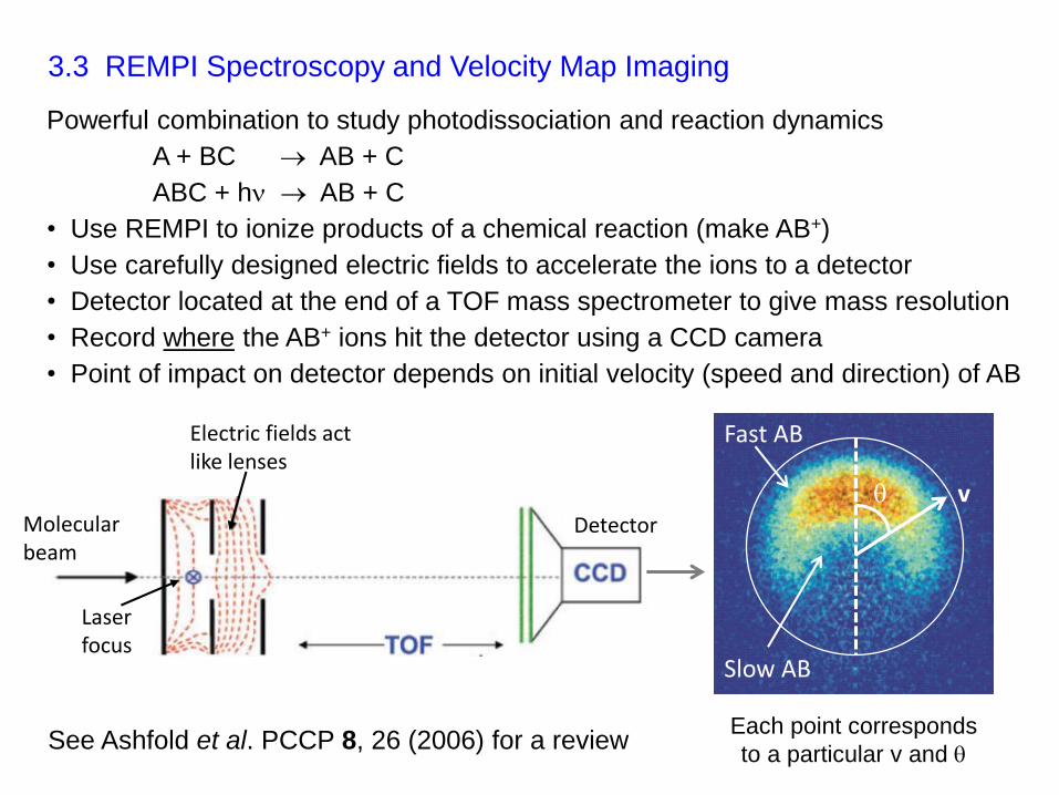
3.3 REMPI Spectroscopy and Velocity Map Imaging

See Ashfold et al. PCCP 8, 26 (2006) for a review

Electric fields act like lenses

Molecular beam

Detector

Laser focus

v

Each point corresponds

to a particular v and

Fast AB

Slow AB

Powerful combination to study photodissociation and reaction dynamics

A + BC AB + C

ABC + h AB + C

• Use REMPI to ionize products of a chemical reaction (make AB+)

• Use carefully designed electric fields to accelerate the ions to a detector

• Detector located at the end of a TOF mass spectrometer to give mass resolution

• Record where the AB+ ions hit the detector using a CCD camera

• Point of impact on detector depends on initial velocity (speed and direction) of AB

Lin et al., Science 300, 966 (2003)

F

CD4

00 21

2223

Example: VMI of F + CD4 DF(v) + CD3

• REMPI detection of CD3 in umbrella modes v2 = 0, 1, 2, 3 (denoted 20, 21, 22, 23).

• Select quantum state of CD3 by choice of laser wavelength for REMPI

• By energy conservation, slower CD3 greater internal (vibrational) energy of DF

DF

DF DF

3.4 Photoelectron spectroscopy as a probe of chemical dynamics

Time-resolved photoelectron spectroscopy Anion photodetachment

Stolow et al. Chem Rev. 104, 1719 (2004)

Suzuki, Ann. Rev. Phys. Chem. 57, 555 (2006)

tSn

Tn

UV

AB

AB+ + e-

ABC-

A+BC AB+C

e.g., Kim et al., Science 349, 510 (2015)

e- KE

ABCǂ

Example: Anion photodetachment study of the F + H2 reaction

J.B. Kim et al., Science 349, 510 (2015)

Simulation

Simulation

convoluted with

3 meV Gaussian

Experiment

𝑃 𝐸 = 𝜓𝑣𝑖𝑏 𝐹𝐻2− 𝜓𝑠𝑐𝑎𝑡

𝐸 𝐹𝐻2

Simulated spectra are computed using Franck-Condon factors

(assuming a constant electronic transition dipole matrix

element):

3.5 Transient absorption spectroscopy

CII 100Beer-Lambert Law:

CI

IA 0

10log

/ cm-1

I

UV pulse off

UV pulse on

ΔA

0

+

-

Transient

absorption

Bleaches

ΔA(t) = -logIpump on

Ipump off

/ cm-1

BrCN PE curves

Br + CN

Br* + CN

220 n

m

80 70 60 50 40 30 20

R Branch (N)

1 20

80 70 60 30P Branch (N)

Wavelength (nm)

Time (fs)

Ab

sorb

an

ce (

mO

D)

376 378 380 382 384 386 388 390 392

2

4

8

12 15 120 225 400-150

0

6

14

10

Wavelength (nm)

Ab

so

rba

nce

(

mO

D)

CN B2+ X2+

Example: Transient absorption

spectroscopy of CN radicals

from 220-nm photolysis of BrCN

M.P. Grubb et al.,

Nat. Chem. 8, 1042 (2016)

Data analysis software available

at www.bristoldynamics.com

CN radicals are produced highly

rotationally excited (N ~ 50)

because of angular anisotropy on

the dissociative excited state PESs.

Attar et al. JPCLett 6, 5072 (2015)

Bhattacherjee et al., J. Chem. Phys. 144, 124311 (2016)

3.6 Transient XUV absorption spectroscopy: CH3I photodissociation

• UV photolysis pulse at 266 nm: n(I) *(C-I) excitation to 3Q0 and 1Q1 states

• 35-fs XUV probe pulse (by HHG): 4d core-to-valence excitation on Iodine atom

• Transient absorption spectroscopy (measure OD).

Attar et al. JPCLett 6, 5072 (2015)

CH3I photodissociation: observation

of dissociating intermediates on the 3Q0

and 1Q1 states.

Intermediates rise in ~40 fs and decay

by 90 fs as bond breaking is complete.

Core excitation gives atom / element

specific detection.

v=0

A

S

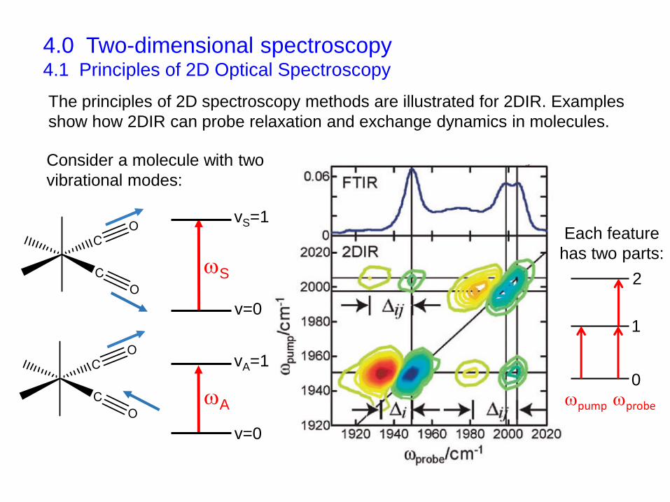
4.0 Two-dimensional spectroscopy4.1 Principles of 2D Optical Spectroscopy

vS=1

v=0

vA=1

1

0

2

pump probe

Each feature

has two parts:

The principles of 2D spectroscopy methods are illustrated for 2DIR. Examples

show how 2DIR can probe relaxation and exchange dynamics in molecules.

Consider a molecule with two

vibrational modes:

What is the effect of a laser pulse on a two-level system? We will develop a

2DIR response function treatment for an ensemble of molecules.

The dipolar interaction of the laser field with a molecule is

ℎ 𝑡 = − 𝜇 ∙ 𝐸 𝑡 = − 𝜇 ∙ 𝐸0𝑐𝑜𝑠𝜔𝑡

After the laser pulse, the molecule is in a linear combination of eigenstates:

𝜓 𝑡 = 𝑐0𝑒−𝑖𝐸0𝑡/ℏ 0 + 𝑐1𝑒

−𝑖𝐸1𝑡/ℏ 1

The cn coefficients contain the transition dipole moments, but are time-

independent because the laser pulse is now off.

The coherent superposition 𝜓 𝑡 corresponds to a wavepacket. An ensemble

of molecules cannot be described by a single wavefunction. Instead, the time-

dependence of this ensemble is called the molecular response, R(t).

1

0

ℏ𝜔10

4.2 Density matrix formalism for spectroscopy of molecular systems

In an ensemble of molecules we create a macroscopic polarization P(t)

because the molecules are all driven by the same laser pulse and are

initially oscillating in phase.

P(t) is obtained from the molecular response function by convoluting with

the electric field of the laser pulse(s).

𝑃 𝑡 = 0∞

𝑑𝑡1𝐸 𝑡 − 𝑡1 𝑅 𝑡1

For an ultrafast pulse, we can make the approximation P(t) R(t).

For one molecule the response is the expectation value of the transition

dipole operator:

𝑅 𝑡 = 𝜇 = 𝜓 𝑡 𝜇 𝜓 𝑡 ∝ 𝜇102 𝑠𝑖𝑛 𝜔10𝑡

The resulting polarization oscillates and emits radiation at 𝜔10 with a 90o

phase shift. A Fourier transform of the emitted time-dependent field gives the absorption spectrum.

In an ensemble of molecules in different environments, the frequencies of

oscillation differ. The oscillations lose their phase relationship and the

macroscopic polarization decays to zero over time. In the signal, we observe a

Free Induction Decay (FID).

For an ensemble we use a density matrix rather than a wavefunction description.

𝜌 =𝜌00 𝜌01

𝜌10 𝜌11=

𝑐0𝑐0∗ −𝑐0𝑐1

∗𝑒𝑖𝜔10𝑡

𝑐1𝑐0∗𝑒−𝑖𝜔10𝑡 𝑐1𝑐1

∗

Population relaxation and dephasing (e.g. by environmental fluctuations changing

the frequencies and hence phases of the individual wavefunctions) contribute

time-dependence to the cn coefficients.

Diagonal elements 𝜌00 and 𝜌11 describe the populations of the states 0 and 1 .

Non-zero off-diagonal elements 𝜌10 and 𝜌01describe coherences.

The coherences decay with dephasing time T2, e.g. 𝜌10 𝑡 = 𝜌10 𝑡 = 0 𝑒−𝑡/𝑇2

The excited population decays with relaxation time T1: 𝜌11 𝑡 = 𝜌11 𝑡 = 0 𝑒−𝑡/𝑇1

… denotes an

ensemble average.

Double-sided Feynman diagrams keep track of the interactions of the laser with the

molecular ensemble. They represent the matrix elements of the density operator:

𝜌𝑚𝑛 = 𝑐𝑚𝑐𝑛∗ 𝒎 𝒏 m = n are populations

m n are coherences

tim

e0

t1 0 0 1 0 0 0

• Excitation pulse creates a coherence

• Coherence radiates at the same frequency (with 90o

phase shift)

• Interference of the two fields gives absorption signal

Response function is: 𝑹(𝟏) 𝒕𝟏 ∝ 𝒊𝝁𝟏𝟎𝟐 𝒆−𝒊𝝎𝟏𝟎𝒕𝟏𝒆−𝒕𝟏/𝑻𝟐

Macroscopic polarization is: 𝑃(1) 𝑡 = 0∞

𝑑𝑡1𝐸 𝑡 − 𝑡1 𝑅(1) 𝑡1

FID signal is: 𝐸𝑠𝑖𝑔(1)

∝ 𝑖 𝑃(1) 𝑡 where the factor of 𝑖 is for a 90o phase shift

𝐸𝑠𝑖𝑔(1)

can be measured from its interference with the excitation field.

A Fourier transform gives the spectrum: 𝑆 𝜔 ∝ 0∞

𝐸 𝑡 + 𝐸𝑠𝑖𝑔(1)

𝑡 𝑒𝑖𝜔𝑡𝑑𝑡2

The outcome is a Lorentzian profile

absorption feature with FWHM = 1/𝜋𝑇2𝐴(𝜔) ∝ 𝜇10

21/𝑇2

𝜔 − 𝜔102 + 1/𝑇2

2

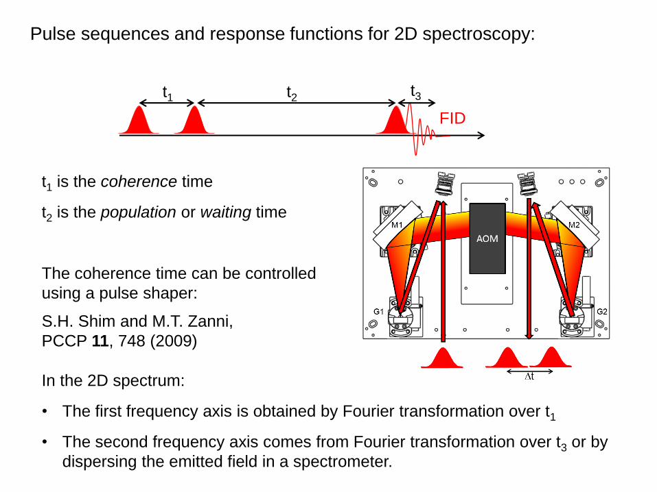
Pulse sequences and response functions for 2D spectroscopy:

t1 t2 t3

FID

In the 2D spectrum:

• The first frequency axis is obtained by Fourier transformation over t1

• The second frequency axis comes from Fourier transformation over t3 or by

dispersing the emitted field in a spectrometer.

t1 is the coherence time

t2 is the population or waiting time

The coherence time can be controlled

using a pulse shaper:

S.H. Shim and M.T. Zanni,

PCCP 11, 748 (2009)

v=0v=1

v=2

Example for a single vibrational mode: One possible Feynman pathway is

0 1

2

0 0 1 0 1 0 0

1 1 0

t1

t2

𝑅(3) 𝑡1, 𝑡2, 𝑡3 ∝ 𝑖𝜇104 𝑒𝑖𝜔10𝑡1𝑒−𝑡1/𝑇2𝑒−𝑡2/𝑇1𝑒−𝑖𝜔10𝑡3𝑒−𝑡3/𝑇2

Population relaxation

during t2

Coherence dephasing during t1 and t3

𝑆(3) 𝜔1, 𝑡2, 𝜔3 ∝ 0

∞

0

∞

𝑖𝑅(3) 𝑡1, 𝑡2, 𝑡3 𝑒𝑖𝜔3𝑡3𝑒𝑖𝜔1𝑡1𝑑𝑡1𝑑𝑡3

Coherence oscillates at

frequency 10 during periods t1and t3

𝑆(3) 𝜔1, 𝑡2, 𝜔3 ∝ 0

∞

0

∞

𝑖𝑅(3) 𝑡1, 𝑡2, 𝑡3 𝑒𝑖𝜔3𝑡3𝑒𝑖𝜔1𝑡1𝑑𝑡1𝑑𝑡3

𝑆(3) 𝜔1, 𝑡2, 𝜔3 =1

𝑖 𝜔1 − 𝜔10 − 1/𝑇2∙

1

𝑖 𝜔3 − 𝜔10 − 1/𝑇2

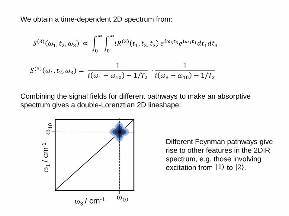
Combining the signal fields for different pathways to make an absorptive

spectrum gives a double-Lorenztian 2D lineshape:

1

/ c

m-1

3 / cm-1

1

0

10

We obtain a time-dependent 2D spectrum from:

Different Feynman pathways give

rise to other features in the 2DIR

spectrum, e.g. those involving

excitation from to . 1 2

probe (cm-1)

Transitions that contribute to a typical 2DIR spectrum of two coupled oscillators

P. Hamm and M. Zanni, Concepts and Methods of 2D Infrared Spectroscopy (Cambridge, 2011)

∆𝑖𝑗 are diagonal (𝑖 = 𝑗) and off-diagonal (𝑖 ≠ 𝑗) anharmonic shifts.

Further reading on 2D spectroscopy:

4.3 Chemical exchange observed by 2DIR

B

A

Cross peaks

emerge from

A B

exchange

Short waiting times

Long waiting times

t2 < 1 ps

t2 > 1 psP

um

p w

aven

um

ber

/ c

m-1

Pu

mp

wav

enu

mb

er /

cm

-1

Probe wavenumber / cm-1

Probe wavenumber / cm-1

BA

Reaction coordinate

Reaction coordinate

5.0 Spectral simulation using the PGOPHER program

PGOPHER is a program for simulating and fitting rotational, vibrational and

electronic spectra of molecules.

The program can be downloaded free from http://pgopher.chm.bris.ac.uk/

It is written and maintained by Dr Colin Western and a recent publication

describes its use and the underlying theory:

C.M. Western, J. Quant. Spectrosc. Radiat. Trans. 186, 221 (2016).

Guidance can be obtained from the PGOPHER website.

6.0 Conclusions

Spectroscopic methods with high frequency or time resolution provide incisive

observations of the dynamics of photochemical and chemical reactions.

These observations can be compared to the predictions of computational

studies to provide rigorous tests of theories of chemical dynamics.

The Chemical Dynamics community has the spectroscopic tools available to

impact on mechanistic understanding in other disciplines such as synthetic

chemistry, biochemistry, combustion science, solar energy capture, plasma

processing, astrochemistry and atmospheric chemistry.

Advances in spectroscopic techniques, and access to major facilities such as

synchrotrons and free electron lasers, continue to reveal new and exciting

dynamical information.