1

Phys 2310 Wed. Oct. 4, 2017Today’s Topics

– Continue Chapter 33: Geometric Optics• Reading for Next Time

2

Reading this WeekBy Monday:

Finish Ch. 33 Lenses, Mirrors and Prisms

Homework

• Due Oct. 11, 2017• Y&F Ch. 32: #32.1, 32.5

Ch. 33: #33.3, 33.7, 33.9, 33.12, 33.22, 33.24

3

4

Chapter 33: Geometric Optics

• Overview of Image Properties– No optical system produces perfect images

• Always have to choose between cost and complexity(What is the minimum cost that will still do the job?)

– Point source producing “rays of light”• An optical system producing a perfect image of source is

stigmatic. • Most real systems produce a blur spot (region of minimum

blur)– Limited by diffraction effect (later) and finite size of pixels

on the detector• Image plane vs. Object Plane (conjugate points on axis)

5

Chapter 33: Geometric Optics

• Curved Surfaces (Overview)– Purpose (goal) of an optic is to reshape wavefront

(or deflect rays) from a source to some desired shape.

• Lens: we might want to image an object onto a flat detector• Reflector: we might want to direct the light from a source

toward a given direction (flashlight beam)

– Design of an optical system depends on the goal and the requirements

– Cost is always a factor since complexity means additional labor in manufacture, mounting of components and time to completion.

6

Chapter 33: Geometric Optics

• Overview– Convex surface: surface bends outward toward the object

• Known as a converging surface or lens since light is concentrated (focused)

– Concave surface: surface bends inward away from the object• Known as a diverging surface or lens since light is less

concentrated (diverges)

• Aspherical Surfaces– Early lenses were spherical but it was known that aspherical

lenses produce the most accurate wavefronts.• Greater difficulty of manufacture and expense limits their use.

– Most common use is in parabolic reflectors and telescope mirrors• Computer design and manufacture has increased their use.

– Inclusion of a single aspherical lens in a complex optical systems can often greatly reduce its complexity

7

Chapter 33: Geometric Optics

• Spherical Surfaces– Aspheric optics function best for sources on

their axis of rotation• Off-axis sources show increased blur

(aberrations)– Geometry of spherical surfaces means that

they image over a broader “field of view”(i.e., the angular extent of the source)• Axial aberrations are present but off-axis

aberrations typically increase more slowly.– Much easier to manufacture and test

8

Supplementary: Refraction at Spherical Surfaces

• Object and Image Distances are Related– Consider a spherical convex

surface between media n and n’

– For small angles (a and g) we make a small angle approximations, the so-called paraxial rays.

– If C is opposite M r is positive and vice versa.

rnn

sn

sn

hrhnn

shn

shn

sh

rh

sh

nnnnnnnn

nnnn

-=+

-=+

@@@@

-=+®+=-

-=®+=

+=

@®=

=

'

'

'

''

'

'

''''

''

'

'

:)by through (dividing )(

:so and )tan :angles (small and ,

ing)(substitut )()TCM' triangleand for (same

MTC) triangleof angleexterior is (

)sin approx. angle (small

Law sSnell' ''sin

sin

aagba

bgabagb

bgbfgfb

fbaf

ffff

ff

9

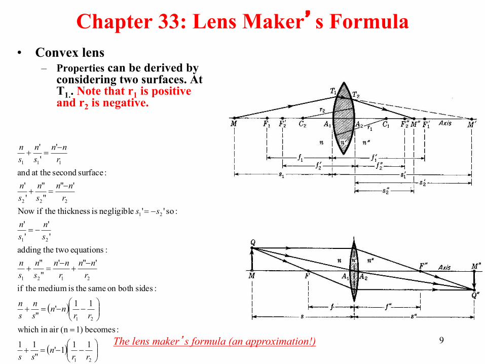
Chapter 33: Lens Maker’s Formula• Convex lens

– Properties can be derived by considering two surfaces. At T1.. Note that r1 is positive and r2 is negative.

( )

( ) ÷÷ø

öççè

æ--=+

=

÷÷ø

öççè

æ--=+

-+

-=+

-=

-=

-=+

-=+

21

21

2121

21

21

222

111

111'"

11

:becomes 1)(nair in which

11'"

:sidesboth on same theis medium theif

'"'""

:equations two theadding''

''

:so '' negligible is thickness theif Now

'"""

''

:surface second at the and

'''

rrn

ss

rrnn

sn

sn

rnn

rnn

sn

sn

sn

sn

ssrnn

sn

sn

rnn

sn

sn

The lens maker’s formula (an approximation!)

10

Chapter 33: Gaussian Optics• Recall that in deriving the Lens Maker’s Equation (aka, the

Thin Lens Equation) we made the small angle approximation:

sin f ~ f• This is also known as first-order theory since we can see

that this approximation comes from a Taylor Expansion of the Sin:

...!6!4!2

1cos

...!7!5!3

sin

642

753

+-+-@

+-+-@

ffff

fffff

If we approximate sin f ~ f – f3/3 this is known as third-order theory (i.e., there is no second-order theory for sin!)

11

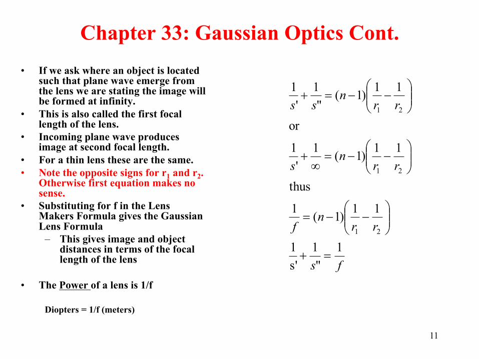
Chapter 33: Gaussian Optics Cont.• If we ask where an object is located

such that plane wave emerge from the lens we are stating the image will be formed at infinity.

• This is also called the first focal length of the lens.

• Incoming plane wave produces image at second focal length.

• For a thin lens these are the same.• Note the opposite signs for r1 and r2.

Otherwise first equation makes no sense.

• Substituting for f in the Lens Makers Formula gives the Gaussian Lens Formula

– This gives image and object distances in terms of the focal length of the lens

• The Power of a lens is 1/f

Diopters = 1/f (meters)

fs

rrn

f

rrn

s

rrn

ss

1"

1s'1

11)1(1

thus

11)1(1'

1

or

11)1("

1'

1

21

21

21

=+

÷÷ø

öççè

æ--=

÷÷ø

öççè

æ--=

¥+

÷÷ø

öççè

æ--=+

12

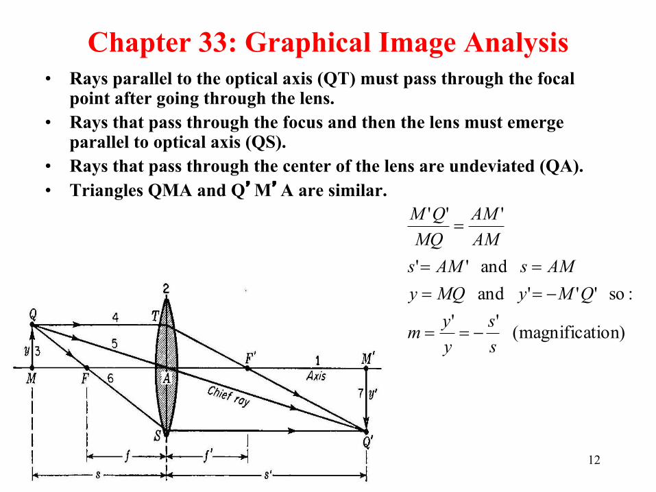
Chapter 33: Graphical Image Analysis• Rays parallel to the optical axis (QT) must pass through the focal

point after going through the lens.• Rays that pass through the focus and then the lens must emerge

parallel to optical axis (QS).• Rays that pass through the center of the lens are undeviated (QA).• Triangles QMA and Q’M’A are similar.

tion)(magnifica '':so ''' and

and ''

'''

ss

yym

QMyMQyAMsAMs

AMAM

MQQM

-==

-====

=

13

Chapter 33: Virtual Images

• Concave or Negative lenses produce de-magnified virtual images.– Trace back rays 6/7 & 8

• Objects closer than the f.l. to a positive lens produce a virtual (but magnified) image.– Trace back rays 4/5 & 6– This is the magnifying

glass!

14

Chapter 33: Thin Lens Combinations• For lens combinations the object for the second lens is just the image

formed by the first (subtract or add separation accordingly).– Be careful about the sign of the object distance (see table 5.2)– See pgs. 167-169 in Hecht for equations and the slide below.

• For the graphical method– You can solve lenses graphically by laying them out in a drawing program

(or even graph paper!) and tracing the Paraxial and Chief rays– Note that the “extra” ray (#9/10) goes through center of second lens.– In addition, ray #6/7 is deviated by second lens and must go through F’2 so

together they (#6/7 & # 9/10) locates the new image.

15

Chapter 33: Thin Len Combinations - II

• If the second lens is inside the focus of the first:– Convex lens shortens

the focal length (power is higher, neg. obj. distance for 2nd)

– Concave lens lengthens the focal length (power is increased , neg. obj. distance 2nd)

16

Chapter 33: Thin Len Combinations - III

• Gaussian lens equation can be applied to a sequence of lenses: just let the image of the first lens be the object of the second and so on.

)()( b.f.l.

)()( f.f.l.

:becomen then combinatio for the lengths focal twoThe)/()/(

:for ngsubstituti and )(

)(

:for ngsubstitutiupon and

or, 111:so and

#2) lens beyond is image theif negative becan this(Note :lens second for the Now

or, 111:LensFirst For the

21

12

21

21

11112

1111222

121

212

222

222

222

12

11

111

111

ffdfdf

ffdfdf

fsfsfdfsfsfdfs

sfsdfsds

sfsfss

sfs

sds

fsfss

sfs

oo

ooi

ii

ii

oo

oi

oi

io

o

oi

oi

+--

=+--

=

-----

=

---

=

-=

-=

-=

-=

-=

17

Chapter 33: Thin Lens in Contact

• For lens in contact (separation is negligible)– Object distance of lens #2 = Image distance of lens

#1 (let d -> 0 in b.f.l. equation above• For an object at infinity:

power)each of sum is(power

111

:or 111

21

21

21

PPPfff

fff

+=

+=

=+-

18

Chapter 33: Image Properties - I

Sign Conventions(very important, memorize!)

19

Chapter 33: Image Properties

Convex vs. Concave Lenses

20

Example Problems

• Consider a bi-convex lens with R1 = R2 = 15cm.a) Determine the focal length of the lensb) Find the image distance for an object located 35cm from

the lensc) Make a ray diagram sketch for this configurationd) Make a sketch of the image distance vs. object distance

21

Example Problems

• Consider a concave spherical mirror with fl = 60cm.

a) Is the image real or virtual?b) Find the image of an object located 10.0 m away from

the mirrorc) Make a ray diagram sketch for this configuration

• Repeat this example for a convex spherical mirror with fl = - 60cm

Homework

• Due Oct. 11, 2017• Y&F Ch. 32: #32.1, 32.5

Ch. 33: #33.3, 33.7, 33.9, 33.12, 33.22, 33.24

22

23

Reading this WeekBy Monday:

Finish Ch. 33 Lenses, Mirrors and Prisms