Atmos. Chem. Phys., 15, 2185–2201, 2015

www.atmos-chem-phys.net/15/2185/2015/

doi:10.5194/acp-15-2185-2015

© Author(s) 2015. CC Attribution 3.0 License.

Real-case simulations of aerosol–cloud interactions

in ship tracks over the Bay of Biscay

A. Possner1, E. Zubler2, U. Lohmann1, and C. Schär1

1Institute for Atmospheric and Climate Science, ETH Zurich, Zurich, Switzerland2Federal Office of Meteorology and Climatology MeteoSwiss, Zurich, Switzerland

Correspondence to: A. Possner (anna.possner@env.ethz.ch)

Received: 18 September 2014 – Published in Atmos. Chem. Phys. Discuss.: 24 October 2014

Revised: 21 January 2015 – Accepted: 31 January 2015 – Published: 27 February 2015

Abstract. Ship tracks provide an ideal test bed for study-

ing aerosol–cloud interactions (ACIs) and for evaluating their

representation in model parameterisations. Regional mod-

elling can be of particular use for this task, as this approach

provides sufficient resolution to resolve the structure of the

produced track including their meteorological environment

whilst relying on the same formulations of parameterisations

as many general circulation models. In this work we simulate

a particular case of ship tracks embedded in an optically thin

stratus cloud sheet which was observed by a polar orbiting

satellite at 12:00 UTC on 26 January 2003 around the Bay of

Biscay.

The simulations, which include moving ship emissions,

show that the model is indeed able to capture the struc-

ture of the track at a horizontal grid spacing of 2 km and

to qualitatively capture the observed cloud response in all

simulations performed. At least a doubling of the cloud opti-

cal thickness was simulated in all simulations together with

an increase in cloud droplet number concentration by about

40 cm−3 (300 %) and decrease in effective radius by about

5 µm (40 %). Furthermore, the ship emissions lead to an in-

crease in liquid water path in at least 25 % of the track re-

gions.

We are confident in the model’s ability to capture key pro-

cesses of ship track formation. However, it was found that

realistic ship emissions lead to unrealistic aerosol perturba-

tions near the source regions within the simulated tracks due

to grid-scale dilution and homogeneity.

Combining the regional-modelling approach with compre-

hensive field studies could likely improve our understanding

of the sensitivities and biases in ACI parameterisations, and

could therefore help to constrain global ACI estimates, which

strongly rely on these parameterisations.

1 Introduction

Since their discovery in satellite imagery, ship tracks have

been viewed as convincing evidence of aerosol–cloud inter-

actions (ACIs) occurring in shallow, marine planetary bound-

ary layers (PBLs). Their exclusive existence within a nar-

row range of environmental conditions despite vast global

emissions of ship exhaust has inspired a wide field of exper-

imental and modelling research on the influence of aerosol

perturbations on cloud microphysics and the marine PBL

state. Since marine shallow clouds are particularly effective

in modulating the radiative budget as well as the hydrological

cycle (Stevens and Feingold, 2009), the role of anthropogenic

emissions for these clouds is of particular interest not only for

process understanding, but also for climate impacts.

In particular it has been shown in both satellite observa-

tions (Christensen and Stephens, 2011; Chen et al., 2012;

Goren and Rosenfeld, 2012) and modelling studies (Wang

et al., 2011; Kazil et al., 2011; Berner et al., 2013) that

changes in the background aerosol and cloud condensa-

tion nuclei (CCN) concentrations not only affect the cloud

albedo by producing more numerous and smaller cloud

droplets (Twomey effect, 1974), but may also induce tran-

sitions between cloud regimes, which fundamentally change

the boundary layer state.

While CCN injections were found to induce transitions

from open- to closed-cell stratocumulus by suppressing driz-

zle formation (Wang et al., 2011; Goren and Rosenfeld,

Published by Copernicus Publications on behalf of the European Geosciences Union.

2186 A. Possner et al.: Ship track simulations over the Bay of Biscay

2012), the converse was simulated in the case of aerosol de-

pletion by precipitation. The scarcity of CCN induced the

collapse of the boundary layer and a break-up of the stratocu-

mulus cloud deck into an open cell structure with scattered,

drizzling shallow cumuli (Ackerman et al., 1993; Wood et al.,

2011; Berner et al., 2013).

Despite significant impacts of ship tracks on the re-

gional and local scale, their radiative forcing on the global

scale was found to be insignificant due to their rare occur-

rence (Schreier et al., 2007; Peters et al., 2011, 2014). As-

sessing the global effects of ACIs due to ship emissions in

general and their relevance to climate has been challeng-

ing in both satellite observations and global models. Peters

et al. (2011) found no statistically significant impacts on

large-scale cloud fields by shipping emissions using satel-

lite observations. However, due to the large natural variability

within the cloud systems which might mask potentially rel-

evant ACIs, satellite observations (Peters et al., 2014) could

not exclude their existence either.

Global general circulation model (GCM) simulations yield

globally averaged ACIs due to ship emissions between −0.6

and −0.07 Wm−2 (Lauer et al., 2007; Righi et al., 2011; Pe-

ters et al., 2012; Partanen et al., 2013). Given the maximum

simulated cooling effect, ACI induced by shipping emissions

could significantly contribute to the current best estimate of

globally averaged ACI (−0.45 Wm−2, Myhre et al., 2013).

However, ACI are represented in GCMs by parameterisa-

tions, which are highly uncertain. Combined with the limited

ability of GCMs to simulate mesoscale circulations and low

clouds in general (Nam et al., 2012), these estimates can be

given with limited confidence only.

In order to gain a more detailed understanding of the pa-

rameterised cumulative response of dynamical and micro-

physical processes to aerosol perturbations by ship emis-

sions, we consider the regional modelling approach. While

both boundary layer and microphysical processes are repre-

sented by similar parameterisations in regional models as in

GCMs, one should be able to capture the structure of a ship

track at kilometre-scale resolution. Therefore, this approach

allows for a direct comparison of the simulated ACI to ob-

servations and can hence aid significantly to constrain the

realism of the parameterised response.

In this study we use the regional COSMO model to sim-

ulate the most prominent case of ship tracks observed over

Europe by the MODIS satellite on 26 January 2003. At

12:00 UTC, the polar-orbiting satellite passed over this re-

gion and captured ship tracks embedded within optically thin

stratus (optical thickness τ ≤ 2) west of the Bay of Biscay

(see Fig. 1). From the satellite image one can deduce further

information on the background conditions of the boundary

layer.

Based on the structures of open cells underneath the op-

tically thin cloud layer visible in the MODIS image, one

can infer the cloud to be drizzling. To the east of the ship

track region, a closed stratocumulus deck without any ship

track signal was observed. This is consistent with our current

understanding of the susceptibility of different cloud sys-

tems to aerosol perturbations (Stevens and Feingold, 2009).

While drizzling boundary layers of little cloud water have

previously been identified as susceptible to aerosol perturba-

tions, optically thick non-precipitating stratocumulus sheets

are known to buffer the response to the aerosol perturbation

(e.g. Coakley et al., 1987; Stevens and Feingold, 2009; Chen

et al., 2012; Christensen and Stephens, 2012).

Furthermore the presence of the optically thin stratus sug-

gests the boundary layer to be weakly mixed in this region

as the cloud top radiative cooling is small. This is supported

by soundings at the French coast at Brest, which display a

collapsed boundary layer structure with a strong inversion

of 12 K at 500 m on 27 January 2003 at 00:00 UTC (Poss-

ner et al., 2014). The collapse of the marine boundary layer

with a remnant stratified thin cloud layer has been found to

coincide with aerosol deprived clean background conditions

due to precipitation scavenging of CCN where cloud droplet

numbers can be as low as 1–10 cm−3 (Ackerman et al., 1993;

Wood et al., 2011; Berner et al., 2013).

In these simulations the response of the aerosol and cloud

bulk microphysics parameterisations to the ship emissions

are quantified and discussed in the context of the MODIS ob-

servation and other ship track measurements from the liter-

ature. Additionally, parameterised boundary layer processes,

such as PBL tracer transport, are discussed as well as the im-

pact of the ship exhaust on the PBL structure.

2 Methods

2.1 Model description

The simulations were carried out with the COSMO model,

developed and maintained by the COSMO consortium. The

COSMO model (version 4.14) is a state-of-the-art, non-

hydrostatic model used at 2 km horizontal resolution with a

time step of 20 s. A vertical resolution of at most (resp. at

least) 150 m (20 m) in the PBL was used. The fully compress-

ible flow equations are solved using a third-order Runge–

Kutta discretisation in time (Wicker and Skamarock, 2002;

Foerstner and Doms, 2004). Vertical advection is computed

using an implicit second-order centred scheme and hori-

zontal advection is solved using a fifth-order upstream dis-

cretisation. Tracers, such as the hydrometeors and aerosol

species, are advected horizontally using a second-order Bott

scheme (Bott, 1989). The turbulent fluxes are represented

using a 1-D turbulent diffusion scheme with a prognostic

description for the turbulent kinetic energy. The minimum

threshold for the eddy diffusivity intrinsic to the turbulence

parameterisation is set to 0.01 m2 s−1 (Possner et al., 2014).

Shallow convection is described using the Tiedtke (1989)

mass flux scheme without precipitation production with an

entrainment rate of 3× 10−4 m−1. The radiative transfer is

Atmos. Chem. Phys., 15, 2185–2201, 2015 www.atmos-chem-phys.net/15/2185/2015/

A. Possner et al.: Ship track simulations over the Bay of Biscay 2187

pre-

front

al c

onve

ctiv

e ba

nd

ship tracks

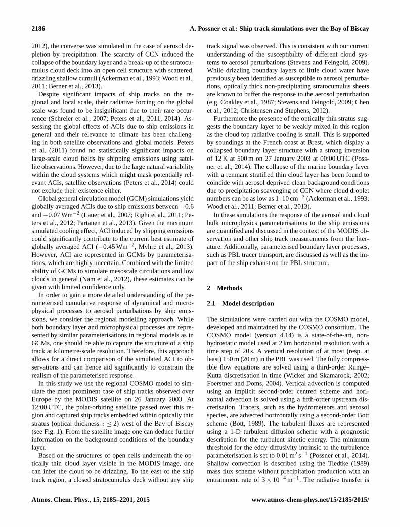
Figure 1. True-colour MODIS satellite image (wavelength bands 670, 565 and 479 nm) on 26 January 2003 at 12:00 UTC of the Bay of

Biscay. Note the numerous ship tracks in the northwest of the image and the pre-frontal band of convection stretching across the Bay.

based on a δ-two-stream approach (Ritter and Geleyn, 1992)

using a relative humidity criterion for subgrid-scale cloud

cover.

In previous work the model was extended with a two-

moment bulk cloud microphysics scheme (Seifert and Be-

heng, 2006) and the M7 aerosol microphysics scheme (Vi-

gnati et al., 2004; Zubler et al., 2011). The aerosol micro-

physics scheme describes the evolution of black carbon (BC),

organic carbon (OC), sulfate (SO4), sea salt and dust. These

species are binned into four internally mixed soluble and

three insoluble modes determined by fixed size ranges (nu-

cleation, Aitken, accumulation and coarse). The processes

relevant to this study captured by the model include con-

densation of sulfuric acid vapour, hydration, coagulation,

sedimentation as well as dry and wet deposition of aerosol

particles. The soluble aerosol particles are activated accord-

ing to Lin and Leaitch (1997). All soluble aerosol particles

in the accumulation (50nm≤ R ≤ 0.5 µm) and coarse (R >

0.5 µm) mode, as well as Aitken mode (5nm≤ R ≤ 50 nm)

aerosol particles larger than 35 nm radius are considered as

activated. Although there exist more physical activation pa-

rameterisations (e.g. Abdul-Razzak and Ghan, 2000; Nenes

and Seinfeld, 2003), using this simpler form of activation is

still in good agreement with observations, which found the

CCN concentration to scale linearly with the soluble accumu-

lation mode number concentration (Wood, 2012 and refer-

ences therein). The number of newly activated cloud droplets

is then further restricted by the available moisture content

and the updraft velocity (Lohmann, 2002).

The cloud microphysical processes for cloud droplets and

rain described by the Seifert and Beheng (2006) parameter-

isation contain the growth by condensation, self-collection

of cloud droplets and rain drops, autoconversion, accretion,

droplet breakup, sedimentation of rain and evaporation (sat-

uration adjustment is applied). The grid-scale cloud optical

properties are parameterised as a function of wavelength us-

ing the effective droplet radius (Hu and Stamnes, 1993).

2.2 Numerical experiments

The dynamical settings and nesting approach used in these

simulations are based on the setup of Possner et al. (2014).

We use a one-way nesting approach, where the 2 km simula-

tion (1t = 20 s) is nested in a 12 km simulation (1t = 90 s)

run over a larger domain stretching from the northeast At-

lantic to the eastern borders of Switzerland and Germany

(see Fig. 1 of Possner et al., 2014). The initial and lateral

boundary conditions for the dynamical fields are provided

by the ECMWF Interim Reanalysis (Uppala et al., 2005;

Dee et al., 2011). For the aerosol tracers, the climatolog-

ical means for January (1999–2009) obtained in ECHAM-

HAM simulations (Folini and Wild, 2011) are prescribed as

initial and lateral boundary conditions. The global simula-

tions were performed with a two-moment bulk scheme for

aerosol (Stier et al., 2005) and cloud (Lohmann et al., 2007)

www.atmos-chem-phys.net/15/2185/2015/ Atmos. Chem. Phys., 15, 2185–2201, 2015

2188 A. Possner et al.: Ship track simulations over the Bay of Biscay

microphysics with prescribed aerosol and precursor emis-

sions from the Japanese National Institute for Environmen-

tal Studies (NIES, Roeckner et al., 2006; Stier et al., 2006;

Nozawa et al., 2007).

In the present simulations, anthropogenic aerosol emis-

sions, excluding ship emissions, are given by the AeroCom

data set (Kinne et al., 2006). Natural emissions such as

dimethylsulfide (DMS) emissions (Zubler et al., 2011) and

sea salt (Guelle et al., 2001) emissions are computed interac-

tively.

2.2.1 Shipping emissions

By combustion of low-quality fuel ships emit gases such as

SO2, NO2, hydrocarbons and carbon monoxide, and partic-

ulate matter (PM) such as SO4, OC, BC and ash into the at-

mosphere.

However, of the gaseous emissions only SO2 is considered

in this study, which focuses solely on aerosol–cloud interac-

tions (ACI) of ship emissions. Although emitted hydrocar-

bons, as well as CO, lead to significant increases of green-

house gas concentrations (CH4 and CO2 respectively), their

contribution to aerosol mass and number concentrations is

small (Murphy et al., 2009). As the secondary aerosol forma-

tion of nitrates in sulfur-rich emissions is also very small (Vu-

tukuru and Dabdub, 2008; Murphy et al., 2009), NO2 emis-

sions were not prescribed. Furthermore, ash emissions are

also not included as ash particles are too small in number

due to their large size (∼ 200 nm to 10µm, Moldanová et al.,

2009) to contribute significantly to the CCN concentration

and were not measured in the two field campaigns (Hobbs

et al., 2000; Lack et al., 2009) used for the emission specifi-

cation of this study.

The emission fluxes used in this study are based on mea-

surements of cargo ship emissions obtained in the Mon-

terey Area Ship Track campaign (Hobbs et al., 2000). Cargo

ships, such as tankers, bulk carriers, container and passen-

ger ships larger than 100 gross tons, contribute to 50 % of

the global fleet and are the major source of global ship-

ping emissions (Corbett, 2003). The PM emission fluxes for

BC, OC and SO4 are based on the mean PM particle num-

ber emission flux of five different cargo vessel measure-

ments (Hobbs et al., 2000). The mean total particle num-

ber flux (9× 1015 s−1) was chosen, as individual emission

measurements themselves varied by more than a factor of 2

between the individual vessels. The PM mass flux was esti-

mated using the total particle number flux and estimates of

emission size and density. For each of the five considered

ships, the median emission radius was provided by Hobbs

et al. (2000). The averaged median radius (0.04 µm) was

used as the emission size estimate for all particles. Together

with the density estimate, which was taken as the mean den-

sity across all involved constituents (∼ 1.95 gcm−3), the PM

mass flux was approximated as 20.84 kgh−1. In a final step

the emission fluxes for OC (9.59 kgh−1), BC (3.13 kgh−1)

Table 1. Specifications of the two size distributions used for ship

emission fluxes obtained from Righi et al. (2011). The ship emis-

sions are treated as lognormal size distributions and are partitioned

into the soluble Aitken (AIT) and accumulation (ACC) modes based

on the mass percentage at the mean radius R̄.

Fresh Aged

AIT ACC AIT ACC

R̄ [µm] 0.015 – 0.029 0.16

% [mass] 100 0 96 4

and SO4 (8.13 kgh−1) were determined using the mass frac-

tions of ship emissions measured by Lack et al. (2009). The

SO2 emission flux (144 kgh−1) was inferred from Hobbs

et al. (2000) by averaging the five vessel measurements.

In the present simulations, the PM and SO2 emission mass

fluxes were emitted in one level ∼ 160 m above the surface

(e.g. Peters et al., 2012) with a log-normal size distribution

(σ = 1.59) and two different size specifications (Righi et al.,

2011; Lund et al., 2012) shown in Table 1. Both size distri-

butions, fresh and aged, are inferred from measurements and

attempt to include coagulation effects of the aerosol as time

progresses. They differ in the partitioning of the emission

fluxes between the Aitken and the accumulation size modes.

Whereas the size distribution of the fresh emissions is repre-

sentative for emissions at the ship’s exhaust where all aerosol

particles are emitted into the Aitken mode, the aged size dis-

tribution represents older emissions where coagulation pro-

cesses occurred and the aerosol particles are split into the

Aitken (96 %) and accumulation (4 %) modes.

We prescribe three ships starting at 03:00 UTC on 26 Jan-

uary 2003 at the same longitude at the edge of the Bay of

Biscay, arbitrarily separated in their initial position in the

latitude by 50 km (between the northernmost and middle

ship) and 80 km (between middle and southernmost ship).

All ships move southwest at 230◦ (0◦ pointing north) at 5,

10, or 20 ms−1. For numerical stability the ship exhaust is

not emitted into a single grid box, but distributed horizontally

into four adjacent grid boxes (Fig. 2), based on the ship’s ex-

act location, scaled by the distance-weighted mean.

Whilst all boundary fields are updated at an hourly rate, the

ship emission fields are updated every 3 minutes. For each 3-

minute interval the ship emissions are accumulated within

the four adjacent grid points around the instantaneous ship

position.

The performed simulations, summarised in Table 2, in-

clude a control run (clean) where the contribution of shipping

emissions is zero and a simulation where the ship emissions

are specified as described above (ship). As discussed in detail

in Sect. 3.1, the emission flux by Hobbs et al. (2000) gener-

ated smaller aerosol perturbations near the emission source in

the ship simulation than the measurements of aerosol num-

ber concentration obtained in the same study. We therefore

Atmos. Chem. Phys., 15, 2185–2201, 2015 www.atmos-chem-phys.net/15/2185/2015/

A. Possner et al.: Ship track simulations over the Bay of Biscay 2189

tt + 3'

Figure 2. 2 km simulation domain of 1160km× 800km showing

three prescribed ship routes oriented from northeast to southwest.

A schematic of the distribution of the ship emissions along the

2 km× 2km grid is given inside the black box. The emissions are

distributed at a 3 min (1.5 min) interval within four adjacent grid

boxes along the ship’s route for ships moving at 5 or 10 ms−1

(20 ms−1). The red box displays the ship track domain used in

Figs. 3–7 and 9. (Note that the ship plume locations shown in these

figures are determined by the relative motion between the ships and

the horizontal wind.)

Table 2. Summary of ship emission specifications as prescribed in

the simulations. Prescribed SO2 and PM mass fluxes based on the

literature (Hobbs et al., 2000) are given together with prescribed

size distributions and ship’s speed (vship).

Simulation SO2 flux PM flux Size vship

[kgh−1] [kgh−1] distribution [ms−1]

clean – – – –

ship 144 20.84 fresh 10

ship10 144 208.4 fresh 10

ship10A 144 208.4 aged 10

ship10_V5 144 208.4 fresh 5

ship10_V20 144 208.4 fresh 20

perform experiments with scaled emission mass fluxes by a

factor 10 (ship10). A scaling of similar order of magnitude

has been applied in a previous study performed at consider-

ably higher resolution, where the aerosol perturbation gener-

ated by emissions from Hobbs et al. (2000) were found to be

insufficient to create a significant cloud response (Wang and

Feingold, 2009).

The necessity for such a scaling may be due to the dilu-

tion of a point source emission onto the grid scale, which

may lead to a biased representation of the subsequent micro-

physical processing of the plume. However, it may also be

needed due to possible measurement biases, which are partic-

ularly likely to occur near the emission source, as the aerosol

concentrations vary rapidly with the plume’s cross-sectional

radius in this part of the plume.

In addition, the sensitivity towards the emission parti-

cle size is investigated in ship10A, where the aged emis-

sion size distribution is prescribed. Furthermore, simulations

with varied ship speeds are performed in order to under-

stand the balance of the macrophysical constraints (e.g. cloud

cover and moisture availability) and the microphysical feed-

backs involved in determining the extent of the ship tracks.

Whereas the ships move at 10 ms−1 in most simulations, the

ships’ speed was set to 5 ms−1 in ship10_V5 and 20 ms−1 in

ship10_V20. In doing so, one can assess the influence of the

ship’s speed on the track structure.

2.3 Classification of ship plume

In order to quantify the changes in microphysical entities,

a distinction between plume and non-plume grid points has

to be made in the post-processing. As the only perturbation

in total aerosol number concentration Na is caused by ship

emissions, we defined a relative threshold concentration of

Na at each grid point to determine the plume points. Only

points where Nasimulation≥ 3Naclean

are considered part of the

ship exhaust plume. This threshold provides the required bal-

ance of being small enough to include a maximum num-

ber of plume points and being large enough to separate the

core track structures from surrounding increases of Na due

to aerosol being mixed away from the track region.

Another sampling was performed to determine not only

the plume points, but the subset of plume points where a sig-

nificant cloud response was detected. Here, the additional cri-

terion in terms of cloud droplet number concentration Nc of

Ncsimulation≥ 5Ncclean

was applied.

The ability to distinguish plume from non-plume points

and ship track from non-ship-track points of these criteria is

shown in Sect. 3.4.

2.4 Evaluation of cloud optical thickness

A simple metric to compare simulated cloud optical thick-

ness to the MODIS observation was designed, as the COSP

simulator (Bodas-Salcedo et al., 2011), including grid-scale

and subgrid-scale cloud water contributions, is not yet avail-

able within COSMO.

Cloud optical thickness τ within COSMO is diagnosed for

each of the eight spectral intervals (three shortwave and five

longwave) in the radiation scheme. For warm-phase clouds τ

is given as

τ(x,y,λi)=

TOA∫0

ξ (λi)qctot(x,y,z)clctot(x,y,z)dz, (1)

where ξ (λi) denotes the extinction coefficient of each spec-

tral band λi , qctot the total (grid-scale and subgrid-scale) liq-

uid water content at each grid point at coordinates x (lon-

gitude), y (latitude) and z (level), and clctot the cloud cover

fraction (predominantly 0 or 1 in these simulations).

As MODIS cloud optical thickness during day-time and

over the ocean is predominantly defined by radiances mea-

www.atmos-chem-phys.net/15/2185/2015/ Atmos. Chem. Phys., 15, 2185–2201, 2015

2190 A. Possner et al.: Ship track simulations over the Bay of Biscay

sured within the visible (King et al., 1998; Platnick et al.,

2003), the contribution of the visible channel in COSMO

(0.25≤ λ≤ 0.7µm) to the total τ was isolated and used for

the MODIS comparison.

3 Results

Before a detailed assessment of the ship exhaust effects on

the stratocumulus deck is given in the following sections, the

background state is described. The mesoscale circulations

and the macrophysical state on 26 January are predominantly

driven by an extensive high-pressure system with an under-

lying subsidence rate of about −0.75 cms−1 at night and

−0.25 cms−1 during daytime at a height of 1.5 km. Tempera-

ture gradients of up to 4 K per 100 m are simulated within the

inversion in the ship track domain (domain shown in Fig. 2).

An inversion of this magnitude was only obtained after a sig-

nificant reduction of the prescribed minimum threshold for

the eddy diffusivity of heat and moisture from the operational

value of 1.0 to 0.01 m2 s−1 (Possner et al., 2014). A detailed

evaluation using coastal soundings of PBL profiles of hor-

izontal wind, potential temperature θ and relative humidity

and their impact on cloud cover is presented in Possner et al.

(2014).

The horizontal large-scale advection of the air masses is

dominated by northwesterly flow, pushing air masses from

the ship track region towards the continent. During the sim-

ulated period a pre-frontal band of organised convection (see

Fig. 1) propagates through the domain from the northwest to

the east and passes through the ship track domain between

07:00 and 12:00 UTC.

3.1 Impacts on aerosol microphysics

The simulated background of this case study is very clean

due to the presence of unpolluted marine air into the ship

track domain and the removal of aerosol by precipitation.

Aerosol concentrations as low as 285 cm−3 and CCN con-

centrations of 10–20 cm−3 are simulated.

The background aerosol particles are a composite of sea

salt emitted within the region and sulfate particles within the

Aitken mode, which are transported into the domain from the

lateral boundaries. The sulfate particles formed in the mid-

troposphere and were mixed downward in the driving GCM

simulations. Although the aerosol and CCN concentrations

are low, they are not unrealistic for this region (Zubler et al.,

2011) or for stratocumulus in general (Wood, 2012) and are

consistent with the MODIS observation of optically thin stra-

tus.

The impact of the ship exhaust in all simulations, contain-

ing either a varied emission mass flux (ship10) or emission

size (ship10A), on the aerosol size distribution is illustrated

in Fig. 3. This figure shows the averaged aerosol size distri-

butions determined over a plume volume close to the source

at 06:00 UTC and at a distance at 12:00 UTC. The selection

method of the included plume grid points of each track is

illustrated in Fig. 4. At each of these points the size dis-

tribution is determined and then bin-wise averaged over all

selected plume points. As in situ size distribution measure-

ments shown in Fig. 3 are obtained within a 10 km radius

of the ship’s position, plume points within the same radius of

each ship are selected at 06:00 UTC. Furthermore, to ensure a

comparison of the same volume of air between different sim-

ulations, the plume points considered for this analysis were

determined in ship10 and used in all other simulations. In

order to visualise size distribution changes along the plume

due to dilution and microphysical processing, the distribu-

tions were determined again at 12:00 UTC over plume points

selected from a volume of air centred at the same latitude as

06:00 UTC (see Fig. 4) which now contains atmospherically

aged aerosol particles. To highlight the variability between

individual plume points, the span between the 10th and 90th

percentiles (P10 and P90 respectively) is shown in addition

to the averaged distribution in grey at 06:00 UTC.

In general a good agreement of the peak width is found

between all simulations and observations obtained by Hobbs

et al. (2000) (Fig. 3 blue markers) and Petzold et al. (2008)

(Fig. 3 orange markers), while peak amplitudes are underes-

timated with respect to the observations in ship and ship10A.

Observed peak concentrations in aerosol number per size bin,

which vary between 5000 cm−3 and 100 000 cm−3 (i.e. over

two orders of magnitude), are only captured by the ship10

simulation.

However, it has to be considered that the observations

shown in Fig. 3 were obtained within different marine bound-

ary layers of varying background aerosol concentrations,

ship emissions (in terms of mass flux and size) and PBL state,

and were obtained for considerably smaller samples of air

(compared to a 2 km by 2 km by 100 m volume) at different

plume ages. As all of these factors influence the plume evo-

lution, complete conformity between the simulated plumes

of this case study and the observations is not to be expected.

However, a qualitative comparison in terms of order of mag-

nitude can still be made and provides valuable insights.

In addition to size distribution measurements, observa-

tions of the total perturbation in aerosol number concentra-

tion are also considered. The simulated perturbations in Na

(1Na shown in Fig. 3b–d) are compared to measurements

obtained by Hobbs et al. (2000) (Fig. 1 of their paper) for a

bulk carrier running on marine fuel oil (Star Livorno), which

was one of the five ships considered for the ship exhaust es-

timate of this study. The observations of1Na range between

3000 and 30 000 cm−3. However, only 7 % of the measure-

ments were smaller than 5000 cm−3, while over 50 % were

obtained at 1Na > 20 000 cm−3. Therefore, peak concentra-

tions of at least 20 000 cm−3 in the vicinity of the ship can be

inferred.

In the simulations 1Na was determined at each point by

taking the difference between any simulation containing ship

Atmos. Chem. Phys., 15, 2185–2201, 2015 www.atmos-chem-phys.net/15/2185/2015/

A. Possner et al.: Ship track simulations over the Bay of Biscay 2191

a 06 UTC12 UTC

06 UTC12 UTC

06 UTC12 UTC

06 UTC12 UTC

x103 b

d x103 c

x103

Figure 3. Mean aerosol size distributions of internally mixed aerosol for (a) clean, (b) ship, (c) ship10 and (d) ship10A are shown at 06:00

and 12:00 UTC. At 06:00 UTC size distributions were averaged bin-wise near the emission source and at 12:00 UTC at a distance of 216 km

(see text for details). Red line marks the activation size threshold. In panels (b–d): grey shaded region spans between the 10th and 90th

percentiles at 06:00 UTC; field study measurements are represented by coloured markers and include five size distribution measurements

(different shades of blue) obtained by Hobbs et al. (2000) of vessels and one measurement (orange) obtained by Petzold et al. (2008); box

plot representations of the total aerosol perturbation (1Na) at 06:00 UTC near the emission source with respect to the background (obtained

from clean) are shown in addition (note their different scale).

06 UTC

12 UTC

Figure 4. Schematic of selection method for plume points consid-

ered for averaged size distributions shown in Fig. 3. Exemplary

tracks are shown for 06:00 and 12:00 UTC within the same map.

The plume points are sampled at each level within a 10 km radius

(red half circle) at the latitude (red line) defined by the ship’s posi-

tion at 06:00 UTC. Therefore the plume points contain freshly emit-

ted aerosol particles at 06:00 UTC and atmospherically aged aerosol

particles at 12:00 UTC.

exhaust and clean over plume points within a 10 km radius

from the source at 06:00 UTC. A comparison between the

simulated range of 1Na with the observations shows that al-

most 75 % of the simulated perturbations are below the ob-

served range. This indicates that the aerosol perturbation due

to the literature-scale emission flux might be insufficient to

generate comparable peak concentrations within the plume.

On the other hand, the simulated range of perturbations as

compared to the observations agrees well up to the 75th per-

centile (P75) with the observations of ship10. However, this

agreement is obtained at the expense of a considerable over-

estimation of the peak perturbations in this simulation.

In addition to differences in peak amplitude, a shift of the

aerosol peak towards smaller radii is detectable between the

ship and ship10 simulations and observations. The difference

in peak radius is strongly tied to the emission size of the

ship exhaust. Whilst an emission size of 0.015 µm was spec-

ified for fresh plumes (Table 1), ship exhaust radii of at least

0.03 µm were measured by Hobbs et al. (2000). While this

discrepancy in emission radius was noted, the results of this

study were not found to be affected.

The aerosol size distribution in ship10A displays a distinct

double-peak structure due to the bimodal emission size dis-

tribution applied (Table 1). While all observations shown in

Fig. 3 display a single peak, measurements of double-peak

structures have been obtained in test bed studies (Petzold

et al., 2008). In terms of 1Na, smaller peak perturbations

are simulated in ship10A than observed, as the aged emis-

sion size distribution was developed to represent older plume

segments, which consequentially are more diluted.

www.atmos-chem-phys.net/15/2185/2015/ Atmos. Chem. Phys., 15, 2185–2201, 2015

2192 A. Possner et al.: Ship track simulations over the Bay of Biscay

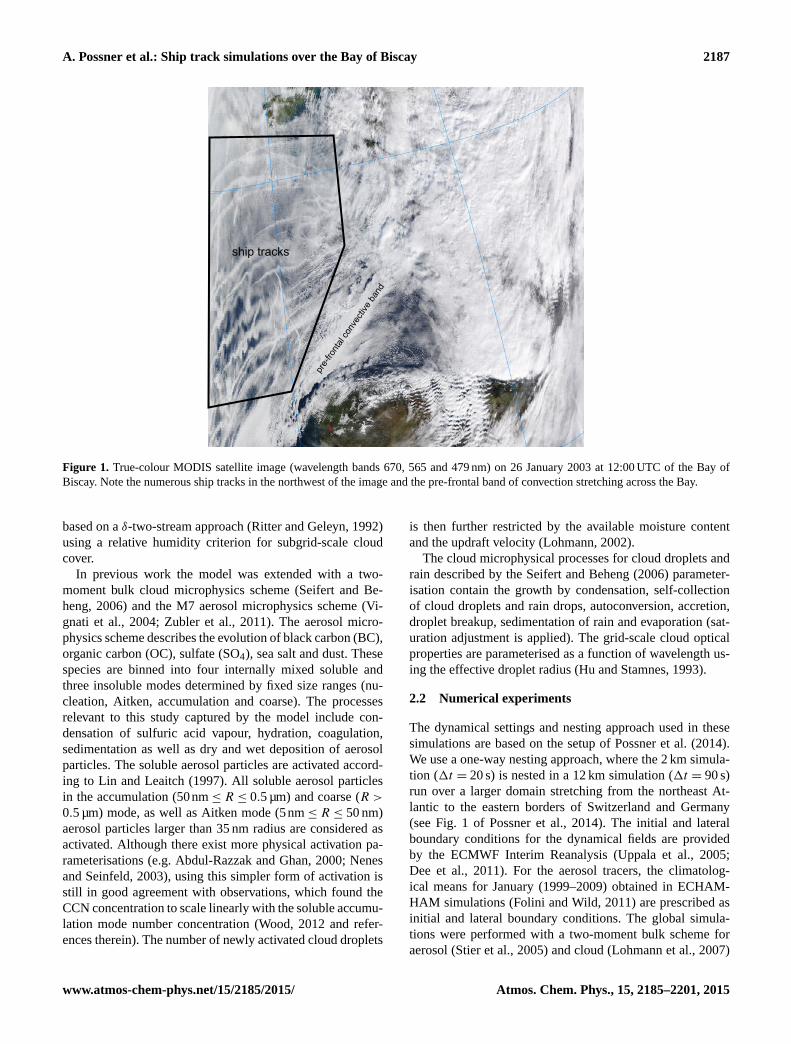
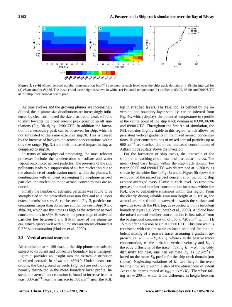
Figure 5. (a–b) Mixed aerosol number concentration [cm−3] averaged at each level over the ship track domain at a 15 min interval for

(a) clean and (b) ship10. The mean cloud base height is shown in white. (c) Potential temperature (θ ) profiles at 03:00, 06:00 and 09:00 UTC

at the ship track domain centre point.

As time evolves and the growing plumes are increasingly

diluted, the in-plume size distributions are increasingly influ-

enced by clean air. Indeed the size distribution peak is found

to shift towards the clean aerosol peak position in all sim-

ulations (Fig. 3b–d) by 12:00 UTC. In addition the forma-

tion of a secondary peak can be observed for ship, which is

not simulated to the same extent in ship10. This is caused

by the increase of background aerosol concentrations within

this size range (Fig. 3a) and their increased impact in ship as

compared to ship10.

In terms of microphysical processing, the most relevant

processes include the condensation of sulfate and water

vapour onto mixed aerosol particles. The presence of the ship

pollutants leads to a suppression of sulfate nucleation due to

the abundance of condensation nuclei within the plumes. In

combination with efficient scavenging by in-plume aerosol

particles, the nucleation mode aerosol concentrations are re-

duced.

Finally the number of activated particles was found to be

strongly tied to the prescribed emission flux and to a lesser

extent to emission size. As can be seen in Fig. 3, particle con-

centrations larger than 35 nm are similar between ship10 and

ship10A, which are five times as high as the activated aerosol

concentrations in ship. However, the percentage of activated

particles lies between 3 and 6 % in most of the plume ar-

eas, which agrees well with plume measurements obtained at

0.2 % supersaturation (Hudson et al., 2000).

3.2 Vertical aerosol transport

After emission at ∼ 160 ma.s.l., the ship plume aerosols are

subject to turbulent and convective boundary layer transport.

Figure 5 provides an insight into the vertical distribution

of mixed aerosols in clean and ship10. Under clean con-

ditions, the background aerosols (Fig. 5a) are not homoge-

neously distributed in the mean boundary layer profile. In-

stead, the aerosol concentration is found to increase from at

least 300 cm−3 near the surface to 500 cm−3 near the PBL

top in stratified layers. The PBL top, as defined by the in-

version, and boundary layer stability, can be inferred from

Fig. 5c, which displays the potential temperature (θ ) profile

at the centre point of the ship track domain at 03:00, 06:00

and 09:00 UTC. Throughout the first 9 h of simulation, the

PBL remains slightly stable in this region, which allows for

persistent vertical gradients in the mixed aerosol concentra-

tions. Higher concentrations of mixed aerosol particles up to

600 cm−3 are reached due to the increased concentration of

Aitken mode sulfate above the inversion.

For the formation of ship tracks, the timescale of the

ship plume reaching cloud base is of particular interest. The

mean cloud base height within the ship track domain be-

tween 00:00 and 09:00 UTC was determined at ∼ 360 m, as

shown by the white line in Fig. 5a and b. Figure 5b shows the

evolution of the mixed aerosol concentration including ship

exhaust averaged every 15 min at each level. As time pro-

gresses, the total number concentration increases within the

PBL, due to cumulative emissions within this region. From

the clearly distinguishable emission height at ∼ 160 m, the

aerosol are mixed both downwards towards the surface and

upwards towards the PBL top, as expected within a turbulent

boundary layer (e.g. Verzijlbergh et al., 2009). At cloud base

the mixed aerosol number concentration is first raised from

the background concentration of 350 to 420 cm−3 within 1 h

15 min after emission begin at 03:00 UTC. This timescale is

consistent with the timescale estimate obtained for the tur-

bulent mixing of a passive tracer assuming a gradient ap-

proach, i.e. w′c′ =−Kc∂c/∂z, where c is the passive tracer

concentration, w′ the turbulent vertical velocity and Kc is

the eddy diffusivity of the tracer. Taking Kc ∼Kh, the eddy

diffusivity for heat, one can estimate Kc as 12.3 m2 s−1

based on the mean Kh profile for the ship track domain (not

shown). Neglecting variations of Kc with height, the over-

turning time scale within a slab of the atmosphere of extent

1z can be approximated as τturb ∼1z2/Kh. Therefore tak-

ing 1z= 200 m, which is the difference in height between

Atmos. Chem. Phys., 15, 2185–2201, 2015 www.atmos-chem-phys.net/15/2185/2015/

A. Possner et al.: Ship track simulations over the Bay of Biscay 2193

Aclean

Bship

Dship10A

Eship10_

V5

Fship10_

V20

12 UTC09 UTC12 UTC09 UTC

Cship10

x104

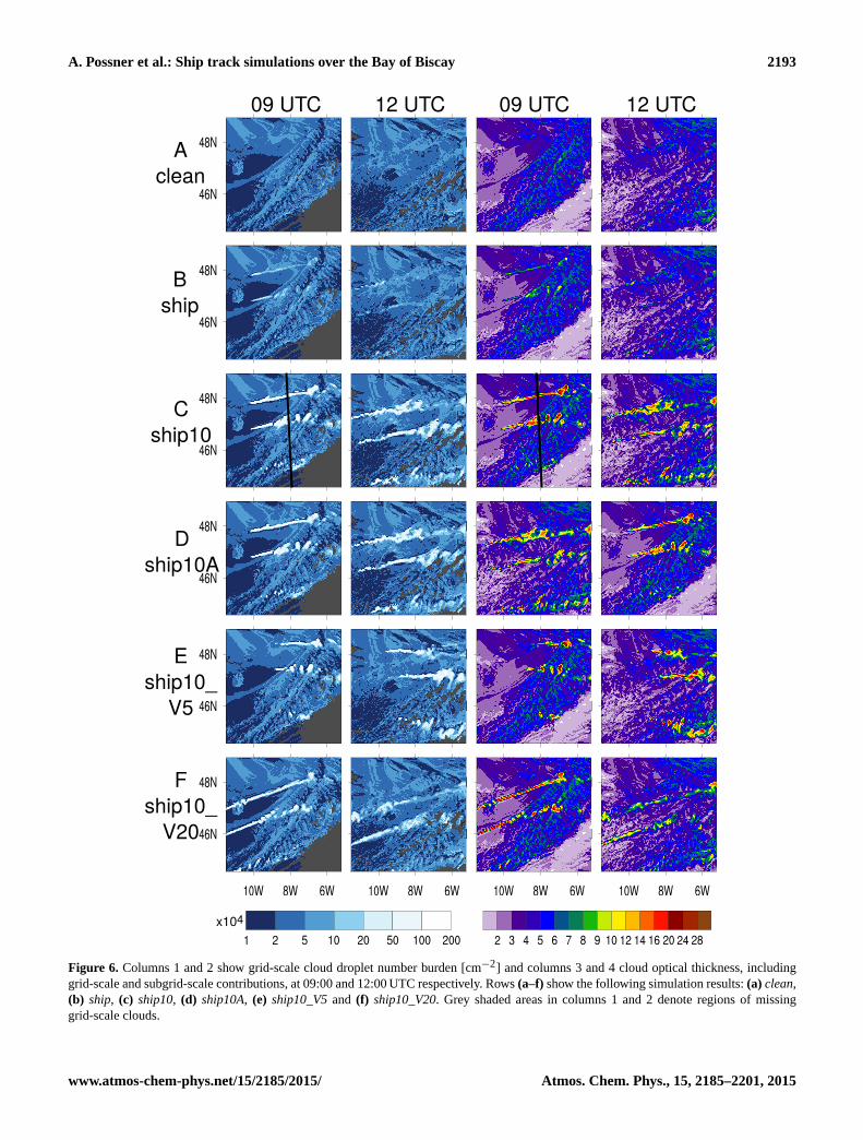
Figure 6. Columns 1 and 2 show grid-scale cloud droplet number burden [cm−2] and columns 3 and 4 cloud optical thickness, including

grid-scale and subgrid-scale contributions, at 09:00 and 12:00 UTC respectively. Rows (a–f) show the following simulation results: (a) clean,

(b) ship, (c) ship10, (d) ship10A, (e) ship10_V5 and (f) ship10_V20. Grey shaded areas in columns 1 and 2 denote regions of missing

grid-scale clouds.

www.atmos-chem-phys.net/15/2185/2015/ Atmos. Chem. Phys., 15, 2185–2201, 2015

2194 A. Possner et al.: Ship track simulations over the Bay of Biscay

a

ship shipbackground background

shipship10

ship10A

ship10_V5

ship10_V20

b c

observations

Figure 7. (a–b) Distributions across PBL grid points for either plume points of significant cloud response or environmental background

conditions are shown for (a) Nc and (b) Reff at 12:00 UTC for all simulations containing ship emissions. The box edges denote the 25th

and 75th percentiles, and the whiskers display the 5th and 95th percentiles. The plume regions were diagnosed within ship10, ship10_V5

(for ship10_V5 only) and ship10_V20 (for ship10_V20 only). The range of observations is denoted in black. Panel (c) displays the top of

the atmosphere (TOA) shortwave (SW) cloud radiative effect (CRE) averaged over the entire ship track region for all simulations (clean is

shown in light blue).

the cloud base and emission height, τturb is approximated as

54 min, which agrees well with the timescale obtained from

the mean profiles shown in Fig. 5b.

In addition to turbulent transport, a fraction of the ship

emissions are transported by convective fluxes into the cloud

layer, just below the inversion base. At the level between

500 m and inversion base height, the mixed aerosol concen-

trations are raised by 10–15 cm−3 already 30 min after emis-

sion onset. However, turbulent mixing is the predominant

form of vertical PBL transport at this time.

Finally, Fig. 5b clearly highlights the confinement of the

ship plume to the boundary layer due to the strong inversion.

The mixed aerosol concentrations above the PBL remain un-

affected by the ship emissions.

3.3 Microphysical and radiative effects

The simulated cloud microphysical response to the plumes

of increased aerosol concentration was found to be in agree-

ment with findings of previous studies. Within plume re-

gions, the increased number of activated aerosol led to an in-

crease in cloud droplet number concentration and a decrease

in effective radius. As a result, the cloud optical thickness

increased. The strength of the response is sensitive to the

plume’s age and intensity (in terms of aerosol number con-

centration) as well as the environmental conditions, as dis-

cussed in Sect. 3.4.

Figure 6 displays the cloud droplet number burden

summed over the PBL (columns 1 and 2) and τ (columns 3

and 4) at 09:00 and 12:00 UTC. For this purpose, the inver-

sion top, which lies at around 800 m, was diagnosed for each

column based on the temperature gradient (Possner et al.,

2014). Although all simulations display an increase in the

cloud droplet burden along the tracks, its extent varies sig-

nificantly among the different simulations. At 09:00 UTC,

the cloud droplet burden is increased up to 120× 104 cm−2

within the plume regions in all simulations apart from ship,

where maximum burdens of 15× 104 cm−2 are simulated.

Considering the significantly smaller number of activated

aerosol within the plume in ship (Fig. 3b), this is to be ex-

pected. After an additional 3 h of simulation, the tracks have

grown in size, but similar values of cloud droplet burden are

reached at 12:00 UTC.

In ship10_V20 however, a significant decrease in the cloud

droplet burden was simulated down to 20× 104 cm−2 un-

til 12:00 UTC. Whilst the ship tracks shown in rows 1–5

in Fig. 6 form ∼ 25 km from the source, or even just ∼ 7 km

in ship10_V5, the emission sources are already separated by

313 km from the track sections displayed within the ship

track domain in row 6 at 12:00 UTC, and are therefore sig-

nificantly more diluted.

Additionally, little difference in cloud droplet burden is

found between plumes where a fresh (ship10) or an aged

(ship10A) size distribution was assumed at the point of emis-

sion. In accordance, marginal differences in cloud droplet

number concentration (Nc) were simulated, as shown in

Fig. 7. Although P75 is slightly higher in ship10, the median

of Nc lies at 32 cm−3 in both simulations. This is consistent

with the equivalent increase of aerosol number concentration

within the size range of activation in these simulations. This

result is contradictory to global studies (Righi et al., 2011;

Peters et al., 2012), where a high sensitivity of the aerosol–

cloud interactions to the aging of the prescribed emissions

was found. The cause for these different sensitivities remains

to be addressed. It could be due to different treatments of the

cloud or aerosol microphysics within the different models, or

it may be attributable to the different microphysical aging of

the plume allowed by the higher resolution.

Comparing the simulated changes in effective radius Reff

(Fig. 7b) as well as Nc to in situ and surface remote sens-

ing observations of ship tracks one finds, in general, a good

agreement of the simulated and observed cloud response.

Atmos. Chem. Phys., 15, 2185–2201, 2015 www.atmos-chem-phys.net/15/2185/2015/

A. Possner et al.: Ship track simulations over the Bay of Biscay 2195

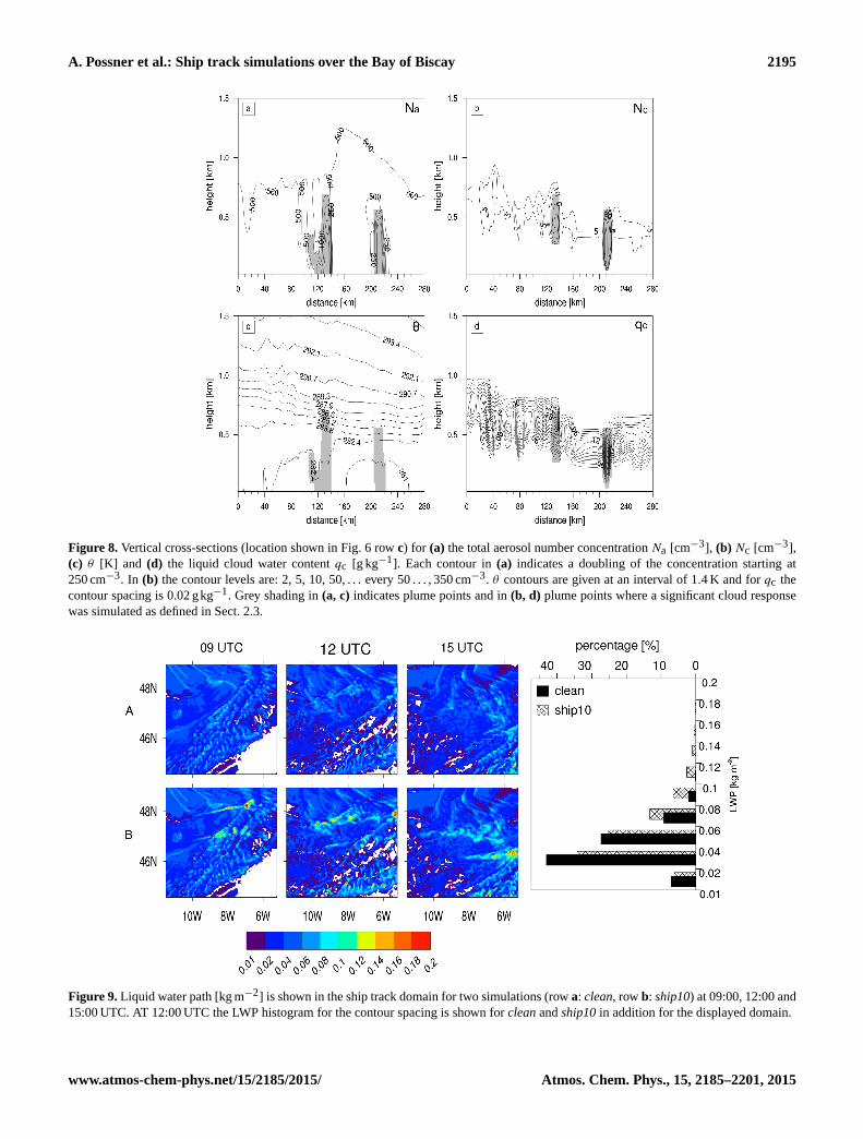
Figure 8. Vertical cross-sections (location shown in Fig. 6 row c) for (a) the total aerosol number concentration Na [cm−3], (b) Nc [cm−3],

(c) θ [K] and (d) the liquid cloud water content qc [g kg−1]. Each contour in (a) indicates a doubling of the concentration starting at

250 cm−3. In (b) the contour levels are: 2, 5, 10, 50, . . . every 50 . . . , 350 cm−3. θ contours are given at an interval of 1.4 K and for qc the

contour spacing is 0.02 gkg−1. Grey shading in (a, c) indicates plume points and in (b, d) plume points where a significant cloud response

was simulated as defined in Sect. 2.3.

Figure 9. Liquid water path [kg m−2] is shown in the ship track domain for two simulations (row a: clean, row b: ship10) at 09:00, 12:00 and

15:00 UTC. AT 12:00 UTC the LWP histogram for the contour spacing is shown for clean and ship10 in addition for the displayed domain.

www.atmos-chem-phys.net/15/2185/2015/ Atmos. Chem. Phys., 15, 2185–2201, 2015

2196 A. Possner et al.: Ship track simulations over the Bay of Biscay

Figure 10. (a) Percentage of ship plume points of significant cloud

response determined as in Fig. 7, where at least a 50 % liquid water

path (LWP) increase was detected. Given a 50 % LWP increase in

at least 25 % of all plume points, the percentage of plume perturbed

grid points which additionally displayed a cloud base lowering was

computed and is shown in (b). A cloud base lowering is diagnosed

for any change greater than 0 m. Note that a cloud base lifting was

not detected at any point.

The observed increase in cloud droplet number concentration

ranges between 40 cm−3 (Hobbs et al., 2000) and 800 cm−3

(McComiskey et al., 2009), though most observed cloud

droplet number concentrations lie within a narrower range

of 40 to 200 cm−3 (Ferek et al., 1998; Hobbs et al., 2000;

Hudson et al., 2000; Durkee et al., 2000).

Similarly the in situ observations of cloud effective radii

measured in ship tracks ranged between 6 and 15 µm. This is

almost identical to the range spanned by P25 and P75 in all

simulations. Although these values were obtained for a range

of environmental conditions which are not necessarily simi-

lar to the environmental conditions of this case study, these

measurements provide a basis to demonstrate the realism of

our simulated cloud response.

In line with the increase in Nc, and the decrease of Reff

(Fig. 7), τ increases within the plume regions. In the ship10,

ship10A and ship10_V5 simulations the response in τ varies

between 6 to 10 at the track edges and 12 to 24 within the

track centres. Within the ship simulation the response in τ is

considerably weaker, following the considerably smaller per-

turbations to Nc and Reff, at both 09:00 and 12:00 UTC. An

increase in optical thickness of 8 to 10 was simulated within

the considerably smaller plume areas. A slightly stronger re-

sponse was simulated at 12:00 UTC in ship10_V20, where

the increase in τ ranges between 8 to 14 within the plume

regions.

Due to the significant increase of cloud optical thickness

within the ship track regions, the top of the atmosphere

(TOA) shortwave (SW) cloud radiative effect (CRE), de-

fined as the difference between all-sky outgoing SW and

clear-sky outgoing SW radiation at TOA, was changed. Av-

eraged over the entire ship track domain, the TOA SW CRE

(Fig. 7c) increased in magnitude by 19 % in ship10, ship10A

and ship10_V5. The stronger cooling of the clouds at the

TOA is solely due to changes within the ship tracks them-

selves, which cover at most 6 % of the domain area, while

the background TOA SW CRE variations were no larger than

5 Wm−2 (∼ 3 %) at any given time.

3.4 Interplay between micro- and macrophysics

In confined regions of the simulated ship tracks, the changes

in microphysical properties were found to produce localised

changes of macrophysical entities, such as cloud extent and

in-cloud liquid water content qc. As is shown in Fig. 8,

regions of increased Nc due to the ship exhaust aerosol

were found to coincide with regions of increased qc. The

localised increase of qc is caused by the suppression of

rain formation, since the influx of activated aerosol led to

a significant decrease of cloud droplet size. Within the ship

track domain, the stratocumulus deck is lightly precipitating

with almost all precipitation evaporating before reaching the

surface, thereby moistening the subcloud layer. Starting at

04:00 UTC, the rain water content within the ship track is re-

duced. At 09:00 UTC, the mean rain water content in ship10

within the ship track is reduced in the mean by 45 % and by

38 % at 12:00 UTC.

The resulting increase of liquid water path LWP is not only

seen for the particular cross-section shown, but in several

confined regions of the ship tracks (Fig. 9). The background

LWP ranges between 0.02 and 0.08 kgm−2 and is found to

remain constant throughout the day. Within the ship10 sim-

ulation, the LWP is increased to 0.12 or even 0.16 kgm−2

in ship track regions (Fig. 9), which corresponds to almost a

doubling of the LWP as compared to the background.

Changes in cloud liquid water content and cloud depth due

to increased aerosol concentrations have been shown to affect

cloud life time (Albrecht, 1989). Whether the cloud life time

is increased or decreased depends fundamentally on the ef-

fect of drizzle suppression on the entrainment rate and the hu-

midity in the free troposphere (Stevens et al., 1998). In gen-

eral, precipitation acts to stabilise the boundary layer. In the

case of a collapsed boundary layer such as the one analysed

in this study, where cloud droplet number concentrations and

accumulation size aerosol concentrations are extremely low,

entrainment rates are believed to be small due to the weak

radiative cloud top cooling generated by the optically thin

clouds. Therefore, decreases in precipitation combined with

a re-establishment of CCN have been shown to increase en-

trainment and lead to a re-growth of the previously collapsed

boundary layer. However, entrainment rate parameterisations

in most global and regional climate models are inadequate to

capture such effects. During this case study we are not able

to study possible effects of the ship exhaust on the PBL top

as this process was found to occur on a typical timescale of

the order of days (e.g. Berner et al., 2013). Due to advection

of the air masses into regions of changed environmental con-

ditions the impact of the ship exhaust on the stratiform cloud

deck could only be studied for about 12 h.

Atmos. Chem. Phys., 15, 2185–2201, 2015 www.atmos-chem-phys.net/15/2185/2015/

A. Possner et al.: Ship track simulations over the Bay of Biscay 2197

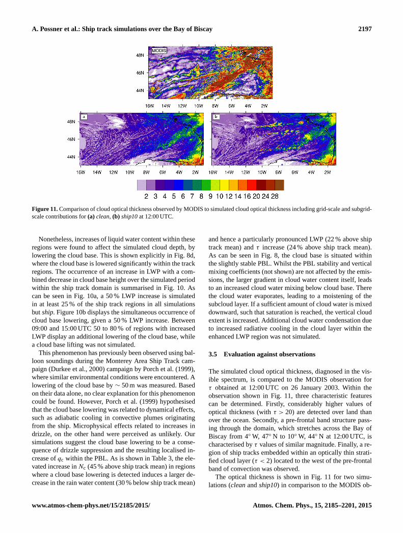
Figure 11. Comparison of cloud optical thickness observed by MODIS to simulated cloud optical thickness including grid-scale and subgrid-

scale contributions for (a) clean, (b) ship10 at 12:00 UTC.

Nonetheless, increases of liquid water content within these

regions were found to affect the simulated cloud depth, by

lowering the cloud base. This is shown explicitly in Fig. 8d,

where the cloud base is lowered significantly within the track

regions. The occurrence of an increase in LWP with a com-

bined decrease in cloud base height over the simulated period

within the ship track domain is summarised in Fig. 10. As

can be seen in Fig. 10a, a 50 % LWP increase is simulated

in at least 25 % of the ship track regions in all simulations

but ship. Figure 10b displays the simultaneous occurrence of

cloud base lowering, given a 50 % LWP increase. Between

09:00 and 15:00 UTC 50 to 80 % of regions with increased

LWP display an additional lowering of the cloud base, while

a cloud base lifting was not simulated.

This phenomenon has previously been observed using bal-

loon soundings during the Monterey Area Ship Track cam-

paign (Durkee et al., 2000) campaign by Porch et al. (1999),

where similar environmental conditions were encountered. A

lowering of the cloud base by ∼ 50 m was measured. Based

on their data alone, no clear explanation for this phenomenon

could be found. However, Porch et al. (1999) hypothesised

that the cloud base lowering was related to dynamical effects,

such as adiabatic cooling in convective plumes originating

from the ship. Microphysical effects related to increases in

drizzle, on the other hand were perceived as unlikely. Our

simulations suggest the cloud base lowering to be a conse-

quence of drizzle suppression and the resulting localised in-

crease of qc within the PBL. As is shown in Table 3, the ele-

vated increase in Nc (45 % above ship track mean) in regions

where a cloud base lowering is detected induces a larger de-

crease in the rain water content (30 % below ship track mean)

and hence a particularly pronounced LWP (22 % above ship

track mean) and τ increase (24 % above ship track mean).

As can be seen in Fig. 8, the cloud base is situated within

the slightly stable PBL. Whilst the PBL stability and vertical

mixing coefficients (not shown) are not affected by the emis-

sions, the larger gradient in cloud water content itself, leads

to an increased cloud water mixing below cloud base. There

the cloud water evaporates, leading to a moistening of the

subcloud layer. If a sufficient amount of cloud water is mixed

downward, such that saturation is reached, the vertical cloud

extent is increased. Additional cloud water condensation due

to increased radiative cooling in the cloud layer within the

enhanced LWP region was not simulated.

3.5 Evaluation against observations

The simulated cloud optical thickness, diagnosed in the vis-

ible spectrum, is compared to the MODIS observation for

τ obtained at 12:00 UTC on 26 January 2003. Within the

observation shown in Fig. 11, three characteristic features

can be determined. Firstly, considerably higher values of

optical thickness (with τ > 20) are detected over land than

over the ocean. Secondly, a pre-frontal band structure pass-

ing through the domain, which stretches across the Bay of

Biscay from 4◦W, 47◦ N to 10◦W, 44◦ N at 12:00 UTC, is

characterised by τ values of similar magnitude. Finally, a re-

gion of ship tracks embedded within an optically thin strati-

fied cloud layer (τ < 2) located to the west of the pre-frontal

band of convection was observed.

The optical thickness is shown in Fig. 11 for two simu-

lations (clean and ship10) in comparison to the MODIS ob-

www.atmos-chem-phys.net/15/2185/2015/ Atmos. Chem. Phys., 15, 2185–2201, 2015

2198 A. Possner et al.: Ship track simulations over the Bay of Biscay

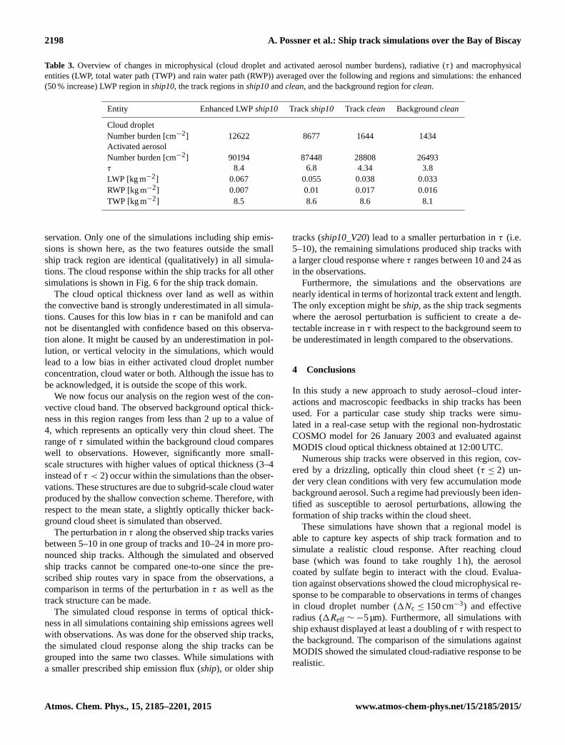
Table 3. Overview of changes in microphysical (cloud droplet and activated aerosol number burdens), radiative (τ ) and macrophysical

entities (LWP, total water path (TWP) and rain water path (RWP)) averaged over the following and regions and simulations: the enhanced

(50 % increase) LWP region in ship10, the track regions in ship10 and clean, and the background region for clean.

Entity Enhanced LWP ship10 Track ship10 Track clean Background clean

Cloud droplet

Number burden [cm−2] 12622 8677 1644 1434

Activated aerosol

Number burden [cm−2] 90194 87448 28808 26493

τ 8.4 6.8 4.34 3.8

LWP [kg m−2] 0.067 0.055 0.038 0.033

RWP [kg m−2] 0.007 0.01 0.017 0.016

TWP [kg m−2] 8.5 8.6 8.6 8.1

servation. Only one of the simulations including ship emis-

sions is shown here, as the two features outside the small

ship track region are identical (qualitatively) in all simula-

tions. The cloud response within the ship tracks for all other

simulations is shown in Fig. 6 for the ship track domain.

The cloud optical thickness over land as well as within

the convective band is strongly underestimated in all simula-

tions. Causes for this low bias in τ can be manifold and can

not be disentangled with confidence based on this observa-

tion alone. It might be caused by an underestimation in pol-

lution, or vertical velocity in the simulations, which would

lead to a low bias in either activated cloud droplet number

concentration, cloud water or both. Although the issue has to

be acknowledged, it is outside the scope of this work.

We now focus our analysis on the region west of the con-

vective cloud band. The observed background optical thick-

ness in this region ranges from less than 2 up to a value of

4, which represents an optically very thin cloud sheet. The

range of τ simulated within the background cloud compares

well to observations. However, significantly more small-

scale structures with higher values of optical thickness (3–4

instead of τ < 2) occur within the simulations than the obser-

vations. These structures are due to subgrid-scale cloud water

produced by the shallow convection scheme. Therefore, with

respect to the mean state, a slightly optically thicker back-

ground cloud sheet is simulated than observed.

The perturbation in τ along the observed ship tracks varies

between 5–10 in one group of tracks and 10–24 in more pro-

nounced ship tracks. Although the simulated and observed

ship tracks cannot be compared one-to-one since the pre-

scribed ship routes vary in space from the observations, a

comparison in terms of the perturbation in τ as well as the

track structure can be made.

The simulated cloud response in terms of optical thick-

ness in all simulations containing ship emissions agrees well

with observations. As was done for the observed ship tracks,

the simulated cloud response along the ship tracks can be

grouped into the same two classes. While simulations with

a smaller prescribed ship emission flux (ship), or older ship

tracks (ship10_V20) lead to a smaller perturbation in τ (i.e.

5–10), the remaining simulations produced ship tracks with

a larger cloud response where τ ranges between 10 and 24 as

in the observations.

Furthermore, the simulations and the observations are

nearly identical in terms of horizontal track extent and length.

The only exception might be ship, as the ship track segments

where the aerosol perturbation is sufficient to create a de-

tectable increase in τ with respect to the background seem to

be underestimated in length compared to the observations.

4 Conclusions

In this study a new approach to study aerosol–cloud inter-

actions and macroscopic feedbacks in ship tracks has been

used. For a particular case study ship tracks were simu-

lated in a real-case setup with the regional non-hydrostatic

COSMO model for 26 January 2003 and evaluated against

MODIS cloud optical thickness obtained at 12:00 UTC.

Numerous ship tracks were observed in this region, cov-

ered by a drizzling, optically thin cloud sheet (τ ≤ 2) un-

der very clean conditions with very few accumulation mode

background aerosol. Such a regime had previously been iden-

tified as susceptible to aerosol perturbations, allowing the

formation of ship tracks within the cloud sheet.

These simulations have shown that a regional model is

able to capture key aspects of ship track formation and to

simulate a realistic cloud response. After reaching cloud

base (which was found to take roughly 1 h), the aerosol

coated by sulfate begin to interact with the cloud. Evalua-

tion against observations showed the cloud microphysical re-

sponse to be comparable to observations in terms of changes

in cloud droplet number (1Nc ≤ 150 cm−3) and effective

radius (1Reff ∼−5µm). Furthermore, all simulations with

ship exhaust displayed at least a doubling of τ with respect to

the background. The comparison of the simulations against

MODIS showed the simulated cloud-radiative response to be

realistic.

Atmos. Chem. Phys., 15, 2185–2201, 2015 www.atmos-chem-phys.net/15/2185/2015/

A. Possner et al.: Ship track simulations over the Bay of Biscay 2199

The resulting cloud radiative effect is largely determined

by the change in CCN due to the ship emissions. The CCN

concentration in turn is intrinsically linked to the aerosol per-

turbation within the soluble Aitken and accumulation modes.

These simulations showed the aerosol size distribution per-

turbation to be very sensitive to the emission flux and size. A

scaling of the emission mass flux by a factor of 10 had to be

applied to reproduce observed aerosol size distributions near

the source, which defines the size distribution within the en-

tire exhaust plume and hence the potential CCN perturbation

by ship emissions. While some uncertainty remains with the

observations, the dilution of literature ship emissions onto

the grid scale, which provides a grid-scale mean perturba-

tion to the system, may lead to a significant underestimation

of their potential effects. However, the performed scaling of

the emission fluxes leads to a considerable overestimation of

peak concentrations in ship10. In this manner the simulations

highlight the issues tied to analysing effects of a rapidly mi-

crophysically processed point-source aerosol emission with

parameterisations based on grid-scale mean fields operating

at discretised time steps. In order to determine the magnitude

and sensitivity of the emission dilution effect, simulations for

a range of computational resolutions, including LES resolu-

tion, would be highly desirable.

Although global studies are based on fundamentally dif-

ferent ship emission inventories than those used in this study,

they are still restricted to area-weighted emission fluxes

over grid box sizes of O(100) km. Furthermore, given atmo-

spheric residence times of SO4, BC and OC of several days to

a week, biases in the predicted aerosol number perturbation

due to ship emissions could introduce significant uncertain-

ties in radiative forcing estimates. Indeed it has been shown

in global simulations, based on the same aerosol microphys-

ical parameterisation, that a tenfold upscaling of the emis-

sion inventories did induce significant changes in microphys-

ical and macrophysical quantities surpassing the background

noise (Peters et al., 2014).

Besides the microphysical and radiative response, changes

in cloud structure and liquid water content were simulated.

The liquid water content was found to have increased by

50 % in at least 25 % of the ship tracks, which coincided

with a cloud base lowering in over 70 % at the early onset

of ship track formation. By vertical mixing of cloud water

within the boundary layer and evaporation below cloud base

the condensation level was lowered in the simulations.

On the whole, these simulations give confidence in the re-

alism of a multitude of simulated processes occurring pre-

dominantly on the parameterised scale. To further constrain

parameterisations which are widely used in regional and

global models using this kind of approach, a more compre-

hensive data set would be required. In order to attribute bi-

ases to particular parameterisations (turbulence, cloud and

aerosol microphysics, radiation, shallow convection, etc.) si-

multaneous observations of the boundary layer and turbulent

structure, ship emission, background aerosol concentrations

and composition as well as cloud property measurements in

and around the ship track would be needed, most of which

were obtained during the Monterey Area Ship-Track cam-

paign (e.g. Noone et al., 2000).

Acknowledgements. We wish to thank the Swiss National Super-

computing Centre (CSCS) for providing Cray XC30 platforms for

the simulations of this study. Furthermore, we thank the COSMO

consortium for code access, the German weather service (DWD)

and MeteoSwiss for code maintenance and setup, as well as C2SM

for source code support. In particular we would like to thank Dani

Lüthi for his help on data handling and technical support.

Edited by: J. Quaas

References

Abdul-Razzak, H. and Ghan, S. J.: A parameterization of aerosol

activation 2. Multiple aerosol types, J. Geophys. Res., 105, 6837–

6844, 2000.

Ackerman, A. S., Toon, O. B., and Hobbs, P. V.: Dissipation of ma-

rine stratiform clouds and collapse of the marine boundary layer

due to the depletion of cloud condensation nuclei by clouds, Sci-

ence, 262, 226–229, 1993.

Albrecht, B. A.: Aerosols, cloud microphysics, and fractional

cloudiness, Science, 245, 1227–1230, 1989.

Berner, A. H., Bretherton, C. S., Wood, R., and Muhlbauer, A.:

Marine boundary layer cloud regimes and POC formation in a

CRM coupled to a bulk aerosol scheme, Atmos. Chem. Phys.,

13, 12549–12572, doi:10.5194/acp-13-12549-2013, 2013.

Bodas-Salcedo, A., Webb, M. J., Bony, S., Chepfer, H.,

Dufresne, J.-L., Klein, S. A., Zhang, Y., Marchand, R.,

Haynes, J. M., Pincus, R., and John, V. O.: COSP: A satellite sim-

ulation software for model assessment, B. Am. Meteorol. Soc.,

92, 1023–1043, 2011.

Bott, A.: A positive definite advection scheme obtained by nonlin-

ear renormalization of the advective fluxes, Mon. Weather Rev.,

117, 1006–1015, 1989.

Chen, Y.-C., Christensen, M. W., Xue, L., Sorooshian, A.,

Stephens, G. L., Rasmussen, R. M., and Seinfeld, J. H.: Occur-

rence of lower cloud albedo in ship tracks, Atmos. Chem. Phys.,

12, 8223–8235, doi:10.5194/acp-12-8223-2012, 2012.

Christensen, M. and Stephens, G.: Microphysical and macrophys-

ical responses of marine stratocumulus polluted by underlying

ships: 2. Impacts of haze on precipitating clouds, J. Geophys.

Res., 116, D11203, doi:10.1029/2010JD014638, 2011.

Christensen, M. and Stephens, G.: Microphysical and macrophys-

ical responses of marine stratocumulus polluted by underly-

ing ships: evidence of cloud deepening, J. Geophys. Res., 117,

D03201, doi:10.1029/2011JD017125, 2012.

Coakley, J. A., Bernstein, R. L., and Durkee, P. A.: Effect of ship

track effluents on cloud reflectivity, Science, 237, 1020–1022,

1987.

Corbett, J. J.: Updated emissions from ocean shipping, J. Geophys.

Res., 108, 4650, doi:10.1029/2003JD003751, 2003.

Dee, D. P., Uppala, S. M., Simmons, A. J., et al.: The ERA-Interim

reanalysis: configuration and performance of the data assimila-

tion system, Q. J. Roy. Meteor. Soc., 137, 553–597, 2011.

www.atmos-chem-phys.net/15/2185/2015/ Atmos. Chem. Phys., 15, 2185–2201, 2015

2200 A. Possner et al.: Ship track simulations over the Bay of Biscay

Durkee, P. A., Noone, K. J., and Bluth, R. T.: The Monterey Area

Ship Track Experiment, J. Atmos. Sci., 57, 2523–2541, 2000.

Ferek, R. F., Hegg, D. A., and Hobbs, P. V.: Measurements of ship-

induced tracks in clouds off the Washington coast, J. Geophys.

Res., 103, 23199–23206, doi:10.1029/98JD02121, 1998.

Foerstner, J. and Doms, G.: Runge–Kutta Time Integration and

High-Order Spatial Discretization of Advection – A New Dy-

namical Core for the LMK, COSMO, COSMO Newsletter,

No. 4, 168–176, 2004.

Folini, D. and Wild, M.: Aerosol emissions and dim-

ming/brightening in Europe: sensitivity studies with

ECHAM5-HAM, J. Geophys. Res., 116, D21104,

doi:10.1029/2011JD016227, 2011.

Goren, T. and Rosenfeld, D.: Satellite observations of ship emis-

sions induced transitions from broken to closed cell marine stra-

tocumulus over large areas, J. Geophys. Res., 117, D17206,

doi:10.1029/2012JD017981, 2012.

Guelle, W., Schulz, M., Balkanski, Y., and Dentener, F.: Influence

of source formulation on modeling the atmospheric global distri-

bution of sea salt aerosol, J. Geophys. Res., 106, 27509–27524,

doi:10.1029/2001JD900249, 2001.

Hobbs, P. V., Garrett, T. J., Ferek, R. J., Strader, S. R., Hegg, D. A.,

Frick, G. M., Hoppel, W. A., Gasparovic, R. F., Russel, L. M.,

Johnson, D. W., O’Dowd, C., Durkee, P. A., Nielsen, K. E., and

Innis, G.: Emissions from ships with respect to their effects on

clouds, J. Atmos. Sci., 57, 2570–2590, 2000.

Hu, Y. X. and Stamnes, K.: An accurate parameterization of the

radiative properties of water clouds suitable for use in climate

models, J. Climate, 6, 728–742, 1993.

Hudson, J., Garrett, T. J., Hobbs, P. V., and Strader, S. R.: Cloud

condensation nuclei and ship tracks, J. Atmos. Sci., 57, 2696–

2706, 2000.

Kazil, J., Wang, H., Feingold, G., Clarke, A. D., Snider, J. R.,

and Bandy, A. R.: Modeling chemical and aerosol processes in

the transition from closed to open cells during VOCALS-REx,

Atmos. Chem. Phys., 11, 7491–7514, doi:10.5194/acp-11-7491-

2011, 2011.

King, M. D., Tsay, S.-C., Platnick, S. E., Wang, M., and Liou, K.-

N.: Cloud Retrieval Algorithms for MODIS: Optical Thickness,

Effective Particle Radius and Thermodynamic Phase, NASA,

No. ATBD-MOD-05, 1998.

Kinne, S., Schulz, M., Textor, C., Guibert, S., Balkanski, Y.,

Bauer, S. E., Berntsen, T., Berglen, T. F., Boucher, O., Chin, M.,

Collins, W., Dentener, F., Diehl, T., Easter, R., Feichter, J.,

Fillmore, D., Ghan, S., Ginoux, P., Gong, S., Grini, A., Hen-

dricks, J., Herzog, M., Horowitz, L., Isaksen, I., Iversen, T.,

Kirkevåg, A., Kloster, S., Koch, D., Kristjansson, J. E., Krol, M.,

Lauer, A., Lamarque, J. F., Lesins, G., Liu, X., Lohmann, U.,

Montanaro, V., Myhre, G., Penner, J., Pitari, G., Reddy, S., Se-

land, O., Stier, P., Takemura, T., and Tie, X.: An AeroCom ini-

tial assessment – optical properties in aerosol component mod-

ules of global models, Atmos. Chem. Phys., 6, 1815–1834,

doi:10.5194/acp-6-1815-2006, 2006.

Lack, D. A., Corbett, J. J., Onasch, T., Lerner, B., Massoli, P.,

Quinn, P. K., Bates, T. S., Covert, D. S., Coffman, D.,

Sierau, B., Herndon, S., Allan, J., Baynard, T., Lovejoy, E., Rav-

ishankara, A. R., and Williams, E.: Particulate emissions from

commercial shipping: chemical, physical and optical properties,

J. Geophys. Res., 114, D00F04, doi:10.1029/2008JD011300,

2009.

Lauer, A., Eyring, V., Hendricks, J., Jöckel, P., and Lohmann, U.:

Global model simulations of the impact of ocean-going ships on

aerosols, clouds, and the radiation budget, Atmos. Chem. Phys.,

7, 5061–5079, doi:10.5194/acp-7-5061-2007, 2007.

Lin, H. and Leaitch, W. R.: Development of an in-cloud aerosol ac-

tivation parameterization for climate modeling, in: Proc. WMO

Workshop on Measurements of Cloud Properties for Forecasts of

Weather and Climate, edited by: Baumgardner, D., and Raga, G.,

Mexico City, Mexico, 23–27 June 1997, 328–335, 1997.

Lohmann, U.: Possible aerosol effects on ice clouds via contact nu-

cleation, J. Atmos. Sci., 59, 647–656, 2002.

Lohmann U. and Stier P. and Hoose C. and Ferrachat S. and

Kloster S. and Roeckner E., and Zhang J.: Cloud micro-

physics and aerosol indirect effects in the global climate model

ECHAM5-HAM, Atmos. Chem. Phys., 7, 3425–3446, 2007,

http://www.atmos-chem-phys.net/7/3425/2007/.

Lund, M. T., Eyring, V., Fuglestvedt, J., Hendricks, J., Lauer, A.,

Lee, D., and Righi, M.: Global-mean temperature change from

shipping toward 2050: improved representation of the indirect

aerosol effect in simple climate models, Environ. Sci. Technol.,

46, 8868–8877, doi:10.1021/es301166e, 2012.

McComiskey, A., Feingold, G., Frisch, A. S., Turner, D. D.,

Miller, M. A., Chiu, J. C., Min, Q., and Ogren, J. A.: An as-

sessment of aerosol-cloud interactions in marine stratus clouds

based on surface remote sensing, J. Geophys. Res., 114, D09203,

doi:10.1029/2008JD011006, 2009.

Moldanová, J., Fridell, E., Popovicheva, O., Demirdjian, B.,

Tishkova, V., Faccinetto, A., and Focsa, C.: Characterisation of

particulate matter and gaseous emissions from a large ship diesel

engine, Atmos. Environ., 43, 2632–2641, 2009.

Murphy, S. M., Agrawal, H., Sorooshian, A., Padró, L. T., Gates, H.,

Hersey, S., Welch, W. A., Jung, H., Miller, J. W., D. R.

Cocker III, A. N., Jonsson, H. H., Flagan, R. C., and Seinfeld, J.:

Comprehensive simultaneous shipboard and airborne characteri-

zation of exhaust from a modern container ship at sea, Environ.

Sci. Technol., 43, 4626–4640 doi:10.1021/es802413j, 2009.

Myhre, G., Shindell, D., Bréon, F.-M., et al.: Climate Change 2013:

The Physical Science Basis. Contribution of Working Group I to

the Fifth Assessment Report of the Intergovernmental Panel on

Climate Change, Cambridge University Press, Cambridge, UK

and New York, USA, 2013.

Nam, C., Bony, S., Dufresne, J.-L., and Chepfer, H.: The “too few,

too bright” tropical low-cloud problem in CMIP5 models, Geo-

phys. Res. Lett., 39, L21801, doi:10.1029/2012GL053421, 2012.

Nenes, A. and Seinfeld, J. H.: Parameterization of cloud droplet

formation in global climate models, J. Geophys. Res., 108, 4415,

doi:10.1029/2002JD002911, 2003.

Noone, K. J., Johnson, D. W., Taylor, J. P., Ferek, R. J., Gar-

ret, T., Hobbs, P. V., Durkee, P. A., Nielson, K., Platnick, S.,

King, M. D., Öström, E., O’Dowd, C. D., Smith, M. H., Rus-

sel, L. M., Flagan, R. C., Seinfeld, J. H., DeBock, L., van

Grieken, R., Hudson, J. G., Brooks, I. M., Gasparovic, R. F., and

Pockalny, R. A.: A case study of ship track formation in a pol-

luted boundary layer, J. Atmos. Sci., 57, 2748–2764, 2000.

Nozawa T. and Nagashima T. and Ogura T. and Yokohata T. and

Okada N. and Shiogama M.: Climate Change Simulations With

a Coupled Ocean-Atmosphere GCM Called the Model for In-

Atmos. Chem. Phys., 15, 2185–2201, 2015 www.atmos-chem-phys.net/15/2185/2015/

A. Possner et al.: Ship track simulations over the Bay of Biscay 2201

terdisciplinary Research on Climate: MIROC, CGER’s Super-

computer Monogr. Rep. Ser., Vol. 12, 79 pp., Natl. Inst. for En-

viron. Stud., Tsukuba, Jpn., available at: //www.cger.nies.go.jp/

publications/report/i073/I073.pdf, 2007.

Partanen, A. I., Laakso, A., Schmidt, A., Kokkola, H., Kuokka-

nen, T., Pietikäinen, J.-P., Kerminen, V.-M., Lehtinen, K. E. J.,

Laakso, L., and Korhonen, H.: Climate and air quality trade-

offs in altering ship fuel sulfur content, Atmos. Chem. Phys., 13,

12059–12071, doi:10.5194/acp-13-12059-2013, 2013.

Peters, K., Quaas, J., and Graßl, H.: A search for large-scale effects

of ship emissions on clouds and radiation in satellite data, J. Geo-

phys. Res., 116, D24205, doi:10.1029/2011JD016531, 2011.

Peters, K., Stier, P., Quaas, J., and Graßl, H.: Aerosol indirect ef-

fects from shipping emissions: sensitivity studies with the global

aerosol-climate model ECHAM-HAM, Atmos. Chem. Phys., 12,

5985–6007, doi:10.5194/acp-12-5985-2012, 2012.

Peters, K., Quaas, J., Stier, P., and Graßl, H.: Processes limiting

the ermergence of detectable aerosol indirect effects on tropical

warm clouds in global aerosol-climate model and satellite data,

Tellus B, 66, 24054, doi:10.3402/tellusb.v66.24054, 2014.

Petzold, A., Hasselbach, J., Lauer, P., Baumann, R., Franke, K.,

Gurk, C., Schlager, H., and Weingartner, E.: Experimental stud-

ies on particle emissions from cruising ship, their characteris-

tic properties, transformation and atmospheric lifetime in the

marine boundary layer, Atmos. Chem. Phys., 8, 2387–2403,

doi:10.5194/acp-8-2387-2008, 2008.

Platnick, S., King, M. D., Ackermann, S. A., Menzel, W. P.,

Baum, B. A., Riedi, J. C., and Frey, R. A.: The MODIS cloud

products: algorithms and examples from Terra, IEEE T. Geosci.

Remote, 41, 459–473, doi:10.1109/TGRS.2002.808301, 2003.

Porch, W., Borys, R., Durkee, P., Gasparovic, R., Hooper, W., Hind-

man, E., and Nielsen, K.: Observations of ship tracks from ship-

based platforms, J. Appl. Meteorol., 38, 69–81, 1999.

Possner, A., Zubler, E., Fuhrer, O., Lohmann, O., and Schär, C.: A

case study in modeling low-lying inversions and stratocumulus

cloud cover in the Bay of Biscay, Weather Forecast., 29, 289–

304, 2014.

Righi, M., Klinger, C., Eyring, V., Hendricks, J., Lauer, A., and Pet-

zold, A.: Climate impact of biofuels in shipping: global model

studies of the aerosol indirect effect, Environ. Sci. Technol., 45,

3519–3525, 2011.

Ritter, B. and Geleyn, J. F.: A comprehensive radiation scheme for

numerical weather prediction models with potential applications

in climate simulations, Mon. Weather Rev., 120, 303–325, 1992.

Roeckner E. and Stier P. and Feichter J. and Kloster S. and Esch M.

and Fischer-Bruns I.: Impact of carbonaceous aerosol emissions

on regional climate change, 27, 553–571, 2006.

Schreier, M., Mannstein, H., Eyring, V., and Bovensmann, H.:

Global ship track distribution and radiative forcing from

1 year of AATSR data, Geophys. Res. Lett., 34, L17814,

doi:10.1029/2007GL030664, 2007.

Seifert, A. and Beheng, K. D.: A two-moment cloud microphysics

parameterization for mixed-phase clouds. Part 1: Model descrip-

tion, Meteorol. Atmos. Phys., 92, 45–66, 2006.

Stevens, B. and Feingold, G.: Untangling aerosol effects on clouds

and precipitation in a buffered system, Nature, 461, 607–613,

2009.

Stevens, B., Cotton, W. R., Feingold, G., and Moeng, C. H.:

Large-eddy simulations of strongly precipitating, shallow,

stratocumulus-topped boundary layers, J. Atmos. Sci., 55, 3616–

3638, 1998.

Stier, P. and Feichter, J. and Kinne S. and Kloster S. and Vignati E.

and Wilson J. and Ganzeveld L. and Tegen L. and Tegen I. and

Werner M. and Balkanski Y. and Schulz M. and Boucher O.

and Minikin A. and Petzold A.: The aerosol climate model

ECHAM5-HAM, Atmos. Chem. Phys., 5, 1125–1156, 2005,

http://www.atmos-chem-phys.net/5/1125/2005/.

Stier P. and Feichter J. and Roeckner E. and Kloster S. and Esch M.:

The evolution of the global aerosol system in a transient climate

simulation from 1860 to 2100, Atmos. Chem. Phys., 6, 3059–

3076, 2006,

http://www.atmos-chem-phys.net/6/3059/2006/.

Tiedtke, M.: A comprehensive mass flux scheme for cumulus pa-

rameterization in large-scale models, Q. J. Roy. Meteor. Soc.,

117, 1779–1800, 1989.

Twomey, S.: Pollution and planetary albedo, Atmos. Environ., 25,

2435–2442, 1974.

Uppala, S. M., Kallberg, P. W., and Simmons, A. J.: The ERA-40

re-analysis, Q. J. Roy Meteor. Soc., 131, 2961–3012, 2005.

Verzijlbergh, R. A., Jonker, H. J. J., Heus, T., and Vilà-

Guerau de Arellano, J.: Turbulent dispersion in cloud-

topped boundary layers, Atmos. Chem. Phys., 9, 1289–1302,

doi:10.5194/acp-9-1289-2009, 2009.

Vignati, E., Wilson, J., and Stier, P.: M7: An efficient

size-resolved aerosol microphysics module for large-scale

aerosol transport models, J. Geophys. Res., 109, D22202,

doi:10.1029/2003JD004485, 2004.

Vutukuru, S. and Dabdub, D.: Modeling the effects of ship emis-

sions on coastal air quality: a case study of southern California,

Atmos. Environ., 42, 3751–3764, 2008.

Wang, H. and Feingold, G.: Modeling mesoscale cellular struc-

tures and drizzle in marine stratocumulus. Part II: Microphysics

and dynamcis of the boundary region between open and closed

cells, J. Atmos. Sci., 66, 3257–3275, 2009.

Wang, H., Rasch, P. J., and Feingold, G.: Manipulating marine

stratocumulus cloud amount and albedo: a process-modelling

study of aerosol-cloud-precipitation interactions in response to

injection of cloud condensation nuclei, Atmos. Chem. Phys., 11,

4237–4249, doi:10.5194/acp-11-4237-2011, 2011.

Wicker, L. J. and Skamarock, W. C.: Time-splitting methods for

elastic models using forward time schemes, Mon. Weather Rev.,

130, 2088–2097, 2002.

Wood, R.: Review: stratocumulus clouds, Mon. Weather Rev., 140,

2373–2423, 2012.

Wood, R., Bretherton, C. S., Leon, D., Clarke, A. D., Zuidema, P.,

Allen, G., and Coe, H.: An aircraft case study of the spatial

transition from closed to open mesoscale cellular convection

over the Southeast Pacific, Atmos. Chem. Phys., 11, 2341–2370,

doi:10.5194/acp-11-2341-2011, 2011.

Zubler, E., Folini, D., Lohmann, U., Lüthi, D., Mühlbauer, A.,

Pousse-Nottelmann, S., Schär, C., and Wild, M.: Implemen-

tation and evaluation of aerosol and cloud microphysics in

a regional climate model, J. Geophys. Res., 116, D02211,

doi:10.1029/2010JD014572, 2011.

www.atmos-chem-phys.net/15/2185/2015/ Atmos. Chem. Phys., 15, 2185–2201, 2015