Real Estate Equity Derivatives - MIT OpenCourseWare Estate Equity Derivatives A derivative is an...

Real Estate Equity Derivatives

Geltner – Miller 2nd Edition

Chapter 26

Section 26.3Section 26.3

Real Estate DerivativesReal Estate Derivatives

(Index Return Swaps)

Real Estate Equity Derivatives

A derivative is an asset whose value depends completely on the value of another asset (or a combination of assets).e.g., Stock options.

Currently, private equity R.E. derivatives offered are essentially “futures” contracts:• No cash changes hands up front (“notional trade amt.”)

The major products are “swaps”:• e.g., Swap NPI return for a fixed return each quarter.

Products Currently Offered

• NPI Appreciation Swap for Fixed

• NPI Total Return Swap for Fixed

• NPI Property Type Total Return Swap

• Similar products on IPD in U.K.

How Derivatives Work:An Example . . .

• Littleton Fireman’s Fund is a Pension Fund that wants to invest in direct (private) real estate for portfolio diversification

• But Littleton is small: They face high transaction costs and/or low diversification within real estate (few properties: “noise”, “basis risk”); and

• Littleton is worried about lack of private R.E. liquidity (10 year investment?!?...)

• Southern State Teachers is a large pension fund, already invested in real estate.

• Southern finds itself over-invested in R.E. due to “denominator effect” (stock mktdecline puts them over-target in R.E.).

• Southern hates to sell any of their individual properties because they like these properties and they hate to incur the high transactions cost of sale; but

• They need to reduce their exposure to the R.E. asset class in their portfolio.


Both parties can benefit from the NCREIF Appreciation Swap:• Littleton takes the “long” position (swaps fixed return for NPI appreciation return).• Southern takes the “short” position (swaps NPI appreciation return for the fixed return).• Southern pays Littleton (short pays long) the NPI appreciation return (“floating leg”) on the notional trade amount each quarter.• Littleton pays Southern (long pays short) the “fixed leg” (spread) on the notional trade amount each quarter.• Net cash owed is settled at the end of each quarter when the NPI is reported, for duration of swap contract (typically 2-3 years).

Suppose Littleton & Southern agree on a two year contract to trade a “notional”amount of $100 million at the end of 2005, with a “fixed leg” (spread) of 100bps:• No cash changes hands at end of 2005Q4.• Suppose 2006Q1 NPI appreciation return is 2.5%, then:

• Southern owes Littleton (short owes long) .025*$100 = $2,500,000;• Littleton owes Southern (long owes short) .01*$100 = $1,000,000;• They settle net cash flow: Southern pays Littleton $1,500,000.

• Suppose 2006Q2 NPI appreciation return is then negative 1.0%:• Southern owes Littleton -.01*$100 = -$1,000,000 (i.e., Littleton owes Southern $1,000,000);• Littleton still owes Southern another $1,000,000 on the fixed spread (as always);• They settle net cash flow: Littleton pays southern $2,000,000.

• This process continues through 2007Q4.



Portfolio risk impact on Littleton (long position):

• Gains risk effect of $100 million worth of real estate investment;

• Loses risk effect of $100 million worth of riskfree bond investment.

i.e.: They’ve “swapped” $100 million of riskfree bond risk for $100 million of private R.E. risk (because virtually all of the quarterly risk in R.E. investment is in the appreciation return).


Portfolio risk impact on Southern (short position):

• Gains risk effect of $100 million worth of riskfree bonds;

• Loses risk effect of $100 million worth of private R.E. investment (like NPI).

i.e.: They’ve “swapped” $100 million of real estate risk for $100 million of riskfree bond risk (i.e., they’ve eliminated $100 million worth of R.E. risk exposure, again because virtually all of the quarterly risk in R.E. investment is in the appreciation return, and the fixed spread is riskless).


• Littleton (long position) “covers” their exposure to the fixed spread by holding $100 million of riskfree bonds in their portfolio.

• Southern (short position) “covers” their exposure to the floating leg (NPI appreciation return) by holding $100 million of real estate (similar to NCREIF properties) in their portfolio.

How Littleton might have arrived at their $100 million long purchase:• Littleton previously had total portfolio $300 million invested 50%/50% Stocks & Bonds. They want to move to equal shares Stocks, Bonds & Real Estate (for diversification):• First Littleton sells $50 million in Stocks & invests proceeds in bonds, so:• Now Littleton has $100 million in Stocks (= target) and $200 million in bonds (= target + $100 million).• Bond investment over target is invested in riskfree bonds ($100 million to cover fixed spread in R.E. derivative).• Next Littleton buys $100 million long position in R.E. appreciation return swap (requires zero cash investment).• Littleton now effectively has risk exposure like $100 million each in Stocks, Bonds, Real Estate, although actually still owns $200 million in bonds.

Derivatives for Portfolio Balance…

Littleton could accomplish this same result by buying $100 million worth of properties or private R.E. investment funds.However:

• Transaction costs & management fees might be higher than derivative fees.

• Effectively fewer number of properties (even in a fund) would add “noise” and/or “basis risk” compared to derivative that tracks NPI benchmark.

• There might be less liquidity or a longer horizon fixed commitment (less investment flexibility), certainly with direct property investment, possibly with fund investment (depending on type of fund).


Another consideration:

For property returns to be as liquid as derivative returns, property returns must be based on transaction prices.

Derivative returns are based on an appraisal-based index (at least in the case of NPI & IPD), which might have more favorable risk characteristics (due to “smoothing”).(This consideration is better for the long position than the short.)

Derivative Risk vs Property Risk from a Portfolio Perspective

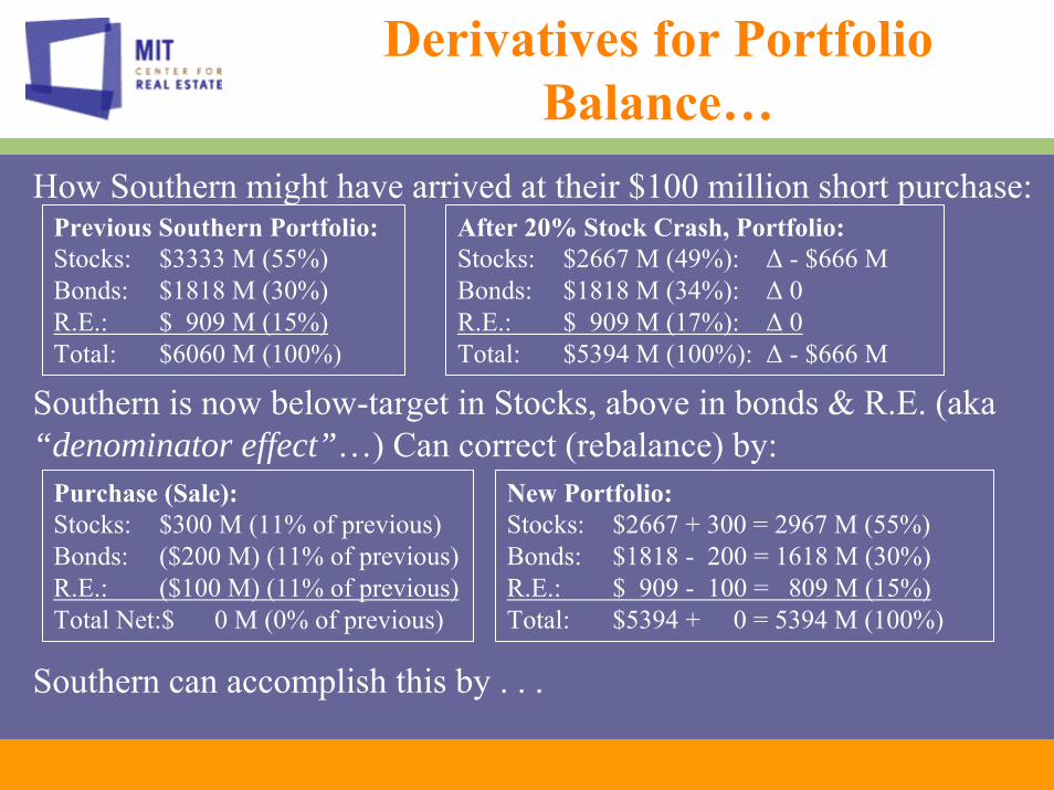
How Southern might have arrived at their $100 million short purchase:Previous Southern Portfolio:Stocks: $3333 M (55%)Bonds: $1818 M (30%)R.E.: $ 909 M (15%)Total: $6060 M (100%)

After 20% Stock Crash, Portfolio:Stocks: $2667 M (49%): Δ - $666 MBonds: $1818 M (34%): Δ 0R.E.: $ 909 M (17%): Δ 0 Total: $5394 M (100%): Δ - $666 M

Southern is now below-target in Stocks, above in bonds & R.E. (aka “denominator effect”…) Can correct (rebalance) by:

Purchase (Sale):Stocks: $300 M (11% of previous)Bonds: ($200 M) (11% of previous) R.E.: ($100 M) (11% of previous) Total Net:$ 0 M (0% of previous)

New Portfolio:Stocks: $2667 + 300 = 2967 M (55%)Bonds: $1818 - 200 = 1618 M (30%)R.E.: $ 909 - 100 = 809 M (15%) Total: $5394 + 0 = 5394 M (100%)

Southern can accomplish this by . . .


Southern can accomplish the above by: • Short $100 M R.E. Derivative (0 cash flow);• Cover R.E. short by “earmarking” $100 M worth of R.E. (like NCREIF) to cover floating leg (R.E. appreciation), thereby reducing R.E. risk exposure to $809 M;• Short $100 riskless bonds (T-Bond futures mkt) (+$100 M cash flow), covered by R.E. Derivative fixed spread, so no impact on portfolio risk exposure;• Sell $200 M bonds (+$200 M cash flow), reducing bond exposure to $1618 M;• Use resulting +$300 M cash flow to purchase stocks, bringing exposure to $2967 M.

Without having to actually sell any properties.

Purchase (Sale):Stocks: $300 M (11% of previous)Bonds: ($200 M) (11% of previous) R.E.: ($100 M) (11% of previous) Total Net:$ 0 M (0% of previous)

New Portfolio:Stocks: $2667 + 300 = 2967 M (55%)Bonds: $1818 - 200 = 1618 M (30%)R.E.: $ 909 - 100 = 809 M (15%) Total: $5394 + 0 = 5394 M (100%)


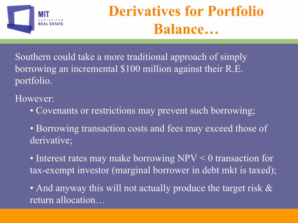
Southern could take a more traditional approach of simply borrowing an incremental $100 million against their R.E. portfolio.

However:• Covenants or restrictions may prevent such borrowing;

• Borrowing transaction costs and fees may exceed those of derivative;

• Interest rates may make borrowing NPV < 0 transaction for tax-exempt investor (marginal borrower in debt mkt is taxed);

• And anyway this will not actually produce the target risk & return allocation…


New Portfolio:Stocks: Use proceeds to buy stock: $2667 + 300 = 2967 M (55%)Bonds: Sell $200 M worth: $1818 - 300 = 1518 M (28%)R.E.: Borrow $100 M like shorting bonds: $ 909 - 0 = 909 M (17%) Total: $5394 + 0 = 5394 M (100%)

The result of simply borrowing $100 million against their R.E. portfolio may reduce the real estate equity on Southern’s books to $809 million, but it increases the leverage of their real estate, thereby retaining the risk and return impact of the full $909 million real estate asset holding in the portfolio.

The borrowing is like “shorting” bonds, thereby negating another $100 million of bond investment in the portfolio risk/return profile, resulting in the following effective portfolio allocation:

The only way to produce the target result without the use of the derivative is by actually selling $100 million worth of Southern’s R.E. properties.


Other Derivative Products

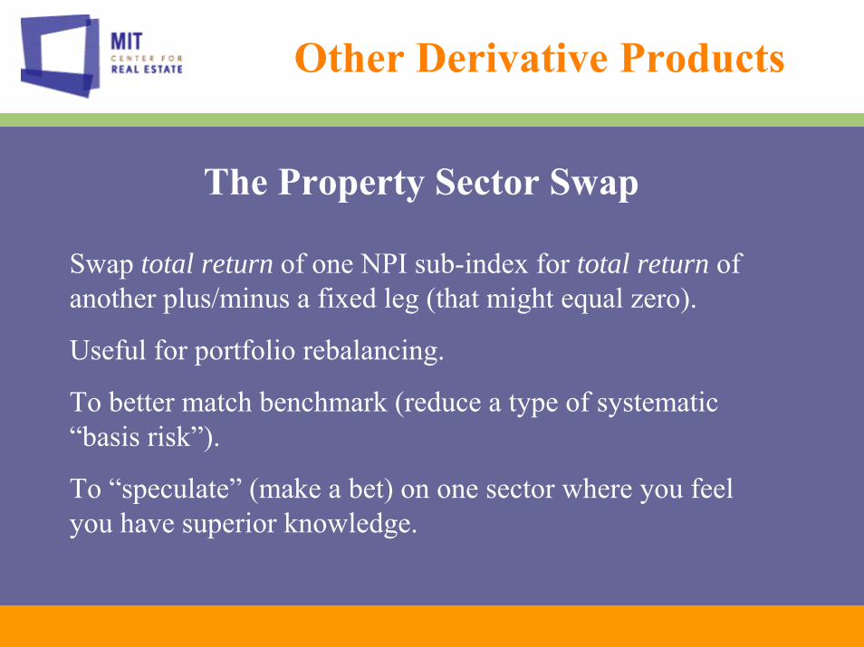
The Property Sector Swap

Swap total return of one NPI sub-index for total return of another plus/minus a fixed leg (that might equal zero).

Useful for portfolio rebalancing.

To better match benchmark (reduce a type of systematic “basis risk”).

To “speculate” (make a bet) on one sector where you feel you have superior knowledge.

Derivatives for Hedging & Speculation…

Previous example showed use of derivative for portfolio balancing or target allocation purposes.

There is another major use for derivatives:

Speculation & Hedging…

Using Derivatives to Make Money in a Down Market…

Suppose you think the real estate market (& NPI) is headed down.

You stand to lose money, even though you are a good real estate asset manager.

You can use the short position in the NPI appreciation or total return future to continue to make money in the down market…

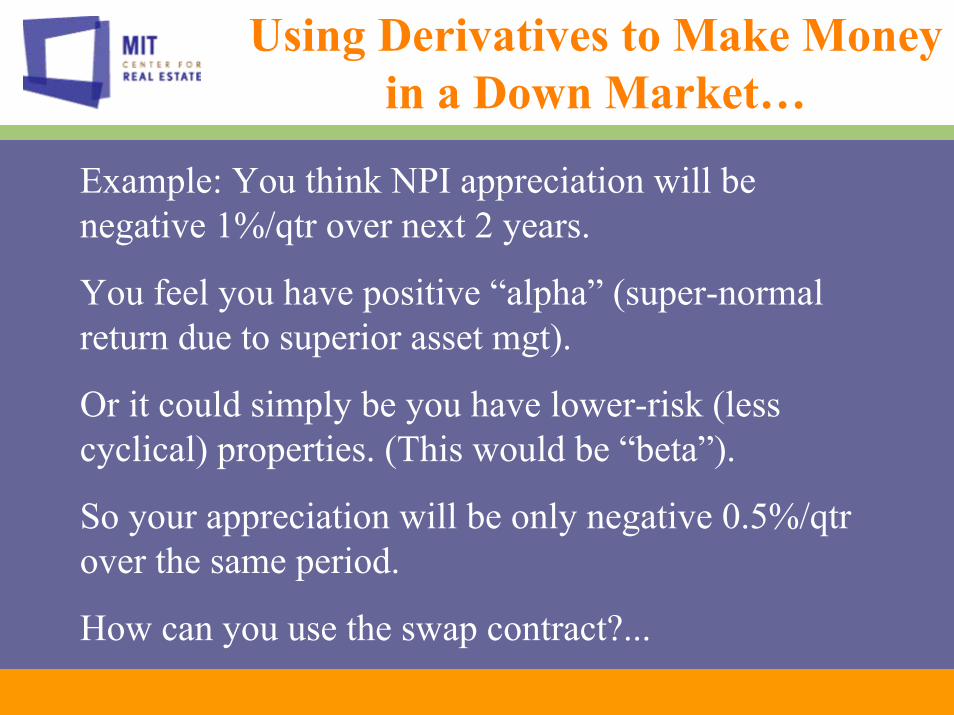
Example: You think NPI appreciation will be negative 1%/qtr over next 2 years.

You feel you have positive “alpha” (super-normal return due to superior asset mgt).

Or it could simply be you have lower-risk (less cyclical) properties. (This would be “beta”).

So your appreciation will be only negative 0.5%/qtr over the same period.

How can you use the swap contract?...


Say you short $100 million of NPI appreciation futures.

If your expectations are born out, you will receive $1 million per qtr from the derivative, plus the fixed spread (which however will probably be negative, hence paid by you).

You lose only about $500,000 per qtr on your property revaluations, leaving you net positive by $500,000 before counting the fixed spread.

If the fixed spread is greater than negative 50 basis-points, you will make money on property appreciation in a down market!

(You of course also still have your properties’ cash yield.)


Even if you don’t have positive “alpha”, shorting the appreciation derivative “hedges” the down side of the real estate market.

Even if you don’t fully cover your property position, you can reduce downside volatility by shorting the appreciation swap.

This is like:

Property Market InsuranceIf you have it when the market is headed down, you will likely “beat the benchmark”, and you will beat the performance of other portfolio managers who haven’t hedged.


Pricing the appreciation swap…

There are two major approaches to analyzing the pricing (or valuation) of the real estate index swap:

• Arbitrage Analysis• Equilibrium Analysis

The two approaches give identical results when the underlying index is always valued at the equilibrium (liquid market) value of its constituent properties.There is also a useful methodology for valuing any swap contract:

• Certainty Equivalence DCF Analysis (CEQ)CEQ valuation is based on equilibrium analysis, but gives results identical to both arbitrage and equilibrium analysis when the underlying index is at equilibrium value.

First consider an “arbitrage analysis” . . .

• Suppose it were possible to hold and efficiently trade long andshort positions in the NPI directly (a so-called “spot market” for the NPI), such that:

• Possible to construct a riskless hedge between the underlying asset and the swap contract:

• Then we could derive a pricing relationship like the classical “Futures-Spot Parity Theorem” . . .

(Aside note: This implies that the index must itself directly reflect equilibrium price and return

expectations.)

We’ll come back to this point later…

Arbitrage Analysis . . .

Let:• Vt = Value level of the underlying appreciation index at end of period t.

• E[y] = Expected income return of the underlying index (assumed constant & riskless).*

• rf = Riskfree interest rate (e.g., LIBOR).

• F = Fixed leg (spread) paid from long to short position (in percent of notional value).

The “price” of the swap contract is given by F, the value of the agreed-upon fixed spread.

F can be derived by arbitrage analysis as follows . . .


Cash Flow Today(t)

Cash Flow End of Qtr(t+1)


Short position in Index +Vt -gt+1Vt - E[y]Vt -gt+2 Vt - E[y]Vt - Vt

Invest risklessly zero-coupon

-Vt / (1+rf)2 0 +Vt

Long position in appreciation swap

0 +gt+1Vt - FVt +gt+2Vt - FVt

Hedge Portfolio = Sum +(1-1/(1+rf)2)Vt -(F+E[y])Vt -(F+E[y])Vt

riskless riskless

Consider a 2-period appreciation swap.Construct a riskless hedge as follows:

Cash Flow Today(t)



Long position in NPI -Vt gt+1Vt + E[y]Vt gt+2 Vt + E[y]Vt + Vt

Borrow risklessly zero-coupon

+Vt / (1+rf)2 0 -Vt

Short position in appreciation swap

0 -gt+1Vt + FVt -gt+2Vt + FVt

Hedge Portfolio = Sum -(1-1/(1+rf)2)Vt (F+E[y])Vt (F+E[y])Vt

riskless riskless

Or on the other side, the riskless hedge for the short…

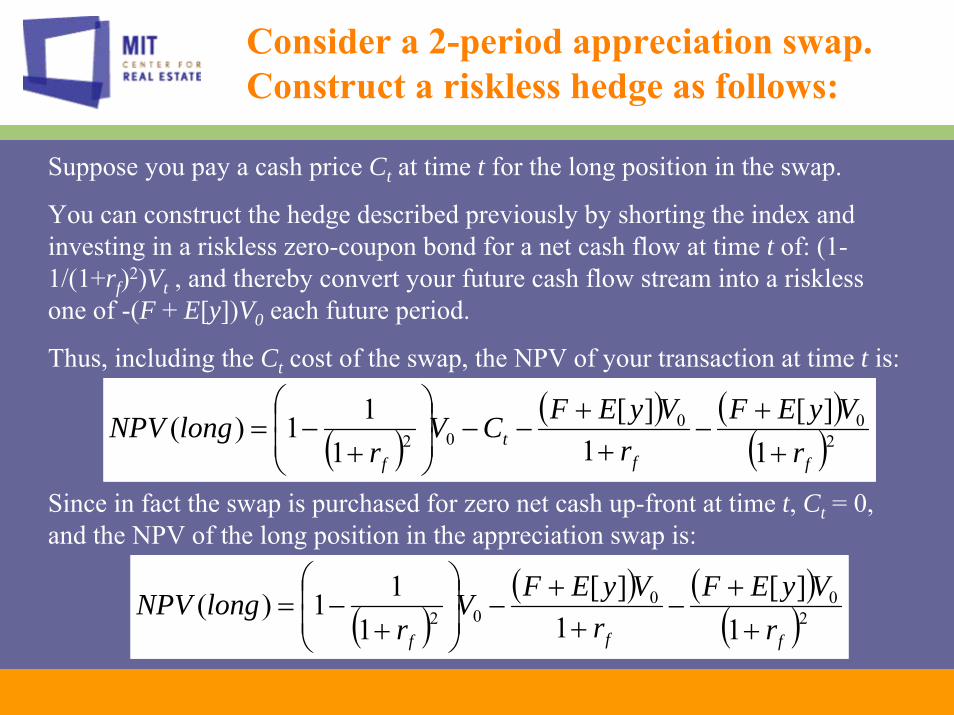
Suppose you pay a cash price Ct at time t for the long position in the swap.

You can construct the hedge described previously by shorting the index and investing in a riskless zero-coupon bond for a net cash flow at time t of: (1-1/(1+rf)2)Vt , and thereby convert your future cash flow stream into a risklessone of -(F + E[y])V0 each future period.

Thus, including the Ct cost of the swap, the NPV of your transaction at time t is:


( )( ) ( )

( )200

02 1][

1][

111)(

fft

f rVyEF

rVyEFCV

rlongNPV

++

−+

+−−⎟

⎟⎠

⎞⎜⎜⎝

⎛

+−=

Since in fact the swap is purchased for zero net cash up-front at time t, Ct = 0, and the NPV of the long position in the appreciation swap is:

( )( ) ( )

( )200

02 1][

1][

111)(

fff rVyEF

rVyEFV

rlongNPV

++

−+

+−⎟

⎟⎠

⎞⎜⎜⎝

⎛

+−=

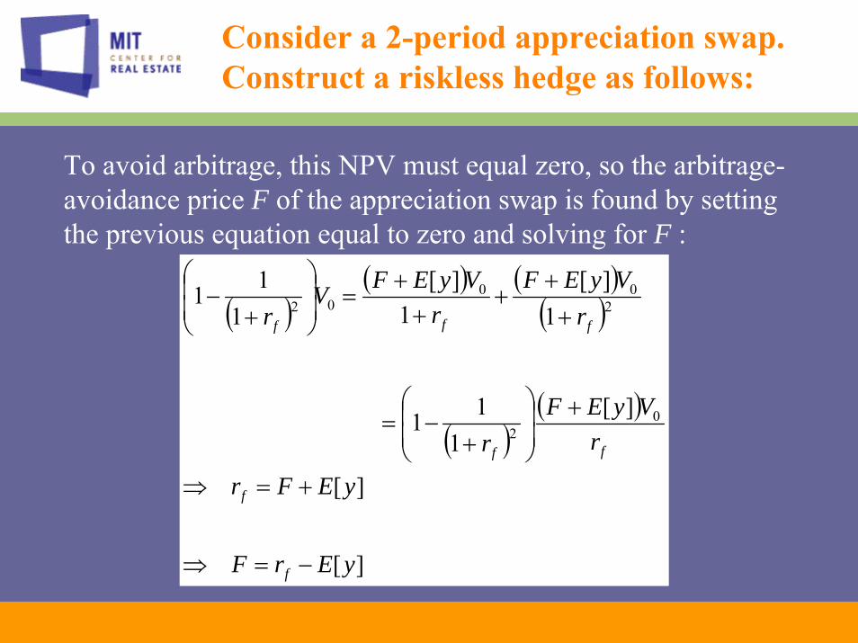
To avoid arbitrage, this NPV must equal zero, so the arbitrage-avoidance price F of the appreciation swap is found by setting the previous equation equal to zero and solving for F :


( )( ) ( )

( )

( )( )

][

][

][1

11

1][

1][

111

02

200

02

yErF

yEFr

rVyEF

r

rVyEF

rVyEFV

r

f

f

ff

fff

−=⇒

+=⇒

+⎟⎟⎠

⎞⎜⎜⎝

⎛

+−=

++

++

+=⎟

⎟⎠

⎞⎜⎜⎝

⎛

+−

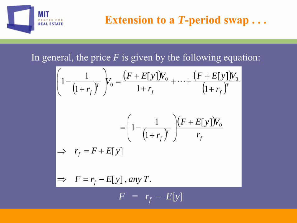
In general, the price F is given by the following equation:

Extension to a T-period swap . . .

F = rf – E[y]

( )( ) ( )

( )

( )( )

.,][

][

][1

11

1][

1][

111

0

000

TanyyErF

yEFr

rVyEF

r

rVyEF

rVyEFV

r

f

f

fT

f

Tff

Tf

−=⇒

+=⇒

+⎟⎟⎠

⎞⎜⎜⎝

⎛

+−=

++

+++

+=⎟

⎟⎠

⎞⎜⎜⎝

⎛

+− L

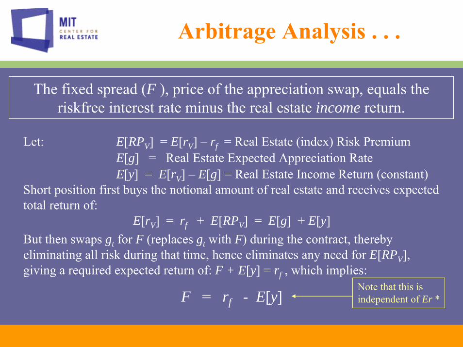
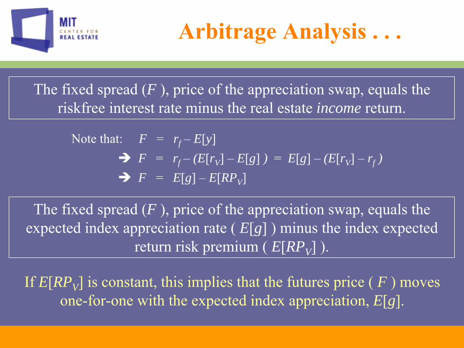
The fixed spread (F ), price of the appreciation swap, equals the riskfree interest rate minus the real estate income return.


Let: E[RPV] = E[rV] – rf = Real Estate (index) Risk PremiumE[g] = Real Estate Expected Appreciation RateE[y] = E[rV] – E[g] = Real Estate Income Return (constant)

Short position first buys the notional amount of real estate and receives expected total return of:

E[rV] = rf + E[RPV] = E[g] + E[y]But then swaps gt for F (replaces gt with F) during the contract, thereby eliminating all risk during that time, hence eliminates any need for E[RPV], giving a required expected return of: F + E[y] = rf , which implies:

F = rf - E[y]Note that this is independent of Er *

The fixed spread (F ), price of the appreciation swap, equals the riskfree interest rate minus the real estate income return.


Note that: F = rf – E[y]F = rf – (E[rV] – E[g] ) = E[g] – (E[rV] – rf )F = E[g] – E[RPV]

The fixed spread (F ), price of the appreciation swap, equals the expected index appreciation rate ( E[g] ) minus the index expected

return risk premium ( E[RPV] ).

If E[RPV] is constant, this implies that the futures price ( F ) moves one-for-one with the expected index appreciation, E[g].


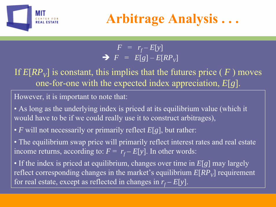
F = rf – E[y]F = E[g] – E[RPV]

If E[RPV] is constant, this implies that the futures price ( F ) moves one-for-one with the expected index appreciation, E[g].

However, it is important to note that:• As long as the underlying index is priced at its equilibrium value (which it would have to be if we could really use it to construct arbitrages),• F will not necessarily or primarily reflect E[g], but rather:• The equilibrium swap price will primarily reflect interest rates and real estate income returns, according to: F = rf – E[y]. In other words:• If the index is priced at equilibrium, changes over time in E[g] may largely reflect corresponding changes in the market’s equilibrium E[RPV] requirement for real estate, except as reflected in changes in rf – E[y].


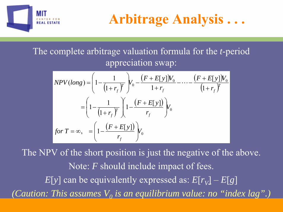
The complete arbitrage valuation formula for the t-period appreciation swap:

( )( ) ( )

( )

( )( )

( )0

0

000

][1,

][11

11

1][

1][

111)(

Vr

yEFTfor

Vr

yEFr

rVyEF

rVyEFV

rlongNPV

f

fT

f

Tff

Tf

⎟⎟⎠

⎞⎜⎜⎝

⎛ +−=∞=

⎟⎟⎠

⎞⎜⎜⎝

⎛ +−⎟

⎟⎠

⎞⎜⎜⎝

⎛

+−=

++

−−+

+−⎟

⎟⎠

⎞⎜⎜⎝

⎛

+−= L

The NPV of the short position is just the negative of the above.Note: F should include impact of fees.

E[y] can be equivalently expressed as: E[rV] – E[g](Caution: This assumes V0 is an equilibrium value: no “index lag”.)

Cash Flow Today(t)



Long position in NPI -Vt rt+1Vt rt+2 Vt + Vt

Borrow risklessly zero-coupon

+Vt / (1+rf)2 0 -Vt

Short position in total return swap

0 -rt+1Vt + FVt -rt+2Vt + FVt

Hedge Portfolio = Sum -(1-1/(1+rf)2)Vt FVt FVt

riskless riskless

For total return swap, the riskless hedge for the short…

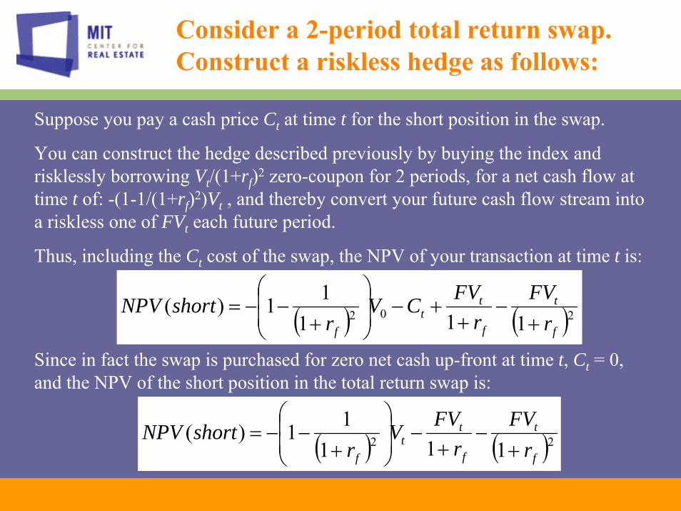
Suppose you pay a cash price Ct at time t for the short position in the swap.

You can construct the hedge described previously by buying the index and risklessly borrowing Vt/(1+rf)2 zero-coupon for 2 periods, for a net cash flow at time t of: -(1-1/(1+rf)2)Vt , and thereby convert your future cash flow stream into a riskless one of FVt each future period.

Thus, including the Ct cost of the swap, the NPV of your transaction at time t is:

Consider a 2-period total return swap.Construct a riskless hedge as follows:

( ) ( )202 11111)(

f

t

f

tt

f rFV

rFVCV

rshortNPV

+−

++−⎟

⎟⎠

⎞⎜⎜⎝

⎛

+−−=

Since in fact the swap is purchased for zero net cash up-front at time t, Ct = 0, and the NPV of the short position in the total return swap is:

( ) ( )22 11111)(

f

t

f

tt

f rFV

rFVV

rshortNPV

+−

+−⎟

⎟⎠

⎞⎜⎜⎝

⎛

+−−=

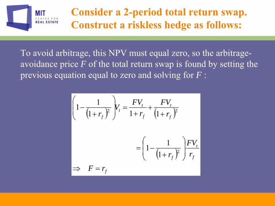
To avoid arbitrage, this NPV must equal zero, so the arbitrage-avoidance price F of the total return swap is found by setting the previous equation equal to zero and solving for F :

Consider a 2-period total return swap.Construct a riskless hedge as follows:

( ) ( )

( )f

f

t

f

f

t

f

tt

f

rF

rFV

r

rFV

rFVV

r

=⇒

⎟⎟⎠

⎞⎜⎜⎝

⎛

+−=

++

+=⎟

⎟⎠

⎞⎜⎜⎝

⎛

+−

2

22

111

11111

Equilibrium Analysis . . .

In real estate we cannot construct the arbitrage, because we cannot directly trade the underlying index.

However, the arbitrage analysis gives a pricing result that equates the expected total return risk premium per unit of risk within and across the relevant asset markets: so-called “linear pricing”…

rfRisk

E[r]

E[RP]

This is a characteristic of equilibrium pricing, which may also be viewed as normative (i.e., “fair” ) pricing.

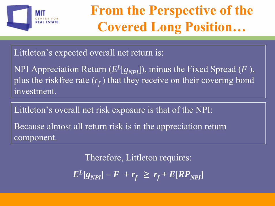
From the Perspective of the Covered Long Position…

Littleton’s expected overall net return is:

NPI Appreciation Return (EL[gNPI]), minus the Fixed Spread (F ), plus the riskfree rate (rf ) that they receive on their covering bond investment.

Littleton’s overall net risk exposure is that of the NPI:

Because almost all return risk is in the appreciation return component.

Therefore, Littleton requires:

EL[gNPI] – F + rf ≥ rf + E[RPNPI]

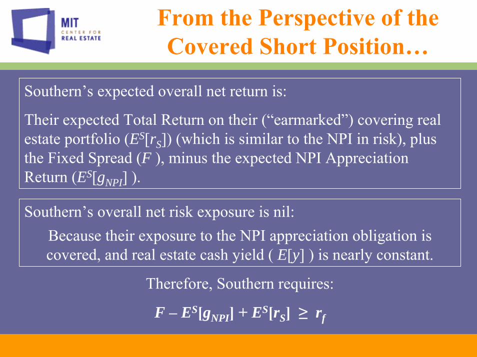
From the Perspective of the Covered Short Position…

Southern’s expected overall net return is:

Their expected Total Return on their (“earmarked”) covering real estate portfolio (ES[rS]) (which is similar to the NPI in risk), plus the Fixed Spread (F ), minus the expected NPI Appreciation Return (ES[gNPI] ).

Southern’s overall net risk exposure is nil:Because their exposure to the NPI appreciation obligation is covered, and real estate cash yield ( E[y] ) is nearly constant.

Therefore, Southern requires:

F – ES[gNPI] + ES[rS] ≥ rf

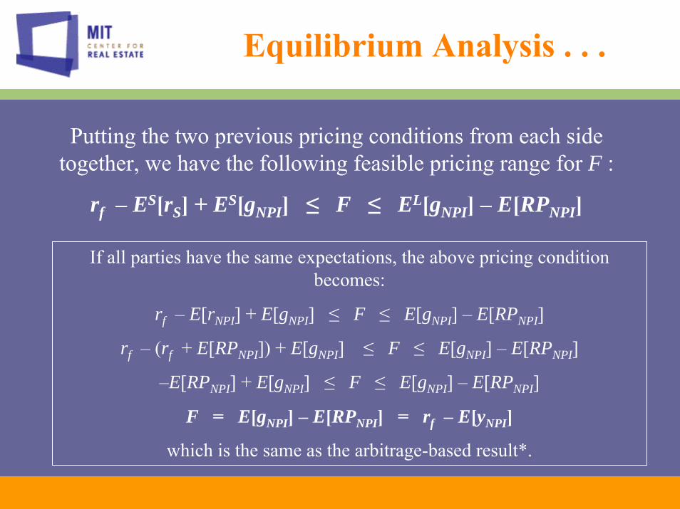
Putting the two previous pricing conditions from each side together, we have the following feasible pricing range for F :

rf – ES[rS] + ES[gNPI] ≤ F ≤ EL[gNPI] – E[RPNPI]


If all parties have the same expectations, the above pricing condition becomes:

rf – E[rNPI] + E[gNPI] ≤ F ≤ E[gNPI] – E[RPNPI]

rf – (rf + E[RPNPI]) + E[gNPI] ≤ F ≤ E[gNPI] – E[RPNPI]

–E[RPNPI] + E[gNPI] ≤ F ≤ E[gNPI] – E[RPNPI]

F = E[gNPI] – E[RPNPI] = rf – E[yNPI]

which is the same as the arbitrage-based result*.

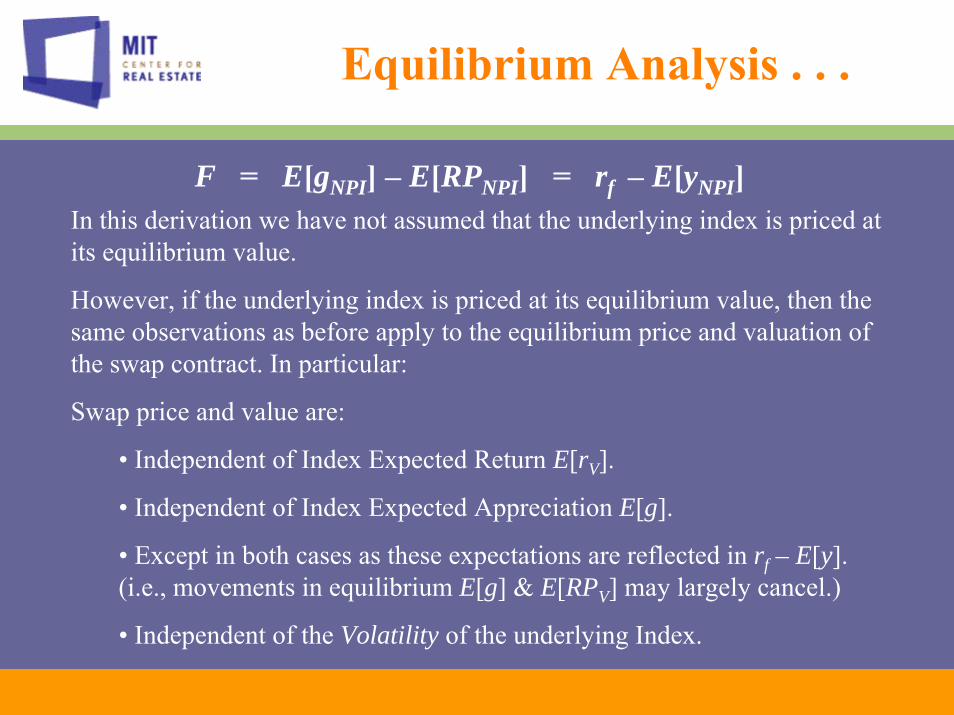
F = E[gNPI] – E[RPNPI] = rf – E[yNPI]In this derivation we have not assumed that the underlying index is priced at its equilibrium value.

However, if the underlying index is priced at its equilibrium value, then the same observations as before apply to the equilibrium price and valuation of the swap contract. In particular:

Swap price and value are:

• Independent of Index Expected Return E[rV].

• Independent of Index Expected Appreciation E[g].

• Except in both cases as these expectations are reflected in rf – E[y]. (i.e., movements in equilibrium E[g] & E[RPV] may largely cancel.)

• Independent of the Volatility of the underlying Index.


F = E[gNPI] – E[RPNPI] = rf – E[yNPI]There is an important corollary to this observation:

If real estate swap prices (spreads) are observed to move noticeably with:

• Changes in Index Expected Returns going forward E[rV] , OR

• Changes in Index Expected Appreciation going forward E[g],

• Beyond the movements implied by changes in rf – E[y] ,

Then:

The underlying index is not priced at equilibrium(e.g., the index value may be lagged behind current property market

equilibrium values due to the effect of appraisal valuation and/or other index construction issues.)


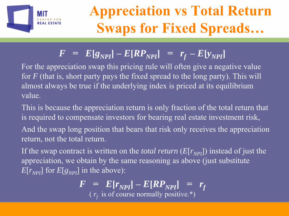
F = E[gNPI] – E[RPNPI] = rf – E[yNPI]For the appreciation swap this pricing rule will often give a negative value for F (that is, short party pays the fixed spread to the long party). This will almost always be true if the underlying index is priced at its equilibrium value.This is because the appreciation return is only fraction of the total return that is required to compensate investors for bearing real estate investment risk,And the swap long position that bears that risk only receives the appreciation return, not the total return.If the swap contract is written on the total return (E[rNPI]) instead of just the appreciation, we obtain by the same reasoning as above (just substitute E[rNPI] for E[gNPI] in the above):

F = E[rNPI] – E[RPNPI] = rf( rf is of course normally positive.*)

Appreciation vs Total Return Swaps for Fixed Spreads…

F = E[gNPI] – E[RPNPI] = rf – E[yNPI]The long-term historical average quarterly return components for the NPI are as follows (1978-2005):

E[gNPI] = 0.46%

E[RPNPI] = 0.90%

rf = 1.51%

E[yNPI] = 1.94%

Which implies a long-term average appreciation price, F of:

Typical Numbers…

F = 0.46% – 0.90% = 1.51% – 1.94% = – 0.43%


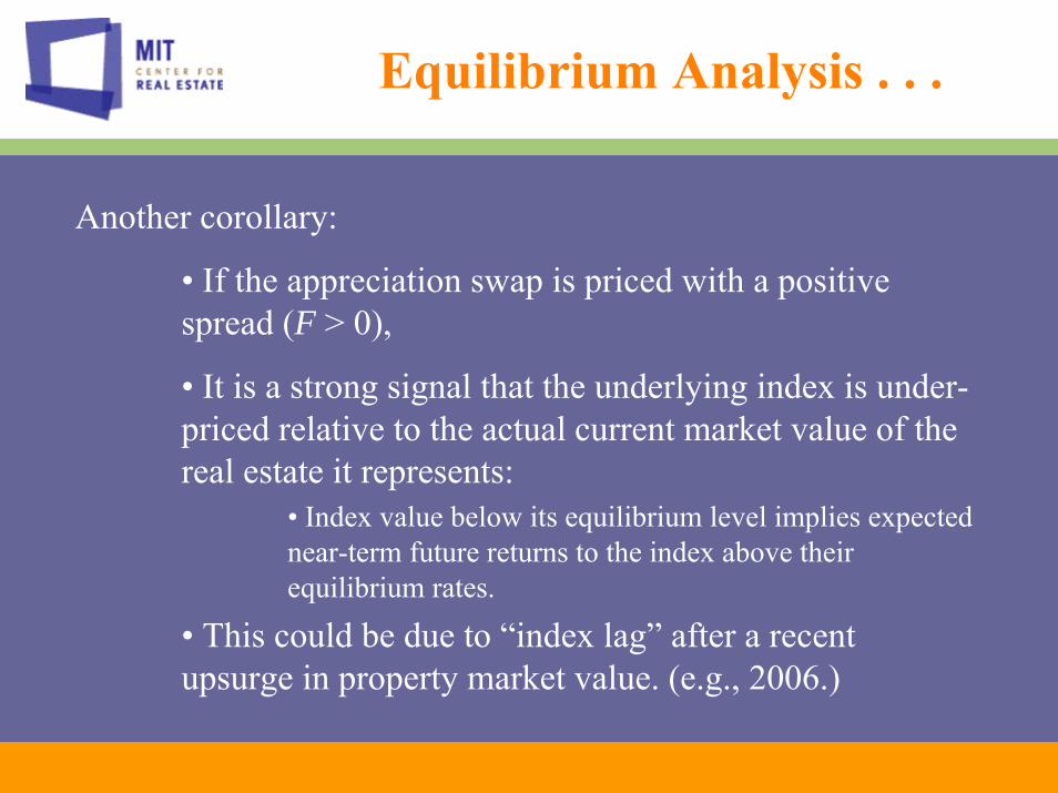
Another corollary:

• If the appreciation swap is priced with a positive spread (F > 0),

• It is a strong signal that the underlying index is under-priced relative to the actual current market value of the real estate it represents:

• Index value below its equilibrium level implies expected near-term future returns to the index above their equilibrium rates.

• This could be due to “index lag” after a recent upsurge in property market value. (e.g., 2006.)

Suppose over the period of the contract:

The potential long party expects gNPI will overperform 25 bps/qtr above the general market expectation:

EL[gNPI] = E[gNPI] + 25bps.

The potential short party is relatively bearish:ES[gNPI] = E[gNPI] – 25bps.

Suppose further that the potential short party feels that their own (covering) real estate portfolio will beat the NPI totalreturn by an average of 25bps/qtr (even though it contains the same risk as the NPI, i.e., the excess is “alpha” ):

ES[rS] = ES[rNPI] + 25bps

Effect of Heterogeneous Expectations…

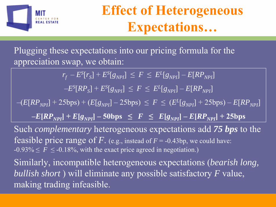
rf – ES[rS] + ES[gNPI] ≤ F ≤ EL[gNPI] – E[RPNPI]

–ES[RPS] + ES[gNPI] ≤ F ≤ EL[gNPI] – E[RPNPI]

–(E[RPNPI] + 25bps) + (E[gNPI] – 25bps) ≤ F ≤ (EL[gNPI] + 25bps) – E[RPNPI]

–E[RPNPI] + E[gNPI] – 50bps ≤ F ≤ E[gNPI] – E[RPNPI] + 25bps

Effect of Heterogeneous Expectations…

Plugging these expectations into our pricing formula for the appreciation swap, we obtain:

Such complementary heterogeneous expectations add 75 bps to the feasible price range of F. (e.g., instead of F = -0.43bp, we could have: -0.93% ≤ F ≤ -0.18%, with the exact price agreed in negotiation.)

Similarly, incompatible heterogeneous expectations (bearish long, bullish short ) will eliminate any possible satisfactory F value, making trading infeasible.

Type of Heterogeneity Useful for Trading…

Implication of the fact that the zero-NPV price condition can be expressed in either of two ways:

E[g] – E[RP] OR rf – E[y]

Apart from “alpha” considerations, in order to obtain complementary (overlapping) price requirements, we require:

Heterogeneity in gNPI expectations that are not canceled out by heterogeneity in RPNPI expectations. This requires:

Offsetting E[gNPI] & E[yNPI] expectations.e.g.: If the long party believes that NPI appreciation will be 1%/year higher than average it must also believe that NPI income yields will be 1%/year lower than average.

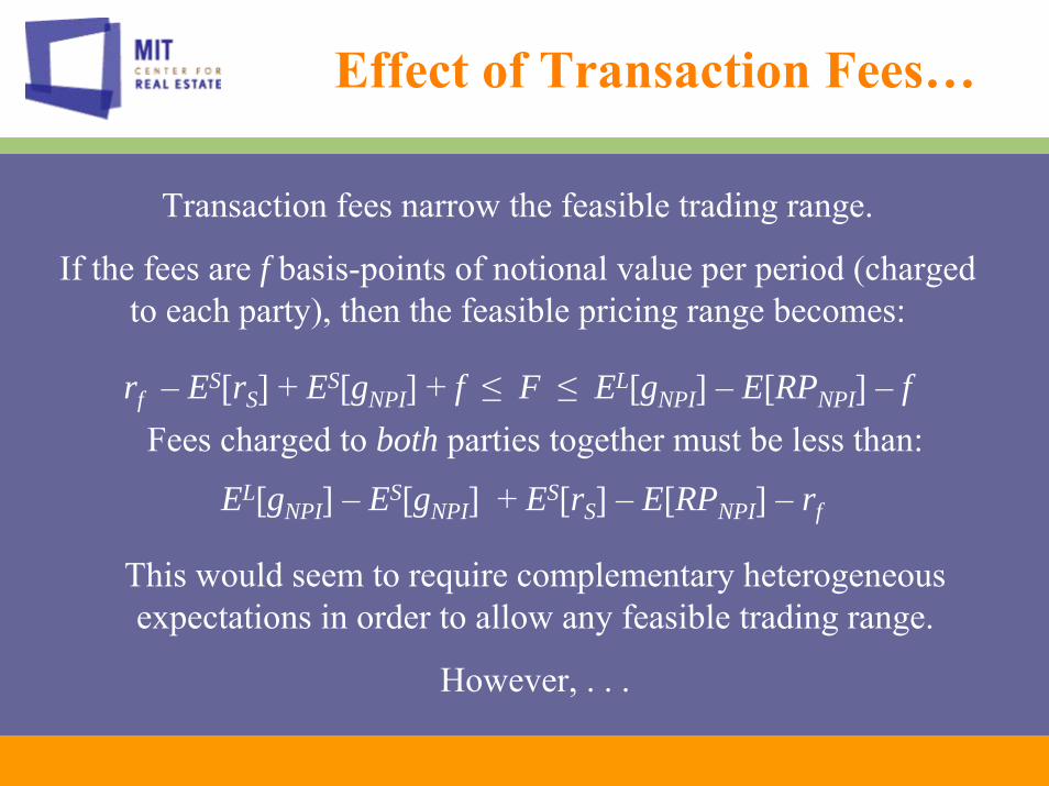
rf – ES[rS] + ES[gNPI] + f ≤ F ≤ EL[gNPI] – E[RPNPI] – f

Effect of Transaction Fees…

Transaction fees narrow the feasible trading range.

If the fees are f basis-points of notional value per period (charged to each party), then the feasible pricing range becomes:

This would seem to require complementary heterogeneous expectations in order to allow any feasible trading range.

However, . . .

EL[gNPI] – ES[gNPI] + ES[rS] – E[RPNPI] – rf

Fees charged to both parties together must be less than:

Effect of Transaction Fees…

The above analysis ignores the savings of transactions costs, investment management fees, and other advantages of using derivatives versus traditional methods of accomplishing the portfolio balancing or hedging/speculation objectives underlyingthe short and long positions.

For example, suppose the long party would avoid 20 bp/qtr in investment management and fund fees, and suppose the short partyeffectively saves 10 bp/qtr in costs of borrowing against their portfolio (alternative traditional methods to accomplish portfolio balancing objectives).

Then even with homogeneous expectations, there exists 30 bp/qtr of savings that can be split among the two parties and the brokers and investment banking fees of the derivative process.

What about predictability in the NPI?…

Appraisal smoothing and stale appraisals (along with true underlying property market sluggishness) give the NPI much more inertia than typical securities indexes, making the NPI relatively smooth and predictable.

Wouldn’t this type of predictability result in an absence of heterogeneous expectations, and thereby an absence of counterparties for trading the derivatives, making a functioningfutures market impossible?


Answer: Not necessarily.As seen in our Littleton & Southern example, derivative traders may have reasons other than speculation for trading derivatives. Heterogeneous expectations may not be necessary.

Predictability in the NPI will simply come out in the equilibrium derivative price, F.

Recall that F is a function of the market participants’ expectations about the future NPI appreciation returns: EL[gNPI] and ES[gNPI].

e.g., if NPI is headed down, then E[gNPI] will be negative, making F more negative than it would otherwise be (meaning the short position must pay the long position more in the fixed leg).

Well-functioning futures markets have long existed for various commodities and financial products whose future price directions are often rather predictable in advance (e.g., corn, wheat, oil, foreign exchange, among others).


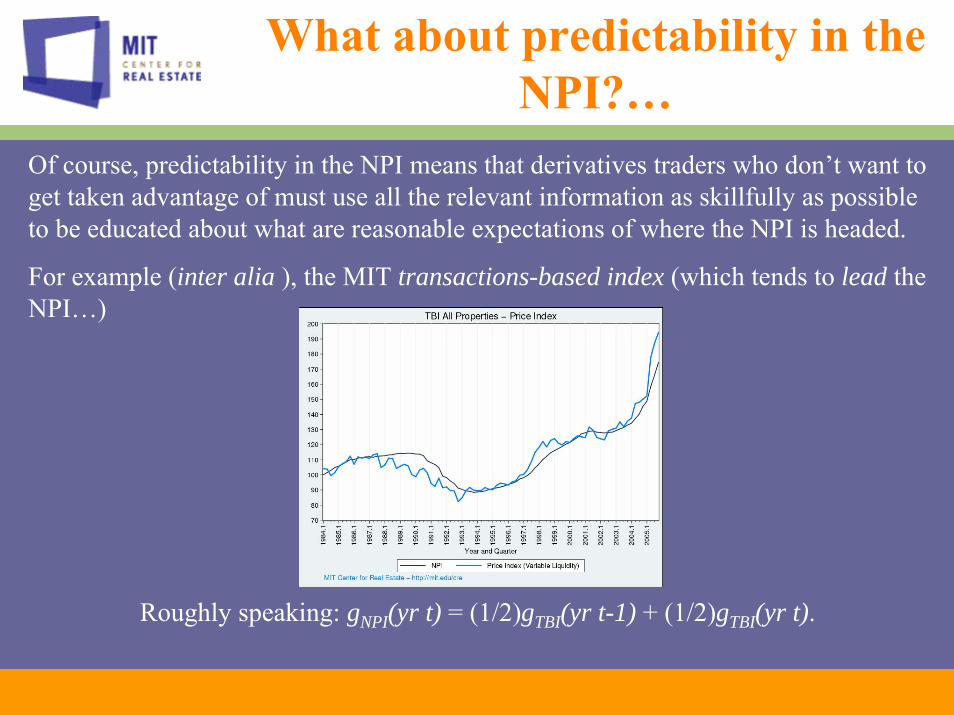
Of course, predictability in the NPI means that derivatives traders who don’t want to get taken advantage of must use all the relevant information as skillfully as possible to be educated about what are reasonable expectations of where the NPI is headed.

For example (inter alia ), the MIT transactions-based index (which tends to lead the NPI…)

Roughly speaking: gNPI(yr t) = (1/2)gTBI(yr t-1) + (1/2)gTBI(yr t).


Effect of Index Lag on Swap Pricing and Valuation:Effect of Index Lag on Swap Pricing and Valuation:Index Lag Index will often not be valued at its equilibrium value.That is, realistic expected returns on the index differ in the near-term from long-run equilibrium rates.In such circumstances, the Arbitrage Pricing and Valuation Formula for the swap no longer holds.The zero-NPV pricing condition will still be well approximated by:

F = E[g] – E[RPV]but not by rf – E[y], and only provided that E[RPV] in the above formula reflects the market’s long-run equilibrium risk premium, not the current disequilibrium premium presented by the index (while E[g] reflects the non-equilibrium appreciation in the index).

Alternative Pricing Perspectives…

The previous pricing analysis assumed trading by “covered”parties on both sides.Alternative pricing perspectives are possible…Suppose neither party is covered at all, and both view themselves as requiring a return as if they were actually making the notional investment. The resulting pricing condition would be:

rf + ES[gNPI] – E[RPNPI] ≤ F ≤ EL[gNPI] – rf – E[RPNPI]Which implies a feasible pricing range for F of width:

E[gLNPI] – E[gS

NPI] – 2rf

This requires that the long position be substantially more bullish than the short position. But this perspective is not based on an But this perspective is not based on an equilibrium framework . . .equilibrium framework . . .


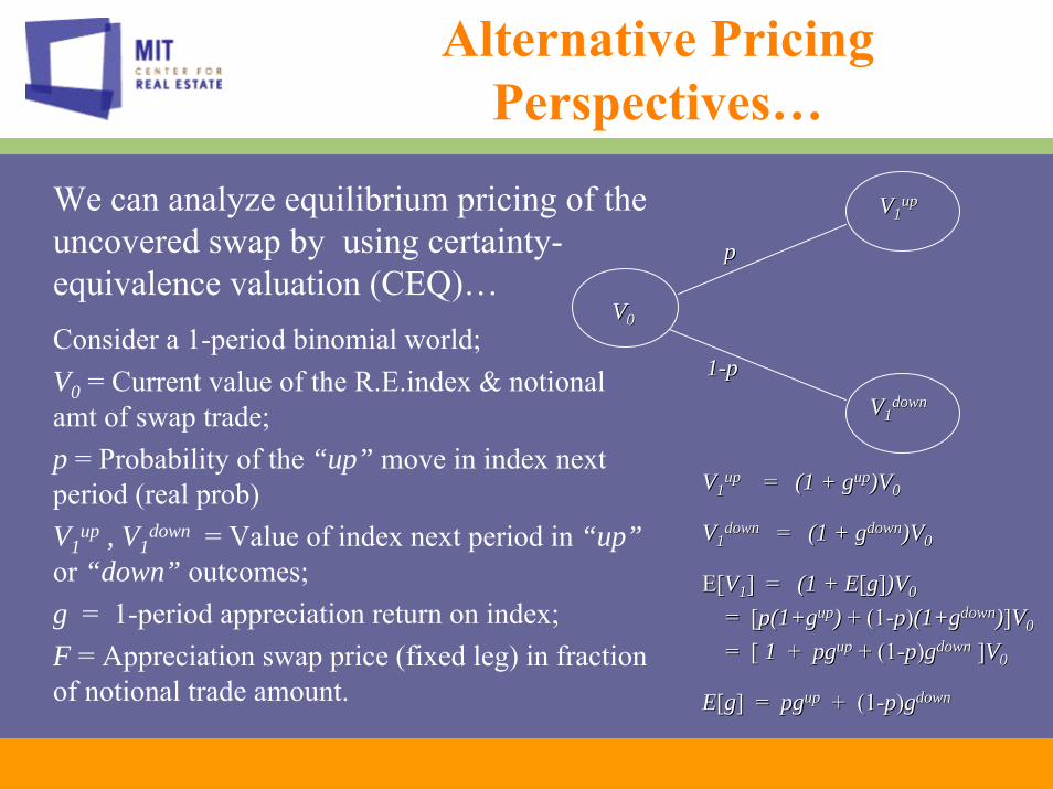
We can analyze equilibrium pricing of the uncovered swap by using certainty-equivalence valuation (CEQ)…Consider a 1-period binomial world;V0 = Current value of the R.E.index & notional amt of swap trade;p = Probability of the “up” move in index next period (real prob)V1

up , V1down = Value of index next period in “up”

or “down” outcomes;g = 1-period appreciation return on index;F = Appreciation swap price (fixed leg) in fraction of notional trade amount.

VV00

VV11upup

VV11downdown

pp

11--pp

VV11upup = = (1 + g(1 + gupup)V)V00

VV11downdown = = (1 + g(1 + gdowndown)V)V00

E[E[VV11] = ] = (1 + E(1 + E[[gg]])V)V00

= [= [p(1+gp(1+gupup)) + (1+ (1--pp))(1+g(1+gdowndown))]]VV00

= [ = [ 11 + + pgpgupup + (1+ (1--pp))ggdowndown ]]VV00

EE[[gg] = ] = pgpgupup + (1+ (1--pp))ggdowndown


Cash flow amts for apprec swap long position:Expected CF next period is:

00

CFCF11upup = = ((ggupup –– F)VF)V00

CFCF11downdown = = ((ggdowndown –– F)VF)V00

pp

11--pp

E[E[CFCF11] = [] = [pgpgupup + (1+ (1--pp))ggdowndown ]]VV00 –– FVFV00

= ( = ( EE[[gg] ] –– FF ))VV00

Certainty Equivalent CF next period is:CEQCEQ[[CFCF11] = ] = EE[[CFCF11] ] –– EE[[RPRPVV](](CFCF11

upup –– CFCF11downdown )/()/(VV11

upup//VV00 –– VV11downdown/V/V0 0 ))

= = EE[[CFCF11] ] –– ( ( EE[[rrVV] ] –– rrff )()(ggupup –– ggdowndown )V)V00 / (/ (ggupup –– ggdowndown ))

== EE[[CFCF11] ] –– ( ( EE[[rrVV] ] –– rrff ))VV00

Hence, present value of uncovered swap CF next period is:PVPV[[CFCF11] = [ ] = [ EE[[CFCF11] ] –– ( ( EE[[rrVV] ] –– rrff ))VV00 ] / (1 + ] / (1 + rrff ))

In equilibrium, this must equal the 0 net CF of the trade today:PVPV[[CFCF11] = [ ] = [ EE[[CFCF11] ] –– ( ( EE[[rrVV] ] –– rrff ))VV00 ] / (1 + ] / (1 + rrff ) = ) = 00 . . EE[[CFCF11] = ] = ( ( EE[[rrVV] ] –– rrff ))VV00


Thus, we have the equilibrium condition:

00

CFCF11upup = = ((ggupup –– F)VF)V00

CFCF11downdown = = ((ggdowndown –– F)VF)V00

pp

11--pp

EE[[CFCF11] = ] = ( ( EE[[rr] ] –– rrff ))VV00

( ( EE[[gg] ] –– FF ))VV00 = ( = ( EE[[rr] ] –– rrff ))VV00

FF = = rrff + + EE[[gg] ] –– EE[[rr] = ] = EE[[gg] ] –– EE[[RPRP]]

== rrff –– EE[[yy]]

This is the same equilibrium pricing condition that we obtained before:

F = E[g] – E[RP] = rf – E[y]

( )( ) ( )( )

( )Tf

Tf

TV

VT

Tf

TT r

rrErSTDCSTDCE

rCCEQCPV

+

+−+⎟⎟⎠

⎞⎜⎜⎝

⎛±

=+

=1

1][1][][][

1][][ 0

100

0

Certainty Equivalence Valuation of Derivatives…

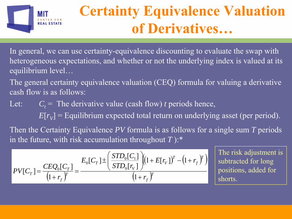
In general, we can use certainty-equivalence discounting to evaluate the swap with heterogeneous expectations, and whether or not the underlying index is valued at its equilibrium level…The general certainty equivalence valuation (CEQ) formula for valuing a derivative cash flow is as follows:Let: Ct = The derivative value (cash flow) t periods hence,

E[rV] = Equilibrium expected total return on underlying asset (per period).

Then the Certainty Equivalence PV formula is as follows for a single sum T periods in the future, with risk accumulation throughout T ):*

The risk adjustment is subtracted for long positions, added for shorts.


For the index swap, the CEQ valuation formula for a given future cash flow of the swap t periods in the future (Ct) with current value of the underlying index (= notional amount of trade) V0 is:

( )( )

( )

( )

( )

( )( ) .1

][][

1][

][][][

1][][][][

1][][

00

00

00

0

tf

Vt

tf

V

VVt

tf

V

tVt

tf

tt

rVRPECE

rrSTD

VrSTDRPECE

rrSTDCSTDRPECE

rCCEQCPV

+±

=

+

⎟⎟⎠

⎞⎜⎜⎝

⎛±

=

+

⎟⎟⎠

⎞⎜⎜⎝

⎛±

=+

=

There is only 1 period of risk accumulation (just prior to the cash flow), because the cash flow is based solely on the index return in period ttimes a notional amount that is fixed up front at time 0. Hence, the risk adjustment in the numerator is for just one period.

Where the risk adjustment in the numerator is subtracted for long positions and added for short positions (negative correl betwswap & index).

where E[RPV] is the mkt equilibrium risk premium.

Consider a 1-period example with F = -60bp and the following expectations:Long Perspective: rf = 0.75% /qtr Short Perspective:EL[rNPI] = 2.00% /qtr ES[rNPI] = 2.00% /qtrEL[gNPI] = 0.75% /qtr ES[gNPI] = 0.55% /qtrEL[RPNPI] = 1.25% /qtr ES[RPNPI] = 1.25% /qtrEL[C1] = (0.0075 – (-0.0060))$100 ES[C1] = (-0.0055 + (-0.0060))$100

= $0.75 + $0.60 = $1.35. = -$0.55 – $0.60 = -$1.15.Applying the certainty equivalence DCF valuation formula:


( ) ( ) 0993.0$0075.1

25.1$35.1$0075.1

100$0125.35.1$][][][ 110 =

−=

−=

−=

f

VtL

tL

RVRPECECPV

( ) ( ) 0993.0$0075.1

25.1$15.1$0075.1

100$0125.15.1$][][][ 110 =

+−=

+−=

−=

f

VtS

tS

RVRPECECPV

Because of heterogeneous expectations,The trade allows both sides to face a positive NPV ex ante.


PV[C] = CEQ[C] / (1+rf) = $0.10 / 1.0075 = $0.0993.Even though the expected cash flow is $1.35 for the long position, -$1.15 for the short position, the certainty equivalent cash flow is only $0.10 in both cases. The certainty-equivalence operation reverses the sign of the short position cash flow expectation, because the risk in the short position is negative the risk in the underlying index, because the two are perfectly negatively correlated.

( ) ( ) 0993.0$0075.1

25.1$35.1$0075.1

100$0125.35.1$][][][ 110 =

−=

−=

−=

f

VtL

tL

RVRPECECPV

( ) ( ) 0993.0$0075.1

25.1$15.1$0075.1

100$0125.15.1$][][][ 110 =

+−=

+−=

−=

f

VtS

tS

RVRPECECPV

Note that you should always employ the market equilibrium risk premium for the underlying index.

NPVL = +$0.0993.Same answer as before.

(But this formula only works if the underlying index is in equilibrium.)

Same thing using the arbitrage formula…

See downloadable Excel® file example on book CD

( )( )

( )0993.0$100$*13333.0*00744.0

100$0075.

0125.0060.10075.1

11

11

11)(

1

0

==

⎟⎠⎞

⎜⎝⎛ +−−⎟⎟

⎠

⎞⎜⎜⎝

⎛−=

⎟⎟⎠

⎞⎜⎜⎝

⎛ +−⎟

⎟⎠

⎞⎜⎜⎝

⎛

+−= NPI

rEyF

rlongNPV

fT

f

NPVS = +$0.0993.

Given the same conditions as before with F = -0.60%:rf = 0.75% /qtr

EL[rNPI] = 2.00% /qtr ES[rNPI] = 2.00% /qtrEL[gNPI] = 0.75% /qtr ES[gNPI] = 0.55% /qtr

Define:EyL = EL[rNPI] – EL[gNPI] = 2% – .75% = 1.25%EyS = ES[rNPI] – ES[gNPI] = 2% – .55% = 1.45%

Applying the arbitrage valuation formula to the $100 notional trade:

( )( )

( )0993.0$100$*13333.0*00744.0

100$10075.

0145.0060.0075.1

11

11

11)(

1

0

==

⎟⎠⎞

⎜⎝⎛ −

+−⎟⎟⎠

⎞⎜⎜⎝

⎛−=

⎟⎟⎠

⎞⎜⎜⎝

⎛−

+⎟⎟⎠

⎞⎜⎜⎝

⎛

+−= NPI

rEyF

rlongNPV

fT

f

Date post:	08-May-2018
Category:	Documents
Upload:	trankhue
View:	218 times
Download:	1 times

Real Estate Equity Derivatives - MIT OpenCourseWare Estate Equity Derivatives A derivative is an...

Documents