REAL OPTIONS AND THE MANAGEMENT OF R&D INVESTMENT: AN ANALYSIS OF COMPARATIVE ADVANTAGE, MARKET STRUCTURE, AND INDUSTRY DYNAMICS IN BIOTECHNOLOGY DISSERTATION Presented in Partial Fulfillment of the Requirements for the Degree Doctor of Philosophy in the Graduate School of The Ohio State University By Brian F. Lavoie, B.S., M.A. * * * * * The Ohio State University 2004 Dissertation Committee: Approved by Professor Ian M. Sheldon, Adviser Professor Eric O’N. Fisher ________________________________________________ Adviser Professor Mario J. Miranda Department of Agricultural, Environmental, and Development Economics
Transcript
REAL OPTIONS AND THE MANAGEMENT OF R&D INVESTMENT: AN ANALYSIS OF COMPARATIVE ADVANTAGE,
MARKET STRUCTURE, AND INDUSTRY DYNAMICS IN BIOTECHNOLOGY
DISSERTATION
Presented in Partial Fulfillment of the Requirements for
the Degree Doctor of Philosophy
in the Graduate School of The Ohio State University
By
Brian F. Lavoie, B.S., M.A.
* * * * *
The Ohio State University 2004
Dissertation Committee: Approved by Professor Ian M. Sheldon, Adviser Professor Eric O’N. Fisher ________________________________________________
Adviser Professor Mario J. Miranda Department of Agricultural, Environmental, and Development Economics
ABSTRACT
This study examines the US comparative advantage in biotechnology vis-à-vis other Northern
countries, and the pattern of biotechnology industry dynamics emerging from the early entry of start-ups
and the lagged entry of multinationals. The development of high technology industries like biotechnology
is heavily influenced by the R&D investment behavior of firms active in the industry. Many theoretical
treatments of R&D investment tend to be excessively stylized, emphasizing the outcome, rather than the
process, of investment. In doing so, they neglect key characteristics of biotechnology R&D investment.
In contrast, real options theory represents investment as a dynamic process, extending over
multiple time periods, and continuously impacted by evolving conditions in the stochastic investment
environment. Real options incorporate the principle that firms actively manage their investments, adapting
investment strategies in response to the gradual resolution of ongoing uncertainty surrounding the
investment. This corresponds to the general structure of biotechnology R&D investment.
A real options model of investment with uncertain cost was used to analyze the source of the US
comparative advantage in biotechnology vis-à-vis Europe, its closest rival. Empirical evidence suggests two
sources of heterogeneity in the biotechnology R&D process: US biotechnology firms, on average, invest in
R&D at a faster per-period rate, and face a less uncertain domestic regulatory regime, than European
biotechnology firms. This leads to a cross-country asymmetry in strategies for managing the option to
invest in biotechnology R&D: more specifically, US firms impose a less rigorous decision criterion, vis-à-
vis European firms, to evaluate and manage their biotechnology R&D investment opportunities.
ii
Computer simulation was used to examine the implications of this result for the average R&D
investment behavior of representative US and European biotechnology firms. The simulation results
suggest that, on average, US biotechnology firms initiate more R&D projects, commence investment
sooner, innovate more rapidly, persevere longer in the face of mounting R&D costs, are less selective about
potential projects based on expected return, and ultimately, successfully complete more projects, than their
European counterparts. This supplies a plausible explanation for the emergence of the US as the world
leader in biotechnology, relative to other Northern countries, based on the key insight that the US
comparative advantage lies within the structure of the economic process central to leadership in high
technology industries: the ability to create, develop, and commercialize new technologies.
Real options were also used to analyze the pattern of biotechnology industry dynamics emerging
from the R&D investment behaviors of start-ups and multinationals. In general, start-ups have a greater
ability to attract elite scientific talent, but multinationals have access to deeper, more stable pools of
investment capital. Heterogeneity in the R&D investment process takes the form of a higher degree of
technical uncertainty and a higher maximum per-period rate of investment for multinationals relative to
start-ups. It also creates the possibility for type-specific investment strategies. Start-ups, by selling their
proprietary knowledge stocks, can reduce the irreversibility of R&D investment. Multinationals, by
purchasing contract research from start-ups, can partially resolve technical uncertainty without fully
committing to investment; if conditions warrant, the multinational can enter the R&D process midstream by
acquiring a start-up’s proprietary knowledge stock. These type-specific strategies can account for a pattern
of industry dynamics where start-ups, on average, enter the industry prior to multinationals.
A discrete-time real option investment model was developed to represent the R&D decisions of
start-ups and multinationals. Analysis of the model’s properties and comparative statics indicates that over
a range of parameter values, the multinational maximizes the value of its R&D investment opportunity by
delaying full commitment in favor of a limited investment in contract research to resolve technical
uncertainty. The start-up’s optimal strategy is to exercise its option to invest immediately. Availability of
the type-specific investment strategies tends to enhance the value of R&D investment opportunities, and
increase the range of economically feasible R&D investments, for both types of firms, relative to the case
where these strategies are not available. Computer simulation of the R&D investment behavior of
multinationals and start-ups produces a pattern of industry dynamics characterized by start-ups’ early entry
and multinationals’ late entry. The simulation also demonstrates that the type-specific strategies favorably
impact the value of the option to invest according to a number of measures, including average total R&D
expenditures, average net returns, average time to build, and the extent of down-side risk.
iii
This dissertation is dedicated to my wife Carol, to my parents Francis and Jane Lavoie,
and to my parents-in-law James and Linda Ziccardi.
iv
ACKNOWLEDGMENTS I wish to thank my adviser, Dr. Ian M. Sheldon, for his commitment to my doctoral work, and for
demonstrating how to conduct economics research with intellectual rigor and clarity of expression. I would
also like to acknowledge my debt to him for sharpening many of the ideas and insights found in this
dissertation, through the patient reading and discussion of many drafts. His willingness to take the time to
point out my more egregious lapses in writing style is also appreciated.
I would also like to thank my Dissertation Committee members, Dr. Eric O’N. Fisher and Dr.
Mario J. Miranda. Even after lengthy periods of inactivity on my part, requests for their participation in the
next stage of the work were always accepted promptly and enthusiastically. Dr. Fisher recommended the
Dixit and Pindyck book Investment Under Uncertainty to me, which ended up as the starting point for my
research. Dr. Miranda provided me with a copy of MatLab, and early drafts of his numerical methods
textbook (co-authored with Dr. Paul Fackler) served as my introduction and guide to computational
economics.
Comments from Dr. James Oehmke, of Michigan State University, motivated my analysis of the
R&D investment behaviors of start-ups and multinationals. Dr. Paul Fackler, of North Carolina State
University, provided MatLab algorithms to solve the dynamic programming problem in Chapter 4.
Finally, I would like to thank Dr. Edward O’Neill, Consulting Research Scientist, OCLC
Research, and Lorcan Dempsey, Vice President, OCLC Research, for easing my work responsibilities and
granting me time to complete my dissertation. I would especially like to thank Dr. O’Neill for never failing
to remind me over the course of a long series of annual reviews that I still had not finished my dissertation,
and for his persistence in including it as one of my goals for the coming year.
v
VITA
1988 ............................................................................ B.S. Economics, Ohio University 1990 ............................................................................ M.A. Economics, Ohio University 1990 ............................................................................ Certificate in Contemporary History, Contemporary History Institute, Ohio University
1990 – 1992 ................................................................ Graduate Teaching and Research Associate, The Ohio State University
1995 – 1996 ................................................................ Graduate Teaching Associate, The Ohio State University 1996 – 1998 ................................................................ Research Assistant, OCLC Inc. 1998 – 1999 ................................................................ Systems Analyst, OCLC Inc. 1999 – 2001 ................................................................ Associate Research Scientist, OCLC Inc. 2001 – present ............................................................ Research Scientist, OCLC Inc.
PUBLICATIONS Lavoie, B.F., and I.M. Sheldon. 2000. The source of comparative advantage in the biotechnology industry:
A real options approach. Agribusiness 16:56-67. Lavoie, B.F., and I.M. Sheldon. 2000. The comparative advantage of real options: An explanation for the
US specialization in biotechnology. AgBioForum 3, no. 1. http://www.agbioforum.org/v3n1/v3n1a07-lavoie.htm
Lavoie, B.F., and I.M. Sheldon. 2001. Market structure in biotechnology: Implications for long-run
comparative advantage. In Market development for genetically modified foods, ed. V. Santaniello, R.E. Evenson, and D. Zilberman, 291-300. Wallingford: CABI Publishing.
FIELDS OF STUDY Major Field: Agricultural, Environmental, and Development Economics Minor Field: International Economics
vi
TABLE OF CONTENTS
Page
Abstract ......................................................................................................................................................... ii
Dedication .................................................................................................................................................... iv
Acknowledgments ......................................................................................................................................... v
Vita ............................................................................................................................................................... vi
List of Tables ................................................................................................................................................. x
List of Figures ............................................................................................................................................. xii
Introduction ................................................................................................................................................... 1 Chapters: 1. Biotechnology: Science and Industry ........................................................................................................ 8
1.1 Biotechnology and Its Applications ................................................................................................. 8 1.1.1 Definition of Biotechnology .................................................................................................. 8 1.1.2 Commercial Applications ....................................................................................................... 9
1.2 The Biotechnology Industry ........................................................................................................... 12 1.2.1 Overview of the Global Industry .......................................................................................... 12 1.2.2 Evidence of US Specialization ............................................................................................. 15 1.2.3 Biotechnology R&D Investment .......................................................................................... 18
1.3 Structure and Dynamics of the Biotechnology Industry ................................................................. 20 1.3.1 Start-ups ............................................................................................................................... 21 1.3.2 Multinationals ...................................................................................................................... 23 1.3.3 Industry Dynamics ............................................................................................................... 24
1.4 Stylized Description of Biotechnology R&D Investment .............................................................. 26 1.5 Two Economic Questions .............................................................................................................. 27
2. Comparative Advantage and Dynamics in High Technology Industries ................................................. 28
2.2.1 The Factor Proportions Theory ............................................................................................ 29 2.2.2 Beyond Factor Proportions .................................................................................................. 32
2.2.2.1 Increasing Returns to Scale and Product Differentiation ........................................... 33 2.2.2.2 Strategic Trade Policy ................................................................................................ 34 2.2.2.3 The Role of History ................................................................................................... 35 2.2.2.4 Technology and Trade ............................................................................................... 36
2.3 Dynamic Open Economies with Endogenous Innovation .............................................................. 36 2.3.1 Innovation as an Endogenous Process ................................................................................. 36
vii2.3.2 Endogenous Innovation with International Technology Spillovers ..................................... 39
2.3.3 Endogenous Innovation with Limited Technology Spillovers ............................................. 44 2.4 The Grossman and Helpman Approach: Evaluation ...................................................................... 48
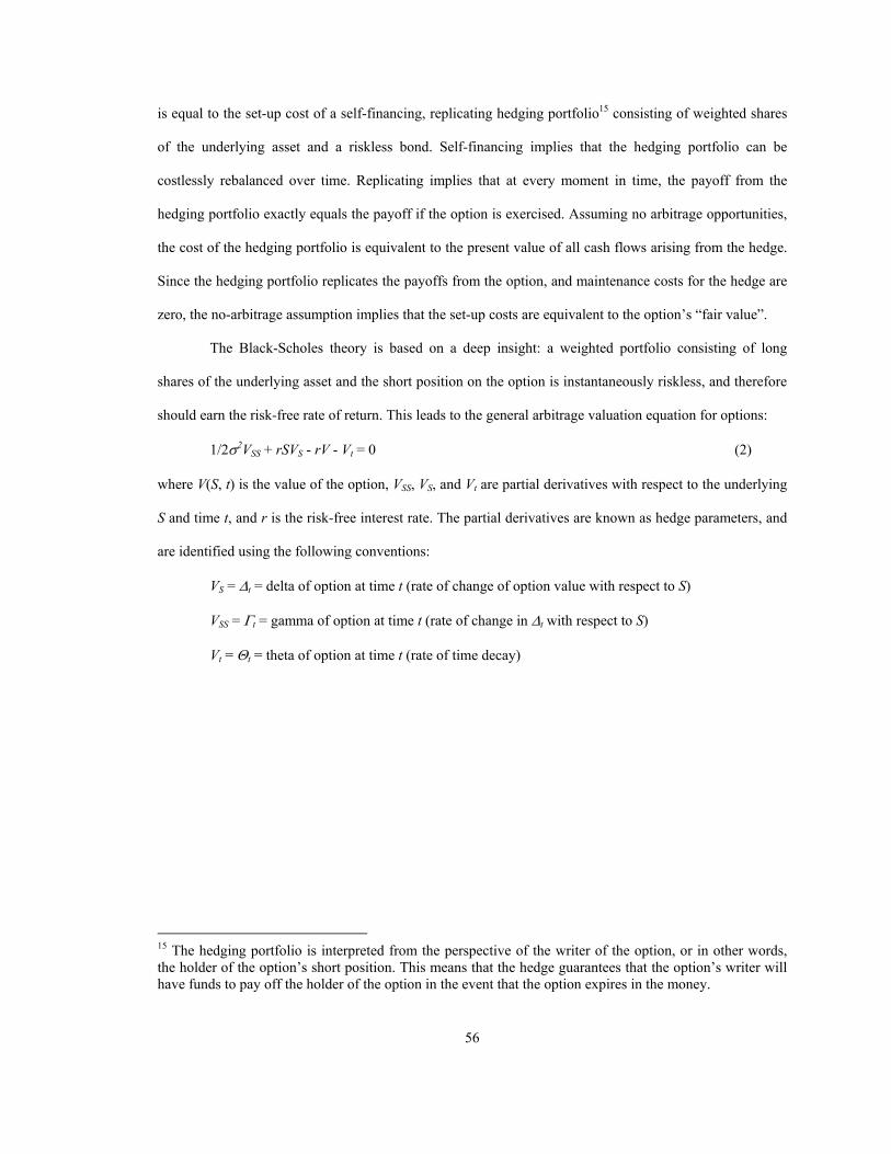
3. Real Options and Biotechnology R&D Investment ................................................................................. 51
3.1 Investment and the Supply of Capital ............................................................................................ 51 3.2 The Neoclassical Theory of Investment ......................................................................................... 53 3.3 Options and Option Pricing ............................................................................................................ 54 3.4 The Real Options Theory of Investment ........................................................................................ 58
3.4.1 Optimal Investment Strategies with Uncertain Value .......................................................... 60 3.4.2 Optimal Investment Strategies with Uncertain Cost ............................................................ 61
3.5 Real Options and Biotechnology R&D Investment ....................................................................... 64
4. Comparative Advantage in the Biotechnology Industry .......................................................................... 66
4.1 The First Economic Question Re-stated ......................................................................................... 67 4.2 Empirical Context .......................................................................................................................... 68
4.2.1 Candidate Sources of Heterogeneity in Biotechnology R&D .............................................. 69 4.2.1.1 Level of Irreversibility ............................................................................................... 69 4.2.1.2 Time to Build and the Per-period Rate of Investment ................................................ 71 4.2.1.3 Uncertainty ................................................................................................................. 73
4.2.2 Sources of Heterogeneity: Empirical Evidence .................................................................... 76 4.2.2.1 The Per-period Rate of Investment ............................................................................ 76 4.2.2.2 The Level of Exogenous Cost Uncertainty ................................................................ 78 4.2.2.3 Towards an Explanation for the US Comparative Advantage in Biotechnology ....... 81
4.3 A Real Options Model of Biotechnology R&D Investment ........................................................... 81 4.4 Comparative Statics........................................................................................................................ 86
4.4.1 A Solution Method for K* .................................................................................................... 87 4.4.2 Comparative Statics of K* and the Incentive to Invest ........................................................ 90 4.4.3 Implications for the First Economic Question ..................................................................... 99
4.5 Dynamic Stochastic Simulation ................................................................................................... 101 4.5.1 Computer Simulation of Biotechnology R&D Investment Behavior ................................. 102 4.5.2 Implementing the Simulation ............................................................................................. 104 4.5.3 Running the Simulation ...................................................................................................... 106 4.5.4 Results and Analysis .......................................................................................................... 109
4.6 Summary and Conclusion ............................................................................................................ 114
5. Market Structure and Industry Dynamics .............................................................................................. 117 5.1 The Second Economic Question Re-stated .................................................................................. 118 5.2 Classes of Firms in the Biotechnology Industry ........................................................................... 119
5.2.1 Sources of Heterogeneity Across Firm Types .................................................................... 119 5.2.2 Implications for Investment Behavior ................................................................................ 121
5.4 A New Model for Biotechnology R&D Investment ..................................................................... 128 5.4.1 General Structure ............................................................................................................... 128 5.4.2 Technical Uncertainty ........................................................................................................ 129
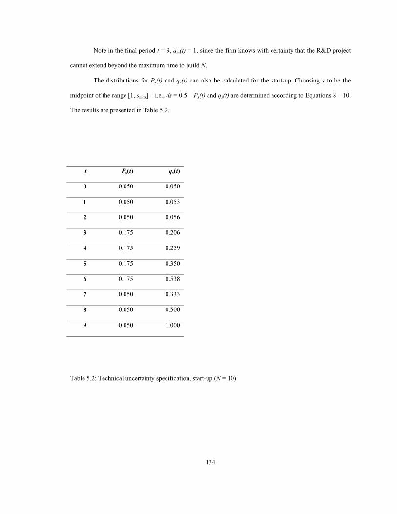
viii5.4.2.3 Example ................................................................................................................... 133
5.4.3 The Multinational’s R&D Investment Problem ................................................................. 135 5.4.4 The Start-up’s R&D Investment Problem .......................................................................... 140
5.5 Implementation and Example ....................................................................................................... 144 5.5.1 Parameter Vector ................................................................................................................ 144 5.5.2 Implementation Issues ........................................................................................................ 146 5.5.3 Description of the Computer Model ................................................................................... 146 5.5.4 Example ............................................................................................................................. 149
5.7 Simulation .................................................................................................................................... 175 5.7.1 Average Behavior .............................................................................................................. 176
5.8 Summary and Conclusion ............................................................................................................ 181
6. Conclusion ............................................................................................................................................. 184 6.1 Summary ...................................................................................................................................... 184 6.2 Implications and Directions for Future Research ......................................................................... 187
6.2.1 Entrepreneurialism ............................................................................................................. 187 6.2.2 Innovative Fringe ............................................................................................................... 190 6.2.3 Moral Hazard of Reversible Investment ............................................................................ 193
List of References ...................................................................................................................................... 197
ix
LIST OF TABLES Table Page 1.1 US imports, exports, and trade balance in biotechnology products, 1990-1999 (millions of dollars) .. 14
1.2 US and European biotechnology industries, 2000 ............................................................................... 16
1.3 International patent families in genetic engineering(selected countries): 1990-1994 .......................... 17
1.4 US venture capital disbursements: 1980-2000 (millions of dollars) .................................................... 23
3.1 Critical cost of kilowatt of capacity and value of option for mean expected cost (dollars) .................. 63
4.1 Average point elasticity of K* with respect to exogenous parameters ................................................. 94
4.2 Simulation outcome space .................................................................................................................. 103
5.3 Sample calibration of R&D investment models ................................................................................. 150
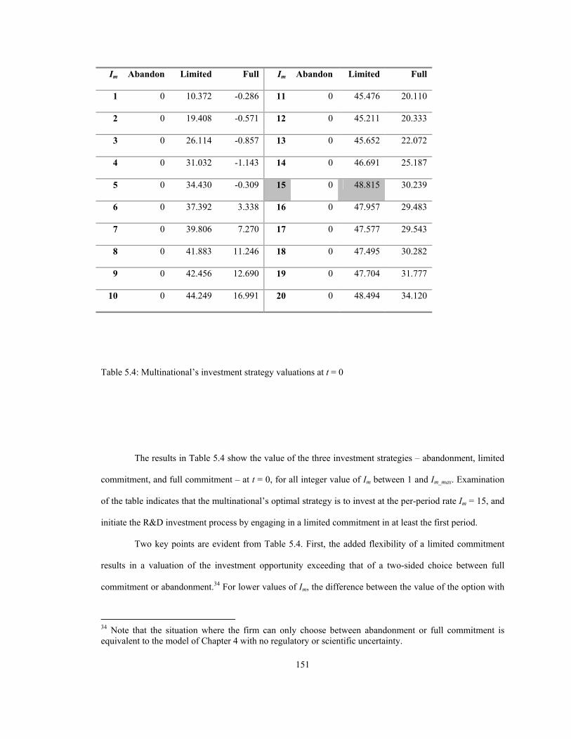
5.4 Multinational’s investment strategy valuations at t = 0 ...................................................................... 151
5.5 Start-up’s investment strategy valuations at t = 0 .............................................................................. 153
5.6 Optimal investment strategies and investment values, as functions of c ............................................ 157
5.7 Optimal investment strategies and investment values, as functions of µ .......................................... 158
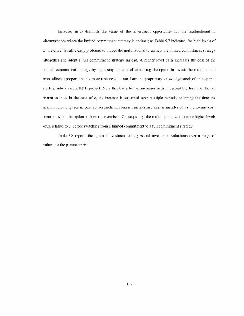
5.8 Optimal investment strategies and investment values, as functions of ds .......................................... 160
5.9 Optimal investment strategies and investment values, as functions of ρ ........................................... 163
5.10 Investment values, as function of Im_max and Is_max ............................................................................ 165
5.11 High, low, and intermediate values for exogenous parameters ........................................................ 168
5.12 Summary results for multinational and start-up ............................................................................... 169
x
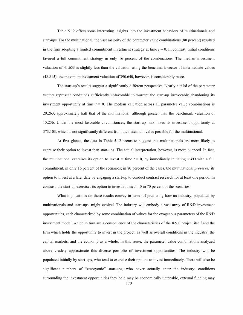
5.13 Start-up’s median valuation for parameter combinations containing low, intermediate, or high values of exogenous parameters ........................................................................................... 171
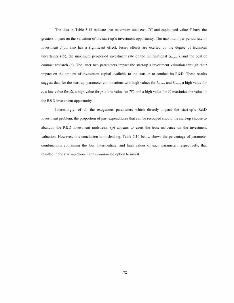
5.14 Fraction of parameter combinations containing low, intermediate, or high values of exogenous parameters resulting in abandonment strategy ............................................................... 173
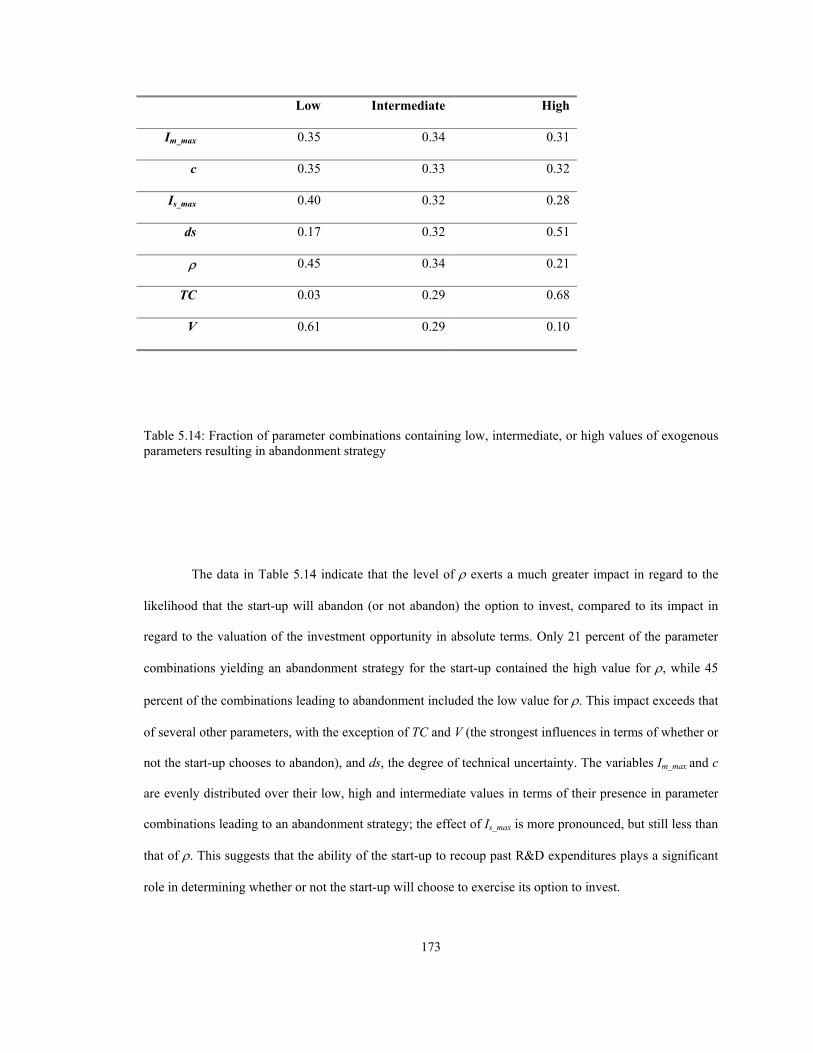
5.15 Multinational’s median valuation for parameter combinations containing low, intermediate, or high values of exogenous parameters ..................................................................... 174
5.16 Average R&D investment behavior, multinational and start-up ...................................................... 177
xi
LIST OF FIGURES Figure Page 2.1 Trade equilibrium ................................................................................................................................. 43
4.1 Value of investment opportunity, F(K), based on US and European benchmark vectors .................... 97
4.2 Sample time paths .............................................................................................................................. 107
5.1 Decision tree for multinational’s R&D investment problem (N = 5) ................................................. 139
5.2 Decision tree for start-up’s R&D investment problem (N = 5) .......................................................... 143
5.3 Per-period rate of investment as function of maximum rate, multinational and start-up ................... 166
xii
INTRODUCTION
Commercial biotechnology has been and continues to be the nearly exclusive province of
American firms. From the industry’s nascent stages to the present, biotechnology research and production
has concentrated in the United States, rather than in other Northern countries like Japan or those of Western
Europe. By the mid-1990s, US biotechnology firms “account[ed] for more than two-thirds of global sales –
virtually all major product introductions – and the majority of research and development spending”.
(Sawinski and Mason 1996, 73) In 2000, the US biotechnology industry earned three times the revenue,
spent three times as much on R&D, and employed nearly three times as many workers as the entire
European industry. (Ernst & Young 2001a, 5; Ernst & Young 2001b, 4) Casual inspection of the evidence
is enough to confirm US leadership in the biotechnology industry. This suggests an obvious question: why
did the United States emerge as the world leader in biotechnology, vis-à-vis other Northern countries?
Biotechnology is populated by two distinct classes of firms: start-ups – small, nimble companies
set up to commercialize leading-edge research; and multinationals – large, mature corporations managing
an extended portfolio of established product lines. The present state of commercial biotechnology is the
result of a dynamic process of industry development propelled by the asymmetric, yet complementary
investment behaviors of each class of firm. Start-ups were early entrants to the industry, investing vast
sums in R&D in hopes of realizing commensurately large returns from the successful introduction of new
products. Multinationals eschewed early commitment to biotechnology in favor of a “wait and see”
strategy. As the industry stabilized and commercial opportunities came more sharply into focus,
multinationals entered the industry in greater numbers, often through R&D partnerships or licensing
arrangements with, or the outright acquisition of, existing start-ups. This description of biotechnology’s
market structure and industry dynamics prompts another question: why did start-ups, on average, choose to
exploit their opportunities in biotechnology prior to multinationals?
1
The two questions posed above represent alternative ways of stating a single problem that surfaces
regularly in economics: the efficient decentralization of economic activities. Decentralization can occur
across time (intertemporal resource allocation), space (cross-country patterns of specialization), and even
productive agents (workers or firms). Regardless of the context, the problem retains elements common to
all instances: two or more economic agents, differentiated on the basis of one or more characteristics – e.g.,
time of existence, country of origin, corporate structure, skill set, etc. The problem also specifies one or
more economic activities, the outcome of which (measured in a variety of ways, such as quantity produced)
is impacted by the defining characteristics of the economic agents. Given these conditions, the salient
economic question is to predict, or from a normative perspective, stipulate, the distribution of economic
activities across the various classes of economic agents.
International trade theory resolves the decentralization problem through the classic principle of
comparative advantage, which organizes economic activities across countries based on international
differences in “primitive elements” such as technology or resource endowments. The first question posed
above is a straightforward expression of the comparative advantage problem.
Although it may not be readily apparent, the second question is another version of the same
problem. Here, economic agents are distinguished not by country of origin, but by corporate structure: i.e.,
start-up or multinational. Differences across classes of firm – for example, in the relative ease of access to
investment capital – impact economic decision-making in regard to R&D and production. The logical
progression of the problem in this context mirrors that in the case where differences are associated with
geographical origin: the distinguishing characteristics of the economic agents lead to differing economic
behaviors, which ultimately shape the distribution of economic activities across classes of agents.
Since both questions posed above are based on a well-defined problem in economic theory, it is
reasonable to expect they can be easily answered by appealing to the existing literature. But on closer
inspection, this literature proves less than satisfactory when applied to the biotechnology industry. Models
treating the pattern of specialization in high technology industries1 like biotechnology usually attribute
1 Tyson (1993) defines a high technology industry as “one in which knowledge is a prime source of competitive advantage for producers, who in turn make large investments in knowledge creation.
2
comparative advantage to traditional sources of heterogeneity such as inherited resource endowments. This
approach is appropriate for determining why a country like the United States specializes in biotechnology:
disparities in the relative composition of resource endowments between countries in the developed North
and those in the developing South create cost differentials favoring Northern countries, which, in general,
are relatively abundant in resources such as skilled labor or human capital. This implies that the bulk of
research and production in biotechnology will concentrate in a Northern country like the United States.
But inherited resource endowments are much less useful for explaining why the US in particular
specializes in biotechnology. Here, the comparison is between two Northern countries, and in this context,
the usual chain of reasoning breaks down in the face of empirical evidence. As Helpman and Krugman
(1985, 2) point out, “Conventional trade theory explains trade entirely by differences among countries,
especially differences in their relative endowments of factors of production … In practice, however, nearly
half the world’s trade consists of trade between industrial countries that are relatively similar in their
relative factor endowments.” Absent the presence of heterogeneity, the identity of the world leader in a
given industry becomes arbitrary in a trading community populated by similar countries. In this sense,
existing theories of international trade which derive comparative advantage from cross-country
heterogeneity in inherited resource endowments fall short in explaining the US leadership in biotechnology.
Avoiding an arbitrary solution to the pattern of specialization in biotechnology requires the
identification of some form of heterogeneity to differentiate economic incentives across countries. A likely
source of this heterogeneity is the process of R&D investment. Like many high-technology industries,
biotechnology is an R&D-intensive activity, where the realization of potentially large, yet highly uncertain
returns are preceded by substantial commitments of investment capital over an often lengthy time horizon.
Entering the biotechnology industry is, in effect, equivalent to making the decision to undertake a program
of biotechnology R&D investment. It is likely, then, that comparative advantage in biotechnology emerges
from cross-country differences in the incentives to invest in biotechnology R&D.
Reflecting this definition, high technology industries are usually identified as those with above-average spending on research and development, above-average employment of scientists and engineers, or both.”
3
Existing models of specialization and trade in high technology industries tend to represent the
R&D investment process in a heavily stylized way, often as little more than an economic “bet”: a firm has
the opportunity to invest some specified amount of capital in hopes of receiving an uncertain return
governed by a known probability distribution. The investment decision rule is based on the net present
value of the investment: the difference between the expected discounted stream of benefits and the
expected discounted stream of costs. If the result is positive, the firm invests. Typically, the outcome is
revealed instantaneously: either the R&D yields a new product next period, or it never will.
This characterization of R&D investment is adequate for many purposes, but in regard to
biotechnology, it falls short on several counts. Biotechnology R&D investment has a distinct structure,
comprised of a number of key features. This structure and its accompanying features extend well beyond
what a terse representation of R&D investment can express. The structure of biotechnology R&D
investment has important implications for the decision rule used to evaluate investment opportunities, not
only in terms of the initial decision whether to invest, but also in regard to managing the R&D investment
process over its duration.
The need for a richer exposition of the biotechnology R&D investment process extends to the
second question posed above, concerning biotechnology’s industry dynamics. The distribution of
biotechnology activities across classes of firms can be viewed as a problem in dynamic comparative
advantage. In the early stages of the biotechnology industry, start-ups perceived greater incentives, relative
to multinationals, to enter the industry by investing in biotechnology R&D; consequently, biotechnology
R&D and production were initially concentrated within this class of firm. As the industry matured,
multinationals entered the industry at a more rapid pace, presumably in response to enhanced investment
incentives. As a result, the start-ups’ comparative advantage in biotechnology began to erode, as the
industry reflected the growing presence of multinationals, in concert with a steady process of consolidation.
It is likely that the sources of heterogeneity which at first favored start-ups, and then multinationals – i.e.,
which shifted comparative advantage across classes of firms – are also derived from the structure of R&D
investment. A thorough description of biotechnology R&D is needed to identify sources of heterogeneity
relevant for explaining the distribution of biotechnology activities across start-ups and multinationals.
4
Given the fundamental similarity between determining the source of comparative advantage in
biotechnology across countries and across classes of firms, it would be useful to employ a single, unifying
framework to examine these problems. The real options theory of investment offers such a framework. Real
option investment models are based on three observed characteristics of investment: irreversibility, ongoing
uncertainty, and flexible timing. Taking these characteristics into account, the opportunity to invest can be
likened to holding a financial option, except that the option is “written” on a real asset, rather than a
financial instrument. The firm holds the right, but not the obligation, to initiate investment. When a firm
invests, it irrevocably “kills” the option to delay investment and observe evolving conditions in the
stochastic investment environment. The value of this lost flexibility must be included in the cost of
investment. As a result, the return necessary to induce a firm to invest tends to exceed the cost of capital.
Pricing models used to value financial options can be used to derive optimal investment strategies
in the presence of the option to invest. It can be shown that investment strategies – i.e., decision rules for
managing and exercising the option to invest – are heavily influenced by factors such as the necessity to
invest incrementally, the presence of time to build, the degree and type of uncertainty, and the rate of
productive investment. Significantly, these factors coincide with the principal features of R&D investment
in the biotechnology industry. This suggests that real options investment models are well suited for
analyzing R&D investment behavior in the biotechnology industry, and in particular, the sources of
heterogeneity leading to asymmetric investment behaviors across countries and types of firms.
The presence of heterogeneity in the structure of biotechnology R&D leads to a corresponding
asymmetry in optimal investment rules. Differences in these rules across countries or classes of firms imply
heterogeneous investment activity, which can account for the observed distribution of biotechnology
activities – across countries or classes of firms – independent of empirically weak assumptions such as the
existence of cross-country differences in inherited resource endowments. Moreover, empirical evidence
suggests that asymmetries in the structure of biotechnology R&D in fact exist across Northern countries, on
the one hand, and start-ups and multinationals, on the other.
5
This study makes use of the real options theory of investment as an analytical framework for
investigating 1) the US comparative advantage in biotechnology, and 2) the pattern of biotechnology
industry dynamics produced by the entry decisions of start-ups and multinationals. The analysis rests on the
premise that sources of heterogeneity present in the structure of biotechnology R&D investment motivate
asymmetric R&D investment behaviors, across countries and across classes of firms, which in turn yield
outcomes consistent with empirical descriptions of the pattern of specialization and industry dynamics in
biotechnology. These sources of heterogeneity, their impact on R&D investment decision-making, and the
broader implications for the evolution of the biotechnology industry are usefully represented and analyzed
as a problem in determining optimal strategies for managing the option to invest in biotechnology R&D.
Agriculture and food processing has benefited from a relatively continuous stream of
technological advances. From the Agricultural Revolution of the early 19th century to the Green
Revolution of the late 20th century, agriculture has been the source of numerous product and process
innovations. Many of these innovations were the result of private R&D investment, directed at the
commercialization of scientific breakthroughs and discoveries. Gomulka (1990, 35) argues that “industrial
R&D has been increasingly dependent on the progress in sciences”. Observers of the agricultural sector
(e.g., Boehlje 1995) echo this sentiment, noting that the incidence of science-based, R&D-intensive
innovation conducted by profit-seeking enterprises – such as that witnessed in the biotechnology industry –
is of growing importance in agriculture and food processing.
In light of this, an inquiry into the pattern of specialization and industry dynamics in
biotechnology, based on a real options approach, is important on two levels. First, it develops a new
methodology for analyzing comparative advantage and market structure in high-technology industries, and
applies this methodology to an industry of growing significance to the agricultural and food processing
sector. Second, the results of this analysis shed light on a broader question: if agricultural innovation
increasingly resembles a model exemplified by biotechnology, identifying the features of successful R&D
investment in high technology will aid in predicting which countries, classes of firms, and policies are
likely to be at the forefront of the growing high technology segment of agriculture and food processing.
6
The remainder of this study is as follows. In Chapter 1, a brief empirical overview of the
biotechnology industry is provided, along with a list of stylized facts summarizing the salient
characteristics of biotechnology R&D investment. In Chapter 2, international trade theory, and in
particular, the endogenous growth literature, is discussed and evaluated in terms of its relevance toward
answering the two economic questions treated in this study. In Chapter 3, the real options theory of
investment is introduced, and placed in context of its applicability as a unified framework for addressing
both economic questions. In Chapters 4 and 5, real options models of R&D investment are employed to
investigate the US comparative advantage in biotechnology and the pattern of biotechnology industry
dynamics, respectively. In Chapter 6, several implications of the results of this study are discussed, along
with possible areas for future research.
7
CHAPTER 1
BIOTECHNOLOGY: SCIENCE AND INDUSTRY
In this chapter, a brief overview of biotechnology and the biotechnology industry is presented. The
objective is to provide empirical context for the economic issues described in the Introduction, and to
motivate the hypotheses and analysis of Chapters 4 and 5. In Section 1.1, biotechnology is defined, and
examples of its application in pharmaceuticals and agriculture are discussed. In Section 1.2, an overview of
the global biotechnology industry is presented, including evidence of US specialization and the salient
features of R&D investment. A description of the two economic agents populating the biotechnology
industry – start-ups and multinationals – is provided in Section 1.3, along with a characterization of the
industry dynamics emerging from their behavior. In Section 1.4, a list of stylized facts is enumerated,
drawn from the discussion in the previous sections and summarizing the key features of biotechnology
R&D investment. In Section 1.5, two economic questions are posed.
1.1 BIOTECHNOLOGY AND ITS APPLICATIONS
1.1.1 Definition of Biotechnology
Biotechnology is “any technique that uses living organisms or processes to make or modify
products, to improve plants or animals, or to develop microorganisms for specific uses.” (US Congress
Office of Technology Assessment 1986, 4) It is customary to point out that definitions such as this, taken
literally, would include such commonplace activities as baking or brewing, owing to their use of live yeast.
It is necessary, therefore, to qualify this definition by noting that the term biotechnology is usually reserved
for the class of technologies that emerged from recent advances in molecular and cellular biology.
8
Two watershed scientific events credited with laying the foundations of biotechnology are the
elucidation of the “double helix” structure of deoxyribose nucleic acid (DNA) by Crick and Watson (1953),
and the splicing of a DNA sequence from one living organism into the DNA sequence of another by Cohen
and Boyer in 1973. The twenty years separating these two discoveries witnessed a significant shift in the
perception of molecular biology as a source of economic opportunity. Crick and Watson (1953, 737) were
famously circumspect about the implications of their discovery, confining themselves to the observation
that "[i]t has not escaped our notice that the specific pairing we have postulated immediately suggests a
possible copying mechanism for the genetic material." In contrast, Cohen and Boyer applied for three
separate patents related to their work; in 1976, Boyer co-founded Genentech, a biotechnology start-up.
The substance of modern biotechnology is perhaps best conveyed by its most widely known form:
recombinant DNA (rDNA), or genetic engineering. Recombinant DNA involves the identification,
isolation, modification, or transplantation of genes (Bains 1993, 276-277), with the purpose of altering the
characteristics or functions of naturally occurring organisms. This “directed manipulation” (Bains, 153) of
genetic material is achieved in a variety of ways, depending on the nature of the organism serving as host to
the transplanted or modified DNA. In plants, DNA is spliced into a single isolated cell, from which a plant
expressing the transplanted characteristic is grown. Animals which serve as hosts to rDNA pass the
modification on to their offspring. Microorganisms, such as bacteria or yeast, are genetically modified, or
“programmed”, to produce useful substances, such as insulin or proteins. (Bains, 153)
Biotechnology often captures the public’s attention through its more controversial applications,
such as cloning and the contentious debate in Europe over the production and consumption of so-called
“Frankenstein foods”. These widely-publicized episodes should not obscure the fact that biotechnology has
been and continues to be successfully applied to a wide range of economic activities.
1.1.2 Commercial Applications
9
Biotechnology is informally divided into three categories: red, white, and green (Economist 2003,
7). Red biotechnology refers to medical applications (e.g., pharmaceuticals, genomics); white
processes); green biotechnology refers to agricultural applications (e.g., agricultural inputs, environmental
remediation). The breadth of interest in biotechnology is reflected in the membership of the US National
Science and Technology Council’s Subcommittee on Biotechnology, which includes 13 federal
departments and agencies.2 Given that biotechnology is applied to a broad range of economic activities, it is
difficult to establish clear boundaries around a well-defined biotechnology industry. For the purposes of
this study, the biotechnology industry may be understood as the aggregation of all economic activities
employing biotechnological techniques as the primary means of producing goods and services.
Red and green biotechnology have been particularly successful in translating scientific
breakthroughs in genetic engineering into successful commercial products. The California-based
biotechnology company Amgen, founded in 1980, offers a striking illustration of successful
commercialization of biotechnology in pharmaceuticals. Amgen grew from a staff of three in 1980 to over
10,000 workers and revenues of $5.5 billion in 2002 (Amgen 2003). Its first product was Epogen, a
recombinant (genetically engineered) version of a naturally-occurring human protein which stimulates red
blood cell production. Epogen is used in the treatment of anemia associated with chronic renal failure.
Released in 1989, it generated sales of over $2.7 billion in 2002 (Amgen 2003, 2).
Genentech, another California-based firm, was founded in 1976 by pioneering scientist Herbert
Boyer and venture capitalist Robert Swanson, and is credited by some sources as being the first
biotechnology company. Genentech’s initial public offering in 1980 was the catalyst for biotechnology’s
first investment “boom” in the capital markets. In 2002, Genentech employed over 5,000 workers and
earned revenues of $2.7 billion (Genentech 2003, 18). Genentech’s first successful product was Humulin,
an insulin product manufactured using recombinant DNA techniques. First marketed in 1982 under license
to Eli Lilly, sales of Humulin generated $1 billion in 2002 (Eli Lilly 2003, 17). In 1998, Genentech
received US Food and Drug Administration (FDA) approval for Herceptin, a therapy for breast cancer
patients. Herceptin was developed using monoclonal antibodies, an important form of biotechnology in
pharmaceuticals. Sales of Herceptin were $385 million in 2002 (Genentech 2003, 19).
2 The 13 member departments and agencies include: Agency for International Development, Department of Agriculture, Department of Commerce, Department of Defense, Department of Energy, Department of Health and Human Services, Department of the Interior, Department of Justice, Department of State, Department of Veteran Affairs, Environmental Protection Agency, National Aeronautics and Space Administration, and the National Science Foundation.
10
In a sense, green biotechnology is a logical extension of traditional agricultural methods, such as
the hybridization of field crops or the cross-breeding of livestock. Direct manipulation of genetic material
in plants, animals, and microorganisms, using biotechnological techniques, expedites and enhances the
results traditionally obtained through lengthy and uncertain hybridization or breeding programs.3 The
Flavr-Savr tomato was the first genetically modified food to receive marketing approval by the FDA.
Developed by the biotechnology firm Calgene and approved by the FDA in 1994, the tomato offered a
longer shelf life than naturally-occurring varieties and a year-round “summertime” taste. The Flavr-Savr
was genetically modified to inhibit production of polygalacturonase, an enzyme that breaks down the pectin
which keeps the tomato firm. Significantly, the Flavr-Savr sold for a premium over the cost of traditional
varieties. Production of the Flavr-Savr was halted in 1997 after Calgene's acquisition by Monsanto.
In the same year that Calgene introduced the Flavr-Savr tomato, Monsanto began marketing
Posilac, a recombinant DNA version of bovine somatotropin, or BST. BST is a protein hormone produced
in the pituitary gland of cattle, and plays a major role in regulating milk production and growth in lactating
dairy cows. By splicing the gene that produces BST into rapidly multiplying E. coli bacteria, Monsanto is
able to produce large quantities of the hormone. When injected into dairy cows, Posilac has been shown to
increase daily milk production by as much as 15 pounds.
Monsanto has also marketed a line of herbicide-tolerant crop varieties based on their popular
herbicide Roundup. Roundup kills plants by inhibiting the production of the protein enolpyruvylshikimate-
phosphate synthase (EPSPS). Researchers discovered a bacterium commonly found in soil that produced a
version of EPSPS tolerant of Roundup. Using recombinant DNA techniques, the gene responsible for
producing this enzyme is inserted into the plant, which then expresses a resistance to the Roundup
herbicide. This trait allows farmers to apply the herbicide non-selectively without fear of harming the crop
itself. Monsanto has developed Roundup Ready versions of soybeans, cotton, corn, and canola.
3 Some sources dispute the contention that biotechnology is simply an extension of traditional agricultural techniques; in their view, genetically modified agricultural products can be fundamentally different from their naturally-occurring equivalents.
11
Several companies have developed genetically modified versions of corn resistant to the
predations of the European corn borer. The soil bacterium Bacillus thuringiensis (bt) produces a protein
toxic to the larvae of the corn borer; by inserting the gene responsible for producing this protein into the
corn, the plant is engineered to produce its own insecticide. Corn borer larvae which feed on the plant
ingest the toxin. Popularly called “bt corn”, companies such as Monsanto (YieldGard) and Novartis have
marketed corn varieties genetically modified to produce the insecticidal protein.
Since their introduction in 1996, genetically modified crops have been rapidly adopted. In 1996,
about 2 million hectares worldwide were planted with genetically modified crops; by 2001, the total had
risen to 53 million hectares. However, some countries have shown greater willingness to adopt transgenic
crop varieties than others. In 2001, 99 percent of all hectares planted with genetically modified crops were
located in just four countries: the United States (68 percent of global total), Argentina (22 percent), Canada
(6 percent), and China (3 percent) (James 2001, iii). The United States is the clear leader in adoption of
transgenic crop varieties: the US Department of Agriculture estimates that in 2002, 75 percent of soybean
acreage, 71 percent of upland cotton acreage, and 34 percent of corn acreage was planted with
biotechnology varieties (National Agricultural Statistics Service 2003, 24-25).
1.2. THE BIOTECHNOLOGY INDUSTRY
1.2.1 Overview of the Global Industry
12
The biotechnology industry is fairly young, dating roughly from 1970. The industry's newness,
coupled with the ambiguity associated with its scope, may account for the fact that it has not yet been
assigned an industrial classification code, either in the Standard Industrial Classification (SIC) schedule, or
its replacement, the North American Industry Classification System (NAICS). NAICS does, however,
include an industrial classification, “Scientific Research and Development Services” (5417), for firms
“engaged in conducting original investigation undertaken on a systematic basis to gain new knowledge ...
and/or the application of research findings or other scientific knowledge for the creation of new or
significantly improved products or processes” (US Executive Office of the President and US Office of
Management and Budget 1997, 576). A sub-classification of this sector is “Research and Development in
the Physical, Engineering, and Life Sciences” (541710), for which biotechnology is listed as an example.
Locating reliable, consistent industry and trade aggregates for biotechnology is challenging. One
difficulty is that industrial data are typically aggregated according to the final product or service produced,
rather than by the particular technology used in the production process. Another issue is the extent to which
a firm's activities must be biotechnology-related in order for it to be considered a biotechnology firm.
Industry totals will also depend on the definition of biotechnology employed. Consequently, even
apparently simple questions about the biotechnology industry often prove difficult to answer: one source
observes, “How many companies exist in today's biotechnology universe?... Strange as it may seem, no one
really knows for certain” (Van Brunt 2000). One must therefore be cautious in placing too much faith in
specific numbers purporting to describe the biotechnology industry. At this stage of the industry's
development, a more realistic goal is a broad characterization.
Over the past three decades, biotechnology industries have emerged in a number of countries,
although disparity exists in terms of size, scope, and level of development. One source estimates that by the
mid-1990s, the biotechnology industry had grown to encompass about 2,000 firms worldwide, generating
approximately $15 billion in sales (Sawinski and Mason 1996, 73). Another source estimates that by 1999,
the combined US and European biotechnology industries accounted for about 2,600 firms, employing in
excess of 215,000 people and earning nearly $30 billion in revenues (Ernst & Young 2000a, 14; 2000b, 4).
The most advanced biotechnology industries are located in industrialized Northern countries,
principally in the United States, Europe, and Japan. The United States is generally recognized as the world
leader in biotechnology (a topic which will be discussed in more detail in the next section); the European
and Japanese industries constitute the second tier. Taken in aggregate, the countries comprising the
European Union are the second-leading biotechnology industry, led by the United Kingdom, Germany, and
France. Japan appears to remain a distant third, and “had introduced no significant products by the mid-
1990s and lagged far behind the United States, and a few European countries, in related technologies.”
(Sawinski and Mason 1996, 74)
13
To date, international trade in biotechnology-related products is limited. The number of
biotechnology products approved for sale are relatively few, and those which are available often encounter
stringent import restrictions overseas. It is clear that “[t]rade in biotechnology is in its infancy” (Office of
Technology Policy 1997, 102). There are signs, however, that international trade in biotechnology products
is expanding. Table 1.1 details US exports, imports, and the balance of trade in biotechnology products.
Year Imports Exports Trade Balance
1990 32.1 661.2 629.1
1991 48.7 706.0 657.3
1992 48.8 745.8 697.0
1993 59.2 892.7 833.5
1994 73.3 1029.2 956.0
1995 444.8 1055.5 610.7
1996 548.8 1197.4 648.6
1997 825.9 1479.6 653.7
1998 748.2 1469.3 721.1
1999 1006.4 1594.2 587.8
Table 1.1: US imports, exports, and trade balance in biotechnology products, 1990-1999 (millions of dollars) Source: National Science Board 2002, A6-21, A6-30, A6-39 14
Although the volume of trade in biotechnology associated with the United States, the
acknowledged world leader in the industry, remains relatively low, it has increased steadily over the period
1990-1999. It should also be pointed out that international trade in the products of agricultural
biotechnology is currently restrained by prohibitive regulation in potential export markets. Removal of
these barriers would likely increase considerably the volume of trade in biotechnology products. In 2003,
the United States filed a complaint with the World Trade Organization (WTO) over the European
moratorium on approving genetically modified foods for importation. “...[T]here is no doubt,” observes
Sheldon (2001, 38), “that GMO [genetically modified organism] trade will be on the agenda in the
agriculture negotiations.”
1.2.2 Evidence of US Specialization
Although biotechnology R&D and production takes place in many countries, the bulk of
commercial activity in biotechnology has historically been and continues to be concentrated in the United
States. One source describes the US as the “undisputed global biotechnology superpower” (Ernst & Young
2000a, 5); another observes that the “United States dominated the industry going into 1995, accounting for
more than two-thirds of global sales – virtually all major product introductions – and the majority of
research and development spending.” (Sawinski and Mason 1996, 73)
The US lead in biotechnology was established in the industry's nascence. “Although researchers in
the United Kingdom, and later central Europe, contributed to the biotechnology revolution during the 1960s
and 1970s,” observe Sawinski and Mason (1996, 76), “scientists in the United States assumed an early and
dominant lead in the emerging science. All of the significant early biotech start-ups were US firms: Cetus
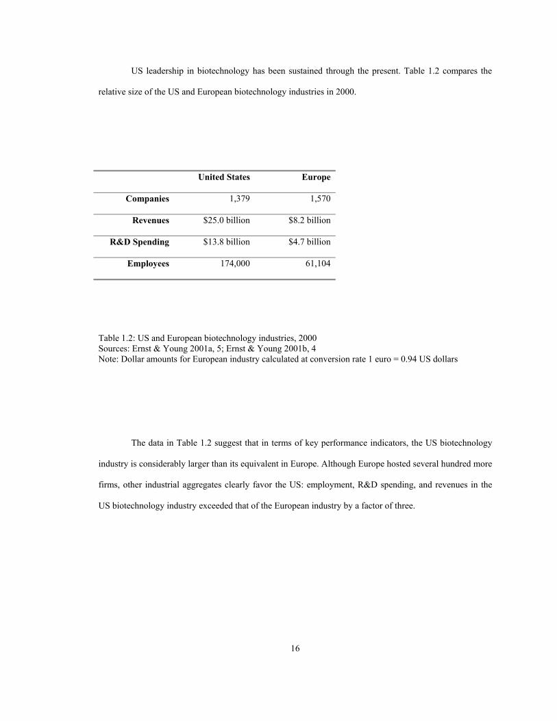
US leadership in biotechnology has been sustained through the present. Table 1.2 compares the
relative size of the US and European biotechnology industries in 2000.
United States Europe
Companies 1,379 1,570
Revenues $25.0 billion $8.2 billion
R&D Spending $13.8 billion $4.7 billion
Employees 174,000 61,104
Table 1.2: US and European biotechnology industries, 2000 Sources: Ernst & Young 2001a, 5; Ernst & Young 2001b, 4 Note: Dollar amounts for European industry calculated at conversion rate 1 euro = 0.94 US dollars
The data in Table 1.2 suggest that in terms of key performance indicators, the US biotechnology
industry is considerably larger than its equivalent in Europe. Although Europe hosted several hundred more
firms, other industrial aggregates clearly favor the US: employment, R&D spending, and revenues in the
US biotechnology industry exceeded that of the European industry by a factor of three.
16
The dominance of US biotechnology firms vis-à-vis the rest of the global industry is also
suggested by an examination of patenting trends in genetic engineering. Table 1.3 describes the distribution
of international patent families4 and highly-cited patent families5 in genetic engineering for selected
countries between 1990 and 1994.
Priority Country Patent Families (share of total)
Highly-Cited Patent Families (share of total)
United States 2,165 (64%) 23 (59%)
Japan 441 (13%) 4 (10%)
United Kingdom 344 (10%) 4 (10%)
Germany 244 (7%) 1 (3%)
France 196 (6%) 7 (18%)
Table 1.3: International patent families in genetic engineering (selected countries): 1990-1994 Source: National Science Board 1998, 6-28
4 A patent family “consists of all the patent documents published in different countries associated with a single invention. The first application filed anywhere in the world is the priority application: it is assumed that the country in which the priority application was filed is the country in which the invention was developed ... An international patent family is created when patent protection is sought in at least one other country besides that in which the earliest priority application was filed.” (National Science Board 1998, 6-23) 5 “Interpatent citations are an accepted method of gauging the technological value or significance of different patents. These citations, provided by the patent examiner, indicate the ‘prior art’ – the technology in related fields of invention – taken into account in judging the novelty of the present invention. The number of citations a patent receives from later patents can serve as an indicator of its technical importance or value.” (National Science Board 1998, 6-24)
17
The data in Table 1.3 indicates that not only was the US the source of much of the patenting
activity in genetic engineering during 1990-1994 (64 percent), it was also the country from which most of
the important (i.e., highly-cited) patents originated (59 percent). These results lend further credence to the
assertion that the US is indeed the world leader in biotechnology.
The limited amount of international trade in biotechnology-related products is also dominated by
the US. One source observes that “[t]he net US trade balance in biotech-related products, royalties for
technology licenses, and payments for contract R&D services is clearly positive. Most biotech-derived
products on the market are of US-origin. For example, the top-selling biotech-derived biopharmaceuticals,
the largest market component of the biotechnology industry, were developed by US companies and are
largely produced in the Unites States for export …” (Office of Technology Policy 1997, 102).
Estimates place the US share of world exports in biotechnology in 1994 at 37 percent, compared
to 17 percent for Japan, and 12 percent for Germany. An examination of the US trade balances in
biotechnology for the period 1990-1999 (Table 1.1) indicates that the US has achieved a surplus in
biotechnology trade throughout the period, rising over 50 percent from $629.1 million in 1990 to a peak of
$956.0 million in 1994, before falling to $587.8 million in 1999.
1.2.3 Biotechnology R&D Investment
The US Office of Technology Policy (1997, 10) observes that the “biotechnology industry is the
most research-intensive industry in civilian manufacturing”. This is largely because biotechnology is an
industry founded on the commercialization of leading-edge scientific knowledge. The management expert
Peter Drucker identifies seven sources of innovative opportunity; the “least reliable and least predictable” –
hence, the most difficult and uncertain to exploit – is “new knowledge” (Drucker 1985, 35-36). Formation
of the biotechnology industry was a response to perceived economic opportunities emerging from new
knowledge accumulating in molecular biology. While there is potential for extraordinary economic returns
in biotechnology, the R&D commitments necessary to realize them are sobering. “Biotechnology as an
industry continues to be characterized by high capital costs, treacherous regulatory barriers, and difficult
R&D hurdles.” (Teitelman 1994, 201)
18
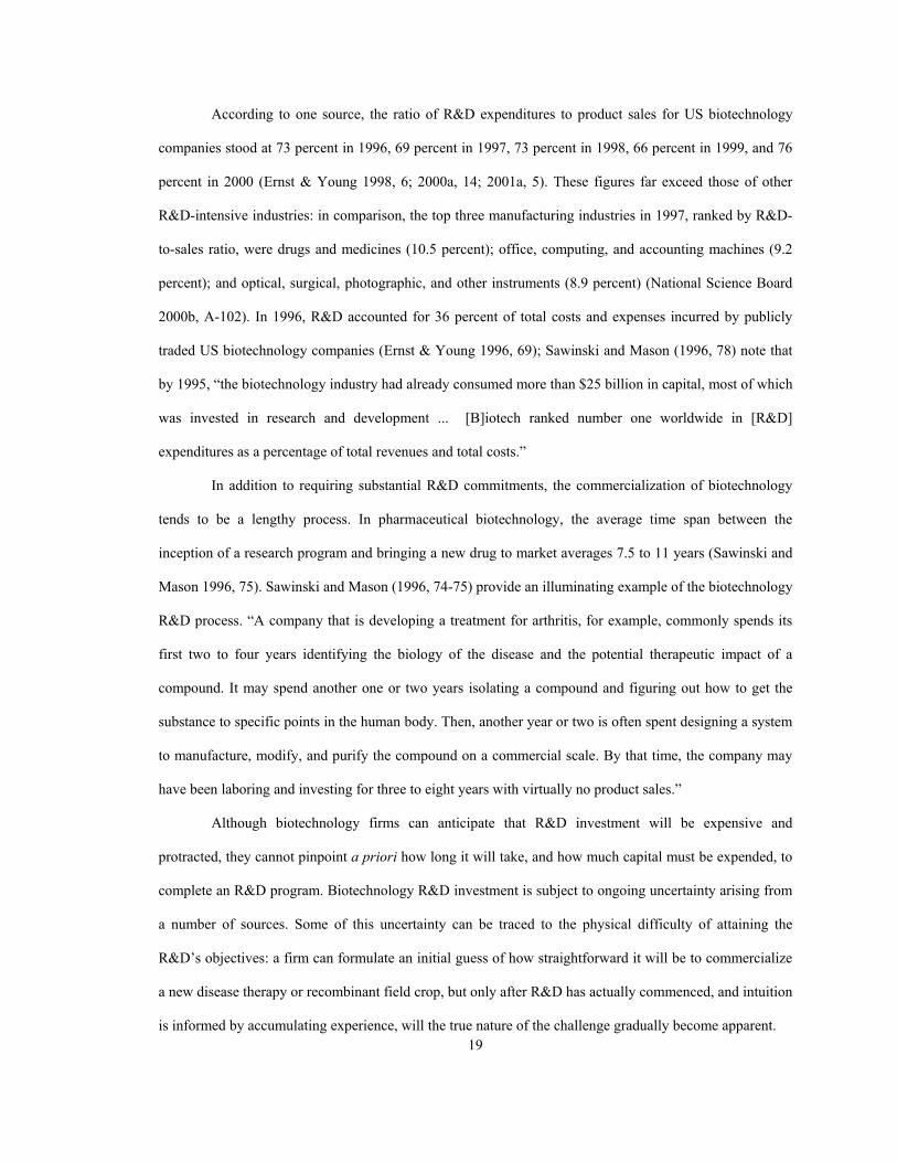
According to one source, the ratio of R&D expenditures to product sales for US biotechnology
companies stood at 73 percent in 1996, 69 percent in 1997, 73 percent in 1998, 66 percent in 1999, and 76
percent in 2000 (Ernst & Young 1998, 6; 2000a, 14; 2001a, 5). These figures far exceed those of other
R&D-intensive industries: in comparison, the top three manufacturing industries in 1997, ranked by R&D-
to-sales ratio, were drugs and medicines (10.5 percent); office, computing, and accounting machines (9.2
percent); and optical, surgical, photographic, and other instruments (8.9 percent) (National Science Board
2000b, A-102). In 1996, R&D accounted for 36 percent of total costs and expenses incurred by publicly
traded US biotechnology companies (Ernst & Young 1996, 69); Sawinski and Mason (1996, 78) note that
by 1995, “the biotechnology industry had already consumed more than $25 billion in capital, most of which
was invested in research and development ... [B]iotech ranked number one worldwide in [R&D]
expenditures as a percentage of total revenues and total costs.”
In addition to requiring substantial R&D commitments, the commercialization of biotechnology
tends to be a lengthy process. In pharmaceutical biotechnology, the average time span between the
inception of a research program and bringing a new drug to market averages 7.5 to 11 years (Sawinski and
Mason 1996, 75). Sawinski and Mason (1996, 74-75) provide an illuminating example of the biotechnology
R&D process. “A company that is developing a treatment for arthritis, for example, commonly spends its
first two to four years identifying the biology of the disease and the potential therapeutic impact of a
compound. It may spend another one or two years isolating a compound and figuring out how to get the
substance to specific points in the human body. Then, another year or two is often spent designing a system
to manufacture, modify, and purify the compound on a commercial scale. By that time, the company may
have been laboring and investing for three to eight years with virtually no product sales.”
19
Although biotechnology firms can anticipate that R&D investment will be expensive and
protracted, they cannot pinpoint a priori how long it will take, and how much capital must be expended, to
complete an R&D program. Biotechnology R&D investment is subject to ongoing uncertainty arising from
a number of sources. Some of this uncertainty can be traced to the physical difficulty of attaining the
R&D’s objectives: a firm can formulate an initial guess of how straightforward it will be to commercialize
a new disease therapy or recombinant field crop, but only after R&D has actually commenced, and intuition
is informed by accumulating experience, will the true nature of the challenge gradually become apparent.
Events external to the R&D process may also conspire to quicken or slow the pace of R&D. For
example, the regulatory regime governing the industry may impose unanticipated costs, in the form of
extended testing programs, or excessively complex or burdensome approval procedures for genetically
modified products. Consumer opinion, in the form of public perception of biotechnology, may also impact
the R&D process, most likely through ongoing uncertainty over the value of successfully completed R&D.
This factor is especially important in agricultural applications of biotechnology.
Finally, ongoing basic research, conducted either in the scientific community or by the firm itself,
may reveal that a current biotechnology commercialization effort is based on faulty scientific principles,
and is therefore untenable. A case in point is the effort to develop a drug therapy for sepsis, an infection
often encountered in cancer patients or burn victims. Numerous biotechnology companies collectively
invested hundreds of millions of dollars in R&D directed at developing a drug for sepsis. However, all of
the drugs failed, because it was later discovered that sepsis could not be easily treated with only one drug.
Since biotechnology R&D is in many instances little removed from basic research, this form of uncertainty
is likely to impact most efforts to develop biotechnology products.
The fact that biotechnology is based on incompletely understood living systems such as humans,
animals, and plants implies that R&D programs will be subject to ongoing variation in anticipated cost and
returns over the life of the investment. Success is far from assured: “many companies either never produce
a marketable product, or do not obtain regulatory approval.” (Sawinski and Mason 1996, 75) While
biotechnology firms that choose to leave the industry can sometimes sell their research to other firms,
finding a potential buyer and/or fully recovering past expenditures is by no means assured. Therefore, R&D
expenditures must be considered at least partially sunk.
1.3 STRUCTURE AND DYNAMICS OF THE BIOTECHNOLOGY INDUSTRY
20
Oehmke, et al. (1999, 4) note the “gross empirical regularity that the life science industry is
composed largely of two types of firms.” “The first type of firm,” the authors observe, “is the large,
multinational corporation with expensive but well-funded research in a variety of biotechnological areas ...
These ‘life science’ companies attempt to maximize profits by applying biotech to the historical
pharmaceutical, agriculture, and nutrition industries. The second type of firm is a small, start-up life science
firm. These firms often arise from the inspiration and discovery of a single or a small team of scientists ...”
(Oehmke, et al., 4). In this section, start-ups and multinationals are defined and discussed, leading up to a
description of the biotechnology industry dynamics which emerged as a result of the R&D investment
behaviors of each class of firm.
1.3.1 Start-ups
Start-up firms may be defined as business entities set up to exploit commercial opportunities in
emerging high technology industries. At the time of its inception, a start-up firm has no established product
lines or other revenue-producing assets; rather, the firm’s value is almost completely embodied in its
“knowledge capital” – ideas, skills, and other forms of proprietary human capital the firm’s principle
stakeholders believe can be translated into profit-making products and services.
As Oehmke, et al. (1999) point out, a start-up is often created by one or more “bench scientists”,
who typically conduct basic research in the science underpinning the technology. For example, Genentech,
one of the first biotechnology start-ups, was co-founded by Herbert Boyer, the scientist who pioneered
recombinant DNA. Calgene, the start-up which created the first genetically modified food approved by the
FDA, was co-founded by Ray Valentine, a University of California at Davis plant scientist. The skills and
knowledge of the start-up’s scientific talent account for much of the firm’s anticipated value.
Since a start-up has no internally-generated capital to fund the commercialization of marketable
products, it must rely on external financing to see the company through its formative years. Typically, this
involves a partnership with a venture capitalist. “Venture capitalists typically make investments in small,
young companies that may not have access to public or credit-oriented institutional funding. Venture
capital investments can be long term and high risk, and may include hands-on involvement by the venture
capitalist in the firm. Venture capital thus can aid the growth of promising small companies and facilitate
the introduction of new products and technologies, and is an important source of funds used in the
formation and expansion of small high-technology companies” (National Science Board 2000a, 7-23).
21
The financial evolution of a start-up firm from creation to maturity can be characterized as the
“inception – venture capital – IPO” cycle. After a company's formation, venture capital finances the firm's
activities until it is sufficiently developed to warrant an initial public offering (IPO) on the equity markets.
At this point, the venture capitalist will usually liquidate its stake in the start-up, in the hopes of reaping a
substantial return on its original investment. A key requirement for a well-functioning venture capital
industry is the existence of equity markets willing to purchase the IPOs, thus providing liquidity for the
venture capitalist's investment. In 1980, the IPO of Genentech, the first by a biotechnology company, set a
Wall Street record as the initial share price of $35 rose to a peak of $89 on the first day of trading. The
success of Genentech sparked a flurry of offerings by other biotechnology start-ups.
Future success of the start-up depends on the continued willingness of the capital markets to
provide funds. For example, Calgene, in an effort to secure funding necessary for, among other things, the
commercialization of the Flavr-Savr tomato, registered a stock offering of two million shares in September
1994. (Investor’s Business Daily 1994, A6). But the use of external financing sources – in particular,
venture capital and the equity markets – is attended by a number of disadvantages, chief among them being
that the start-up is often held hostage to the whims of investor sentiment. This sentiment can reflect
investors’ confidence in the future profitability of the underlying technology, but may also be a function of
the relative popularity of one high technology industry vis-à-vis other high technology industries. In 2000,
venture capital disbursements rose to an all-time high of nearly $1.3 billion, yet the share allocated to
biotechnology firms hit an all-time low that same year, coinciding with the Internet boom of that period.
The data in Table 1.4 indicates that venture capital investments in biotechnology have followed a “boom or
bust” pattern, both in absolute terms and as a percentage of total disbursements.
22
Year All Industries Biotechnology(share of total)
Year All Industries Biotechnology (share of total)
1980 11.0 1.1 (10%) 1991 88.0 6.8 (7.7%)
1981 47.7 2.3 (4.9%) 1992 158.2 49.9 (31.5%)
1982 63.1 1.6 (2.5%) 1993 314.2 44.8 (14.3%)
1983 111.4 5.3 (4.8%) 1994 236.7 46.7 (19.7%)
1984 129.7 10.4 (8.0%) 1995 312.5 9.4 (3.0%)
1985 103.9 6.2 (5.9%) 1996 376.8 42.5 (11.3%)
1986 117.6 13.7 (11.7%) 1997 629.3 68.1 (10.8%)
1987 122.0 15.6 (12.8%) 1998 717.1 85.6 (11.9%)
1988 144.4 26.0 (18.0%) 1999 710.7 44.4 (6.3%)
1989 184.8 53.2 (28.8%) 2000 1,282.8 11.7 (0.9%)
1990 124.6 7.5 (6.0%)
Table 1.4: US venture capital disbursements: 1980-2000 (millions of dollars) Source: National Science Board 2002, A6-66
1.3.2 Multinationals
Multinational corporations are well-defined entities within economic theory and the literature. For
the purposes of this study, the conventional interpretation of a multinational is adopted; a classic reference
is Caves (1982), who defines a multinational as “an enterprise that controls and manages production
establishments – plants – located in at least two countries” (Caves, 1).
23
Multinationals engaged in biotechnology are broadly associated with the pharmaceutical or
chemical industries. Examples include Monsanto, Eli Lilly, and Hoffman-LaRoche. However, these
multinationals typically exhibit a high degree of horizontal conglomeration, making industry classification
difficult: for example, the product line of Swiss-based Novartis includes contact lenses, baby food, animal
health care, and human pharmaceuticals.
Ownership of a diversified portfolio of established, revenue-generating product lines implies that
multinationals will, in general, have access to reserves of internally generated capital to at least partially
fund biotechnology R&D investment. The fact that multinationals are less dependent than start-ups on
external capital markets to fund R&D activity may lessen the imperative for multinationals to initiate and
expedite the biotechnology commercialization process. This in turn expands the range and flexibility of
potential R&D investment strategies for multinationals, an issue which will be addressed later in this study.
1.3.3 Industry Dynamics
The following discussion is based on Sharp (1996) and Senker, Joly, and Reinhard (1996).
Biotechnology has undergone three phases. The first phase involved the use or manipulation of live
organisms in centuries-old forms of production: e.g., cross-breeding of livestock, hybridized plants, or the
use of live yeast in brewing or baking. The second phase, beginning in the early part of the 20th century,
involved the use of micro-organisms in various production processes: in particular, the use of enzymes to
produce useful substances. Finally, the third stage, initiated circa 1970, is based on breakthroughs in
molecular biology, and in particular, the use of recombinant DNA techniques in the agricultural and
pharmaceutical sectors.
Scientific advances in molecular biology, and in particular, the results of Boyer and Cohen,
initiated the formation of biotechnology start-ups. As Sharp (1996, 3) observes, the emergence of the
biotechnology start-up company was primarily a US phenomenon. The successful IPO of Genentech in
1980 was a prelude to the formation of numerous US biotechnology start-ups in the early 1980s, as the
industry expanded rapidly. Start-ups appeared in other countries as well, although not to the extent
witnessed in the US.
24
Early commercialization of biotechnology was performed almost exclusively by start-ups. The
multinational chemical and pharmaceutical companies, while recognizing that biotechnology had the
potential to yield new high-end products, nevertheless were hesitant to engage in full-scale biotechnology
commitments at the earliest opportunity. Rather, they adopted a “wait and see” strategy, preferring to
obtain more information on whether biotechnology would prove to be a viable technology. Therefore,
during the industry's early stages, the multinationals engaged in only limited biotechnology investments.
This “minimalist strategy” involved the creation of small-scale in-house biotechnology research facilities,
“large enough to keep abreast of the science and to monitor developments and competitors” (Sharp 1996,
11).
The multinationals also placed small research contracts with the start-ups, often for as little as $1 -
5 million. “In this essentially contract research role,” Sharp (1996, 4) notes, “the [start-ups] performed two
very useful functions. Firstly, they acted as intermediaries between the large companies and the academic
base. Because of close academic links they were able quickly to put together the cross-disciplinary teams
required to develop new products in this new technology, whereas the big firms, with their traditional
contacts in chemistry not biology departments, found it difficult to find the right people … Secondly, they
enabled the large companies to hedge their bets. Research contracts for $1m, $2m even $5m were limited
commitments which might yield substantial prizes but, at a minimum, would provide the contractor (i.e.,
the large company) with useful research results and avoid long-term and expensive employment
commitments at a time when it was still uncertain where biotechnology was going.”
Sharp observes that by the mid-1980s, “the period of watching and waiting was over. Most of
these large companies recognized that, whatever their original reservations, biotechnology had established
itself as an important enabling technology (i.e., a route to new product development) and would be
essential for future product innovation” (Sharp, 12). Multinationals now entered into major biotechnology
commitments: building up in-house resources, entering into R&D and licensing agreements with start-ups,
or even acquiring them outright. The formation of start-up/multinational combinations, either through
arms-length agreements or acquisition, is a process which extends to the present, evidenced by a relatively
continuous process of strategic alliance-making and consolidation.
25
The interaction between start-ups and multinationals is of particular interest in biotechnology. The
industry’s transition from one populated mainly by start-ups to one including multinationals as well was
characterized by a transfer of assets from the former to the latter. “Most [start-up] biotechnology companies
... raised capital to perform fundamental research years before commercialization began and profits came.
Few were able to generate financing to fund an entire product cycle at once, and so they continually
returned to Wall Street, begging bowl at ready, often to discover that investors had turned against high-risk
ventures just when they needed the help the most. Failing to raise money by selling equity, these firms were
forced to auction off assets (from product licenses to the company itself, depending on their plight ... The
result was that the established drug companies received the fruits of the first decade of biotechnology by
simply waiting for the money to run dry. New products fell into their laps” (Teitelman 1994, 197-198). In
summary, the start-ups pioneered the biotechnology industry via the scientific expertise they recruited to
their organizations; the multinationals, on the other hand, were later entrants, often benefiting from access
to the proprietary knowledge stocks accumulated by the start-ups during the first ten years of the industry.
1.4 STYLIZED DESCRIPTION OF BIOTECHNOLOGY R&D INVESTMENT
Romer (1989, 53-54) paraphrases an important insight from the eminent theorist Nicholas Kaldor:
“[A] theorist ought to start with a summary of the facts that are relevant to the problem of interest. This
summary should be ‘stylized’, ... concentrating on broad tendencies. In the formative stages of a body of
theory, this kind of informal treatment of the data can be quite useful, for without stylized facts to aim at,
theorists would be shooting in the dark.”
26
In this spirit, a set of stylized facts describing the salient characteristics of R&D investment in the
biotechnology industry are listed below. Given the exceptionally high degree of R&D intensity prevailing
in the biotechnology industry, it is likely that analysis of biotechnology firms’ economic decision-making
must account for the process by which resources are committed to R&D. In light of this, the stylized facts
serve a dual role. First, they constitute a benchmark by which existing theories can be evaluated in terms of
their relevancy to the biotechnology industry. Second, if existing theories are found wanting, the stylized
facts represent a summary of the key elements of biotechnology R&D investment for which new theories
should account.
STYLIZED FACTS OF BIOTECHNOLOGY R&D INVESTMENT
• R&D costs are at least partially irreversible: i.e., the costs of unprofitable R&D cannot be fully recovered
• R&D cost is upfront: i.e., R&D must be successfully completed before any return on investment is realized
• R&D is lengthy: i.e., it cannot be completed in one time period. However, time to build is unknown a priori
• The cost to complete an R&D program is subject to three forms of ongoing uncertainty:
- the physical difficulty of completing the R&D - the external investment environment - the scientific environment
This uncertainty can be resolved gradually over time as investment is sequentially completed. However, total R&D cost is not known with certainty until the R&D is completed.
The remainder of this study reflects the maintained hypothesis that these stylized facts provide a
sufficient characterization of the biotechnology R&D investment process to motivate and analyze the
economic questions posed in the next section.
1.5 TWO ECONOMIC QUESTIONS
The empirical description of the biotechnology industry presented in this Chapter suggests two
economic questions:
• Why did the United States emerge as the world leader in biotechnology, vis-à-vis other Northern countries?
• Why did start-ups, on average, enter the biotechnology industry prior to multinationals?
The first question is motivated by the most fundamental issue in international economics: a
description of the primitive elements that account for the pattern of specialization and trade observed in the
international economy. In the context of the present study, this issue can be framed as the identification of
the source of the US comparative advantage in biotechnology.
The second question is concerned with the industrial structure of commercial biotechnology, with
an emphasis on how that structure has evolved over time, and by what mechanisms evolution was achieved.
It is evident that two classes of economic agents, start-ups and multinationals, responded with different
behaviors when faced with the opportunity to invest in biotechnology R&D. What incentives were
determinative in forming these asymmetric investment strategies?
The remainder of this study articulates, models, and analyzes the implications of these questions.
27
CHAPTER 2
COMPARATIVE ADVANTAGE AND DYNAMICS IN HIGH TECHNOLOGY INDUSTRIES
It is useful to survey the existing literature to assess its relevance to the economic questions posed
at the end of Chapter 1. Comparative advantage is the fundamental principle of international economics,
and is therefore an appropriate starting point for considering the two economic questions. The intuition of
this concept is discussed in Section 2.1. Comparative advantage has been extended beyond its basic
expressions in the Ricardian and Heckscher-Ohlin-Samuelson formulations. The main strands of this
literature – imperfect competition, “history matters”, and endogenous innovation – are discussed in Section
2.2. Endogenous innovation is the extension most relevant to high technology industries like
biotechnology; Grossman and Helpman’s (1991e) widely-cited exposition of this theory is reviewed in
Section 2.3. The Chapter concludes in Section 2.4 with an evaluation of the Grossman and Helpman
framework’s utility in answering the two economic questions.
2.1 COMPARATIVE ADVANTAGE
28
One of the most elegant and non-obvious results in economic theory is the principle of
comparative advantage, developed by Ricardo (1817) in The Principles of Political Economy and Taxation.
Smith (1776) introduced the proposition that nations trade in order to exploit absolute differences in
autarkic prices. Ricardo’s deep insight was that this proposition can be generalized to the case where
bilateral absolute advantages do not exist. In these circumstances, differences in relative autarkic prices are
sufficient to generate incentives for specialization and international trade, even when one country exhibits
lower marginal costs across all industries. Ricardo elucidated a general proof of the benefits of free
exchange that applied equally well to any class of economic agent, whether individual, firm, or nation.
Although comparative advantage eventually was formalized as a property of the neoclassical general
equilibrium, and, therefore, as a feature of free exchange at any level of aggregation, it was, as Findlay
(1991, 99) points out, “in the context of international trade that [it] was discovered and has been
investigated ever since.”
Comparative advantage is derived from the existence of heterogeneity in the international
economy. Cross-country asymmetries in the endowment of a “primitive element”, or basic characteristic of
the open economy, are reflected in international differences in relative marginal cost, which in turn create a
corresponding asymmetry in autarkic prices. Pre-trade international price differences form the incentive for
a Pareto-improving re-allocation of world-wide production, realized through specialization and free
exchange. The primitive element driving this process is usually identified as one of the exogenous
components of the general equilibrium: i.e., production technologies, factor endowments, or consumer
preferences. While the last case is not theoretically interesting6, the remaining two serve as the fundamental
axioms for the Ricardian and Heckscher-Ohlin trade theories. In orthodox positive trade theory, the
definition of the primitive element which organizes comparative advantage constitutes an irreducible
description of the determinant of the pattern of international trade.
2.2 INTERPRETATIONS OF COMPARATIVE ADVANTAGE
2.2.1 The Factor Proportions Theory
Comparative advantage is most widely understood in terms of the factor proportions model,
originally conceived by Heckscher (1919), and refined by Ohlin (1933) and Samuelson (1948, 1949, 1953).
The factor proportions model ascribes international differences in relative autarkic prices to an asymmetric
distribution of productive factors across countries. The two-factor, two-good, two-country exposition of
this theory yields a number of well-known properties. The Heckscher-Ohlin theorem identifies the cross-
country pattern of relative factor endowments as both the source of comparative advantage and the
determinant of international trade: a country possessing a relative abundance of a particular factor will tend
6 See Dixit and Norman (1980, 3). The authors note that the triviality of consumer preferences as a basis for trade applies to the case of competitive equilibrium trade models; preferences can assume a more prominent role in models that incorporate imperfect competition and product diversity.
29
to specialize in the production and export of the good using that factor relatively intensively in its
production. Specialization and exchange among countries eliminates the difference in pre-trade prices by
shifting global production until all opportunities for welfare-improving re-allocations are exploited. The
factor price equalization theorem states that as each country increases production of the good for which it
possesses a comparative advantage, the price of its abundant factor will also increase until factor prices are
equalized across countries; at this point, incentives for further re-allocations are exhausted.7
The 2x2x2 factor proportions model yields several additional results. The Stolper-Samuelson
theorem states that an increase in the price of one good, holding the other constant, will raise the return to
the factor used intensively in its production by a proportion greater than the price increase, while causing
the return to the second factor to fall. The Rybczynski theorem postulates a similar relationship between
changes in factor supplies and the production of each good.
Several studies have tested the robustness of the 2x2x2 model’s properties to generalizations over
the dimensionality of output and factors. Neary (1985) demonstrates that the Stolper-Samuelson and
Rybczynski theorems can be weakly approximated in higher-dimensional models using index number
theory. Jones and Scheinkman (1977) find that factor intensity and the factor proportions theory can be
generalized to higher dimensions. In terms of the Stolper-Samuelson and Rybczynski theorems, they
conclude that the magnification effect does generalize in the case of the former; the Rybczynski result, on
the other hand, is sensitive to the relative number of goods and factors and generalizes only to the extent
that given an increase in the supply of one factor i, there exists a sector j which will contract.8 In both cases,
generalization is contingent on the assumption of no joint production.
While the factor proportions model fares well in explaining North-South trade – i.e., trade between
industrialized countries and the developing world – it tends to break down in the face of two empirical
observations of the post-1945 period: 1) trade between industrialized nations expanded steadily, and 2)
7 This theorem is obtained under the assumption that the difference in per-unit capital/labor requirements between the two goods is greater than the difference in capital/labor endowment ratios between the two countries. 8 Jones and Scheinkman summarize this generalized Rybczinski effect by postulating that every industry has some “natural enemy” among the set of productive factors.
30
industrialized nations were converging in terms of most economic measures, including factor proportions
(Helpman and Krugman 1985, 2). These observations contradict the intuition of the factor proportions
interpretation of comparative advantage.
Empirical tests of the factor proportions model cast further doubt on the relevancy of its
assumptions to trade between Northern nations. The classic reference is Leontief (1953), whose famous
paradox found that the US, though capital-abundant, nevertheless exported goods embodying more labor
than its imports. Another empirical study by Bowen, Leamer, and Sveikauskas (1987) used data from 1967
to test the theoretical proposition that a country’s exports should embody factors for which its share of the
world endowment exceeds its share of world income. They determined that for two-thirds of the factors,
trade followed the Heckscher-Ohlin pattern for less than 70% of sampled countries.
A study by Trefler (1993) offers some support for the factor proportions theory. A common
criticism of factor proportions is that factor price equalization is rarely observed empirically. Trefler noted
that cross-country differentials in factor productivity would cause absolute measures to understate the size
of the labor force in relatively productive countries, and overstate it in relatively unproductive ones.
Furthermore, workers who are twice as productive should expect to receive a wage twice that of labor in
other countries. Trefler tested his hypothesis using the Heckscher-Ohlin-Vanek (HOV) result that the factor
content of a nation’s net exports should reflect the factor in which it is relatively abundant. He found that a
“close correspondence” did appear to exist between relative factor prices and the relative productivity
estimates, lending support to “an HOV model that allows for factor-augmenting international technology
differences and the implied international factor price differences” (Trefler, 973)
Trefler speculates that international differences in productivity parameters may reflect a country’s
ability to assimilate and exploit new technologies. “One facet of national differences ... is the ability to
commercialize technology. While basic research is internationally available through publications of the
scientific community, the translation of basic research into low-cost production processes is both a guarded
secret of firms and the comparative advantage of the developed countries.” (Trefler, 980)
31
The emergence of the US as the world leader in biotechnology suggests that Trefler’s statement
might be amended to say that the ability to translate science into commercial technology appears to be the
comparative advantage of some developed countries, vis-à-vis other developed countries. Determining why
this is so is the focus of the first economic question posed in Chapter 1.
2.2.2 Beyond Factor Proportions
In the last two decades, international trade theory has been invigorated by fresh appraisals of some
of the most fundamental issues, with an emphasis on bridging the gap between theory and evidence. The
apparent failure of the factor proportions theory to explain the empirically observed pattern of
specialization and trade between industrialized nations has led to new interpretations of comparative
advantage. This new literature has emerged largely from the interface of two economic sub-disciplines:
international trade and industrial organization. International trade theorists have looked beyond the standard
general equilibrium model of perfect competition to explore new theories of comparative advantage based
on more granular industrial processes and characteristics than had been addressed in the past.
Krugman (1990) identifies four major themes which have emerged in the literature. First,
economists have re-opened the question of what causes international trade. Recognition that many global
markets fall short of the perfect competition benchmark led some theorists to examine the effect of
increasing returns to scale on the pattern of specialization and trade. A corollary to this work – strategic
trade policy – re-examines the efficacy of trade policy, given that markets are imperfectly competitive.
Another strand of the literature, attributable to Krugman himself, explores the role of history in determining
comparative advantage: an initial, possibly random, pattern of specialization can become permanent
through accumulating economies of scale, particularly external economies. Finally, a class of models
examines the issue of technology and international trade, departing from traditional models by tracing not
only the effect of technology on trade flows, but also probing the sources of technological asymmetries
across nations. The key point of this literature is that R&D must be represented as an endogenous process
in industries like biotechnology where innovation assumes a prominent role.
32
2.2.2.1 Increasing Returns to Scale and Product Differentiation
If the standard assumption that markets are perfectly competitive is suspended, new incentives for
international trade emerge, even among relatively similar trading partners. Increasing returns to scale can
create a comparative advantage, albeit an arbitrary one, for the country which realizes efficiency gains
through large scale production. Differentiated products also provide an incentive for similar countries to
trade among themselves, regardless of the lack of other fundamental asymmetries.
Krugman (1979, 1980, 1981a) explores the consequences of increasing returns to scale in an open
economy characterized by monopolistic competition. He demonstrates that even in the case of identical
countries, incentives for trade can arise through an expansion of the market and a simultaneous realization
of economies of scale. This result echoes Smith’s (1776, 121) original rationale for a division of labor: “As
it is the power of exchanging that gives occasion to the division of labor, so the extent of this division must
always be limited by the extent of that power, or, in other words, by the extent of the market.” In addition
to the gains realized from scale economies, consumers benefit from an expansion in the range of products
available, which, because of the assumption of increasing returns, is necessarily limited under autarky.
Product differentiation represents another incentive for similar countries to establish mutually
beneficial trade relations. Two approaches capture this effect: consumers can possess a “love of variety”
(Krugman (1980), Helpman and Krugman (1985)) within a particular class of good, or alternatively,
consumers can adopt a bundle of characteristics as their “ideal variety” (Lancaster (1980), Helpman
(1981)). In either case, economies of scale dictate that only one country will produce a given variety, and
two-way trade in similar, yet differentiated goods will arise between countries not otherwise
distinguishable on the basis of factor endowments or technology. Gains from trade are realized through an
expansion of the available varieties of a particular good, which, by construction of preferences, directly
increases the welfare of consumers in both countries.
33
Models of increasing returns to scale and product differentiation provide a theoretical basis for
trade between similar countries, but a number of criticisms have been levied against this approach. Chief
among them is that within this class of models, trading equilibriums tend to be arbitrary; as a result,
comparative advantage becomes a consequence of random circumstance. Despite this limitation, trade
models with imperfect competition derive incentives for international trade based on real-world
characteristics of market structure.
2.2.2.2 Strategic Trade Policy
One of the most emphatic implications of the orthodox theories of international trade is that the
unimpeded flow of goods and services across national borders is, in nearly all circumstances,
unambiguously welfare-improving. However, once the possibility of imperfect competition, and thus super-
normal profits, is introduced, this assertion loses much of its impact. Indeed, persuasive arguments can be
made that the presence of imperfectly competitive markets necessitates government policy intervention.
The classic reference is Brander and Spencer’s (1984, 1985) series of papers on the potential for
profit-shifting which exists in imperfectly competitive international markets. Brander and Spencer point out
that if an industry is oligopolistic, governments can shift profits to domestic firms at the expense of foreign
rivals through the use of policies such as export subsidies or tariffs. This form of intervention creates an
advantage for home firms and eliminates the arbitrary nature of the trading equilibrium: production can be
unambiguously located in the home country, along with the corresponding profits.
34
Despite the theoretical clarity of the Brander-Spencer framework, a number of studies have
exposed weaknesses in its practical implementation, e.g. Grossman (1986), Grossman and Richardson
(1985), and Eaton and Grossman (1986). The most glaring limitation is the sensitivity of the model to its
underlying assumptions. Policymakers must have specific information on the type of oligopolistic game
firms are playing – i.e., Cournot or Bertrand – in addition to legitimate evidence that the industry is indeed
imperfectly competitive. Policy responses from foreign governments whose client firms are targeted by
strategic trade policies can erase any initial welfare improvements in a steadily escalating battle of
protectionist intervention, a possibility that Brander and Spencer recognized. Furthermore, strategic trade
policies which expand the production of one industry can have deleterious general equilibrium effects on
other industrial sectors, bidding up the price of scarce factors to prohibitive levels.
In conjunction with the literature associated with economies of scale, Krugman (1984) suggests
that protection of the domestic market might be a form of export promotion: freeing the home market from
foreign competitors could allow oligopolistic domestic firms to achieve lower costs through economies of
scale or movement down the learning curve. This cost advantage can then be translated into a competitive
advantage in export markets. This model departs from those which employ scale economies as an incentive
for trade in that the benefits here are one-sided: only one country achieves the necessary scale of production
to realize efficiency gains, and these benefits are achieved by crowding out its competitors.
While strategic trade policy has attracted the interest of a number of economic theorists, most are
quick to point out that their models are not an avocation of a protectionist policy regime. Referring to
misguided implementation of strategic trade theories, Krugman (1986, 19) notes that the authors of these
models “have been surprised and perhaps worried at the places they find themselves cited.”
2.2.2.3 The Role of History
A less visible offshoot of the increasing returns approach to international trade is a small class of
models in which an arbitrary pattern of specialization can be established permanently as economies of scale
accumulate. Krugman (1981b, 1987) is again a path-breaking contributor, although some intellectual debt
is owed to Ethier (1982) for his work related to external economies and international trade. The premise of
these models is that an initial division of labor among countries, possibly established on the basis of a
Ricardian or Heckscher-Ohlin asymmetry, or even by accident, can be self-perpetuating over time: thus, in
Krugman’s words, “history matters”.
In Krugman’s earlier paper, such a model is employed to shed insight on the phenomenon of
uneven development: why does the distribution of income among the world’s economies tend to be
polarized between rich and poor nations? Krugman demonstrates that a nation with a head start in
producing a good subject to external economies will eventually crowd out the corresponding industrial
sector of its trading partner. This uneven development will be reinforced over time, driven by higher profit
rates in the leading country, which in turn fuel more capital accumulation and growth.
35
Trade models which emphasize the role of history are used to explain such economic oddities as
why the world’s aircraft manufacturing center is located in Seattle, Washington: initial conditions, possibly
chance, located it there, and increasing returns reinforce and perpetuate this result. More generally, such
models indicate that beyond establishing an incentive for trade, increasing returns represent a powerful
advantage for certain industries and nations, and once achieved, strengthen a nation’s presence in a global
market over time. If increasing returns are a prevalent feature of the international economy, governments
have a strong motivation to undertake policies that establish initial conditions favorable to domestic firms.
2.2.2.4 Technology and Trade
The fourth and final theme Krugman (1990) identifies concerns the role of technology and
technological change in international trade. While economists have long recognized the importance of
technology in modeling international trade, it is only recently that they have addressed the attendant issue
of what causes differences in technology across nations. Treatment of this issue requires trade theorists to
modify their interpretation of the source of comparative advantage: in particular, the notion that
comparative advantage is derived from an exogenous endowment must be abandoned in favor of attributing
it to the outcome of an endogenous economic process.
The idea that the pattern of specialization is a consequence of explicit economic decision-making,
rather than an exogenous property of the economic system, is germane to both economic questions posed in
Chapter 1. In high technology industries like biotechnology, the economic process that is determinative in
shaping both comparative advantage, market structure, and industry dynamics is R&D investment. A class
of open economy models predicated on this theme has recently emerged. The models examine the pattern
of specialization and trade in high technology industries where the long-run trade equilibrium is a function
of each country’s allocation of resources to R&D. Models of this kind represent the segment of the new
trade theories most relevant to the economic questions. In the next two sections, a theoretical framework
that serves as the foundation of much of the work in this area is reviewed, and then evaluated in the context
of its relevancy toward answering the economic questions.
2.3 DYNAMIC OPEN ECONOMIES WITH ENDOGENOUS INNOVATION
2.3.1 Innovation as an Endogenous Process
36
The international economy is the composite of a hierarchical arrangement of subsystems: a set of
national economies, each of which can be decomposed into individual industries, which in turn can be
decomposed into economic agents – consumers, firms, etc. – which can be further decomposed into a
collection of processes – utility maximization, production, R&D, and so on – which operate on a set of
primitive resources – e.g., preferences or factor endowments. The decision-making and interaction of these
subsystems collectively produces the complex system represented by the world economy.
A fundamental issue in the construction of a theoretical formulation of a complex system like the
world economy is to determine which subsystems will be explicitly represented, and which will be stylized
as an exogenous parameter, or ignored. In high technology industries like biotechnology, a key sub-system
is the process of innovation, or R&D. An extensive literature, pioneered by Schumpeter (1942) and Arrow
(1962), see also Dasgupta and Stiglitz (1980), details the economic incentives to allocate scarce resources
to the development of new technologies, reinforcing what casual observation indicates: profit-maximizing
firms devote considerable resources to innovative activity. It is this activity that, in the aggregate,
determines a country’s technological capacity.
Economic theorists historically have placed the engine of technological change beyond the control
of the economic agents in their models. Schmookler (1966) notes “For some economists, this assumption
[of exogenous technological change] is only a methodological convenience; for others, it is a matter of
conviction. But few have given the question serious thought. While it drastically simplified the analysis of
traditional problems, the assumption also relieved the profession of any sense of obligation to explain
technological change.” Schumpeter (1942, 110) observes that “[i]t is quite wrong ... to say, as so many
economists do, that capitalist enterprise was one, and technological progress a second, distinct factor in the
observed development of output; they were essentially one and the same thing or, as we may also put it, the
former was the propelling force of the latter.”
37
Criticism of the assumption of exogenous technology can be extended to the theory of
international trade. The need to deepen theoretical descriptions of technology in international trade models
is well documented in the literature. Krugman (1990, 7) observes that while international trade theory has
dealt extensively with the implications of technological change, it has little to say about its causes.
Grossman and Helpman (1991e, 177) note that models which posit international differences in production
technologies as the source of comparative advantage are of limited use in understanding the pattern of
specialization, “because they fail to explain why countries have come to acquire technological supremacy
in a certain set of goods.” Grossman (1992, 10) notes the inadequacy of conventional trade theory in terms
of predicting future patterns of technological differences across countries: “Due to the static nature of the
notion of comparative advantage that underlies much of traditional thinking about trade, the theory has
been of little use in analyzing the evolution of trade patterns over time.”
The central thesis of models of international trade with endogenous innovation is that innovative
activity is undertaken by profit-maximizing economic agents, rather than by the altruistic “scientific
community” to which exogenous technological change is typically attributed. Firms that innovate
successfully either expand the variety of available products (horizontal product differentiation), improve
the quality of existing products (vertical product differentiation), or lower the per-unit cost of existing
products. In each case, R&D investment offers the potential for supernormal returns, and in a broader
context, transforms comparative advantage into an ongoing process of global technological competition.
Since biotechnology is an R&D-intensive industry, analysis of the pattern of specialization,
market structure, and dynamics in this industry should begin with a review of the international economics
literature that provides an explicit treatment of the R&D process. This literature is an offshoot of the
broader endogenous growth literature, which represents innovation as an endogenous process in its own
right. The driving principle behind endogenous growth theory is that “innovation [is] a distinct economic
activity with distinct economic causes and effects” (Aghion, et al. 1998, 1). The work of Solow (1956) and
others demonstrated that technological change was an important contributor to the rate of economic growth.
Representation of innovation as an endogenous process establishes a bridge between factors such as market
structure, trade, and government policy on the one hand, and long-run economic growth on the other,
through the effect of the former on the incentives to innovate. Aghion, et al. (1998) provide a synthesis of
the endogenous growth literature and its applications in various domains.
Much of the work in the area of endogenous innovation and international trade finds its
antecedents in the contributions of Grossman and Helpman (1990, 1991a, b, c, d, e). Indeed, many recent
contributions are self-described as either generalizations of the Grossman and Helpman approach, e.g.,
Taylor (1993), or closely related to their work, e.g., Dinopoulos, Oehmke, and Segerstrom (1993). Since
their work forms the foundation for much of the current theory, this study focuses on Grossman and
Helpman’s approach to modeling endogenous innovation in the context of dynamic open economies.
38
2.3.2 Endogenous Innovation with International Technology Spillovers
In a series of papers culminating in a book-length treatment, Grossman and Helpman develop a
class of international trade models in which comparative advantage and economic growth are driven by
continuous innovation. The central thesis of this work is that technological progress “results from
intentional industrial innovation, that is, from the allocation of resources to research and other information-
generating activities in response to perceived profit opportunities.” (Grossman and Helpman 1991e, 6)
Private innovation directly impacts the relative technological status of each country in the global economy,
which in turn fixes the pattern of specialization and trade. The deep insight is that comparative advantage is
not defined statically by inherited endowments, but rather by an on-going, dynamic process of endogenous
innovation; as Grossman and Helpman observe, “the momentary technological advantages that induce a
particular pattern of trade have more fundamental, dynamic determinants.” (Grossman and Helpman 1991e,
177)
Grossman and Helpman9 consider an open economy populated by two “large” countries, A and B,
each endowed with two productive factors: skilled and unskilled labor. Two production sectors exist in
each country: a homogeneous traditional good with a constant-returns-to-scale (CRS), time-invariant
technology, and a continuum of differentiated high-technology goods, using a CRS technology which
evolves dynamically through the intentional allocation of resources to innovation. The three economic
activities – R&D, and production in each of the two sectors – are distinguished by their relative factor
intensity: R&D is the most skilled-labor intensive, while production of the traditional good is the least.
Consumer preferences are identical across countries, and are constructed to reflect either a “love of
variety”, or to account for quality differences.10
9 The following discussion is adapted from Grossman and Helpman (1991e), Ch. 7. 10 For a complete discussion of product differentiation, see Beath and Katsoulacos (1991).
39
The model of horizontal product differentiation is discussed here. Consumers maximize
where pi is the price of a high technology good in country i, ni is the number of varieties of the high
technology good produced in country i, and ε is the constant elasticity of substitution between any two
varieties. Note that profits decline as the number of varieties available in either country increases.
A critical assumption is that new scientific information flows freely over national borders: i.e.,
there are perfect knowledge spillovers. Specifically, there exists a stock of knowledge capital Kn from
which researchers in both countries draw. Kn grows proportionately to the number of varieties of the
differentiated good available worldwide. The cost of inventing a new variety of the high-technology good
is the factor cost of research in each country divided by the knowledge stock: therefore, research costs fall
as Kn increases. Choosing units so that the knowledge stock equals the number of varieties in the world
economy, free entry requires that the capital market value of each firm equals the cost of inventing a new
good:
vi = cRi / n (5)
where vi is the market value of a firm located in country i, and cRi / n is the cost of developing a new variety
in country i given that n varieties already exist in the world economy.
Firms issue securities in order to finance their R&D programs; these securities are purchased by
consumers in order to smooth expenditures over time. The absence of arbitrage implies that each security
must earn a normal return:
πi + ∂vi/∂t = rivi (6)
In the steady state with a worldwide interest rate r = ρ, Equation 6 can be rearranged to give:
πi/vi = ρ + g (7)
where g = (∂n/∂t)/n is the rate of new product development in the world economy.
41
In a steady-state equilibrium in which both countries innovate, all goods and factor markets clear,
factor prices are constant, and the value of innovating firms declines at the rate of new product
development. The allocation of resources in each country across R&D, the traditional sector, and the high-
technology sector remains constant over time, and returns to innovation (profit divided by research factor
costs) are the same in both countries. The simultaneous satisfaction of these conditions requires factor price
equalization (FPE), or in other words, the FPE condition is met in any steady state characterized by
incomplete specialization.
The steady state equilibrium is illustrated in Figure 2.1. The vertical dimension of the Edgeworth
box represents world endowments of skilled labor (SL); the horizontal dimension represents world
endowments of unskilled labor (UL). The vector A2 represents the allocation of resources to R&D obtained
in an integrated equilibrium, that is to say, one in which all goods and factors are mobile internationally.
Similarly, vectors 23 and 3B represent the allocation of resources to high technology manufacturing and the
traditional good, respectively, in the integrated equilibrium. Note that the slope of each vector reflects the
relative resource intensity in its corresponding industry; thus, R&D is the most intensive in skilled labor,
while traditional manufacturing is the least.
Let E represent the factor endowments for Country A (measured from origin A) and Country B
(measured from origin B). Since the slope of the vector AE is steeper than the slope of BE, Country A is
relatively well endowed with skilled labor. The long-run steady state equilibrium is characterized as
follows. Country A devotes resource vector A1 to innovation, 14 to high technology manufacturing, and
4E to the traditional good. Country B devotes B5 to innovation, 58 to high technology manufacturing, and
8E to the traditional good. Note that this allocation implies that all factors are fully employed. Although
static models with three activities and two factors typically do not possess a unique equilibrium, Grossman
and Helpman point out that in this case, the equilibrium is unique, owing to the condition that the output of
high technology goods must be consistent with the rate of innovation. This last condition, which has no
equivalent in static models, identifies the unique equilibrium. Note that the equilibrium also requires that
the cross-country endowment of resources be located in the parallelogram A3B7; this is analogous to the
condition of factor price equalization mentioned above.
42
Figure 2.1: Trade equilibrium
In the steady state, the rate of new product development is the same in both countries, assuring
that in the long run both countries continue to innovate.11 Results similar to the Heckscher-Ohlin theorem
are obtained: the country relatively well-endowed with skilled labor, Country A, performs more R&D in
the steady state relative to its output of the traditional good than Country B. This R&D specialization
results in a relatively wider range of differentiated goods, and a higher relative output of high technology
goods compared to output of the traditional good, in Country A compared to Country B. Real output
growth will also be faster in the R&D-specialized country, because of its larger share of output devoted to
high technology manufacturing.
11 If the rates of product development were dissimilar, the country with the slower rate would eventually find its share of world high technology manufacturing approaching zero.
43
Both intra-industry and inter-industry trade occur in the steady state, the former taking place in the
high technology sector as a result of consumers’ love of variety and the presence of fixed costs – in this
case, R&D outlays. The pattern of the latter hinges on the geographic scope of capital markets. If securities
can only be traded nationally, domestic R&D must be funded with domestic savings. Since each country’s
trade account must balance at all times, the usual Heckscher-Ohlin result obtains: the R&D specialized
country will be a net exporter of differentiated goods, and an importer of the traditional good. The reverse
holds for the other country. If capital markets are global in scope, a country can finance a trade deficit
through a surplus on the service account; in this case, it may be that one country is a net importer of both
goods.
2.3.3 Endogenous Innovation with Limited Technology Spillovers
The model discussed in the preceding section imposes no restrictions on the flow of information
across national borders. Because of this, the only form of heterogeneity that can serve as a source of
comparative advantage in high technology industries is factor costs. This leads to a Heckscher-Ohlin-type
result in which factor endowments are determinative in fixing the steady state; as Grossman and Helpman
(1991e, 206) note, “long-run patterns of specialization and trade are determined solely by countries’
relative factor endowments. In that context neither an economy’s size nor its initial conditions has any
bearing on its ultimate comparative advantage, or on its long-run rates of innovation and growth.”
Just as restricting factor movements creates a pattern of comparative advantage across a set of
industries with varying factor intensities of production, restricting the flow of information that lowers the
cost of innovation creates opportunities for specialization in R&D-intensive industries. If the “public good”
effects of private R&D benefit only firms in one country, initial conditions determine the long-run trade
pattern. A country with an initial advantage in high technology industries will perpetuate its lead. An
economic system in which initial conditions have permanent effects is said to exhibit hysteresis.
44
If technological spillovers are global in scope, but relative resource endowments are identical, no
form of heterogeneity exists to pin down the trade pattern. Grossman and Helpman (1991e)12 consider an
open economy in which there is only one factor of production; therefore, production cannot be
differentiated by factor intensity, nor can countries differ in their relative factor composition. In these
circumstances, a continuum of long-run trade equilibria exist which are consistent with initial conditions,
with one or the other country serving as the exporter of high technology goods. This is analogous to
Ethier’s (1979) finding that static trade models incorporating production externalities that are international
in scope yield an indeterminate trade pattern when the number of industries is greater than the number of
factors. In order to characterize a definitive trade pattern in the steady-state, it is necessary to introduce the
assumption of national knowledge stocks: in other words, technological spillovers are national in scope.
Grossman and Helpman (1991e) demonstrate these ideas in a model which borrows much of its
structure from the model of horizontal differentiation described above. Units are chosen so that the per-unit
factor requirement in each sector is equal to one, and each country’s knowledge stock, Ki, is equal to the
number of varieties of the differentiated good which are produced domestically. Therefore, the cost of
developing a new variety in country A is 1/nA, where nA is the number of varieties produced in country A.
The free-entry condition becomes:
vi ≤ wi/ni (8)
where wi is the factor reward in country i.
Grossman and Helpman note this structure admits several possible long-run trade equilibria. First,
one country can specialize in R&D, while both countries produce the traditional good. This implies that the
innovating country’s high technology market share will approach one. Since both countries produce the
traditional good, marginal cost pricing implies that wage rates are equal across countries. Simultaneous
satisfaction of this condition, along with the no-arbitrage and factor-market clearing conditions yields:
[Lj/(Li + ρ)] ≤ [(1-σ)/σ] (9)
where Li is the labor force of the innovating country and Lj is the labor force of the non-innovating country.
12 The following discussion is adapted from Grossman and Helpman (1991e), Ch. 8.
45
If R&D is concentrated in one country, while production of the traditional good is concentrated in
the other, then wj < wi, where again, i is the innovating country. Equilibrium conditions yield:
[Lj/(Li + ρ)] ≥ [(1-σ)/σ] (10)
Equations 9 and 10 imply that if a country specializes in R&D, it will only produce traditional
goods if it is “large” in comparison to its trading partner, or if the share of spending consumers allocate to
traditional goods is relatively high.
The steady states described above incorporate unequal rates of innovation across the two
countries. If innovation rates are equal, two other steady states are possible. If both countries produce the
traditional good, the following condition must be met:
[(Lj - Li)/(Li + ρ)] ≤ [2(1-σ)/σ] (11)
If only one country (say country j) specializes in the traditional good, this condition becomes:
[(Lj - Li)/(Li + ρ)] ≥ [2(1-σ)/σ] (12)
When innovation rates are equal, both countries will produce the traditional good when they are roughly
similar in size; if one country is significantly larger, only that country will be active in the traditional
sector.
Grossman and Helpman show that the equilibria involving equal rates of innovation are unstable;
therefore, they explore the properties of the equilibria in which only one country innovates. If factor price
equalization and Equation 9 hold, and the two countries are similar in size, only one equilibrium trajectory
corresponds to each initial condition, where initial conditions are defined as the number of varieties of the
high technology good existing in each country. In this case, the country with the larger number of varieties
– i.e., the greater national stock of knowledge – will specialize in innovative activity and high technology
production. This is an example of hysteresis: initial conditions yield permanent results. Grossman and
Helpman note that if the countries inherit equal knowledge stocks, the technological lead will fall to the
country which begins innovation first – a form of first-mover advantage. The innovating country
experiences an accelerating growth rate, as innovation increases and the variety of high technology goods
expands, while the non-innovating country experiences no technological progress or growth. However,
46
there is no asymmetry in welfare for consumers across countries: wage rates are equalized, and
international trade allows residents in both countries to consume every variety of the high technology good.
If wage rates differ across countries, several long-run outcomes are possible. In the case where the
two countries are of approximately equal size, it must be the case that the country with the initially larger
stock of knowledge capital will eventually specialize in R&D. However, if one country is significantly
larger than the other, the larger country can compensate for an initial gap in knowledge capital if consumers
allocate a relatively small share of spending to traditional goods. Since the larger country will have the
lower wage rate, it will have the greatest demand for labor from the traditional sector; however, if the
spending share for traditional goods is small, the larger country might be able to devote more resources to
innovation than the other country. If this is the case, faster innovation in the large country implies that this
country will eventually overtake and dominate the other in the high technology sector.
Grossman and Helpman conclude their analysis with a discussion of R&D subsidies. If country A
lags behind country B in innovation, country A’s government can subsidize a fraction of R&D costs for its
client firms. If factor price equalization holds, the cost of developing a new variety will be lower in country
A; therefore, all innovation will take place in country A. Grossman and Helpman note that the subsidy need
only be temporary; when the initially lagging country overtakes the other in terms of the size of its
knowledge capital stock, incentives to innovate will exist without the subsidy, and the economy will
proceed along one of the equilibrium trajectories described above, with innovation and high technology
manufacturing concentrated in country A. The subsidy in effect creates a new set of initial conditions.
The welfare effects of such a policy are ambiguous. If wage rates are equal and capital is perfectly
mobile, an R&D subsidy might reduce national welfare. Note that the subsidy re-allocates resources from
an efficient location to an inefficient one; in addition, the subsidy could result in an innovation rate which is
lower than under the no-policy regime. Finally, consumers in the country administering the policy fund the
entire subsidy, but capture only a fraction of its benefits. However, if wage rates are not equalized, a
subsidy might improve national welfare, since the innovating country exhibits the higher wage rate.
47
2.4 THE GROSSMAN AND HELPMAN APPROACH: EVALUATION
In the Grossman and Helpman framework, comparative advantage in high technology industries
emerges from one of two sources: relative factor endowments or initial conditions in the form of inherited
knowledge stocks. These fundamental elements impact the innovation process by creating asymmetries in
the cost of R&D. In this regard, Grossman and Helpman’s result is similar to that of the Heckscher-Ohlin
model: resource composition determines the pattern of specialization. Grossman and Helpman adopt a
broader interpretation of a resource, including not only factors of production, but also intangible elements
such as knowledge stocks. But like the factor proportions theory, the equilibrium in their model is
identified by the assumption that one country achieves a comparative advantage in high technology
industries through the expediency of an inherited resource.
Unfortunately, this result is not useful for assessing the source of comparative advantage in
biotechnology when the analysis is restricted to Northern countries. If technological spillovers are
international in scope, Grossman and Helpman predict that relative factor endowments will be
determinative in fixing the pattern of specialization. This result can be readily applied to the case of two
countries at disparate levels of development; however, in the case of two Northern countries with relatively
similar factor endowments and scientific infrastructures, it is probable that significant differences in the
factor cost of R&D will not exist. In these circumstances, there is no heterogeneity in the international
economy to define the trading equilibrium.
Grossman and Helpman (1991e) address this problem in their model of hysteresis. Here, there is
only one factor of production, so no advantage in R&D can exist on the basis of factor proportions. In this
case, technological spillovers are assumed to be national in scope, which implies that the country with the
head start in innovation – i.e., the country which inherits the most blueprints – will eventually come to
dominate the high technology sector.13 However, the model offers no insight into why one country would
inherit more blueprints than the other, if they are assumed to be similar in all other respects. This is
especially troublesome for the biotechnology industry, where initial knowledge stocks were not
determinative in establishing the pattern of specialization. Many of the scientific breakthroughs that
13 The pattern of specialization can also be identified if one country is “larger” than the other.
48
enabled the commercialization of biotechnology occurred in the United Kingdom, not the US. While
proprietary knowledge created during the commercialization process may be restricted in its spillover
effects, basic scientific research, which in the biotechnology industry constituted the initial knowledge
stocks, was readily available internationally.
Grossman and Helpman (1991e, 220), in considering the steady state pattern of trade in the case
where both countries are identical in resource composition and inherited knowledge stocks, note that “[i]n
this case, there are two equally plausible trajectories that differ in terms of the identity of the country that
performs the world’s R&D. If innovators in country A begin to conduct research while those in country B
remain idle, then country A immediately takes the lead in research productivity ... If, instead, it is country B
that gets underway first, then that country enjoys forever an advantage in the research lab. The realization
of one versus the other of these equilibria depends entirely upon the expectations of agents in the world
economy.”
In Grossman and Helpman’s models, a first mover will never emerge, since firms in both countries
face exactly the same incentives to invest if inherited resource endowments are assumed to be identical
across countries. In particular, the investment process specified in these models does not admit any other
form of heterogeneity apart from the probability distribution of future returns and the direct cost and
benefits of investment. Once differences in these elements are assumed away, the pattern of specialization
becomes arbitrary. In this sense, the Grossman and Helpman models offer little insight into the source of
comparative advantage in biotechnology when analysis is restricted to the Northern countries.
49
Recalling the stylized facts of R&D investment in Chapter 1, it is evident that in addition to the
weaknesses discussed above, the Grossman and Helpman approach neglects all of the salient features of
biotechnology R&D investment. The investment decision is collapsed to a form which emphasizes the
outcome, rather than the process, of investment. In particular, a given R&D program spans only one period:
therefore, R&D is not lengthy, and time to build is known with certainty. Total cost is also known with
certainty and is allocated in one payment, rather than sequentially. In fact, Grossman and Helpman’s model
incorporates no uncertainty at all: therefore, the profitability of the R&D cannot change over the life of the
investment, or yield the possibility of a firm abandoning the project midstream. Since investment is a one-
period activity with no uncertainty, irreversibility plays no role in the timing of the investment: the R&D is
either profitable to undertake now, or it never will be. These assumptions contradict the observed features
of R&D investment in biotechnology, casting further doubt on the suitability of the Grossman and Helpman
approach for addressing the economic questions.
Neglect of the stylized facts in the Grossman-Helpman approach produces a significant
discontinuity in the analysis: it jumps from the moment when each firm commits resources to R&D to the
moment when the R&D is completed. This discontinuity rests on an implicit assumption that fluctuations in
the economic environment between investment and fruition either do not occur, or if they do, they do not
have material consequences for the investment decision. This assumption is problematic in regard to
biotechnology R&D investment.
The Grossman and Helpman implementation of endogenous innovation in a dynamic open
economy leads to the empirically weak proposition that inherited resource endowments are sufficiently
varied among Northern countries to establish a definitive pattern of specialization. In addition, the structure
of the R&D investment process is assumed to play no material role in determining the equilibrium; R&D
investment is therefore represented in the model in a highly stylized way. The stylized facts, however,
suggest that biotechnology R&D investment is in fact a complex process, possessing a number of salient
characteristics which could potentially represent additional sources of heterogeneity relevant to the
determination of the pattern of specialization, market structure, and dynamics in this industry. In the
context of the Grossman-Helpman framework, these sources of heterogeneity could supply the asymmetry
in R&D investment incentives necessary to create the “first mover”, ceteris paribus.
Analysis of the pattern of specialization and industry dynamics in biotechnology must include an
explicit representation of the R&D investment process. A useful framework for addressing this requirement
– the real options theory of investment – is reviewed in the next Chapter.
50
CHAPTER 3
REAL OPTIONS AND BIOTECHNOLOGY R&D INVESTMENT
In this Chapter, the real options theory of investment is introduced and discussed in terms of its
application to the biotechnology R&D investment process. The purpose is to illustrate how the real options
approach to modeling investment provides a convenient analytical framework for representing an R&D
process conforming to the stylized facts of Chapter 1. A detailed description of the structure of R&D
investment facilitates the identification of sources of heterogeneity within this process that could supply the
incentives for asymmetric investment behavior across countries and classes of firms.
Investment is a term covering a broad spectrum of economic activity. This Chapter begins with a
brief discussion in Section 3.1 of the aspects of investment relevant to this study. In Section 3.2, the
standard neoclassical theory of investment is discussed, for the purpose of establishing a benchmark against
which the real options theory can be compared. An overview of options and option pricing is provided in
Section 3.3. These concepts are extended to the real options theory of investment, which is introduced in
Section 3.4. Several applications of real options to investment decision-making are reviewed. Finally, in
Section 3.5, arguments are presented to support the assertion that real options theory is an appropriate
framework with which to articulate and investigate the economic questions of Chapter 1.
3.1 INVESTMENT AND THE SUPPLY OF CAPITAL
51
In seeking answers to the questions posed at the end of Chapter 1 – why some countries (the
United States) or classes of firms (start-ups) seem to have a greater propensity to invest in high risk, high
expected return industries like biotechnology – one might appeal to an exogenous psychology which, for
some classes of agents, subjectively favors high-risk investment, attaching less weight to risk and greater
weight to expected return in the evaluation of an investment opportunity. Keynes (1953, 161-162), in his
General Theory, alludes to a concept he terms animal spirits: “a spontaneous urge to action rather than
inaction, and not as the outcome of a weighted average of quantitative benefits multiplied by quantitative
probabilities.” Keynes goes on to note that should these animal spirits be dampened, “enterprise will fade
and die”. Such an approach, however, removes the issue from the realm of economics.
Assuming that investment psychologies are symmetric across countries and classes of firms,
investment may be formulated as the standard problem of explaining economic behavior as a rational
response to economic incentives. In following this course, however, it is necessary to draw a distinction
between investment decision-making on the part of capital suppliers and capital users. In this study, the
issue of interest is the investment behavior of firms as users of capital – in particular, as potential investors
in a biotechnology R&D program. Funding this R&D requires access to either external or internal capital
sources. Clearly, the investment behavior of capital users will at least partially reflect the largesse or
parsimony of the capital suppliers.
In the case of externally supplied capital, the difference between capital suppliers and users is
readily seen. The ability of the firm to conduct R&D is predicated on the willingness of participants in
capital markets to fund it through the purchase of debt or equity instruments. A similar distinction between
supplier and user can also be posited in the case of firms that fund R&D through internally generated
capital. It is likely that within a firm’s management, a separation exists between those responsible for
making capital for R&D available, and those who decide whether to pursue a particular R&D investment
opportunity. Again, the decision-makers who control the behavior of the firm (invest or not invest) are
distinct from those who make capital available to fund this behavior.
In this study, the investment decisions of capital users are addressed. These decisions are impacted
by the available supply of capital, which is taken to be an exogenous constraint imposed by bankers,
corporate financial managers, private individuals, and institutional investors, based on their willingness to
fund biotechnology investment. “Animal spirits”, if they in fact exist, are assumed to reside with capital
suppliers, rather than capital users. The maintained hypothesis is that investment decision-making is
predicated on an exogenous capital supply; the motivations that determine the supply of capital are beyond
the scope of this study.
52
3.2 THE NEOCLASSICAL THEORY OF INVESTMENT
Investment is the allocation of resources for the purpose of obtaining future rewards or benefits.
The fundamental economic problem of investment is the formulation of a decision rule by which economic
agents can determine whether or not to act on an investment opportunity. The standard neoclassical theory
of investment under uncertainty prescribes that investment should take place if the expected net present
value of an investment opportunity is non-negative, or equivalently, until the expected value of the
marginal unit of capital is equal to its cost. This theoretical paradigm has been operationalized using two
approaches. One, based on Jorgenson (1963), balances the per-period marginal cost of capital against a per-
period user cost, derived from purchase price, interest and depreciation rates, and taxes, in order to find the
firm’s optimal stock of capital. The second, attributed to Tobin (1969), examines the ratio of the capitalized
value of the marginal investment to its replacement cost. If this ratio, known as Tobin’s q, is greater than
one, the investment should be expanded; if it is less than one, the existing investment should be contracted.
Dixit and Pindyck (1994) identify several flaws in the standard formulation of the neoclassical
investment problem. First, this approach embodies an implicit assumption that delaying investment after
the opportunity to invest is acquired, in order to observe the evolution of stochastic elements impacting
expected profitability, is irrelevant to the investment decision. This assumption can take one of two forms:
either the decision to invest must be made immediately and irrevocably, or the investment is reversible, in
the sense that should the investment turn out to be unprofitable, the firm has the ability to extract itself from
the investment and recover its costs. In the first case, the ability to delay investment is assumed not to exist;
in the second, while the ability to delay may exist, the incentive to do so does not.
Another criticism pertains to the investment rule derived from the neoclassical investment
problem: invest if the expected net present value of the investment is positive, or alternatively, invest as
long as the marginal value of an additional unit of capital exceeds its cost. Empirical evidence tends to
controvert this result: firms appear to impose a more rigorous decision criterion than theory would suggest,
requiring expected returns, or “hurdle rates”, higher than the cost of capital. For example, Summers (1987)
calculates hurdle rates averaging 17 percent, in contrast to the cost of riskless capital of 4 percent.
53
In addition to the criticisms pointed out by Dixit and Pindyck, another shortcoming of the standard
neoclassical formulation is that it is outcome-focused, to the neglect of the underlying process leading up to
the realization of the investment’s outcome. Investment is collapsed to a two-step process: the point where
the firm decides whether or not to invest, immediately followed by the determination of whether or not the
investment is successful. Again, this approach embodies an implicit assumption: conditions between the
time of investment and its completion do not change in a way that is material to the firm’s management of
the investment process. But the structural characteristics of biotechnology R&D suggest that investment
behavior will be continuously impacted over time by stochastic elements in the investment environment.
Dixit and Pindyck observe that investment reflects three characteristics: uncertainty,
irreversibility, and the ability to delay. These characteristics suggest that the decision to invest is analogous
to the decision whether to exercise a financial option; moreover, the decision rule governing investment can
be determined using the same analytical techniques used to derive option management strategies. In the
next section, the fundamentals of options and option pricing are discussed. These concepts are later
extended to the theory of investment.
3.3 OPTIONS AND OPTION PRICING
Barron’s Finance and Investment Handbook (Downes and Goodman 1990, 392) defines an option
as “the right to buy or sell property that is granted in exchange for an agreed-upon sum. If the right is not
exercised after a specified period, the option expires and the option buyer forfeits the money.” An option
contract specifies the strike price (the stated price at which the property can be bought or sold if the option
is exercised), the date of expiry, the nature of the right that is conferred upon the holder, and the flexibility
with which that right can be exercised. A call option grants the holder the right to purchase the underlying
asset at the specified strike price. A put option grants the holder the right to sell the underlying asset at the
specified strike price. An American option can be exercised at any time during the life of the option
contract; a European option can only be exercised at expiry.
54
From the perspective of the short position (the option seller), an option represents an obligation: if
the option is exercised, the short position must buy or sell the underlying asset at the strike price. However,
from the perspective of the long position (the option buyer), options represent a right, but not an obligation,
to buy or sell the underlying asset at the terms specified in the contract. The long position exercises the
option only if it is “in the money” (i.e., yields a non-negative reward); if the option is “out of the money”, it
is allowed to lapse unexercised. In finance, options are written and traded on a broad class of assets,
including stocks, stock indices, foreign exchange, and commodities.
Options are derivative securities, in that their value is derived from the price of the underlying
asset upon which the option is written. They are also risky securities: since the price of the underlying asset
at any future time cannot be predicted with certainty, the option holder has no assurance that the option will
be in the money before expiry. As with all risky securities, an important question pertaining to options is
how such a security might be valued a priori. The benchmark paradigm for option pricing14 is the Nobel
Prize-winning work of Black and Scholes (1973), who derive an option pricing formula based on the
assumption that the probability distribution governing the future price of the underlying asset can be
modeled as geometric Brownian motion. Geometric Brownian motion is a continuous-time stochastic
process described by the equation:
dS = αSdt + σSdW (1)
where S is a stochastic process, α is the drift, σ is the volatility, and dW is the increment of a Weiner
process. The first term on the right-hand side of Equation 1 is the expected change in S over the time
interval dt; the second term represents stochastic change. In the context of option pricing, S represents the
price of the underlying asset, α is the asset’s instantaneous expected return, and σ is the instantaneous
standard deviation of returns. The latter two parameters are usually represented in annualized terms.
The Black-Scholes formula states that the value of a European option, written on an asset whose
price follows geometric Brownian motion, can be determined on the basis of five parameters: the current
time until expiry, the current price of the underlying asset, the risk-free rate of interest, the strike price, and
the volatility of the asset price. More specifically, Black and Scholes determine that the value of an option
14 In the financial literature, option pricing refers to the valuation of the option, not the actual price one pays to acquire it.
55
is equal to the set-up cost of a self-financing, replicating hedging portfolio15 consisting of weighted shares
of the underlying asset and a riskless bond. Self-financing implies that the hedging portfolio can be
costlessly rebalanced over time. Replicating implies that at every moment in time, the payoff from the
hedging portfolio exactly equals the payoff if the option is exercised. Assuming no arbitrage opportunities,
the cost of the hedging portfolio is equivalent to the present value of all cash flows arising from the hedge.
Since the hedging portfolio replicates the payoffs from the option, and maintenance costs for the hedge are
zero, the no-arbitrage assumption implies that the set-up costs are equivalent to the option’s “fair value”.
The Black-Scholes theory is based on a deep insight: a weighted portfolio consisting of long
shares of the underlying asset and the short position on the option is instantaneously riskless, and therefore
should earn the risk-free rate of return. This leads to the general arbitrage valuation equation for options:
1/2σ2VSS + rSVS - rV - Vt = 0 (2)
where V(S, t) is the value of the option, VSS, VS, and Vt are partial derivatives with respect to the underlying
S and time t, and r is the risk-free interest rate. The partial derivatives are known as hedge parameters, and
are identified using the following conventions:
VS = ∆t = delta of option at time t (rate of change of option value with respect to S)
VSS = Γt = gamma of option at time t (rate of change in ∆t with respect to S)
Vt = Θt = theta of option at time t (rate of time decay)
15 The hedging portfolio is interpreted from the perspective of the writer of the option, or in other words, the holder of the option’s short position. This means that the hedge guarantees that the option’s writer will have funds to pay off the holder of the option in the event that the option expires in the money.
56
Black and Scholes provide a closed-form solution to the partial differential equation given in
Equation 2, corresponding to the value of a European call option C:
C = N(d1)S - e-r(T-t)N(d2)K (3)
where N(d1) and N(d2) are the cumulative normal distributions of d1 and d2, and:
d1 = [log(S/K) + (r + σ2/2)(T - t)]/σ√(T - t) (4)
d2 = d1 - σ√(T - t) (5)
where K is the strike price. The Black-Scholes formula also specifies the value of a European put option P:
P = -N(-d1)S + e-r(T-t)N(-d2)K (6)
where d1 and d2 are defined in Equations 4 and 5 above.
N(d1) is the formula for the delta of a call option, while N(d2)K is the face value of the riskless
bond maturing at time T. Given these interpretations, the Black-Scholes formula can be represented in the
generic forms:
C = ∆tS - e-r(T-t)Bt (7)
P = (∆t - 1)S + e-r(T-t) (K - Bt) (8)
Equations 7 and 8 state that the value of a call or put option is equal to the value of a portfolio
consisting of ∆t shares of the underlying and a short position on a riskless bond B. The Black-Scholes
formula has an important implication: the value of an option does not depend on the expected rate of return
of the underlying asset. Therefore, the price of the option is determined through the volatility of the
underlying asset.16
Economists have recently begun to apply the principles of options and option pricing to other
forms of economic decisions. A firm is often faced with the opportunity to acquire a real asset: for
example, a new plant, an expansion of an existing plant’s productive capacity, or an R&D program aimed
at developing a new product or service. The common denominator of these and other scenarios is that the
firm has the right, but not the obligation to exercise its option to invest in these assets, whose future value,
total cost, or both is uncertain. The option-like characteristics of investment in real assets have yielded a 16 This result permits an alternative derivation of the Black-Scholes formula using the assumption of risk-neutrality. See Chriss (1997), p. 192-195.
57
new literature, known as real options theory, that analyzes investment and the derivation of optimal
investment strategies with the idea that an investment opportunity is analogous to holding a financial
option. The principles of option valuation are an important aspect of the extension of options to a firm’s
investment decision-making.
3.4 THE REAL OPTIONS THEORY OF INVESTMENT
In its broadest interpretation, an option is the right, but not the obligation, to implement an
economic strategy. Two features must be present to complete the analogy to options: first, one or more
elements of the economic decision must be characterized by uncertainty; second, implementation of the
strategy is irrevocable: once the decision is made, it cannot be costlessly reversed. Under these conditions,
holding the option represents the right to postpone the decision in order to resolve some of the uncertainty
surrounding the stochastic elements. Once the decision to implement the strategy has been made – i.e., the
option has been exercised – the resources expended to implement the strategy cannot be recovered if the
decision is revealed to be a poor one.
The presence of an implicit option in economic decision-making can be made more concrete in
considering the decision to invest. Investment is the allocation of scarce resources in the present for the
purpose of receiving an economic reward in the future. For a firm, this can be re-stated as foregoing profits
in the current period in order to enhance profit-making potential in the future. The assets a firm acquires to
achieve this intertemporal transfer can assume a number of forms, such as advertising, the acquisition of
new plants and physical capital, or R&D aimed at discovering new products or production technologies. An
important consideration of investment is whether the future reward is deterministic or stochastic. Clearly,
the return on most real world investments is at least to some degree stochastic.
58
The net present value rule is useful in situations where the investment cost is reversible: i.e., the
cost can be recovered if the investment turns out to be unprofitable. In these circumstances, investment is a
now-or-never proposition, and if the net present value is non-negative, the optimal strategy is to invest right
away. However, if some or all of the investment cost is sunk, there is a value to postponing the decision to
invest in order to await further information bearing on the future profitability of the investment. This can be
construed as a “value of waiting”, and as such should be included as a cost of investing when computing
the optimal investment strategy. Interpreted another way, it represents the value of the option to invest.
Dixit and Pindyck (1994) synthesize and extend a new approach to investment which takes into
account the value of delay for investment opportunities characterized by irreversibility and uncertainty.
They liken the opportunity to invest to holding a financial option. Under this interpretation, the holder has
the right, but not the obligation, to invest at a given exercise price (the sunk cost of the investment). If the
firm chooses not to exercise its option, it delays the investment in order to wait for new information which
might reduce the uncertainty surrounding the decision. The fact that the cost of the investment is sunk, or
irreversible, implies that once the firm exercises its option, the opportunity to delay is permanently lost; if
conditions take a turn for the worse, the firm cannot disinvest and recover its expenditure. Therefore, the
value of the option to invest represents an opportunity cost which must be taken into account when the cost
of the investment is calculated.
This approach has obvious parallels to the theory of financial options, and indeed, optimal
investment strategies can be derived from methods used to price financial options. Since the option to
invest involves the acquisition of real assets, the theory is termed real options, and exploits the idea that
investment in capital, technologies, education, etc. is subject to similar factors as those which act on
financial investments. “A call option,” Dixit and Pindyck (1994, 9) note, “gives the holder the right, for
some specified amount of time, to pay an exercise price and in return receive an asset (e.g., a share of
stock) that has some value. Exercising the option is irreversible; although the asset can be sold to another
investor, one cannot retrieve the option or the money that was paid to exercise it. A firm with an investment
opportunity likewise has the option to spend money (the ‘exercise price’), now or in the future, in return for
an asset (e.g., a project) of some value.”
59
Failure to account for the option to invest can lead to serious miscalculations in determining
optimal investment strategies. Since the value of the option should be included in the cost of investment,
this implies that the “hurdle rate” – the rate of return at which investment becomes optimal – should exceed
the cost of capital. As mentioned above, empirical evidence suggests that hurdle rates do in fact exceed the
cost of capital.
3.4.1 Optimal Investment Strategies with Uncertain Value
McDonald and Siegel (1986) develop the canonical example of valuing the option to invest under
conditions of uncertainty and irreversibility. Dixit and Pindyck (1994) provide a simplified version of the
McDonald and Siegel model. Suppose a firm can pay a sunk cost I to invest in a project with value V,
where V moves stochastically over time according to geometric Brownian motion:
dV = αVdt + σVdz (10)
where α is a drift parameter, σ is the volatility, and dz is the increment of a Weiner process. Let the value
of the investment opportunity be denoted by F(V). The firm’s problem is to solve:
F(V) = max E[(VT - I)e-ρT] (11)
subject to Equation 10, where E is the expectation operator, T is the unknown future time of investment,
and ρ is the discount rate. To ensure a solution, ρ > α; otherwise, the expected growth in V would exceed
the discounting parameter, and it would always be optimal to delay investment.
This problem can be solved as an infinite horizon optimal stopping problem using dynamic
programming techniques. The firm must calculate a critical value V* such that it is optimal to invest if V
crosses that threshold. In the continuation region, the Bellman equation is:
ρFdt = E(dF) (12)
Equation 12 states that holding the option to invest over the interval dt yields a return equal to the discount
rate. Applying Ito’s Lemma to dF and substituting for dV yields:
1/2σ2V2F′′(V) + αVF′(V) - ρF = 0 (13)
which is a variation of the Black-Scholes partial differential equation. Since the time horizon is infinite, the
theta of the Black-Scholes equation is zero, and hence the formula reduces to the ordinary differential
equation given in Equation 13. This equation must be solved according to the boundary conditions:
60
F(0) = 0 F(V*) = V* - I F′(V*) = 1 (14)
In this case, Equation 13 is solved subject to Equation 14 using the guess-a-solution method, yielding:
V* = [β/(β - 1)]I (15)
where β > 1. This investment rule implies that the critical value V* is strictly greater than I by some factor
greater than one. In contrast, the net present value rule would initiate investment if V > I by any factor
greater than or equal to 1. The higher threshold value of V* reflects the opportunity cost of exercising the
option to invest, and thus foregoing the chance to delay investment in order to obtain further information
bearing on the future level of V.
3.4.2 Optimal Investment Strategies with Uncertain Cost
McDonald and Siegel assume that the value of the investment is stochastic.17 Other models
formulate the cost of the investment as the stochastic element. Pindyck (1993) is representative of these
models. Pindyck (1993, 54) observes that “[s]ometimes the cost of an investment is more uncertain than the
future payoff, particularly for large projects that take considerable time to build. An example is a nuclear
power plant, for which total construction costs are hard to predict due to both engineering and regulatory
uncertainties. Although the future value of a completed nuclear plant is also uncertain (because electricity
demand and costs of alternative fuels are uncertain), construction cost uncertainty is much greater than
revenue uncertainty ...”
Cost uncertainty can be traced to several sources. Technical uncertainty is associated with the
physical difficulty of completing a project. At the time the investment is undertaken, few details may be
known with certainty regarding the effort, resources and time required to successfully realize the future
payoff. In this case, initiating the project and completing successive stages will incrementally reveal
information related to these issues. As the investment proceeds, the barriers to completion may become
higher or lower, but the true cost of the investment is only known with certainty when the project is
completed. Since technical uncertainty is strictly a scientific or engineering issue, it is diversifiable, in the
sense that it is independent of the overall economic environment.
17 McDonald and Siegel also examine the case where both value and cost is uncertain.
61
Pindyck also notes that input costs may be uncertain, since factor prices can fluctuate over time.
For the purposes of this study, the component of cost uncertainty of chief importance is technical
uncertainty. Therefore, the following discussion is restricted to a narrower version of Pindyck’s model, in
which technical uncertainty represents the sole stochastic element of investment cost.
Pindyck considers an investment worth a value V with certainty. However, the cost to completion
is a random variable K. Assume that K evolves according to the controlled diffusion process:
dK = - Idt + β(IK)1/2dz (16)
where I is the rate of investment over the time interval dt, and I is bounded by some maximum rate k, β is a
parameter representing technical uncertainty and dz is the increment of a Weiner process. Several
observations can be made concerning this stochastic process. First, note that the cost to completion K can
change only if I > 0, or in other words, the firm is investing. This underscores the point that the firm must
actually undertake the project in order to reveal information concerning the ultimate cost of the investment.
Second, the fact that investing reveals information about cost implies that investment carries a shadow
value beyond its contribution toward completing the project. Therefore, the presence of technical
uncertainty, ceteris paribus, makes investment more attractive, even in cases where the initial net present
value of the investment is less than zero.
Applying Ito’s lemma, the following ordinary differential equation is obtained:
1/2β2IKFKK - IFK - I = rF (17)
If r = 0, a closed-form solution for F(K) is obtained, yielding the optimal investment rule:
K* = (1 + 1/2β2)V (18)
Based on this investment rule, the firm will continue to invest if the expected cost of the
investment is below the critical value K*. If this threshold is exceeded, the firm will abandon the enterprise.
Note that the critical value K* is strictly greater than V, the certain value of the investment. This implies
that there is a range of values of K, such that V < K < K*, where the net present value of the investment is
negative, but it is still optimal to continue investing. This reflects the value of investing as a means of
resolving uncertainty associated with the evolution of K.
62
If r > 0, Equation 17 must be solved numerically, given parameters V, k, r, and β. Pindyck does
this for the purpose of analyzing the comparative statics on the value of the option for the parameters K, β,
and k. In terms of K, the expected cost to completion, the value of the option decreases as K increases, and
is zero when K = K*. As β increases, the value of the option increases for every possible K, although
Pindyck determines that the effect of changes in β are small. Finally, as the maximum rate of investment k
increases, the value of the option to invest increases. As Pindyck notes, this is because a larger rate of
investment implies that the payoff should be received sooner, and thus is discounted less.
Pindyck applies his model to the decision whether or not to start, or continue building, a nuclear
power plant during the period 1982-1983. In this application, Pindyck incorporates both technical and input
uncertainty. Using estimates of the expectation and variance of the cost of building a kilowatt of nuclear
generating capacity (with the variance decomposed into technical (β) and input (γ) components), the
maximum rate of investment, and the per-kilowatt value of capacity, Pindyck calculates the critical value of
cost to completion and the value of the option to invest. The results are shown in Table 3.1.
γ
β 0 0.07 0.20
0 K* = 1550 F = 121
K* = 1251 F = 194
K* = 867 F = 465
0.24 K* = 1609 F = 131
K* = 1260 F = 201
K* = 871 F = 469
0.59 K* = 1881 F = 215
K* = 1293 F = 228
K* = 887 F = 487
* Based on V = $2,000 per kilowatt, r = 0.045, k = $144 per year, and mean expected cost = $1,435. Table 3.1: Critical cost of kilowatt of capacity and value of option for mean expected cost* (dollars) Source: Pindyck (1993, 70).
63
The data in Table 3.1 corroborates an important implication of Pindyck’s model. If input
uncertainty is zero, the presence of technical uncertainty alone increases the critical value of K* by 4 – 21
percent. This follows the intuition of Pindyck’s model, which established that the information-revealing
value of investment under technical uncertainty makes investment relatively more attractive.
3.5 REAL OPTIONS AND BIOTECHNOLOGY R&D INVESTMENT
The conclusion drawn from Chapter 2’s review of the literature treating specialization and trade in
high technology industries was that it fell short of adequately representing the stylized facts of
biotechnology R&D investment. As a result, potential sources of heterogeneity are neglected that could
serve to explain the pattern of comparative advantage and industry dynamics observed in the biotechnology
industry. In this Chapter, the real options theory of investment has been reviewed in the context of
addressing this perceived gap in the literature. Several key points serve to corroborate the hypothesis that
real options is an appropriate framework for modeling and analyzing R&D investment behavior in the
biotechnology industry.
The real options approach permits explicit modeling of R&D investment activity, with particular
focus on the structural features of R&D investment that could impact investment behavior. Analysis of
investment is extended from a static, outcome-focused activity, to a dynamic, multi-period process that
emphasizes the interaction between evolving conditions in the investment environment and investment
decision-making. The real options framework incorporates the idea that firms actively manage their
investment opportunities, adapting their investment strategies according to the gradual resolution of
ongoing uncertainty.
64
In considering the real options framework in the context of biotechnology R&D investment, it is
apparent that Pindyck’s (1993) model of investment with uncertain cost offers a close approximation of the
structural features of R&D investment in biotechnology. According to the stylized facts in Chapter 1,
biotechnology R&D is lengthy, extending over many time periods. Similarly, Pindyck’s model imposes the
restriction that the per-period rate of investment cannot exceed a maximum rate k, where k is strictly less
than the expected total cost to completion. R&D investment therefore exhibits time to build, and proceeds
sequentially over multiple time periods.
A second stylized fact notes that the cost of biotechnology R&D investment is at least partially
irreversible, a feature present in Pindyck’s model as well. This implies that R&D expenditures are, to some
degree, sunk; as a result, an incentive to delay is introduced into the investment decision.
In the biotechnology industry, R&D investment is incurred upfront, often in the face of no off-
setting revenues. In the same way, Pindyck’s model represents R&D investment as a stream of payments,
which, if successful, culminate in the creation of a revenue-producing asset. In other words, the reward
from investment is only received in the terminal period of the R&D process.
Finally, the stylized facts stipulate that biotechnology R&D investment is subject to ongoing
uncertainty. This uncertainty impacts the feasibility of completing the investment: either economically (in
terms of the cost of completing the investment), or scientifically (in terms of the validity of the scientific
principles underlying the R&D). The consequence of this uncertainty is that the length, or even ultimate
success, of biotechnology R&D programs cannot be known with certainty a priori. Pindyck’s model
incorporates this theme as well: time to build is a random variable, and is only known with certainty once
R&D is completed. Pindyck includes two sources of continuous uncertainty in his model. As will be
discussed later, scientific uncertainty is better represented as a discrete stochastic process; Pindyck’s model
can be easily extended to accommodate this characteristic.
The correspondence between Pindyck’s model and the stylized facts of biotechnology R&D
illustrates the suitability of real options as a means to investigate the two economic questions posed in
Chapter 1. In the remainder of this study, real options are employed as a framework for modeling and
analyzing these questions. Implicit in this approach is the maintained hypothesis that plausible answers to
the economic questions can be found by formulating opportunities to invest in biotechnology R&D as
investment options, and analyzing firms’ investment behavior as the process of selecting and implementing
optimal strategies for managing these options. This methodology requires the identification of sources of
heterogeneity within the structure of biotechnology R&D that yield asymmetric investment behavior across
countries and classes of firms. This thesis is developed and analyzed in the next two Chapters.
65
CHAPTER 4
COMPARATIVE ADVANTAGE IN THE BIOTECHNOLOGY INDUSTRY
In this Chapter, the first economic question posed in Chapter 1 is examined using the real options
framework. The objective is to identify sources of heterogeneity present in the biotechnology R&D
investment process; establish, as a consequence of this heterogeneity, cross-country asymmetries in
strategies for managing the option to invest; and finally, characterize patterns of investment behavior,
arising from cross-country differences in option management strategies, that corroborate the eventual
dominance of the biotechnology industry by American firms.
The remainder of the Chapter is as follows. In Section 4.1, the first economic question is
articulated in more detail. Candidate sources of heterogeneity are discussed in Section 4.2, in light of the
stylized facts; two of these sources – the maximum per-period rate of investment and the degree of
regulatory uncertainty – can be substantiated empirically in regard to US and European biotechnology
firms. In Section 4.3, a real options investment model, based on Pindyck’s (1993) model of investment with
uncertain cost, is presented; this model incorporates both the general structure of biotechnology R&D
investment, and the sources of heterogeneity differentiating US and European firms. In Section 4.4, the
properties and implications of the investment model are examined in context of managing the option to
invest in a biotechnology R&D project, and in particular, how the sources of heterogeneity translate into
asymmetric investment incentives. In Section 4.5, computer simulation is employed to establish patterns of
R&D investment behavior likely to emerge from the interaction of the stochastic investment environment
and the respective option management strategies of benchmark US and European biotechnology firms. A
summary and concluding discussion is provided in Section 4.6.
66
4.1 THE FIRST ECONOMIC QUESTION RE-STATED
US firms were, on average, the earliest entrants to the biotechnology industry. This initial presence
was rapidly leveraged into what is now, by nearly all relevant measures, an effective dominance of the
industry. American leadership in biotechnology extends beyond countries that possess obvious competitive
disadvantages in this industry: e.g., a relative lack of highly skilled labor, or an inadequate scientific
infrastructure. More interestingly, the US has also moved ahead of other Northern countries that appear to
be equally well equipped to exploit the breakthroughs in molecular biology that gave birth to biotechnology
as a commercial enterprise. This motivates the economic question treated in this Chapter: why has the
United States emerged as the world leader in biotechnology, vis-à-vis other Northern countries?
The fundamental theme of international economics is that comparative advantage, and hence, the
pattern of specialization and trade, is the product of some form of heterogeneity, or national differences,
present in the world economy. Most theories – from Ricardo to endogenous innovation – embody this
principle in one form or another. In general, equilibria in open economy models are identified through 1)
the existence of heterogeneity that differentiates the productive capacity of countries; 2) the creation of
asymmetric economic incentives, based on the existence of this heterogeneity; 3) differences in economic
decision-making across countries, based on the underlying asymmetry in incentives; and 4) asymmetric
economic behavior across countries, based on differences in decision-making.
This chain of causality is embedded in much of the existing literature reviewed in Chapter 2. For
example, the endogenous innovation framework developed by Grossman and Helpman (1991e) identified
international differences in inherited resource endowments – in the form of skilled labor or blueprints – as
the source of heterogeneity, which in turn created asymmetric economic incentives in terms of the cost of
innovation and high-technology production. These incentives impacted decision-making in terms of
resource allocation to three activities: R&D, high-technology production, and traditional-good production.
The behavior resulting from this decision-making – represented by each country’s relative allocation of
resources to the three activities – established the pattern of specialization and trade in the world economy.
67
In light of the perceived short-comings of the existing literature, discussed in Chapter 2, the
analysis in this Chapter examines the process of biotechnology R&D investment to identify cross-country
differences in the conditions, incentives, and decision-making associated with R&D that could yield the
pattern of specialization observed in the biotechnology industry, and, therefore, provide a plausible
explanation for the economic question posed above. The real options framework is well-suited to this task,
in particular because it can accommodate the structure of biotechnology R&D investment summarized by
the stylized facts of Chapter 1. Given that commercial biotechnology is driven by R&D, focusing on this
aspect of biotechnology firms’ behavior is an appropriate scope for the analysis.
The discussion in Chapters 2 and 3 permits a refinement of the first economic question posed in
Chapter 1: specifically, what sources of heterogeneity, within the structure of the biotechnology R&D
investment process, are sufficient to motivate option management strategies that yield the pattern of
specialization currently observed in the biotechnology industry?
4.2 EMPIRICAL CONTEXT
Rather than arbitrarily assigning heterogeneity to the structural components of biotechnology
R&D investment, it is useful to inform the choice of heterogeneity through corroborating empirical
evidence. First, the structure of biotechnology R&D is reviewed in order to identify candidate sources of
heterogeneity across countries. Next, given these candidate sources, evidence is presented to support the
argument that cross-country heterogeneity does indeed exist in regard to several of them. With these
empirically observed sources of heterogeneity in hand, the implications for R&D investment incentives and
subsequent investment behavior can be examined within a real options context.
It should be noted that for the purposes of this Chapter, the analysis is confined to the
biotechnology industries of the United States and Europe18. Several factors support this approach. First, the
European biotechnology industry is, by most measures, the second largest in the world: therefore, the US
industry can be compared to its most significant rival. A US comparative advantage in biotechnology that
serves to distance American firms from their strongest potential competitors would simply be magnified in
regard to countries hosting domestic biotechnology industries less significant than that of Europe.
18 It is conventional to treat Europe as a single economic bloc in the post-1945 period. The primary rationale for this approach is the level of economic integration among European countries realized by, first, the European Economic Community, and later, the European Union.
68
Another point that favors limiting the analysis to the US and Europe is that many of the scientific
breakthroughs that preceded biotechnology where achieved in European countries, in particular Great
Britain. Appealing to the Grossman and Helpman (1991e) framework reviewed in Chapter 2, one could
argue that if technological spillovers are restricted by national boundaries to any degree, European firms
might have entered biotechnology with a technical advantage over their American rivals. Identification of
the source of the US comparative advantage therefore explains not only why the US emerged as the world
leader in the industry, but also how this initial comparative disadvantage was overcome.
Finally, restricting the scope of the analysis to the US and Europe has the advantage of permitting
the use of relatively consistent data sources. Data sources are discussed in more detail in later sections.
4.2.1 Candidate Sources of Heterogeneity in Biotechnology R&D
For convenience, Chapter 1’s list of stylized facts summarizing the salient features of
biotechnology R&D is reproduced below:
• R&D costs are at least partially irreversible: i.e., the costs of unprofitable R&D cannot be fully recovered
• R&D cost is upfront: i.e., R&D must be successfully completed before any return on investment is realized
• R&D is lengthy: i.e., it cannot be completed in one time period. However, time to build is unknown a priori
• The cost to complete an R&D program is subject to three forms of ongoing uncertainty:
- the physical difficulty of completing the R&D - the external investment environment - the scientific environment
This uncertainty can be resolved gradually over time as investment is sequentially completed. However, total R&D cost is not known with certainty until the R&D is completed.
From these structural components, a number of candidate sources of heterogeneity are apparent:
the level of irreversibility of R&D expenditures; the length of the R&D investment process, and by
extension, the delay before rewards from R&D investment are realized; and the level of uncertainty, in each
of its three manifestations. In this section, each of these sources of heterogeneity are defined and discussed.
4.2.1.1 Level of Irreversibility
A key premise underlying the real options approach is that investment expenditure is at least
partially irreversible, or sunk. According to Dixit and Pindyck (1994), irreversibility arises from the fact
that investments tend to be firm- or industry-specific. In the case of the former, an investment has little or
69
no value beyond the firm that carried it out; marketing and advertising are examples of firm-specific
investments. Industry-specific investments, on the other hand, have little or no value beyond the industry in
which they take place: for example, a steel mill has little value to firms outside the steel industry. In either
case, investment involves sunk costs: an unprofitable firm-specific investment cannot be sold off to another
firm, since the investment is of value to no one but the original firm; similarly, an unprofitable industry-
specific investment cannot be sold off, because what is an unprofitable investment for one firm in an
industry is likely to be so for any other firm in the industry.
While irreversibility is a pervasive feature of investment, its degree is subject to variation.
Extremely firm- or industry-specific investments can still command some re-sale value, even if only for
scrap. In other scenarios, where firm or industry specificity is manifested to a lesser degree, a partially-
completed investment can be of substantial value to another firm, even if conditions are such that the firm
which originally undertook the investment chooses to abandon the effort. In this event, the original firm
may not recoup all of its investment by selling it off, but it can significantly reduce the degree to which the
investment is sunk. A priori knowledge of this potential for re-sale can have important implications for the
incentive to invest.
Irreversibility introduces a value of waiting into the investment process – since investment costs
are at least partially sunk, there is benefit to delaying investment in order to observe changing economic
conditions bearing on the anticipated profitability of the investment. Determining how long to delay, or
equivalently, when to exercise the option to invest, is the fundamental decision-making problem in the
basic real options formulation. In general, the greater the degree of irreversibility associated with an
investment opportunity, the greater the incentive to delay in order to observe the evolution of economic
conditions prior to initiating the investment.
As indicated in the stylized facts of Chapter 1, biotechnology R&D investment is at least partially
irreversible. Furthermore, the fact that the level of irreversibility impacts the incentive to invest suggests
that there is scope for heterogeneity in terms of this characteristic. Given these considerations, the level of
irreversibility is identified as the first candidate source of heterogeneity within the structure of
biotechnology R&D.
70
4.2.1.2 Time to Build and the Per-period Rate of Investment
Time to build is the period of time spanning the commencement and completion of an investment.
Fixing the end points of this period can be imprecise: does the commencement of an investment mark the
point when a firm acquires an investment opportunity, or when the firm acts on that opportunity by
committing resources to the investment? Does completion signify the creation of a revenue-producing
asset, or the time when the asset begins to generate a positive economic return? Regardless of the specific
definition chosen, the key point underlying time to build is that there is a discernable amount of time that
separates the beginning and end of an investment activity.
Time to build is a characteristic of most real-world investments: in contrast to mathematical
models, real-world economic systems cannot instantaneously translate investment capital into real assets.
Two important sources of time to build are the per-period rate of productive investment, and the per-period
supply of investment capital. The first source accounts for the fact that the speed of the investment process
is bounded by physical imperatives. For example, once the foundation for a new factory has been poured, it
must dry and set for a certain period of time before it can bear the weight of the factory’s structure. This
waiting period cannot be eliminated by simply hiring more construction workers. Under this interpretation,
time to build is a re-statement of the law of diminishing returns: at some point, committing more resources
to an investment within a given period of time yields diminishing returns in terms of moving the
completion date forward. Additional resources become unproductive, or even counter-productive.
Despite the physical limitations associated with the pace of investment, one can surmise that, at
least to a point, time to build could be significantly reduced were enough capital and resources allocated to
the investment activity. But constraints exist in this regard as well: investment capital is a scarce good, and
it is more realistic to assume that investing firms will eventually run into constraints, either internally or
externally imposed, which limit the rate of investment for a given time period. This creates a second
potential source of time to build in the investment process.
71
Only one of these two forms of constraints – physical or financial – will be binding and therefore
impact investment behavior: either the per-period supply of investment capital is less than the maximum
rate of productive investment, or vice versa. Therefore, both sources of time to build may be aggregated
under a single parameter, termed the maximum per-period rate of investment. In practice, it is far more
likely that the availability of capital will be the binding constraint, rather than an exhaustion of the marginal
benefit in terms of shortening the investment process. For the purposes of this study, the maximum per-
period rate of investment may be interpreted as a constraint on the supply of investment capital.
Time to build impacts the investment process in two ways. First, since investment is the act of
incurring costs in the current period in anticipation of future rewards, it follows that the longer the
investment process persists, the longer the firm must continue to incur these costs in the face of little or no
off-setting revenue. As time to build increases, future rewards are discounted more and more heavily
relative to current costs, diminishing the expected profitability of the investment, ceteris paribus.
A second way time to build impacts investment is through changing conditions in the environment
within which investment takes place. It is unrealistic to assume that the information used to evaluate the
efficacy of a given investment opportunity will remain static throughout the life of the investment,
especially over an extended period: rather, it is likely that over the course of an investment’s time to build,
new information will be continuously garnered from the external investment environment, or even as a by-
product of the investment completed to date. This new information can be used to re-evaluate the expected
profitability of the investment, and based on this new assessment, perhaps even motivate an alteration in
the firm’s investment strategy.
Time to build is a significant component of biotechnology R&D: as the discussion in Chapter 1
indicates, biotechnology R&D programs typically extend over many years. In terms of the stylized facts,
the presence of time to build accounts for both the length of the R&D investment process, and also the
delay before rewards from R&D investment are realized. As discussed above, time to build may be
represented as a binding constraint on the rate of investment in a given time period, which for the purposes
of this study, is interpreted as a constraint on the supply of capital. Since it has been shown that time to
build is both a salient feature of biotechnology R&D, and has the potential to impact investment incentives
and decision-making, the maximum per-period rate of investment is proposed as a second candidate source
of heterogeneity within the structure of biotechnology R&D.
72
4.2.1.3 Uncertainty
It is reasonable to postulate that nearly all investment is impacted by uncertainty. However, the
degree and type of uncertainty will depend on the nature of the investment being conducted. For example,
the construction of additional manufacturing capacity and the screening of compounds for pharmaceutical
use are both investments with uncertain outcomes, but the manner in which uncertainty manifests itself will
differ in each scenario. For the manufacturer, it is probable that extra capacity can be built without
difficulty; uncertainty lies in whether or not demand for the firm’s product will be sustained at a level
sufficient to justify the additional capacity. Conversely, for the pharmaceutical company, the potential
market for a new therapy for a particular disease can be predicted with high confidence; however, whether
or not a suitable therapy ever emerges from the compound screening program is extremely uncertain.
It is straightforward to anticipate that differences in the forms of uncertainty manifested in various
investment scenarios will yield correspondingly different effects in terms of their impact on investment
incentives and behavior. Therefore, in developing an investment model for biotechnology R&D, it is
important to identify and describe the types of uncertainty inherent in this particular form of investment
activity. The stylized facts emphasize three types of uncertainty relevant to biotechnology R&D
investment; each are discussed in detail below.
4.2.1.3.1 Endogenous Cost Uncertainty
Endogenous cost uncertainty, or technical uncertainty as it is called by Pindyck (1993), refers to
uncertainty surrounding the physical difficulty of completing an investment. A firm that obtains an
investment opportunity will begin with an initial estimate of its total cost, in terms of capital, labor, and
other resources. However, this initial estimate will be subject to continuous revision during the investment
process, as work proceeds faster or slower than originally expected. For example, in the case of adding to
the capacity of a manufacturing plant, unforeseen problems may arise in terms of integrating the new
facilities with the old. But conversely, building the new capacity may be streamlined by the discovery that
some components from the existing facilities may be duplicated in the new ones without the expensive
modifications that had been originally planned. The net effect of technical uncertainty, expressed in terms
of the investment’s final cost, is fully resolved only when the investment is completed.
73
The endogeneity of technical uncertainty arises from the fact that its evolution as a stochastic
process may be observed, and thus gradually resolved, only as a by-product of investment that is currently
underway. In other words, technical uncertainty is resolved through the process of investment itself, rather
than by passive observance of external conditions that fluctuate even if the option to invest remains
unexercised. This suggests that information obtained from investment that contributes toward the resolution
of technical uncertainty is a valuable, and likely proprietary, asset for the firm conducting the investment.
Technical uncertainty increases the incentive to initiate an investment, or in other words, exercise
the option to invest. This is a consequence of the fact that undertaking a single stage of an investment not
only contributes toward its final completion, but also yields an additional shadow value in the form of new
information useful for revising the estimate of cost to completion. Put another way, investments exhibiting
a relatively high degree of technical uncertainty (e.g., an R&D project), will, ceteris paribus, exhibit a
lower marginal value of waiting to initiate investment than those with a relatively low level of technical
uncertainty (e.g., building a factory). This result follows from the endogeneity of technical uncertainty: it
cannot be resolved independent of the process of investment.
Chapter 1’s overview of biotechnology notes the central role occupied by technical uncertainty in
biotechnology R&D investment. The immaturity of the underlying science is a primary factor:
biotechnology R&D often is not far removed from basic research. In these circumstances, actual costs to
complete an R&D project may differ widely from initial estimates, and in the extreme, may eventually
render a promising biotechnology product economically infeasible to commercialize. The effects of
technical uncertainty may also work in the opposite direction: costs to complete an R&D project may
eventually prove less than anticipated. This partially explains the existence of biotechnology firms
continuing to pursue R&D in the face of mounting costs. Indeed, as Pindyck (1993) points out, the presence
of technical uncertainty may create the incentive to initiate or continue an investment even when the
standard net present value calculation is currently negative.
In light of its powerful influence on the incentive to invest, the level of technical uncertainty is
proposed as a third candidate source of heterogeneity within the structure of biotechnology R&D.
74
4.2.1.3.2 Exogenous Cost Uncertainty
Exogenous cost uncertainty pertains to stochastic factors in the investment environment which
impact the cost to complete an investment, yet evolve independently of the firm’s investment decisions or
behavior. An example might be fluctuations in the cost of key investment inputs (e.g., labor or materials) –
indeed, Pindyck (1993) terms this type of uncertainty “input cost uncertainty”. However, this concept can
be extended to include other factors as well: for example, uncertainty associated with the regulatory regime
governing investment in a particular industry, manifested in terms of compliance costs.
In contrast to technical uncertainty, exogenous cost uncertainty can be observed by the firm
regardless of whether or not the investment has been initiated. This has two important implications. First,
the information revealed by the evolution of exogenous cost uncertainty will not be considered a
proprietary asset of the firm, since it is essentially a “free good” available to all, and is independent of the
process of completing an investment. Second, the effect of this form of uncertainty on the incentive to
invest is to increase the value of waiting to initiate investment. This is especially important in regard to
investments involving substantial levels of sunk cost: since exercising the investment option is unnecessary
to observe the evolution of exogenous uncertainty, a firm can gradually sharpen its estimate of the
investment’s future profitability without actually undertaking the investment, and, in the event that
conditions take a turn for the worse, avoid sunk expenditures allocated to a doomed investment. As in the
case of technical uncertainty, Pindyck (1993) observes that the presence of exogenous uncertainty may
create circumstances where investment behavior differs from what standard investment theory would
predict: an investment whose net present value is positive nevertheless may not be initiated.
Although exogenous uncertainty does not exert as prominent an influence on biotechnology R&D
as technical uncertainty, its presence may still be discerned, especially in regard to its interpretation as
uncertainty associated with a regulatory regime governing R&D. In view of its implications for a firm’s
incentive to invest, and by extension, its subsequent investment behavior, the level of exogenous
uncertainty serves as a fourth candidate source of heterogeneity associated with biotechnology R&D.
75
4.2.1.3.3 Scientific Uncertainty
High technology industries often possess close ties to the scientific disciplines which underlie the
technology – for example, the creation of the biotechnology industry was a consequence of advances in the
science of molecular biology. In these instances, the frontier between basic and applied research is blurred.
Some of the most talented individuals working in these disciplines have been retained by commercial
enterprises. Many, however, remain to work and publish in what might be termed the academic scientific
community. The results of research conducted in this community are typically published in a freely
available scientific literature.
Much of the research pursued in the scientific community will be basic in nature. The possibility
always exists that research of this kind might overturn prevailing assumptions, models, and theories in the
underlying science. In this event, current industrial R&D based on this discredited knowledge would be
instantaneously rendered worthless. It is likely that discoveries of this kind would not occur regularly, but
rather, at infrequent intervals, if at all. Clearly, such discoveries cannot be predicted in advance, and
therefore, they introduce yet another form of uncertainty into the R&D investment process. Thus, scientific
uncertainty represents the fifth and final candidate source of heterogeneity considered in this study.
4.2.2 Sources of Heterogeneity: Empirical Evidence
Of the five candidate sources of heterogeneity identified in the structure of biotechnology R&D
investment, two are of empirical relevance in regard to answering the economic question addressed in this
Chapter: the per-period rate of investment and the level of exogenous uncertainty.
4.2.2.1 The Per-period Rate of Investment
Numerous references in the popular press allude to the commanding presence of US firms in high
technology industries, vis-à-vis other Northern countries. The following passage from The Economist
(1996a, 21) is illustrative: “In America, companies such as Netscape and Genentech have sprung up to lead
the Internet or biotechnology even before such things can really be classified as industries. By contrast,
Europe’s leaders often tend to be big companies stuck in ‘sunset’ industries such as chemicals or cement.”
The Economist goes on to note that “[m]ost … European countries … seem incapable of matching
America’s ability to nurture world-beaters from scratch, especially in high technology industries …”
76
In seeking explanations for this empirical observation, the fact that American high technology
firms seem to be the beneficiaries of a relatively expansive supply of investment capital in comparison to
European firms is often cited. Again, a quote from The Economist (1996b, 89) illustrates this view: “...
[Europe] seemingly has no shortage of venture capital. But most of it has been going into relatively
unadventurous investments, such as management buyouts of family-owned firms; only a fraction has been
invested in start-ups.”
This view suggests two points: first, that in Europe there is a shortage of investment capital for
high technology industries like biotechnology; and second, that the reason for this can be attributed to a
relatively high risk aversion on the part of European suppliers of investment capital, evidenced by their
apparent favoring of conservative investments over the high risk, high return opportunities typically found
in high technology industries. Rather than appealing to a differing investment psychology, however, there
is much evidence to suggest that this behavior may be the result of a less effective European mechanism for
channeling investment capital to high technology firms, compared to what is available in the United States.
The biotechnology industry was pioneered in the early 1980s by entrepreneurial start-up firms,
primarily located in the US. Start-ups must obtain investment capital from external sources: in particular,
venture capital and publicly-traded equity instruments. In both of these areas, the United States holds, both
currently and historically, a dominant position in comparison to Europe.
Venture capital was institutionalized in the United States shortly after the Second World War, led
by such companies as J.H. Whitney & Co. and American Research & Development (Teitelman 1994, 87-
93). By the time biotechnology was coalescing into an industry in the early 1980s, venture capital had
become what Kenney (1986, 133) describes as “an American phenomenon.” The American lead in venture
capital has been perpetuated to this day: in 1999, for example, private equity19 and venture capital
investment in the United States reached $98 billion, compared to only $27 billion in all of western Europe
(PricewaterhouseCoopers 2000).
19 Private equity is equity capital invested in firms not traded publicly.
77
The United States also leads Europe in terms of facilitating high technology firms’ access to
equity capital. NASDAQ (North American Association of Securities Dealers Automated Quotation), an
equity market specializing in the shares of small, high technology firms, was launched over three decades
ago in 1971. NASDAQ was the venue for many of the initial public offerings of American biotechnology
start-ups in the early 1980s, including such pioneers as Genentech and AmGen. In contrast, EASDAQ
(European Association of Securities Dealers Automated Quotation), the European equivalent of NASDAQ,
is less than a decade old, having commenced trading in 1996; therefore, it was not available to European
biotechnology start-ups in the industry’s early years.
Given this disparity in access to investment capital at the time the biotechnology industry
emerged, it is likely that US biotechnology firms were, on average, able to invest at a faster rate than their
European rivals – in other words, US firms exhibited a higher per-period rate of investment than European
firms. This advantage has been perpetuated even as the biotechnology industry has matured: for example,
in the US in 1996, 1,287 biotechnology firms collectively spent $7.9 billion on R&D, for an average of
over $6 million (Ernst & Young 1996, 6). In contrast, 716 European biotechnology firms collectively spent
$1.2 billion, for an average of just under $1.7 million (Ernst & Young 1997, 2). This data indicates that the
difference between the per-period rates of investment for US and European biotechnology firms is
pronounced, likely reflecting the deeper pools of venture capital and public equity available to the former.
It also suggests that the binding constraint on European investment rates is financial, rather than physical,
since US firms are able to invest productively at nearly four times the rate of European firms.
4.2.2.2 The Level of Exogenous Cost Uncertainty
78
Exogenous cost uncertainty refers to stochastic elements in the investment environment that
evolve independently of a firm’s investment activity. An important instance of this form of uncertainty
impacting the biotechnology industry is the domestic regulatory regime: i.e., the public policy framework
governing the process by which biotechnology-related products are developed and commercialized.
Heterogeneity in this regard can be interpreted as the relative ease and certitude with which biotechnology
products, such as foods, agricultural inputs, or pharmaceuticals, can gain approval from national regulatory
agencies for commercial sale. Compliance with the regulatory process potentially imposes additional costs
on innovating firms. In some countries, obtaining approval is a notoriously costly and uncertain prospect.
A number of sources suggest that European biotechnology firms face a more burdensome
regulatory regime than US biotechnology firms. Ferguson (1999) lists business regulation as an important
differential between the US and Europe in terms of their respective “climates for innovation”, and notes
that “ … differences in the regulatory regimes of the biotechnology industry in Europe and the United
States have been cited as playing an important role in explaining why US firms are ahead of European
firms …” Kraus (1996, 120) concludes that the US agricultural biotechnology industry “finds itself at a
competitive regulatory advantage to its European counterpart”, while the regulatory burdens on US and
European “red” biotechnology firms are comparable.
Vogel and Lynch (2001)20 examine the evolution of regulatory policies in the US and Europe from
the inception of the biotechnology industry to the present. They note that in the US, regulation of
biotechnology was initially quite strict, exemplified by the Asilomar guidelines in 1975, and National
Institutes of Health regulations for federally-funded rDNA work introduced the next year. Realization of
the commercial potential of biotechnology, however, led to a gradual erosion of regulatory restrictions. In
the mid-1980s, as the biotechnology industry was forming, a regulatory framework was instituted that
placed biotechnology regulation in the US largely under the control of three federal agencies: the FDA, the
Department of Agriculture, and the Environmental Protection Agency. This framework was administered
under the principle that regulation of biotechnology would proceed on the basis of the products emerging
from the industry, rather than the process by which these products were created. This had important
implications for the commercialization of biotechnology-derived products, which would only have to meet
the same requirements as products derived from other technologies, rather than meeting more rigorous
criteria simply because they were produced using biotechnological techniques. For example, the FDA
determined in 1992 that genetically engineered foods would only have to satisfy the same health and safety
standards imposed on naturally-occurring foods.
In contrast, the European regulatory regime for biotechnology, also established in the mid-1980s,
adopted a process-focused approach, whereby genetically-modified products faced additional regulatory
hurdles by virtue of the fact that they were created using rDNA techniques. According to this framework, a
20 See also Sheldon (2001).
79
biotechnology firm seeking approval for a genetically-modified product in the European Union must first
enlist an EU member state to act as an intermediary, or “rapporteur”. If the rapporteur is persuaded that
the product meets EU health and safety standards, the application is sent to the European Commission and
all of the other 14 member states. After all national review committees have released their findings, a vote
is taken. Any state can refuse to approve the application; even the original rapporteur can vote against
approval. If a qualified majority approves the product, each member state must pass its own legislation to
implement the decision. (Economist 1998, 79-80)
A microcosm of the potential impact of differing regulatory policies across countries may be
found in the attempts in the late 1970s by state and local authorities in the US to regulate recombinant DNA
research conducted within their jurisdictions. Kenney (1986, 25) observes that the “the lack of national
legal uniformity implied that researchers at some universities would have a comparative advantage over
others, that is, strict regulations would be more costly to comply with and might slow down research
progress …” In the same way, differing levels of cost and uncertainty existing between regulatory regimes
at the national level can establish a corresponding asymmetry in the competitive conditions necessary to
promote innovative activity.
The expensive, uncertain European regulatory regime suggests a second source of heterogeneity:
i.e., European firms have historically been subject to a greater degree of exogenous uncertainty than US
firms. The difference in regulatory regimes may be represented in terms of uncertainty,21 since the
additional regulatory requirements imposed on genetically-modified products in Europe translates into a
greater difficulty in predicting a priori the regulatory compliance costs associated with commercializing a
biotechnology-derived product. This uncertainty is appropriately classified as exogenous, since firms,
whether or not they are actively investing, may observe the commercialization efforts of other firms, and
based on this, estimate the burden of regulatory compliance costs that may impact their own R&D.
21 In addition to being more uncertain, the European regulatory regime is also more costly to comply with than the US regulatory regime. In keeping with the structure of Pindyck’s (1993) model, this study isolates the degree of uncertainty as the source of differentiation between the US and European regulatory regimes. An alternative formulation would be to hold the degree of uncertainty constant across the US and European regulatory regimes, and differentiate on the basis of overall cost alone. Various combinations of relative levels of uncertainty and overall cost could also be identified between these two polar cases.
80
4.2.2.3 Towards an Explanation for the US Comparative Advantage in Biotechnology
Empirical evidence suggests that sources of heterogeneity exist between the US and Europe in
regard to the per-period rate of investment and the level of regulatory uncertainty. The next step is to
examine how this heterogeneity translates into a corresponding asymmetry in incentives to invest in
biotechnology R&D, and subsequently, into the patterns of investment behavior observed in the
biotechnology industry. In the next section, a real options framework is developed, based on Pindyck’s
(1993) model of irreversible investment with uncertain cost, that is suitable for examining these issues in
the context of an R&D investment environment characterized by the stylized facts of Chapter 1. This
framework serves as the foundation for developing an answer to the economic question that is the subject
of this Chapter: the source of the US comparative advantage in biotechnology.
4.3 A REAL OPTIONS MODEL OF BIOTECHNOLOGY R&D INVESTMENT
Pindyck (1993) has developed a real options investment model well-suited for analyzing
investment incentives and behaviors associated with biotechnology R&D. This model was reviewed in
Chapter 3. Pindyck’s model incorporates most of the stylized facts discussed in Chapter 1, thereby
approximating the real-world structure of R&D investment in biotechnology. Furthermore, the model
parameterizes the two sources of heterogeneity that differentiate the US and European biotechnology
industries. The model must be extended, however, to include scientific uncertainty; this task is addressed
below, along with a review of the model’s structure, properties, and notation, interpreted in the context of
their application to biotechnology R&D investment.
Consider a biotechnology firm that obtains an opportunity to invest in a new R&D project. If
successfully completed, the project will yield an asset – i.e., a product or process innovation – whose value,
V, is certain. The firm is constrained to invest at a maximum per-period rate k, which is assumed to be less
than the initial expected cost to complete the project. This restriction yields an investment process that
extends over multiple time periods, and therefore exhibits time to build.
81
Cost to completion Kt is defined as the expected remaining cost required to complete the R&D
project, viewed from time t and based on currently available information. The presence of technical and
regulatory uncertainty in the investment environment implies that K must be modeled as a stochastic
process evolving over the life of the R&D investment opportunity. Pindyck suggests the following
controlled Ito process to represent the evolution of K:
dK = -Idt + β(IK)1/2dW + γKdZ (1)
where I is the per-period rate of investment, β and γ are scalars representing the level of technical
uncertainty and regulatory uncertainty, respectively, and dW and dZ are increments of uncorrelated Wiener
processes. This process characterizes K as diminishing at the average rate of I (the first term of the right-
hand side of Equation 1), but subject to short-term fluctuations arising from the continuous evolution of
technical uncertainty (the second term), and regulatory uncertainty (the third term). Note that technical
uncertainty evolves only when I > 0, while the evolution of regulatory uncertainty may be observed
regardless of whether the firm is actively investing.
In contrast to technical and regulatory uncertainty, scientific uncertainty is best represented by a
discrete stochastic process. Although basic research takes place continuously in the scientific community, it
is reasonable to assume that the impact of this research on commercial biotechnology R&D occurs
sporadically over time, in particular when a critical mass of results accumulates sufficient to alter or even
overturn principles currently informing biotechnology R&D programs.
To represent scientific uncertainty in the model, a memoryless Poisson process with constant
mean arrival rate λ is utilized. Let F represent the value of the R&D investment opportunity. F is then
subject to the possibility of a Poisson event, q, which takes the form:
ξdq (2)
where, ξ = -F, and dq = 1 with probability λdt, and 0 with probability (1 – λdt). Occurrence of the event
implies that the value of the project instantaneously falls to zero. This corresponds to circumstances where
discoveries in the scientific community lead to the conclusion that a current R&D strategy, from a scientific
perspective, is untenable in terms of producing a marketable product. In this event, the investment
opportunity becomes economically worthless.
82
With the addition of a process accounting for scientific uncertainty, the structure of biotechnology
R&D, as summarized by the stylized facts of Chapter 1, is fully represented in the model. The model
reflects the dynamic, stochastic environment in which biotechnology R&D investment takes place. In the
context of a real options interpretation, the biotechnology firm holds the opportunity (option) to invest in a
biotechnology R&D project. The economic problem of interest is the optimal management of this
investment option, given the conditions prevailing in the investment environment, and in particular, the
evolution of these conditions over time.
In the context of the extended Pindyck model, management of the option to invest is equivalent to
defining a strategy to answer two questions: first, under what conditions should the firm exercise its option
to invest (i.e., commence investment), and second, once the R&D project is underway, under what
conditions should the firm keep the investment alive by continuing to invest? These questions are best
understood by imagining that the biotechnology firm manages not one, but a stream of options over the life
of the investment. Initially, the firm holds an option to initiate the R&D project. Exercising this option
yields two results: a new appraisal of the future value of the investment, based on the knowledge gained
through the completion of one period’s worth of R&D, and second, a new option to continue the R&D by
investing again next period. As with the first option, the firm has the right, but not the obligation, to
exercise the second option. Should the firm choose to exercise the option, the firm completes another stage
of the R&D and obtains yet another option to continue the investment in the third period. Should the firm
allow the option to go unexercised, investment is terminated midstream.
83
The firm’s option management strategy is predicated on conditions in the investment environment,
which are assumed to evolve stochastically according to three forms of uncertainty: technical, regulatory,
and scientific. Investment conditions are summarized by a single variable: expected cost to completion K. If
K is trending upwards, conditions are worsening, ceteris paribus; if K is trending downwards, conditions
are improving, ceteris paribus. The biotechnology firm evaluates the current value of K in deciding
whether to initiate the R&D project, or, if it is already underway, whether to continue investing for another
period. In order to utilize K as the decision criterion, a threshold level, or critical value, of K is needed to
divide the decision space into two segments: for all values of K less than the critical value, exercise the
option to invest; for all values of K greater than the critical value, do not exercise the option.
Determining the critical value K* for a biotechnology R&D investment opportunity is equivalent
to finding the free boundary of a dynamic programming problem. More specifically, K* represents an
endogenously determined value of the problem’s state variable such that if this state is realized, the firm
takes a discrete action. The action taken by the firm depends on whether the free boundary is reached from
above or below: if K* is reached from above, the firm exercises its option to invest and commences the
R&D investment process; if K* is reached from below, the firm ceases to invest and abandons its R&D
project midstream.
The biotechnology firm solves the following infinite horizon optimal stopping problem22:
F(K;V,I,q) = maxI E0[Ve-µT - I(t)e∫
T
0
-µtdt] (3)
where F is the reward function representing the value of the R&D investment opportunity, and all other
variables are as defined above. Equation 3 indicates that in the context of the extended Pindyck model, the
firm’s economic problem is to maximize the expected value of the investment opportunity, which itself
consists of the expected discounted value of a stream of payments, subtracted from the expected discounted
value of the successfully completed project. The presence of uncertainty in the model implies that the
future date of completion of the R&D project – i.e., the date that investment payments cease and revenue is
realized – is unknown a priori.
In this dynamic programming problem, the state variable is Kt, the current level of expected cost to
completion. The state variable summarizes current conditions associated with the firm’s R&D investment
opportunity, which in turn are determined by the evolution of stochastic elements in the investment
environment, as well as the results of past actions taken by the firm, from time t = 0 up to the current
period. The firm’s control variable is the per-period rate of investment, I, which is bounded above by the
maximum rate k.
22 An optimal stopping problem is one where the free boundary – in this case, K* – divides the state space into two regions: continuation and termination. In regard to the firm’s R&D investment problem, the continuation region is all Kt < K*: in this region, the firm will invest. The termination region is all Kt > K*: in this region, the firm will not invest. The problem is defined as infinite horizon because the dynamic process under study – the firm’s R&D investment opportunity – has no deterministic ending date.
84
Determination of K* is equivalent to finding a critical value of expected cost to completion K such
that the return from continuing to hold the option to invest unexercised is equal to the expected return from
exercising it. This requires solving the following no-arbitrage condition governing asset valuation in a risk-
neutral economy.
rFdt = -Idt + E[dF] (4)
Equation 4 represents the general form of the Bellman equation for the dynamic programming problem
defined in Equation 3. The total return over the time interval dt from the asset F, where F represents the
value of the opportunity to invest in a particular R&D project, equals the instantaneous net cash flow from
the project plus the project’s expected capital gain. In a risk-neutral economy, the rate of return is equal to
the risk-free rate r. Note that for the purposes of this study, all risk is assumed to be diversifiable.
Dividing each term in Equation 4 by dt and applying Ito’s Lemma to the last term on the right-
Equation 6 is the specific form of the Bellman equation for the dynamic programming problem
defined in Equation 3. Since the differential equation represented by Equation 6 is linear in the control
variable I, and I is bounded, the optimal level of I will always be either zero or the maximum rate k.
Specifically:
I = k for 1/2β2KFKK(K) – FK(K) – 1 ≥ 0 (7) I = 0 otherwise Determining the optimal level of I is a continuous-time optimal control problem of the “bang-
bang” form. Solving this problem implies identifying a free boundary (K*) that divides the state space (K)
such that for all values of K less than K*, I = k, and for all values of K greater than K*, I = 0.
85
Equation 6 may be solved for K*, subject to the following boundary conditions:
F(0) = V (8)
lim (K→∞) F(K) = 0 (9)
1/2β2K*FKK(K*) – FK(K*) – 1 = 0 (10)
F(K) continuous at K* (11)
The boundary conditions are interpreted as follows. Equation 8 states that the value of the
investment opportunity must equal V when the R&D project is completed – in other words, when expected
cost to completion K = 0. Equation 9 implies that as K becomes extremely large, the value of continuing to
hold the option in hopes that K will eventually drop down to an economically feasible range approaches
zero – in other words, the option to invest becomes worthless. Equations 10 and 11 are the smooth-pasting
and value-matching conditions, respectively, that must hold at K*.
4.4 COMPARATIVE STATICS
Managing the option to invest in a biotechnology R&D project is predicated on the critical value
K* – the threshold level of expected cost to completion that, if exceeded, precludes initiating an R&D
project, or if it is already underway, warrants terminating the project midstream. In particular, a
biotechnology firm’s per-period option management strategy can be summarized by the following two
prescriptive statements:
1. Initiation of a new R&D project: if expected cost to completion Kt is less than the critical
value K*, initiate the R&D project. If Kt is greater than K* , hold the option to invest for
another period, while observing the evolution of conditions in the investment environment.
2. Evaluation of an ongoing R&D project: if expected cost to completion Kt is less than the
critical value K*, continue the R&D investment process for at least one more period. If Kt
exceeds K*, terminate the project.
The methodology followed in this Chapter is to identify sources of heterogeneity existing between
US and European biotechnology firms that can be translated into a corresponding asymmetry in the
incentives to invest in biotechnology R&D. Asymmetric incentives in turn produce the divergent
86
investment behaviors that are observed empirically in the biotechnology industry, and provide insight into
why the US emerged as the world leader in biotechnology vis-à-vis other Northern countries. In the context
of the real options model discussed above, this requires identifying the appropriate parameter values that
map to the sources of heterogeneity discussed in Section 4.2.2, in order to 1) analyze their impact on the
critical value K*, and 2) examine the behaviors produced by alternate values of K* – i.e., alternate option
management strategies – utilized by firms operating in an investment environment summarized by the
stylized facts. This section addresses the first issue: the impact of heterogeneity on the incentive to invest
in biotechnology R&D; the next section addresses the second issue: the behaviors which emerge from
asymmetric investment incentives.
4.4.1 A Solution Method for K*
In order to analyze option management strategies for US and European biotechnology firms, the
first requirement is a solution method for the critical value K*. In other words, given a vector of values for
the exogenous parameters in the model – specifically, [V, k, r, λ, β, γ] – a method is needed to solve
Equation 6 for K*, subject to the boundary conditions in Equations 8 – 11. As is common with differential
equations, Equation 6 cannot be solved for a closed-form solution using analytical methods. Therefore,
numerical techniques must be used to approximate a solution, given the values supplied for the parameter
vector. For the purposes of this study, a solution method devised by Fackler (1996) is employed.
Fackler’s method proceeds as follows. The model is a “bang-bang” optimal control problem,
where the objective is to compute a free boundary – an endogenously determined value of the state variable
– at which some action is taken. In this case, the state variable is the expected cost to completion K, the free
boundary is K*, and the action is investing at the maximum per-period rate k. As a first step toward solving
this problem, a transformation is effected such that the problem domain [0, K*] lies on the constant
bounded interval [0,1]. The transformed state variable becomes z = K/K*, and the transformed Bellman
equation, with F now a function of z rather than K, is given by Equation 12.
where Φ′ and Φ′′ are the first- and second-order differentiations of the basis matrix.
Define R such that:
R = (r+λ)Φ + (I/K*)Φ′ - 1/2γ2z2Φ′′ - 1/2β2(I/K*)zΦ′′ (15)
Then:
Rc = -I (16)
at the set of Chebyshev (collocation) nodes.
88
In addition to the Bellman equation, the approximant for F must satisfy the following transformed
boundary conditions:
Φ(0)c = V (17)
Φ′(1)c - κΦ(1)c = 0 (18)
1/2β2Φ′′(1)c - Φ′(1)c - K* = 0 (19)
Equation 17 is the transformed version of the boundary condition given in Equation 8. Equation 18 is the
boundary condition that must be met for K = K*.23 Equation 19 is the transformed smooth-pasting
condition.
The Bellman equation (Equation 16) and associated boundary conditions (Equations 17 and 18)
can be combined into a system of linear equations:
−−
=
ΦΦ′Φ
+
0(1) - (1)
(0)R
2
1
V
II
c
c
n
MM
κ (20)
Equation 20 represents n+2 equations and n+2 unknowns, and can be written more compactly as Bc = f. B
and f are known, so the objective is to solve the system of linear equations for the unknown coefficient
vector c, which is itself a function of K*. An initial guess for K* (e.g., the deterministic value) is substituted
into Equation 20, which is then solved for the coefficient vector c. It is necessary that c satisfy the smooth-
pasting condition, given in Equation 19. The approximated value for c is substituted into Equation 19,
which is then submitted to a root-finding algorithm to solve for K*. This new value of K* serves as the
input for a second iteration of the solution procedure. Iterations continue until successive approximations of
K* converge within a tolerable neighborhood.
23 It can be shown that for K > K*, F = AKκ, where A is a constant and κ is the negative root of the fundamental quadratic equation. This result, along with the continuity of F and F′, are used to derive Equation 18.
89
In summary, the required coefficients are found by iteratively solving the system of linear
equations represented in Equation 20 for the coefficient vector c and then submitting the result to a root-
finding algorithm in order to satisfy the smooth-pasting condition. Since the coefficients are a function of
K*, the value of K* that produces coefficients satisfying the Bellman equation and the boundary conditions
is the solution to the free boundary problem formulated above. Fackler implements this solution method in
MatLab.
4.4.2 Comparative Statics of K* and the Incentive to Invest
With the solution procedure in hand, the next step is to calibrate the model by specifying values
for the vector of exogenous parameters [V, k, r, λ, β, γ]. The resulting critical value K* will, therefore, be a
function of the parameter vector. Since there is no closed-form solution for Equation 6, analysis of the
properties and comparative statics of K* cannot proceed using algebraic methods; instead, sensitivity
analysis must be employed to evaluate the change in K* relative to a change in one or more of the
components of the underlying parameter vector. By successively computing K* over an extended range of
parameter values, its properties can be characterized over a subset of these values considered plausible
given the model’s empirical context.
Benchmark vectors of exogenous parameter values are constructed using data from the US and
European biotechnology industries. Obtaining reliable, consistent time-series data for the biotechnology
industry is difficult, largely because the biotechnology industry itself is not well defined. Probably the best
source, and certainly the most widely cited, is the series of annual reports characterizing the US and
European biotechnology industries published by the accounting and consultancy firm Ernst & Young. This
data source is particularly useful because it provides longitudinal and cross-country data collected and
analyzed using consistent techniques, facilitating comparisons across both time and countries.
90
Since the following estimation of K* is simply for illustrative purposes, back-of-the-envelope
methods can be used to populate the vector of exogenous parameters. In 1996, the total market
capitalization of 294 publicly traded US biotechnology companies was $77 billion. This yields an average
market capitalization of approximately $262 million per firm, which is used as a proxy for the capitalized
value of a biotechnology firm’s R&D, or V. For simplicity, this value is assumed to be certain and time-
invariant. In 1996, the 294 biotechnology firms collectively spent $4.7 billion on R&D – about $16 million
per firm. Therefore, the maximum per-period rate of investment, k, is set to $16 million per year. This
figure can be interpreted as a supply constraint on the availability of investment capital, dictated by the
willingness of the capital market to fund biotechnology R&D. Again, it is assumed that this figure is time-
invariant. The risk-free rate of interest r is set equal to the 1996 yearly average for the one-year Treasury
index, or 5.5%. (Ernst & Young 1996, 6).
Parameters for the three sources of uncertainty – λ, β, and γ – are assigned in an ad hoc way,
although the selection is informed by the particular attributes of the biotechnology industry. The mean
arrival rate of an R&D termination event, λ, is assumed to be 0.1 on an annual basis; put another way, on
average, a major scientific discovery is expected to emerge from the scientific community once every ten
years that would render current biotechnology R&D projects obsolete. The level of technical uncertainty, β,
is assumed to be 0.5, while the level of regulatory uncertainty, γ, is assumed to be 0.2. The absolute levels
of these variables are not important; their relative magnitude, however, is significant. In particular, it is
necessary that the level of technical uncertainty exceed that of regulatory uncertainty; in other words,
uncertainty over the physical difficulty of completion is the largest component of uncertainty associated
with a biotechnology R&D project.
Given these values for the parameter vector, Fackler’s solution method is invoked, producing an
approximate solution for K* of $117.8 million. The interpretation of this result in terms of the
biotechnology firm’s option management strategy is straightforward. Once a biotechnology firm has
acquired the opportunity to invest in an R&D project, the firm will compare the initial estimate of expected
cost to completion K to the critical value K*, or $117.8 million. If K is currently less than $117.8 million,
the firm will exercise its option to invest and proceed with the first stage of the R&D process. Otherwise, it
will continue to hold its investment option while observing the continuous evolution of K over time, driven
by the stochastic process representing regulatory uncertainty. If K eventually dips below the critical value
$117.8 million, the firm will exercise its option to invest at that time. Of course, should unfavorable
investment conditions persist indefinitely, the firm is under no obligation to exercise its investment option.
Once the investment is underway, the firm will continue to compare the continuous evolution of K – now
driven by technical uncertainty, regulatory uncertainty, and the per-period rate of investment – to the
91
critical value of $117.8 million. If K remains below K*, the next stage of the R&D will proceed. However,
if K eventually exceeds K*, the firm will abandon the R&D midstream. The biotechnology firm’s optimal
investment strategy is fully defined by the position of the current value of K relative to K*.
This example illustrates the role of K* in guiding the firm’s management of its option to invest.
But the issue of interest here is the relationship of K* to the incentive to invest. In the context of the R&D
investment model defined above, K* is equivalent to the incentive to invest, in that it determines both the
propensity to exercise the option to invest, and once exercised, the propensity to continue the R&D by
commencing the next stage. Given this, the following question can be posed: what is the effect of the
sources of heterogeneity identified in the biotechnology industry on the relative incentive to invest,
summarized by the critical value K*, for US and European biotechnology firms?
To examine this issue, the sources of heterogeneity discussed in Section 4.2.2 must be related to
the parameter vector [V, k, r, λ, β, γ]. This is straightforward. The two sources of heterogeneity relevant to
the US and European biotechnology industries are the maximum per-period rate of investment, which is
mapped to the parameter k, and the level of regulatory uncertainty, which is mapped to the parameter γ.
Heterogeneity is represented by a higher value of k, and a lower value of γ, for US firms relative to
European firms, ceteris paribus.
This point can be examined in more detail by constructing a benchmark vector of parameter values
for European biotechnology firms, similar to the one constructed for US firms. For consistency in
comparison, data collected by Ernst & Young (1996, 1997) in 1996 are used for this purpose. According to
this source, 49 publicly traded biotechnology firms in Europe collectively spent $303 million on R&D in
that year, or an average of approximately $6 million per firm. This figure is used to populate the parameter
k. To represent the second source of heterogeneity, the parameter γ is assigned the arbitrary value of 0.35,
compared to the value of 0.2 used in the US benchmark vector. All other parameter values – i.e., V, r, β,
and λ – are assumed to be identical for both US and European firms.
92
Again, Fackler’s solution method is invoked, producing an approximate solution for K* of $72.4
million. Note that the introduction of heterogeneity into the model, in the form of a lower value of k, and a
higher value of γ, for European biotechnology firms relative to their US counterparts, results in a lower
critical value K* for European firms vis-à-vis US firms. This in turn suggests an asymmetry in the incentive
to invest in biotechnology R&D.
What is the appropriate interpretation of this asymmetry in investment incentives? In general, a
lower K* corresponds to a more rigorous criterion for evaluating the economic feasibility of an investment
opportunity. This suggests, ceteris paribus, that a firm exhibiting a higher value of K* will invest under
conditions that a firm with a lower K* would find economically infeasible. Similarly, the firm with a higher
K* will maintain an R&D program under conditions that would cause a firm with a lower K* to choose
termination. In the context of the benchmark US and European firms defined above, one can therefore
conclude that the sources of heterogeneity identified in the biotechnology industry translate into less
compelling incentives to invest in biotechnology R&D for the latter, relative to the former.
It is clear that changes in the underlying exogenous parameter vector, [V, k, r, λ, β, γ], will have
corresponding effects on the critical value K*. But what is the direction and magnitude of these effects? To
examine this question, the elasticity of the critical value with respect to each of the exogenous parameters is
shown in Table 4.1.
93
Parameter Mean Elasticity of K* Range
V 0.66 [5, 505], delta = 50
r -0.07 [0, 0.1], delta = 0.01
k 0.37 [1, 21], delta = 2
λ -0.34 [0, 1], delta = 0.10
β 0.30 [0, 1], delta = 0.10
γ -0.48 [0, 1], delta = 0.10
Table 4.1: Average point elasticity of K* with respect to exogenous parameters
The point elasticity was calculated over a range of values for each exogenous parameter, all other
parameters held constant at the values constituting the US benchmark vector, then averaged to obtain the
value reported in Table 4.1. Several key insights are obtained from these results. The critical value K*
exhibits less than unitary elasticity with respect to each of the exogenous parameters – i.e., a 1 percent
change in value with respect to any of the underlying parameters will result in a less than 1 percent change
in K*. With the exception of V, the value of a completed R&D project, K* is most elastic with respect to the
parameter γ – i.e., the level of regulatory uncertainty – while it is least elastic with respect to the parameter
r – i.e., the interest rate. This suggests that the incentive to invest in biotechnology R&D is heavily
impacted by changes in the uncertainty surrounding the overarching regulatory regime, while it is affected
only minimally by changes in interest rates. Therefore, from a policy perspective, a reduction in regulatory
uncertainty would be more effective in stimulating biotechnology R&D investment than a reduction in the
cost of borrowing capital, ceteris paribus – a standard implication of real options investment models.
94
Three of the parameters – V, k, and β – are positively correlated with K*. Increases in the value of
the R&D project, the per-period rate of investment, or the degree of technical uncertainty elicit a
corresponding increase in the level of expected cost to completion for which initiation (or continuation) of
the investment remains economically feasible. This result is corroborated by intuition. As the pay-off from
the investment increases, a correspondingly higher expected cost to completion can be incurred to receive
this reward. A higher per-period rate of investment will, on average, result in the more rapid completion of
the investment process, thereby bringing forward the date on which the rewards from the investment will be
realized, and discounting them less. This again raises the expected rewards from the investment, and
therefore the critical value of expected cost to completion. Finally, an increase in the degree of technical
uncertainty results in a corresponding increase in the information-revealing shadow value of investing,
raising the maximum level of expected cost to completion for which initiating or continuing the R&D
project is the optimal strategy. In short, increases in each of these three parameters enhances the incentive
for the biotechnology firm to exercise its option to invest in an R&D project, evidenced by a looser
criterion – i.e., a larger value for K* – for evaluating the economic feasibility of the investment opportunity.
The remaining three parameters – r, λ, and γ – are negatively correlated with K*. Increases in the
risk-free rate of interest, the arrival rate of disruptive discoveries from the scientific community, or the
level of regulatory uncertainty all result in a lower value of the critical value K*. Again, intuition supports
this result. A higher risk-free rate increases the degree to which future rewards from the investment are
discounted, lowering the present value of the R&D project’s anticipated pay-off. An increase in the
expected frequency of discoveries in the scientific community that invalidate current R&D projects
increases the value of the option to invest, in the sense that the flexibility to delay investment in order to
observe conditions in the uncertain investment environment, and avoid sunk costs should conditions turn
out unfavorably, becomes more valuable. This is reflected in a lower value for K*. An increase in the level
of regulatory uncertainty produces the same effect. Increases in the values of these three parameters,
therefore, diminish the incentive for the biotechnology firm to exercise its option to invest in an R&D
project, evidenced by a more rigorous criterion – i.e., a lower value for K* – for evaluating the economic
feasibility of the investment opportunity.
95
The two highlighted rows in Table 4.1 correspond to the two sources of heterogeneity
differentiating US and European biotechnology firms: the per-period rate of investment and the level of
regulatory uncertainty. It is clear that the higher k, and lower γ, posited for US firms both work to produce a
higher K* for US firms relative to European firms. This suggests US firms possess a greater incentive than
European firms to exercise their options to invest in biotechnology R&D projects, ceteris paribus.
Finally, the valuation of the option to invest, F(K), for US and European firms is examined over
the range of feasible values for K (0 to K*), normalized to the interval [0,1] to facilitate comparison. The
US and European benchmark vectors of exogenous parameters are used to approximate the function F(K),
where F is the value of the investment opportunity. The results are presented in Figure 4.1.
The sample time paths in Figure 4.2 are generated according to Equations 23 – 26; the US and
European values for the critical value K* are superimposed on the plot area. These time paths simulate a
random realization of the stochastic investment environment in which biotechnology R&D takes place,
summarized fully by the evolution of expected cost to completion K. The simulated investment
environment (K) and the decision rule for investing (K*) are sufficient to fully characterize the investment
behavior of the firm. In the case of the sample path for the US firm, the initial value of K – $84 million – is
below the critical value for US firms of $118 million; therefore, the US firm will immediately exercise its
option to invest. The evolution of expected cost to completion K then proceeds over time, driven by three
factors: the per-period rate of investment, as well as random increments generated by the presence of
technical and regulatory uncertainty. The result is a jagged time path for K, trending downward, but subject
107
to short-term fluctuations. Note that K’s evolution never takes it above the threshold represented by the US
firm’s critical value; this, coupled with the absence of any scientific discovery during the period of
investment that overturns current R&D results, implies that the firm will see the R&D project through to
completion. In fact, the R&D is successfully completed with time to build of 66 months.
The experience of the European firm in Figure 4.2 is wholly different. In this case, the initial value
of K – $104 million – exceeds the European value for K* of $72 million. Therefore, the firm chooses not to
exercise its option to invest immediately, but instead delays investment in order to observe conditions in the
investment environment. The evolution of K is then driven by a single factor – regulatory uncertainty.
Eventually, after 64 months, K does fall below the threshold of K*; at this point, the European firm
exercises its option to invest. From this point on, K evolves as a function of the per-period rate of
investment, and technical and regulatory uncertainty. The R&D is successfully concluded after a time to
build of 137 months (including the period when the firm was holding its investment option unexercised).
The two sample paths in Figure 4.2 suggest that the sources of heterogeneity – summarized by k
and γ – produce significant differences in the relative R&D performance of US and European
biotechnology firms. But these sample paths are but two possible realizations of the stochastic processes
embodied in the R&D investment model. To draw appropriate inferences from the simulation model, a
Monte-Carlo-type exercise must be conducted in which the outcomes of a large number of iterations are
compiled and analyzed. The average investment behavior of US and European biotechnology firms can be
characterized from this sample data.
To compile the sample data, one million iterations of the simulation were conducted, calibrated
according to the benchmark US parameter values in Table 4.3; an additional one million iterations were
conducted reflecting the European parameter calibration. For each set of iterations, the relative frequency
of each outcome type was recorded. In addition, for sample paths in which the R&D is successfully
completed, the average time to build and average total cost to completion is computed. The results of the
simulations are described and analyzed in the next section.
108
4.5.4 Results and Analysis
Simulation of the stochastic investment environment, in concert with the application of the
decision rule governing investment activity, yields a random sample of biotechnology R&D investment
behaviors. The results of the simulation are reported in Table 4.4.
US Europe
TYPE 1 37% 1%
TYPE 2 21% 8%
TYPE 3 23% 2%
TYPE 4 3% 10%
TYPE 5 11% 44%
TYPE 6 2% 9%
TYPE 7 3% 26%
Mean Time to Build
55 months 88 months
Mean Total Expenditure
$873 million $526 million
Table 4.4: Simulation results
Little can be said about the accuracy of these results vis-à-vis the “true” population proportions or
means. Calculation of 95% confidence intervals yields interval widths of negligible size, a trivial result
given the extremely high number of iterations used to obtain the estimates. The size of the sample virtually
eliminates any deviation from the true values arising from randomness present in the system. It does not,
109
however, eliminate any bias that may be associated with these estimates as a result of discrepancies
between the simulation model’s structure and assumptions, and those comprising the true model, which is,
of course, unknown. Therefore, in characterizing the accuracy of the results in Table 4.4, it is appropriate to
say that given the maintained hypothesis that the R&D investment model is a valid approximation of the
corresponding real-world system (and, since it incorporates the main structural features of biotechnology
R&D investment, summarized by the stylized facts of Chapter 1, it is reasonable to assert that this is so),
the results accurately reflect the average behavior of firms operating within the bounds of this model.
The simulation results suggest a number of aspects of R&D investment behavior in which marked
differences exist between US and European biotechnology firms. These differences are derived as a result
of the sources of heterogeneity present in the R&D investment process. First, the results in Table 4.4
indicate that US firms, on average, are far more likely to initiate an R&D project than European firms. In
the simulation, only 3 percent of the iterations representing the US firm resulted in the option to invest
never being exercised (Type 7 outcome), compared to more than a quarter of the iterations for the European
firm. This result arises from the fact that the European firms’ criterion for initiating investment is much
more rigorous than that of the US firms: in particular, the critical value K* is much lower for the former
than for the latter. This difference in the values of K* employed by US and European firms translates into a
corresponding asymmetry in their respective characterizations of what is economically feasible (and thus
warrants investment), and what is not, when evaluating potential R&D projects.
There is also a significant difference in the promptitude with which opportunities to invest in
biotechnology R&D projects are acted upon. In over 80 percent of the simulation iterations, US firms
initiated investment the moment the investment opportunity became available: i.e., when time t = 0 (Type
1, 2, and 3 outcomes). In comparison, European firms initiated investment immediately in only about 10
percent of the iterations. This suggests a scenario wherein US firms move “en masse” into the developing
biotechnology industry, as soon as R&D opportunities become available, while European firms hang back
for some period of time in order to observe the evolution of economic conditions before choosing to
exercise their investment options.
110
Other simulation results offer more insight into the relative performance of the US and European
firms. Over half (52 percent) of the iterations associated with the European firm end in the R&D project
being terminated midstream, due to an accumulation of expected cost to completion that eventually exceeds
the critical value K* (Type 2 and 5 outcomes). In contrast, only a third of the iterations for the
representative US firm realize this outcome. Again, this is a consequence of the much lower critical cost to
completion utilized by European firms relative to US firms; in this case, it serves as a more rigorous
criterion with which to evaluate whether or not an ongoing R&D project should be abandoned or continued,
in light of current expectations of the additional cost required to complete the project.
It should be noted that in the simulation, the US firm suffers a higher percentage of iterations (25
percent) ending in termination of the project due to a disruptive scientific discovery (Type 3 and 6
outcomes) than the European firm (11 percent), even though the propensity for this to occur is identical
across countries. This result extends from two sources: first, US firms initiate more R&D projects than
European firms, and therefore will have a commensurately greater exposure to events in the scientific
community; and second, R&D projects initiated by US firms tend to be active longer than those conducted
by European firms, who exhibit a much higher propensity to terminate an R&D project early in the process,
prior to the arrival time of a scientific discovery. This is an interesting but unsubstantiated implication of
the simulation model; corroboration with empirical data (if such data is available) is needed.
The most important benchmark of comparison for US and European biotechnology R&D
investment behavior is the relative performance in terms of successfully completing R&D projects, and
thereby obtaining revenue-producing assets. The simulation results in this regard indicate a profound
difference between US and European biotechnology firms. US firms successfully completed their R&D
projects (Type 1 and 4 outcomes) in 40 percent of the iterations; European firms, on the other hand, did so
in only 11 percent of the iterations. From this result, it is not difficult to imagine a biotechnology industry
dominated by products originating from American firms.
111
Closer inspection of the iterations ending in the successful completion of an R&D project yields
several interesting insights into the investment behavior of US and European firms. US firms, on average,
exhibit a time to build of 55 months, compared to a European average of 88 months. In other words, US
firms tend to complete their R&D projects in less than two-thirds of the time required by European firms,
indicating that the former innovate much more rapidly than the latter. One reason for this is, of course, the
higher per-period rate of investment enjoyed by US firms. Another reason is that in nearly all of the
iterations where the investment option is exercised, the European firm does not initiate investment right
away, but instead, delays investment until the current value of K drops below the critical value of cost to
completion K*. In contrast, the US firm is forced to delay investment in relatively few iterations. The
necessity of delaying investment has obvious implications for average time to build. In general, this
suggests that European firms have a greater propensity, relative to US firms, to hold their option to invest
in biotechnology R&D and observe conditions in the investment environment. Behavior of this kind on an
industry-wide scale increases the likelihood of an early US dominance in the industry.
Finally, it is interesting to note the disparity in average total expenditure for completed R&D
projects. For US firms, this is calculated to be $873 million; for European firms, the figure is $526 million.
The absolute values of these results are not particularly important, since they are a product of the
calibrations used in the simulation. Their ratio, however, offers scope for speculation. According to these
results, the average expenditure of US firms for a completed R&D project is nearly twice that of European
firms. Why should this be the case?
112
One explanation might be that European biotechnology firms tend to invest only when the
expected returns are exceptionally large, whereas US firms are willing to pursue R&D even when the
potential profit margins appear to be thin. Recall that in the simulation, the value of a completed R&D
project was constant and identical across all iterations; the initial expected cost to completion, however,
was a random draw from a specified range. Given this, a high return project will have a relatively low total
cost compared to a low return project. The fact that US firms exhibit a higher average total cost for
completed projects suggests that the overall portfolio of US biotechnology R&D projects will yield a lower
average return than the corresponding European project portfolio. Put another way, the average return from
completed biotechnology R&D projects should be higher in Europe than in the US. This result is in keeping
with the standard implications of a real options investment model, where a lower critical value corresponds
to a higher hurdle rate that must be met before investment is initiated. Analysis of empirical data bearing on
the relative rates of return on R&D investment in the US and European biotechnology industries presents
an interesting opportunity for future research.
The simulation results in Table 4.4 offer an illustration of how heterogeneity in the R&D
investment process can result in one country rapidly dominating the biotechnology industry. The results
suggest that, as a consequence of this heterogeneity, US firms initiate more R&D projects, commence
investment sooner, innovate more rapidly, persevere longer in the face of mounting R&D costs, are less
selective about potential projects based on expected return, and ultimately, successfully complete more
projects, than European firms. Extension of these results to the industry level suggests that US
biotechnology firms would rapidly dominate the industry, in corroboration of empirical evidence. This in
turn implies that the sources of heterogeneity present in the R&D process – in particular, international
differences in the maximum per-period rate of investment and the level of uncertainty surrounding the
regulatory regime – offer a plausible explanation for the US comparative advantage in biotechnology.
To assess the significance of the differences in US and European R&D investment behavior
reported in Table 4.4, crossbreak analysis can be performed on the simulation results using the chi-square
test. This analysis addresses the question of whether perceived differences in behavior observed in samples
from two populations – in this case, US and European biotechnology firms – can be generalized as
differences in behavior corresponding to the entire populations from which the samples were drawn.
Implementation of the chi-square test requires translation of the percentages expressed in Table
4.4 into raw frequency data. This is provided in Table 4.5, along with column and row totals.
TYPE 1 TYPE 2 TYPE 3 TYPE 4 TYPE 5 TYPE 6 TYPE 7 TOTAL
US 365,850 205,630 231,994 34,551 106,048 25,171 30,756 1,000,000
Europe 14,886 75,259 15,278 102,662 441,992 92,906 257,017 1,000,000
Total 380,736 280,889 247,272 137,213 548,040 118,077 287,773 2,000,000
Table 4.5: Raw frequencies of simulation outcomes, US and European firms
113
Using the data in Table 4.5, a chi-square value of 1,030,460 is computed. The data in Table 4.5
embodies six degrees of freedom; given an error tolerance of 0.5 percent, the chi-square value exceeds the
critical value (18.5476) substantially, and the null hypothesis that there is no correlation between
geographical origin (i.e., either US or European) and the outcomes of the simulation can be rejected.
This result provides further support to the conclusion that the simulation results are derived from
systematic sources, rather than randomness. This result is not especially revealing, however, since the large
sample size, along with the maintained hypothesis that the structure of the simulation is an accurate
representation of the biotechnology R&D process, virtually assures that the null hypothesis will be rejected.
A more useful metric with which to assess the simulation results is Cramer’s phi. The chi-square
test establishes a statistical significance between type and outcome; Cramer’s phi, which is derived from
the chi-square result, measures the strength of this relationship in terms of the proportion of total variation
in outcomes that can be explained based on differences in type. Computing Cramer’s phi yields a result of
0.72, which suggests about three-quarters of the variation in frequency of realization of the various
simulation outcomes can be explained by differences in the geographical origin of the firm (US or
European). Since the substance of this geographical difference is embodied in the postulated sources of
heterogeneity – i.e., the maximum per-period rate of investment and the degree of regulatory uncertainty –
it therefore follows that the outcome of biotechnology R&D investment can be predicted largely on the
basis of cross-country differences in these parameters.
4.6 SUMMARY AND CONCLUSION
The analysis in this Chapter investigates the source of comparative advantage for the Unites States
in the biotechnology industry – the first economic question posed in Chapter 1. To consider this issue, the
stylized facts summarizing the structure of biotechnology R&D investment were consulted for the purpose
of choosing an appropriate model of R&D investment. Taken together, these stylized facts suggest an R&D
investment structure similar to that found in real options models of investment. More specifically, a
modified version of Pindyck’s (1993) real options model of investment under uncertain cost proved to be
well-suited for representing the structure of biotechnology R&D.
114
The R&D investment model was analyzed for candidate sources of heterogeneity that might
translate into asymmetric investment incentives, and, through disparate strategies for managing the option
to invest, asymmetric investment behavior. These candidate sources were then compared to evidence from
the US and European biotechnology industries, and it was determined that two sources of heterogeneity –
the maximum per-period rate of investment and the degree of domestic regulatory uncertainty – could be
substantiated empirically.
Using benchmark parameter vectors for representative US and European biotechnology firms, the
R&D investment model was calibrated and then solved numerically for the critical value of cost to
completion, K*, corresponding to each representative firm. The presence of heterogeneity in the maximum
per-period rate of investment and degree of regulatory uncertainty translates into a corresponding
difference in critical values. In particular, US firms employ a higher critical value, and thus a looser
decision criterion, than European firms when evaluating and managing investment options. Put another
way, the propensity for US firms to invest and sustain R&D projects is greater than that of European firms.
Computer simulation was employed to assess the implications of this result for the patterns of
investment behavior that might emerge in a global industry populated by US and European biotechnology
firms. The simulation results suggest that, on average, US biotechnology firms initiate more R&D projects,
commence investment sooner, innovate more rapidly, persevere longer in the face of mounting R&D costs,
are less selective about potential projects based on expected return, and ultimately, successfully complete
more projects, than European firms. Diagnostic tests indicate these results are robust, given the maintained
hypothesis that the simulation model accurately represents the real-world structure of biotechnology R&D.
115
The discussion in this Chapter constitutes a persuasive case for explaining why the United States
emerged as the world leader in biotechnology, vis-à-vis other Northern countries. The key insight is to look
beyond traditional sources of heterogeneity, such as factor endowments or knowledge stocks, and examine
the structure of the economic process central to leadership in high technology industries: the ability to
create, develop, and commercialize new technologies. The process of R&D investment, which in models of
comparative advantage is often reduced to a “black box” described solely in terms of input and outcome, in
fact embodies a rich dynamic structure incorporating an array of elements impacting investment incentives,
and ultimately, investment behavior. Examination of these elements in light of empirical evidence yields at
least two sources of heterogeneity distinguishing US and European firms that, when considered in the
context of managing options to invest in R&D projects, would predict the eventual concentration of
biotechnology R&D and production in the United States.
116
CHAPTER 5
MARKET STRUCTURE AND INDUSTRY DYNAMICS
The stylized facts of Chapter 1 indicate two distinct classes of firms engaged in the
commercialization of biotechnology: multinationals and start-ups (for a detailed description of these firm
types, see Section 1.3). The salient characteristics of each firm type exert a significant influence on the
management of the option to invest, yielding a discernable pattern of biotechnology industry dynamics.
Start-ups typically entered the industry early with a full commitment to an R&D program. Multinationals
were relatively late entrants, eschewing early full commitment in favor of limited expenditures sufficient to
preserve the option to invest and position the firm for future investment, often in the form of acquisitions,
licensing, or strategic alliances with start-ups.
117
In this Chapter, the concept of investment options is used once again to examine the question of
why this pattern of industry dynamics emerged in biotechnology. In Section 5.1, context for the discussion
in this Chapter is provided through a detailed articulation of the second economic question posed in
Chapter 1. Descriptions of several key sources of heterogeneity existing between multinationals and start-
ups – namely, the degree of technical uncertainty and access to capital – are presented in Section 5.2. The
implications of this heterogeneity for investment incentives and behavior can be deduced from the model in
Chapter 4, yet the result is counterintuitive: the multinational appears to have the incentive to enter early,
while the start-up would be a relatively late entrant. An explanation for this contradiction is provided in
Section 5.3, based on the assertion that the respective characteristics of each type of firm create an
additional type-specific investment strategy not accounted for in Chapter 4’s model. In Section 5.4, a model
is presented that accommodates the R&D investment problems of the multinational and start-up, the
sources of heterogeneity distinguishing these two firm types, as well as the type-specific investment
strategies. In Section 5.5, the model is implemented as a computer algorithm, and an example of its use is
provided. The properties and implications of the model are explored in Sections 5.6 and 5.7 through the use
of comparative statics analysis and computer simulation. The results indicate that the type-specific
investment strategies refine the options to invest for both starts-ups and multinationals by introducing new
flexibilities into the option management process. Use of the type-specific strategies leads to investment
behaviors on the part of both classes of firm that reflect the empirically observed dynamics discussed in
Chapter 1. Summary and conclusions are presented in Section 5.8.
5.1 THE SECOND ECONOMIC QUESTION RE-STATED
Examination of the biotechnology industry’s development indicates that start-ups and
multinationals followed markedly different investment strategies when confronted with the option to invest
in biotechnology R&D. Start-ups, on average, were early entrants to the industry, exercising their
investment options even as biotechnology remained, for the most part, a relatively undeveloped commercial
technology. Multinationals adopted a more cautious approach, holding their options to invest unexercised
while observing the evolution of conditions in the industry.
The difference in investment behavior on the part of start-ups and multinationals motivates the
second economic question treated in this study: why did start-ups, on average, enter the biotechnology
industry prior to multinationals? This economic question can be framed in the same context as the
economic question analyzed in Chapter 4. In the case of the latter, heterogeneous investment behavior was
observed on the part of biotechnology firms distinguished by country: in particular, US firms, on average,
entered the industry earlier than European firms, and soon came to dominate the industry. The second
economic question is likewise motivated by the observance of heterogeneous investment behavior, but this
time on the basis of firms distinguished by type – viz., start-ups and multinationals.
118
To analyze the first question, a real options investment model was employed to illustrate that
empirically observed cross-country differences in the per-period rate of investment and the degree of
uncertainty surrounding the domestic regulatory regime were sufficient to create asymmetric incentives to
invest in biotechnology R&D, leading to a corresponding asymmetry in investment behavior. A similar
strategy is adopted in this Chapter to analyze the heterogeneous investment behaviors motivating the
second economic question.
The first requirement is to specify the sources of heterogeneity relevant to firms distinguished on
the basis of type. To do this, the discussion must return to the candidate sources of heterogeneity
enumerated in Chapter 4. The maintained hypothesis is that the structure of the biotechnology R&D
investment process, summarized by the stylized facts of Chapter 1, is identical for start-ups and
multinationals. Differences in the incentive to invest, and by extension, in observed investment behavior,
must therefore derive from cross-type differences in one or more of the exogenous parameters that calibrate
the investment model. The sources of heterogeneity translate into asymmetric option management
strategies across firm types, which in turn drive the industry dynamics of biotechnology.
5.2 CLASSES OF FIRMS IN THE BIOTECHNOLOGY INDUSTRY
5.2.1 Sources of Heterogeneity Across Firm Types
Many characteristics serve to distinguish start-ups and multinationals, but for the purposes of the
discussion in this Chapter, two are of particular importance: level of scientific expertise and access to
capital. Start-ups have proven to be more capable than multinationals in attracting the elite scientific talent
in biotechnology – not least because bench scientists themselves often found or co-found start-ups aimed at
commercializing their scientific discoveries.24 Multinationals, on the other hand, have access to deeper and
more stable pools of investment capital than those available to start-ups. Especially in their early stages,
start-ups depend almost exclusively on external sources for investment capital: e.g., venture capitalists and
equity markets. Multinationals, on the other hand, have the luxury of utilizing internally-generated capital
from established product lines or cash reserves.
24 Another reason is that start-ups often can provide highly attractive compensation packages, including an ownership stake in the company.
119
These differences have important implications. The fact that start-ups possess, on average, a
higher level of scientific expertise suggests that they are better equipped, in comparison to multinationals,
to assess the technical imperatives of a proposed R&D project both a priori and during the project’s
lifetime. The scientists employed by a start-up for a particular R&D project may have pioneered the strand
of research in the first place. Scientists working in the industrial R&D labs of multinationals, however, may
not have this first-hand knowledge of the topic, but instead must rely on experimentation or information
published in the scientific literature to assess risks, resource requirements, and time to build.
Multinationals possess the advantage of a greater degree of independence from the vagaries of the
capital markets in comparison to start-ups. As biotechnology’s history illustrates, investors’ willingness to
supply capital to high technology enterprise is typically a “feast or famine” proposition. In times of
optimism, start-ups may have access to relatively deep pools of capital. In times of pessimism, however,
this pool can quickly become shallow. Multinationals enjoy more self-determination in terms of the
investment resources they can bring to bear on biotechnology R&D. In particular, in times of investor
pessimism, multinationals can maintain relatively high levels of biotechnology R&D investment if they so
choose, through the expediency of internally-generated capital.
In Section 4.2.1, a list of candidate sources of heterogeneity was enumerated. These included the
level of irreversibility of R&D expenditures, time to build (governed by the per-period rate of investment),
and the levels of three forms of uncertainty: technical, regulatory, and scientific. The discussion above
suggests that in the context of start-ups and multinationals, sources of heterogeneity can be ascribed to the
level of technical uncertainty and the per-period rate of investment. In particular, start-ups are governed by
a lower level of technical uncertainty, and a lower per-period investment rate, relative to multinationals.
120
5.2.2 Implications for Investment Behavior
Expressed in terms of the model discussed in Chapter 4, start-ups face a lower level of technical
uncertainty (β), and a lower maximum per-period rate of investment (k), relative to multinationals. Given
that both of these parameters are directly correlated with the critical cost to completion K*, this in turn
suggests that start-ups will, on average, utilize a lower critical value to benchmark their investment
decisions. As explained in Chapter 4, a lower K* represents a more rigorous criterion for evaluating the
economic feasibility of initiating or continuing investment. This implies that start-ups will tend to exercise
their investment options later than multinationals.
But this conclusion belies the characterization of biotechnology industry dynamics recorded in the
stylized facts. Empirical observation indicates that in fact, start-ups tended to exercise their investment
options early, while multinationals followed a “wait and see” strategy. The apparent contradiction between
theory and fact can be resolved by noting that although start-ups and multinationals hold similar options to
invest in biotechnology R&D, their respective “toolboxes” of option management strategies are not the
same. In particular, start-ups and multinationals possess certain type-specific flexibilities in terms of their
respective strategies for investment. Introducing this asymmetry into the investment decision-making
problem is sufficient to reverse the incentives suggested by the model in Chapter 4, and yield industry
dynamics compatible with empirical observation. This point is discussed in detail in the next section.
5.3 MULTINATIONALS, START-UPS, AND BIOTECHNOLOGY R&D
The asymmetry in available investment strategies arises from the comparative strengths and
weaknesses of the two classes of firms in the biotechnology industry: while start-ups command the elite
scientific expertise in biotechnology, they are hampered by the necessity to obtain R&D investment capital
from external sources. Multinationals, while comparatively lacking in access to cutting-edge scientific
research, enjoy access to internally-generated capital. These distinguishing characteristics of start-ups and
multinationals lead to type-specific “menus” of investment strategies that can be employed in the context of
managing an option to invest in biotechnology R&D.
121
5.3.1 Type-Specific Investment Strategies
Consider an opportunity to invest in a biotechnology R&D project. Suppose that the option to
invest “is in the money” – i.e., the current expected cost to completion is below the critical value K*,
derived according to the model discussed in Chapter 4. What are the option management strategies
available to start-ups and multinationals?
For the start-up, two strategies are available: invest right away (in other words, create the firm and
begin the R&D), or delay investment and continue to hold the option. As the discussion in Chapter 4
showed, when expected cost to completion is below K*, the optimal decision for the firm is to exercise the
option to invest – specifically, the value of completing the first stage of R&D, coupled with the
information-revealing shadow value of research, exceeds the value of waiting to gather more information
from observable stochastic conditions. Given this, the start-up will exercise its investment option.
In addition to the factors treated explicitly by the formal investment model of Chapter 4, several
other factors serve to strengthen the incentive for the start-up to exercise its investment option; these are
treated informally here. As the discussion in Chapter 1 emphasized, the creation of a start-up is typically
the result of the combination of entrepreneurial scientific talent with seed capital from some external
source. The supply of seed or venture capital is limited; therefore, would-be start-ups must compete with
other entrepreneurs to obtain funding. Delay in exercising the option to invest may result in the exhaustion
of available venture capital by competitors.
Ideally, the allocation of scarce investment capital over competing ends would proceed from a
dispassionate evaluation of expected profitability; in practice, however, the allocation of capital tends to
favor those entrepreneurs most proficient at promoting their ideas as being concrete enough to lead to
marketable products. In short, the start-up must convey a signal to external investors that the technologies
embodied in the firm’s proprietary knowledge stock are ready for commercialization. Once again, this
underscores the need for the start-up to initiate R&D activity as soon as possible.
122
Finally, once initial funding is obtained, it is in the start-up’s interest to pursue its R&D program
as expeditiously as possible, both to signal progress and thereby increase the chances of maintaining a
continuous stream of external investment, and to move the firm closer to the realization of a positive cash
flow and a positive return to the firm’s owners and investors. All of these factors lead to the conclusion that
once the start-up determines that exercising the option is economically viable, it must immediately do so
and pursue the R&D project as aggressively as the supply of investment capital will allow.
The multinational, in contrast, escapes the urgency to invest brought about by these imperatives.
Since the multinational can fund its R&D activities internally, it need not compete with other entrepreneurs
for external financing, removing the necessity to act quickly to obtain capital, or to conduct R&D
aggressively to ensure future funding. These considerations open up a third investment strategy to
multinationals that is not available to start-ups: in particular, the option to adopt a “wait and see” strategy,25
or more specifically, the option to engage in limited investment to resolve technical uncertainty, while at
the same time postponing a full R&D commitment.
The feasibility of this strategy is predicated on the existence of start-ups actively engaged in
biotechnology R&D. These start-ups, in the course of their R&D activities, continuously accumulate new
scientific knowledge bearing on the technical difficulty of completing the R&D. In the vernacular of the
Pindyck model, the start-ups gradually resolve technical uncertainty through the information-revealing
shadow value of each period’s R&D investment. This cumulative process yields what may be termed the
start-up’s proprietary knowledge stock – in other words, scientific information owned and controlled
exclusively by the start-up, derived from the knowledge unique to the scientists employed by the firm, and
the information obtained from ongoing research performed by these scientists under the auspices of the
start-up. Defined in this manner, the proprietary knowledge stock represents a valuable asset – perhaps the
most valuable asset – controlled by a start-up.
Multinationals have the opportunity to access these proprietary knowledge stocks by placing small
“research contracts” with start-ups actively engaged in R&D. “In this essentially contract research role,”
Sharp (1996, 4) notes, “the [start-ups] performed two very useful functions. Firstly, they acted as
25 In the absence of any overriding first-mover imperatives.
123
intermediaries between the large companies and the academic base. Because of close academic links they
were able quickly to put together the cross-disciplinary teams required to develop new products in this new
technology, whereas the big firms, with their traditional contacts in chemistry not biology departments,
found it difficult to find the right people … Secondly, they enabled the large companies to hedge their bets.
Research contracts for $1m, $2m even $5m were limited commitments which might yield substantial prizes
but, at a minimum, would provide the contractor (i.e., the large company) with useful research results and
avoid long-term and expensive employment commitments at a time when it was still uncertain where
biotechnology was going.”
These limited commitments on the part of multinationals can be viewed as extended basic
research, beyond what is freely available in the scientific literature. In this sense, the contract research does
not directly contribute toward the completion of R&D aimed at developing a new product or service; it
does, however, resolve some of the indeterminacy surrounding the physical difficulty of successfully
completing the R&D – i.e., the technical uncertainty embedded in the Pindyck model. In exchange, the
multinational must incur a small sunk cost – but nevertheless preserves its unexercised option to invest by
avoiding the relatively large sunk costs associated with a full R&D commitment. It is important to note that
a multinational’s access to the proprietary knowledge stock of a start-up is, at a certain level of
approximation, equivalent to transforming technical uncertainty into a process that is observable even when
investment is zero (as in the case of regulatory uncertainty). In other words, the evolution of technical
uncertainty can be observed by the multinational without actually exercising the option to invest.
124
Once the decision to invest fully is made, the multinational, by virtue of the more extensive
financial resources it controls, has a wider range of strategies by which it can exercise its option to invest.
In particular, the multinational can make substantial upfront commitments upon entering the industry that
are beyond the resources of most start-ups. A multinational can at least partially avoid the long, uncertain
process of biotechnology R&D by accessing, or even acquiring, the proprietary knowledge stocks
accumulated by start-ups in the course of their R&D endeavors. This can be accomplished through a
number of strategies, including licensing technology developed by a start-up, arranging strategic R&D
collaborations with appropriate start-ups, or acquiring a start-up outright. In this sense, the multinational
comes into the R&D project midstream, incurring one large upfront sunk cost encompassing the stream of
R&D payments made to date by the start-up. The result is that the multinational exchanges its option to
invest for a partially completed R&D project, which it then assumes the responsibility for managing to
completion.
While the multinational may enjoy more flexibility relative to the start-up in terms of initiating
investment, the start-up enjoys more flexibility in terms of ending the investment. In the model of Chapter
4, if an R&D project is halted midstream, the firm receives nothing to offset its accumulated expenditures
to date – in short, R&D expenditures are completely sunk. But a start-up is distinguished by the fact that it
controls a pool of scientific talent that is, on the one hand, unique in its composition (given that start-ups
often employ pioneering scientists in genetic research and allied disciplines), and on the other hand,
superior, on average, to what is available to a multinational. This implies that the start-up’s proprietary
knowledge stock – consisting of both the elite scientific expertise of its employees and R&D completed to
date – constitutes a significant economic asset whose value increases over time as the start-up proceeds
with its R&D activities. Moreover, the value of this asset is not firm-specific: at any point in time, the pool
of world-class researchers is limited, leading to an excess demand on the part of firms wishing to engage in
biotechnology R&D. Therefore, a start-up that chooses to exit the industry by halting its R&D activities
midstream will likely be able to at least partially recover its past expenditures by selling its proprietary
knowledge stock to another firm.
The ability to sell its proprietary knowledge stock to a multinational at some point in the R&D
investment process has become an increasingly important aspect of managing a high technology start-up.
The Economist (1999b) notes that “[i]nstead of doing the work in-house, big firms are increasingly using
their strong share price to acquire start-ups for their innovations … as a result, more and more
entrepreneurs are starting enterprises with the express purpose of being bought out in due course.” This
strategy suggests an interaction between start-ups and multinationals that is more synergistic than
competitive: “Instead of seeking to topple Cisco, Intel, or Microsoft, many young start-ups nowadays want
nothing more than to be bought up by them.” The Economist concludes: “The days of in-house innovation
by established corporations appear to be drawing to a close.”
125
Multinationals’ ability to acquire start-ups’ proprietary knowledge stocks leads to the type-specific
investment strategy available to the start-up. Rather than viewing its R&D commitment as sunk, the start-
up can hope to recover at least some portion of these expenditures by selling a partially completed project
to a multinational. Therefore, the strategy of abandoning an R&D project midstream is, from the
perspective of the start-up, a potentially profitable one: in some circumstances, a positive return from R&D
investment can be obtained without actually completing the project. At the very least, the ability to sell off
a partially completed R&D project to a multinational reduces the start-up’s downside risk of exercising the
option to invest. In weighing the decision whether or not to continue an ongoing R&D project, the
anticipated future rewards from seeing the project through to completion must be compared to the
immediate reward of selling off the partially completed project in the current period for its “salvage value”.
In summary, the characteristics of multinationals and start-ups lead to type-specific strategies for
managing the option to invest. The multinational’s access to deeper, more stable pools of investment capital
create the ability to delay full investment in favor of limited contract research aimed at resolving technical
uncertainty. Should the evolution of investment conditions warrant exercising the option to invest, the
multinational can initiate investment by making a large, upfront, initial expenditure, in the form of
acquiring the proprietary knowledge stock of a start-up and its partially completed R&D project. The start-
up, by virtue of its access to the most advanced scientific expertise, is able to accumulate a proprietary
knowledge stock of significant economic value; this knowledge stock can be sold to a multinational in the
event that the start-up chooses to abandon an ongoing R&D project midstream. Consequently, the start-up
can reduce or even eliminate the irreversibility of its R&D investment.
5.3.2 Asymmetric Investment Strategies and Incentive Reversal
126
Multinationals enjoy more flexibility, relative to start-ups, in terms of their menu of feasible
investment strategies for initiating investment. Rather than facing a binary “invest/do not invest” decision,
multinationals have a third choice: the ability to resolve technical uncertainty without fully committing to
an R&D program – i.e., while still preserving the option to invest – through the expediency of small
research outlays performed by an active start-up on behalf of the multinational. The availability of this third
investment strategy impacts the multinational’s incentive to invest. By engaging in limited R&D
commitments (contract research), multinationals are able to access the proprietary knowledge stocks of
start-ups actively engaged in R&D. This limited commitment is sufficient to translate unobservable
technical uncertainty into observable uncertainty – in other words, uncertainty that can be observed by the
multinational without exercising the option to invest. As in the case of regulatory uncertainty in the model
in Chapter 4, this has the effect of increasing the value of holding the option to invest to observe the
evolution of technical uncertainty and gain more information bearing on the future profitability of the
investment opportunity.
Once conditions are such that exercising the investment option is warranted, multinationals have
the ability to enter the R&D process midstream by purchasing the knowledge stock of an existing start-up
(e.g., by acquiring the start-up). By doing so, multinationals collapse the initial sequence of R&D payments
into a single lump sum, representing an upfront sunk cost. This large, irreversible sunk cost, representing an
aggregation of a sequence of per-period R&D payments, also contributes toward the incentives for the
multinational to delay investment – once this commitment is made, the multinational, unlike the start-up,
has no means to reverse and recover past expenditures should investment conditions become unfavorable.
The investment strategies available to multinationals feed back into the investment incentives for
start-ups. According to Chapter 4’s formulation, when a firm exercises its investment option, its R&D
expenditures represent sunk costs, in the sense that should conditions turn out such that continuing the
R&D is no longer optimal, the firm cannot sell off the partially completed project and recover its
expenditures. But in fact, the start-up can, under certain conditions, sell its R&D – either in the form of
performing contract research for a multinational, or in the form of permitting a multinational to acquire its
entire body of completed R&D to date. This potential market for partially completed R&D serves to at least
partially eliminate the sunk cost from the start-up’s R&D investment process. This in turn reduces the value
of holding the investment option, or equivalently, increases the incentive to invest right away.
127
The type-specific investment strategies available to start-ups and multinationals can serve to
reverse the investment incentives implied by the model in Chapter 4. The fact that multinationals can 1)
observe technical uncertainty, and 2) purchase a partially completed project via the commitment of a large
upfront sunk cost both contribute toward increasing the multinational’s incentive to delay investment. On
the other hand, the fact that a start-up has the potential to reduce the sunk cost associated with R&D by
selling its proprietary knowledge stock to a multinational increases its incentives to initiate investment.
The above discussion can be mapped to the candidate sources of heterogeneity listed in Section
4.2.1. The multinational enjoys greater access to investment capital, and therefore can invest at a higher-
per-period rate than the start-up. The start-up, through its relatively superior scientific expertise, perceives a
lower degree of technical uncertainty associated with its R&D investments. The start-up also enjoys a
lower degree of irreversibility in regard to its R&D expenditures: unlike the multinational, it can sell off its
proprietary knowledge stock and at least partially recover past R&D expenditures should it choose to
abandon its R&D midstream. The implications of these sources of heterogeneity for start-ups’ and
multinationals’ biotechnology R&D investment behavior is explored through a new R&D investment
model developed in the next section.
5.4 A NEW MODEL FOR BIOTECHNOLOGY R&D INVESTMENT
5.4.1 General Structure
Consider an opportunity to invest in a biotechnology R&D project that will yield a product with
capitalized value V with certainty. The investment process is not deterministic, however: it is unknown a
priori how much time will elapse before the project is completed and the firm receives V. In this sense,
time to build, and by extension, total cost to completion, are both stochastic variables.
R&D investment is undertaken in sequential stages over time. As with the formulation in Chapter
4, the pace of investment is constrained by the maximum per-period rate of investment k. Per-period
investment therefore proceeds at a rate I ≤ k. Firms acquire the opportunity, or option, to invest in time
period t = 0. Time to build is bounded by N, which is the maximum number of periods that can elapse
before the R&D project is completed. N is itself derived from the project’s maximum total cost TC, which
is known with certainty a priori. Then:
N = TC/I (1)
Given these assumptions, the down-side risk of the R&D investment opportunity is bounded by a
worst-case scenario that is known with certainty: i.e., the firm must make N investment payments, and
receive V after N periods. In practice, time to build will be determined stochastically, such that:
Time to Build ∈ [1, N] (2) Total Cost to Completion ∈ [I, I*N]
128
R&D investment is modeled as a discrete stochastic process, governed by a simple probabilistic
model. In period t, the firm allocates I to R&D. At the end of period t, the firm will, with probability q, be
finished and receive V. With probability (1-q), at least one more payment will be needed, and the process is
then repeated in period t+1. This can continue up to a maximum of N periods; if a payment is made in the
Nth period, it is known with certainty that this is the terminal payment for the project.
This specification is a simplified version of Pindyck’s concept of technical uncertainty – i.e.,
uncertainty over the level of effort, or amount of resources, required to complete an R&D project. The
primary difference between the two formulations is that the down-side risk in Pindyck’s specification is
unbounded: in other words, the firm can continue to invest forever, and never complete the project. In the
formulation described above, the firm knows that it will make at most N sequential payments, and then the
project will be finished.
5.4.2 Technical Uncertainty
In the model described above, the only source of uncertainty is technical uncertainty. It is assumed
that regulatory and scientific uncertainty have similar impacts across firm types, and can therefore be
excluded from the analysis. The degree of technical uncertainty is posited to be a source of heterogeneity
between start-ups and multinationals: specifically, start-ups are assumed to face a lesser degree of technical
uncertainty than multinationals. In terms of the model in Chapter 4, start-ups observe a lower β compared
to multinationals.
Heterogeneity in the degree of technical uncertainty can also be expressed in the model of Section
5.4.1. To do so, the concept of entropy must be introduced. Entropy is an information-theoretic concept that
measures the average information content of a random event, or equivalently, the degree of uncertainty
associated with the event. In particular, given a random variable X with N possible outcomes, where the
probability of outcome n is pn, the entropy H of X is:
H(X) = (3) )log(1
n
N
nn pp∑
=
−
129
Uncertainty is maximized when all possible outcomes are equiprobable; entropy is therefore
maximized when p1 = p2 = … = pn for all n. Other probability distributions – i.e., where all probabilities
are not equal – will yield entropy measures less than this maximum value. As a rule of thumb, the higher a
random variable’s entropy, the more difficult it is to forecast its outcome. For a more detailed description of
entropy and its interpretation, see Applebaum (1996).
In the discrete investment model described above, the random variable is the number of time
periods it will take to complete the R&D – i.e., the project’s time to build.26 This random variable has a
range of [1, N]. The lower bound of 1 reflects the requirement that the firm must conduct at least one
period’s worth of R&D; in other words, the project cannot be costless. Uncertainty is manifested in the fact
that the firm does not know a priori in which period the R&D will be completed. While the probability
distribution governing time to build may permit a reasonably accurate forecast, in the end, progress may
unfold faster or slower than anticipated.
The model embodies the maintained assumption that multinationals face a higher degree of
technical uncertainty than start-ups. This implies that start-ups can forecast with greater precision the time
to build, and by extension, the total cost, of an R&D project. In the context of biotechnology, differences in
the degree of technical uncertainty across firms types is assumed to arise from start-ups’ ability to
accumulate elite scientific talent. The concentration of this talent within start-ups suggests that these firms
are likely to possess a superior ability to gauge the physical challenges of conducting an R&D project, and
translate this assessment into a more certain view of time to build and total costs.
5.4.2.1 Technical Uncertainty: Multinationals
Heterogeneity in the degree of technical uncertainty will be expressed in the discrete investment
model as follows. It is assumed that multinationals face the greatest degree of technical uncertainty
possible: i.e., it is equiprobable, from the multinational’s perspective, that it will finish in any period
between the time the investment opportunity is acquired and the maximum number of investment periods
N. In other words, the probability of finishing in period t, P(t), is the same for all t. Therefore, the
26 The total cost of the R&D project is, of course, also stochastic, and depends on time to build.
130
multinational’s probability qm(t) of finishing in the current period, conditioned on the fact that the project
was not completed in an earlier period, is given by:
qm(t) = 1/(N-t)), t ∈ [0, N-1] (4)
This expression for qm(t) simply states that in the initial period t = 0, it is equally probable that the
multinational will complete the R&D in any period t, where t ∈ [0, N-1]; therefore, the probability of
completing the R&D in period t = 0 is 1/N. If the project is not completed in period t = 0, the multinational
knows that it is equally likely that it will be completed in one of the N-1 remaining periods, so the
probability of finishing in period t = 1 is 1/(N-1). In the Nth period, it is certain that the project will be
completed that period, so qm(N-1) = 1.
This gives rise to the following expression for the probability density function for time to build:
Pm(t) = , t ∈ [0, N-1] (5) ))/(1()))1/(1(1(1
0
tNnNtn
n
−
−−−∏
−=
=
Calculation of this expression for t = 0, 1, 2, …, N-1 reveals that Pm(t) equals 1/N for all t, which is
the desired result.
5.4.2.2 Technical Uncertainty: Start-Ups
It is assumed that start-ups face a lesser degree of technical uncertainty than multinationals. This is
expressed in the model as follows. The maximum time to build, N, is divided into three periods of
approximately equal length27: early-stage, middle-stage, and late-stage. The probability model governing
time to build for start-ups assigns the highest probability for completion to the periods falling in the middle-
stage segment; periods in the early- or late-stage segments are assigned a relatively low probability of
completion. To express this structure, a scalar s is utilized to achieve a permutation of the probability
distribution for multinationals that increases the probability of completion during the middle stage,
counterbalanced by a reduction in probability of completion during the early and late stages.
27 If N is divisible by 3, then each stage has the same number of periods. If the remainder is 1, the middle stage is assigned the extra period; if the remainder is 2, the early and late stages are each assigned an extra period. If N = 2, the early stage is eliminated, and the middle and late stage each consist of one period.
131
Let Pmid be the total probability of completion assigned to the middle stage prior to permutation: in
other words, Pmid = nmid(1/N), where nmid is the number of time periods in the middle stage. Then 1 – Pmid is
the residual probability of completion assigned to the early and late stages. Let s be defined as some value
between 1 and a maximum value smax. Then sPmid is the total probability of completion assigned to the
middle stage for the start-up. The incremental increase in this middle-stage probability, sPmid – Pmid, can be
no greater than the residual probability in the early and late stages prior to permutation. Specifically, s is
bounded above by:
smax = 1/Pmid (6)
More generally, s can be defined as:
s = 1 + (smax – 1)ds (7)
where ds ∈ [0, 1].
With s in hand, the probability distribution Ps(t) can be computed for the start-up. For simplicity, it
is assumed that Ps(t) is identical for all t falling within a particular segment – early, middle, or late. Then:
Ps(t) = 1/N + ((sPmid – Pmid)/nmid), for all t falling in the middle stage (8)
Ps(t) = 1/N – ((sPmid – Pmid)/(nearly + nlate)), for all t falling in the early or late stage (9)
where nearly and nlate are the number of periods in the early and late stages, respectively.
It remains to compute the value of qs(t) for all t, which can be done using a simple recursive
algorithm: in particular, Ps(0) = qs(0), and:
Ps(t) = , for all t ≥ 1 (10) ∏−=
=
−1
0
)()))(1((tn
n
ss tqnq
which can be solved for qs(t) with Ps(t) known.
132
5.4.2.3 Example
The multinational and start-up specifications for technical uncertainty can be better understood
through an example. Suppose that the maximum time to build for an R&D project is 10 periods: i.e., N =
10. For the multinational, there is an equal probability of completing the project in any of these periods, so
Pm(t) = 1/10 = 0.1, for all t. The probability qm(t) of completing the R&D in the current period t,
conditioned on the project not being completed in an earlier period, is calculated according to Equation 4.
The entropy concept can now be utilized to prove that the multinational does indeed face a higher
degree of technical uncertainty than the start-up, ceteris paribus, in regard to their respective distributions
for P(t). Using Equation 3, the entropy for the multinational is calculated to be 3.322, while the entropy for
the start-up is 3.057. This may be interpreted to mean that the start-up faces an R&D investment process
that is less uncertain than that perceived by the multinational.28
5.4.3 The Multinational’s R&D Investment Problem
Consider a multinational that has acquired the opportunity to invest in a biotechnology R&D
project. At time t = 0, the multinational can follow one of three strategies. First, it can abandon the
opportunity if it is deemed of no economic value; second, it can exercise the option and fully commit itself
to the R&D project by allocating resources equal to the per-period rate of investment Im; or third, the firm
can make a limited commitment and still preserve its option to invest by engaging a start-up to perform
contract research to resolve some of the technical uncertainty surrounding the investment.29
Contract research takes the form of some fraction c of the multinational’s per-period investment
rate Im. The multinational knows with certainty that at least one payment of Im must be made. By choosing
the limited commitment of contract research, the multinational can postpone making the full commitment
of Im in favor of resolving some of the technical uncertainty surrounding the investment: specifically,
whether the R&D will be completed after one payment of Im, or whether at least one more payment of Im
will be required. The contract research is completed at the end of the period, at which time it is revealed to
the multinational whether the R&D would be finished after one period’s investment (probability qm(0)), or
at least two periods’ investment will be needed (probability 1–qm(0)). In this way, technical uncertainty
surrounding the R&D is partially resolved: the multinational knows with certainty either that the R&D can
be completed in one period, or at least two periods of R&D investment are required to complete the project.
28 The ceteris paribus condition is important in reaching this conclusion. As will be explained later, the start-up will typically face a longer R&D process than the multinational. Increasing the length of the R&D project can also increase its associated entropy value, and in some circumstances the start-up’s entropy value will exceed that of the multinational. However, for two R&D projects of equal length, the start-up will have a lower entropy value, and therefore a less uncertain investment process, than the multinational. 29 Holding the option to invest and doing nothing is not a viable strategy for the multinational, since resolution of technical uncertainty is only accomplished through some form of active investment.
135
Once it is determined whether or not the second period’s payment of Im is needed to complete the
R&D, the multinational is presented with a new set of options at the beginning of the second period (t = 1).
If it is known that one period’s payment will complete the R&D, the multinational can make this payment
of Im and in return receive a completed R&D project with a certain, capitalized value of V. If it is known
that at least two payments of Im are needed, the multinational can select from three strategies: (1) abandon
the opportunity, losing just the sunk cost of contract research cIm; (2) engage a start-up to perform another
period of contract research, again at the cost of cIm, to determine whether the R&D will be complete after
two full investment payments, or if at least three payments will be needed; or (3) exercise the option to
invest by making a full commitment to the R&D project, and in the process, abandon the opportunity to
further resolve technical uncertainty by engaging in additional contract research. Full commitment consists
of making a one-time, lump-sum payment to cover all R&D cost known with certainty to date – in this
case, 2Im – and then proceeding to make per-period payments of Im over time until the R&D is completed,
sometime between the current period and the maximum period N.
Spanning multiple investment payments with a one-time, lump-sum expenditure is a strategy
unique to the multinational, by virtue of its ability to marshal sufficient resources, from existing product
lines, cash reserves, etc., to increase temporarily the scale of its R&D investment. The multinational uses
this lump-sum payment to acquire a start-up’s proprietary knowledge stock, consisting of the proprietary
scientific knowledge accumulated through the start-up’s R&D efforts to date, as well as the superior talents
of the start-up’s research staff. It is assumed that the cost of acquiring this knowledge stock, and translating
it into completed R&D commensurate with the time period of acquisition, is equal to the sum of the R&D
payments known with certainty – tIm, where t is the period in which the multinational exercises its
investment option – multiplied by a factor µ ≥ 1, which represents the cost of transforming the proprietary
knowledge stock acquired from the start-up into a viable R&D project operated by the multinational.30 This
transformation is complete by the end of the period in which the knowledge stock is acquired.
30 Examples of costs associated with this transformation include integrating the staff of the former start-up into the multinational’s R&D apparatus, bringing the multinational’s R&D staff “up to speed” on the R&D activity completed to date by the start-up, etc.
136
A consequence of this acquisition strategy is that as the multinational proceeds with the remainder
of the R&D investment, technical uncertainty impacting the R&D will be governed by the start-up’s
specification. In acquiring the start-up, the multinational also acquires its superior ability to estimate the
total cost and time to build of the project, manifested in a lesser degree of technical uncertainty.
Specifically, the multinational’s probability distributions for Pm(t) and qm(t) are re-calculated according to
the equations describing the start-up’s technical uncertainty specification, and future R&D activity is
governed by these results.
For example, suppose that the multinational begins the R&D process at time t = 0 by engaging in
contract research, at a cost cIm, which in turn reveals that at least two full investment payments of Im each
must be made to complete the R&D. At this point, suppose that the multinational fully commits to the R&D
project. A payment of 2Imµ is made, in one lump-sum, to acquire the knowledge stock of an active start-up;
the proprietary knowledge stock associated with this start-up is sufficiently advanced to bring the
multinational’s own R&D effort up to date – that is, complete through two periods – by the end of the
current period. The R&D process then proceeds with the multinational making a per-period investment of
Im until the R&D is completed, or the maximum period N is reached, with time to build, and by extension,
total cost, now governed by the start-up’s technical uncertainty specification. In this way, acquisition of the
start-up by the multinational combines the strengths of both classes of firms: the deep pool of investment
capital controlled by the multinational, and the elite pool of human capital controlled by the start-up.
In addition to the contract research/acquisition strategy, the multinational can also follow the
standard investment strategy similar to the model in Chapter 4: i.e., the multinational fully commits right
away by investing Im at time t = 0, and then proceeds through the remainder of the investment by
determining at the beginning of each period whether an additional payment of Im is needed, and based on
this knowledge, either collecting V, abandoning the investment, or allocating another payment of Im. The
multinational’s specification for technical uncertainty governs time to build throughout the investment,
since this strategy affords the multinational no access to a start-up’s proprietary knowledge stock, either
through contract research or direct acquisition. Exercising the option to commit fully to the investment
simultaneously eliminates the option to engage in contract research to resolve technical uncertainty.
137
Figure 5.1 shows the entire decision-tree for a multinational holding a biotechnology R&D
investment opportunity for N = 5. The multinational’s investment problem described in this section departs
from the R&D investment problem of Chapter 4 in that it refines the option to invest to include new
flexibility in terms of the ability to initiate investment. In the model of Chapter 4, there is no benefit from
delaying investment to resolve technical uncertainty: time to build, and ultimately the total cost of R&D, is
determined only through a full commitment. In the model described above, however, the multinational can
delay an irrevocable leap to full commitment by making limited payments which serve both to preserve the
option to invest, and partially resolve technical uncertainty. This can potentially reduce the multinational’s
exposure to sunk cost, since it avoids large, up-front resource commitments in the event that contract
research reveals that the R&D project is a poor one.
138
139
Inv. Opp.
V
-2Imµ
-cIm
END
-Imµ + V
-Im
END
V -Im
-cIm
END
END
-Im
V
END
-Im
V
END
-Im + V
-4Imµ + V-3Imµ + V-2Imµ + V
ENDENDEND
-cIm -cIm
-3Imµ -4Imµ
-5Imµ + V
V
V
V
V
V V
END
END
END
END
ENDEND
-Im
-Im -Im
-Im + V
-Im + V
1-qm(0) 1-qm(1) 1-qm(2) 1-qm(3)
qs(3)
qm(1) qm(2) qm(3)qm(0)
Figure 5.1: Decision tree for multinational’s R&D investment problem (N = 5)
1-qm(0) 1-qs(1)
1-qm(1)
1-qs(2)
1-qs(3)
1-qs(3)
1-qs(2)
1-qs(3)
1-qm(2)
1-qm(3)
qs(3)
qs(2)
qs(3)
qm(3)
qs(2)
qm(1)
qs(1)qm(0)
qm(2)-Im + V
139
5.4.4 The Start-up’s R&D Investment Problem
Consider a start-up that has acquired the opportunity to invest in a biotechnology R&D project. As
in the model of Chapter 4,31 the start-up can follow one of two strategies at time t = 0. First, it can abandon
the opportunity to invest if the expected discounted value of the investment opportunity is zero or less.
Second, it can fully commit to the R&D project by investing the per-period payment Is. Unlike the
multinational, there is no opportunity for the start-up to engage in limited investment to partially resolve
technical uncertainty while still preserving the option to invest. Start-ups are created with an abundance of
ideas, little capital, and no cash flow. Survival depends on quickly bringing R&D to fruition, in order to
establish product lines and generate income. Moreover, rapid progress on R&D enhances the start-up’s
attractiveness as an investment vehicle in the capital markets, thereby improving its chances of obtaining
additional capital to finance future R&D activities. For the start-up, there is little choice but to fully commit
to potentially profitable R&D opportunities.
If the start-up chooses to invest at time t = 0, it makes an expenditure of Is at the beginning of the
period; at the end of the period, it discovers whether at least one more investment expenditure of Is will be
required in the following period. The probability of this additional payment being required is governed by
the start-up’s technical uncertainty specification. If no additional R&D expenditures are needed – i.e., the
project is complete – the start-up receives V. If it is determined that at least one more payment is required,
the start-up may select from two strategies. It can choose to continue the project, allocating another
expenditure of Is at the beginning of period t = 1, which at the end of the period will reveal whether another
payment will be needed at time t = 2. Alternatively, the start-up can choose to abandon the project. But in
contrast to the multinational, the start-up may receive a “salvage value” for the R&D it has performed to
date: specifically, it can sell off its proprietary knowledge stock to a multinational.
To implement this abandonment strategy, it is assumed that should the start-up choose to abandon
the R&D project midstream, it can sell off its accumulated proprietary knowledge stock for a fraction ρ of
its total R&D expenditures to date. The parameter ρ can take on any value in the range [0, 1]: if ρ = 0, the
31 Assuming no regulatory or scientific uncertainty.
140
start-up’s proprietary knowledge stock has no salvage value, and the model reverts back to the basic
structure of the model in Chapter 4. If ρ = 1, the start-up’s R&D expenditures are fully recoverable; in other
words, there is no irreversibility or sunk cost associated with the R&D project. Intermediate values of ρ
between these endpoint values represent varying degrees of irreversibility.
A number of interpretations can be attached to the parameter ρ. The degree to which a start-up can
recover its past R&D expenditures can depend on the applicability of its research to projects of interest to
multinationals; the ease with which it can be translated into completed R&D in context of the
multinational’s investment process; and overall conditions in the biotechnology industry. The parameter ρ
might represent an index of all of these factors prevailing at the time the R&D project is abandoned. It
might also represent the likelihood the start-up will find a buyer for its knowledge stock: in other words, ρIt
can be interpreted as the expected salvage value of the start-up’s accumulated knowledge stock, based on
some probability distribution underlying the sale of the knowledge stock to a multinational in the event the
start-up chooses to abandon its R&D activities.
The start-up’s use of the abandonment strategy proceeds as follows. Suppose the start-up chooses
to fully commit to an R&D project – i.e., exercise its option to invest – by making an expenditure of Is at
time t = 0. At the end of this period, it is revealed that at least one more payment of Is will be required to
complete the R&D. At this point, the start-up decides that its optimal strategy is to abandon the R&D
project and sell its proprietary knowledge stock to a multinational for a salvage value ρIs. The multinational
takes over the partially completed R&D project, while for the start-up, the R&D process concludes.
Figure 5.2 shows the entire decision-tree for a start-up holding a biotechnology R&D investment
opportunity for N = 5. This description of the start-up’s investment problem refines the option to invest to
capture a new flexibility in regard to abandoning the R&D project midstream. In the model of Chapter 4,
resources allocated to an R&D project are sunk: if the firm chooses to abandon the project midstream, it
cannot recover any portion of its capital invested to date. This restriction dampens the firm’s willingness to
invest, ceteris paribus. However, if this assumption is relaxed to permit the start-up to at least partially
recover its R&D investment expenditures should it choose to exit the industry, the willingness to initiate
investment – in other words, exercise the option to invest – is correspondingly enhanced. A firm operating
141
with the knowledge that there is a positive probability of selling off a partially completed project for some
salvage value will be more willing to initiate a risky investment than a firm whose R&D expenditures are
completely sunk.
142
143
Inv. Opp.
V
-Is
V
ρIs
-Is
qs(0)
1-qs(0)
-Is
ρ2Is
qs(1)
1-qs(1)
Figure 5.2: Decision tree for start-up’s R&D investment problem (N = 5)
END
143
V
ρ3Is
-Is
V
ρ4Is
qs(3)
qs(2)
1-qs(2)
1-qs(3)
-Is + V
5.5 IMPLEMENTATION AND EXAMPLE
A computer program was developed to integrate and operationalize the general structure of the
model described in Section 5.4.1, the specifications for technical uncertainty described in Section 5.4.2, and
the formulations of the multinational’s and start-up’s R&D investment problems in Sections 5.4.3 and
5.4.4. The Java programming language was used for this purpose. Given an input vector of exogenous
parameter values, the computer model values the option to invest for each of the R&D investment strategies
available to the multinational and start-up. The computer model can be used to analyze the intuition of the
theoretical model: specifically, that within a reasonable range of parameter values, the multinational will
choose to delay investment by choosing the limited commitment strategy and preserving its option to
invest, while the start-up will choose to exercise its option to invest right away. This behavior reflects the
industry dynamics observed empirically.
5.5.1 Parameter Vector
The computer model takes as input nine parameters: Im_max, the maximum per-period rate of
investment for the multinational; c, the per-period cost of contract research, expressed as a fraction of the
multinational’s per-period investment rate Im; µ, the cost of transforming the proprietary knowledge stock
of a start-up into a viable R&D project for the multinational, expressed as a fraction of the cost to acquire
the knowledge stock; Is_max, the maximum per-period rate of investment for the start-up; ds, the degree to
which the start-up’s level of technical uncertainty differs from that of the multinational; ρ, the share of past
R&D expenditures that the start-up can recover by selling its proprietary knowledge stock to a
multinational; TC, the maximum total cost of the R&D project; V, the certain, capitalized value of a
completed R&D project; and r, the risk-free rate of interest.
Special attention must be paid to the variables Im_max and Is_max, the maximum per-period rates of
investment for the multinational and the start-up, respectively. In the R&D investment model of Chapter 4,
the per-period rate of investment enters the firm’s investment problem linearly, making the firm’s choice of
the level of per-period investment an all-or-nothing proposition: the firm either invests at the maximum
rate, or it does not invest at all.
144
In the model of this Chapter, the per-period rate of investment does not enter the firm’s investment
problem linearly. The choice of Im, in the case of the multinational, and Is, in the case of the start-up,
impacts the firm’s investment problem at several points, and in contradictory ways. First, a higher rate of
per-period investment increases the value of the investment opportunity by reducing time to build; the firm
is able to conduct R&D at a faster pace, which in turn moves forward the expected date of completion and
reduces the degree to which V is discounted. A higher rate of per-period investment also increases the
probability of completing the R&D in any given period; since the investment’s time horizon is finite, a
higher Im or Is reduces the maximum number of periods, which, by Equation 4, 8, and 9 above,
unambiguously increases q(t) for all t, ceteris paribus, in both the multinational’s and start-up’s technical
uncertainty specifications.
But a higher level of per-period investment also increases a firm’s exposure to sunk cost. Since the
R&D investment process is not infinitely divisible, but rather, proceeds in stages consisting of a constant
resource allocation of Im or Is, an increase in this per-period expenditure increases the cumulative
expenditures that a firm stands to lose should investment conditions turn unfavorable and the firm is forced
to abandon the R&D project. Put another way, an increase in the rate of per-period investment also
increases the rate at which the firm accumulates sunk cost. For the start-up, this effect is at least partially
mitigated by its ability to sell off its proprietary knowledge stock when abandoning an R&D project; this is
not the case for the multinational, however, which by assumption has no recourse to recover its past R&D
expenditures. Moreover, by reducing time to build, both types of firms reduce the extent to which R&D
expenditures are discounted over the life of the investment.
Finally, increases in the per-period rate of investment increase the cost of contract research for the
multinational. The cost of contract research is represented by a constant fraction c of the per-period rate of
investment: therefore, as Im increases, cIm will also increase. This makes intuitive sense: if the multinational
invests at a large scale, evidenced by a high level of Im, then the amount of contract research needed to
resolve technical uncertainty for this larger “chunk” of the R&D process will be commensurately larger.32
32 Strictly speaking, an increase in Im also implies a greater cost to transform a start-up’s proprietary knowledge stock into a viable R&D project, as represented by the parameter µ.
145
The net result of these effects is ambiguous; therefore, given a maximum rate of investment Im_max
and Is_max, each type of firm must choose the level of per-period investment – or in other words, the scale of
R&D investment – that maximizes the value of its option to invest across all possible investment strategies.
5.5.2 Implementation Issues
Implementation of the computer model required several modifications to the structure described
above. First, in calculating technical uncertainty for the start-up, Equation 6 describing the calculation of
the maximum value for the scalar s is adjusted as follows:
smax = (1 – ε)/Pmid (11)
The value ε is defined as the smallest positive value of Java’s implementation of a 64-bit double-precision
floating point decimal. The inclusion of ε precludes s being so large that the new mid-stage probability is
exactly equal to one, with the consequence that the early- and late-stage probabilities are zero. This
adjustment is necessary to avoid division by zero later in the algorithm.
Second, in regard to both the multinational and start-up investment models, the maximum number
of periods N is calculated for each firm by dividing the maximum total cost by the per-period rate of
investment. In most circumstances, this calculation will yield N payments of amount I, plus some residual
amount less than I. The model accounts for this remainder by assuming that it is borne as a cost in the Nth
period, in addition to the usual expenditure of I, in the event that time to build extends to the maximum
length N.
5.5.3 Description of the Computer Model
Given an input parameter vector, the computer model proceeds as follows. First, the option
valuations for the multinational’s investment strategies are computed. To do this, a backwards recursion
procedure is followed, based on the well-known Bellman equation:
Ft(xt) = {πtu
max t(xt, ut) + (1/1+r)Εt[Ft+1(xt+1)]} (12)
where F is the reward function associated with a dynamic process, x is the state variable, u is the control
variable, π is the payoff in the current period as a function of x and u, and r is the discount rate. An
economic agent’s optimal strategy follows the Bellman Principle, which states that “an optimal policy has
the property that, whatever the initial action, the remaining choices constitute an optimal policy with
146
respect to the sub-problem starting at the state that results from the initial actions.” (Dixit and Pindyck
1994, 100) In the context of the multinational’s R&D investment model, F is the value of the investment
opportunity; ut is the investment strategy chosen by the firm at time t; and πt is the multinational’s cash
flow in at time t. At each time t, the multinational’s optimal strategy is to choose a value for ut – that is,
select an investment strategy from those available at time t – that maximizes the sum of the current cash
flow plus future expected discounted cash flows.
For both the multinational’s and start-up’s R&D investment problem, the Bellman equation is
maximized using backward recursion. This procedure is operationalized as follows. Valuation begins in the
Nth period, where the outcomes of all possible investment paths that end in the Nth period are calculated.
For example, if the multinational chooses to abandon the R&D in the final period, the outcome is zero.
Other possible outcomes include the multinational commencing the R&D by acquiring and transforming
the proprietary knowledge stock of a start-up33 and receiving V; making a single per-period payment Im and
receiving V; or making no payment at all and receiving V. See Figure 5.1 for a full enumeration of all
possible outcomes to the multinational’s investment process in the Nth period when N = 5.
With these computations in hand, the procedure moves to the penultimate ((N-1)th) period. Each
possible investment strategy available to the multinational in this period is traced to its corresponding range
of possible outcomes in the Nth period. The expected value of this range of outcomes is computed using the
probability distribution associated with technical uncertainty, and the result, discounted by one period and
added to the expenditure incurred in the (N-1)th period, equals the value of the option to invest, valued in
the (N-1)th period, and predicated on the multinational following a given strategy in the (N-1)th period.
This is equivalent to computing the Bellman equation (Equation 12) for each investment strategy available
to the multinational in the (N-1)th period. The strategy which maximizes the Bellman equation is the
optimal investment strategy for the multinational to follow in that period.
33 Making a full commitment to the R&D project by acquiring a start-up in the Nth period is equivalent to paying for the entire cost of the R&D in one lump sum. Recall that in the terminal period, the R&D’s full cost is known with certainty: either (N-1)I or NI.
147
For example, suppose the multinational is considering the purchase of contract research to resolve
technical uncertainty in the (N-1)th period. This would involve the payment of cIm in the (N-1)th period (the
first term on the right hand side of Equation 12). If this strategy is selected, three possible outcomes can
occur in the Nth period: with probability qm, the firm can exercise its option to invest by paying 4Imµ,
receiving V in return; or, with probability 1 – qm, the firm can either exercise its option to invest by paying
5Imµ, receiving V in return, or abandon the R&D process and receive nothing. Of these latter two strategies,
the firm will select the one yielding the highest return. Given this, the second term on the right hand side of
Equation 12 is the expected value of the two remaining strategies, discounted by one period. This same
process is repeated for all strategies available to the multinational in the (N-1)th period, and the strategy
yielding the maximum return is the optimal policy for the firm.
This procedure continues, working backward through the multinational’s investment process, until
the initial period t = 0 is reached. At this point, the multinational is faced with three strategies: abandon the
investment (i.e., do not exercise the option to invest); make a limited investment of cIm for contract research
to partially resolve technical uncertainty; or make a full investment commitment of Im. The multinational
will have an a priori valuation of each of these three investment strategies, and will choose the one which
maximizes the value of its investment opportunity. Again, this is equivalent to maximizing the Bellman
equation at time t = 0.
This valuation process is repeated for Im equal to all integer values between 1 and Im_max,
inclusively. The multinational will then select the value of Im yielding the highest valuation of the
investment opportunity. This is equivalent to the multinational choosing the scale of its R&D investment at
time t = 0. It is assumed that this decision can only be made in the initial period; i.e., the firm cannot alter
the scale of its R&D investment by increasing Im in some future period.
Once the multinational’s optimal level of Im is determined, along with the optimal initial
investment strategy (abandonment, limited commitment, or full commitment), the procedure is repeated for
the start-up. The basic steps of the valuation procedure are the same as those described for the
multinational, with appropriate adjustments to reflect the structure of the start-up’s R&D investment
problem. One important difference to note is that the multinational’s optimal per-period rate of investment
148
enters the start-up’s valuation procedure as an exogenous parameter. The reason for this is that the start-up
has the ability to increase its investment resources by performing contract research for the multinational; in
return, it receives cIm. It is assumed that this revenue is added to the start-up’s available capital for
investment. For example, suppose that the start-up, using only its own resources, can invest at a maximum
per-period rate of 3. Suppose further that the multinational chooses a per-period investment rate of 10, and
c = 0.2. The start-up then receives per-period income from contract research of 2 from multinationals, and
adds this to its own resources, for a maximum per-period investment rate of 5.
Completion of the valuation process for the start-up collapses the menu of investment strategies at
time t = 0 to two choices: abandonment or full commitment. The start-up simultaneously chooses the per-
period rate of investment Is and investment strategy that maximizes the value of its investment opportunity.
5.5.4 Example
The R&D investment models for multinationals and start-ups can be better understood through an
example. A sample calibration of the model’s exogenous parameters is provided in Table 5.3.
149
Parameter Value
Im_max 20
c 0.15
µ 1.10
Is_max 11
ds 0.50
ρ 0.75
TC 325
V 250
r 0.05
Table 5.3: Sample calibration of R&D investment models
Note that this calibration embodies the assumptions concerning the sources of heterogeneity
existing between multinationals and start-ups: the higher maximum per-period rate of investment for
multinationals relative to start-ups, and the lower level of technical uncertainty for start-ups, represented by
the permutation factor ds > 0.
Computation of the multinational’s investment strategy valuations, according to the procedure
described in the previous section, yields the results reported in Table 5.4.
150
Im Abandon Limited Full Im Abandon Limited Full
1 0 10.372 -0.286 11 0 45.476 20.110
2 0 19.408 -0.571 12 0 45.211 20.333
3 0 26.114 -0.857 13 0 45.652 22.072
4 0 31.032 -1.143 14 0 46.691 25.187
5 0 34.430 -0.309 15 0 48.815 30.239
6 0 37.392 3.338 16 0 47.957 29.483
7 0 39.806 7.270 17 0 47.577 29.543
8 0 41.883 11.246 18 0 47.495 30.282
9 0 42.456 12.690 19 0 47.704 31.777
10 0 44.249 16.991 20 0 48.494 34.120
Table 5.4: Multinational’s investment strategy valuations at t = 0
The results in Table 5.4 show the value of the three investment strategies – abandonment, limited
commitment, and full commitment – at t = 0, for all integer value of Im between 1 and Im_max. Examination
of the table indicates that the multinational’s optimal strategy is to invest at the per-period rate Im = 15, and
initiate the R&D investment process by engaging in a limited commitment in at least the first period.
Two key points are evident from Table 5.4. First, the added flexibility of a limited commitment
results in a valuation of the investment opportunity exceeding that of a two-sided choice between full
commitment or abandonment.34 For lower values of Im, the difference between the value of the option with
34 Note that the situation where the firm can only choose between abandonment or full commitment is equivalent to the model of Chapter 4 with no regulatory or scientific uncertainty.
151
limited commitment compared to the value with full commitment only is substantial, although the gap
narrows as Im increases. The convergence of the two valuations is a consequence of two factors. First, as Im
increases, maximum time to build decreases, and with it, the degree of uncertainty associated with the R&D
process as a whole, ceteris paribus; less uncertainty reduces the value of the limited commitment strategy.
Second, as Im increases, the cost of contract research increases proportionately, which in turn increases the
cost and reduces the attractiveness of the limited commitment strategy.
Another point evident from Table 5.4 is that under certain circumstances, the availability of the
limited commitment strategy results in an incentive for the multinational to take steps to preserve its option
to invest, whereas without it, the option would be abandoned. When Im < 6, the value of the full
commitment strategy is negative; therefore, the multinational would abandon its investment option. This is
an irrevocable step: evolution of the stochastic conditions surrounding the investment, in the form of
technical uncertainty, can only be observed through active investment. If the multinational does not invest
at time t = 0, by making a full commitment of Im, it will never invest later.
In contrast, the addition of the limited commitment strategy makes the value of the investment
opportunity positive over the range Im ∈ [1, 5]. This suggests that the multinational would take steps to
preserve its option to invest by making at least one limited expenditure for contract research to resolve
technical uncertainty. The availability of the limited commitment strategy serves to “hedge” the
multinational’s management of the investment opportunity, by allowing it to commit a relatively small
amount of resources just sufficient to preserve its option to make a full R&D investment commitment at a
later date, at the same time minimizing the potential sunk cost should conditions turn out to be unfavorable.
Computation of the start-up’s investment strategy valuations, given the multinational’s optimal
choice of Im = 15, yields the results reported in Table 5.5.
152
Is Abandon Fully Commit ρ = 0.75 c = 0.15
FullyCommit
ρ = 0c = 0
Is Abandon Fully Commit ρ = 0.75 c = 0.15
Fully Commit
ρ = 0 c = 0
1 0 0.539 -0.524 8 0 1.494 0.292
2 0 0.198 -1.286 9 0 3.419 2.062
3 0 0.595 -1.810 10 0 8.752 7.533
4 0 0.371 -2.571 11 0 12.367 11.279
5 0 0.705 -3.095 12 0 13.248 N/A
6 0 0.519 -3.857 13 0 15.256 N/A
0 0.808 -4.381 7
Table 5.5: Start-up’s investment strategy valuations at t = 0
Table 5.5 reports the value of the opportunity to invest, at time t = 0, for the start-up’s strategies of
abandonment, full commitment with the ability to sell off its proprietary knowledge stock, and for
comparison purposes, full commitment with no ability to sell off its knowledge stock.35 Note that in Table
5.3, the maximum per-period rate of investment for the start-up is parameterized as Is_max = 11. However,
by performing contract research for a multinational, the start-up can earn an additional revenue of cIm =
0.15(15) = 2.25, where Im takes on the value of the multinational’s optimal per-period investment rate. This
result is rounded to 2.0 in the model’s computations. The revenue generated from performing contract
research is assumed to supplement the pool of capital available to the start-up for R&D investment,
35 The latter strategy is equivalent to the formulation in Chapter 4 with no regulatory or scientific uncertainty.
153
extending the maximum per-period investment rate from 11 to 13.36 If the start-up operates in isolation
from multinationals, i.e., c = ρ = 0, the range of values from which the start-up chooses its per-period scale
of investment is limited to what it can support through its own resources: specifically, Is ∈ [1,11].
Several insights can be obtained from Table 5.5. First, the start-up’s type-specific strategy of
selling off its proprietary knowledge stock in the event it chooses to abandon the R&D project yields
valuations of the opportunity to invest exceeding those obtained where the start-up does not enjoy this
flexibility. The start-up maximizes the value of its investment opportunity at t = 0 by choosing Is = 13 (the
maximum rate), yielding a valuation of the investment opportunity of 15.256. In comparison, in the absence
of the ability to sell off its knowledge stock, the start-up would choose Is = 11, yielding a valuation of
11.279. This result is unsurprising: the ability to at least partially recover past R&D expenditures reduces
the sunk cost associated with the project, which in turn enhances the incentive to invest right away.
In examining the results in Table 5.5 for Is ∈ [1, 11], the gap between the investment valuations
for full commitment with ρ = 0.75 and c = 0.15, compared to the case where ρ = c = 0, can be attributed
entirely to the ability of the start-up to recover partially its past R&D expenditures should it abandon the
R&D. For both strategies, the start-up can choose from the same range of values for Is, so the sole
difference between the two strategies’ valuations is that ρ > 0 in regard to the first strategy.
For Is = 12 or Is = 13, the start-up benefits not only from the ability to reduce sunk costs associated
with the R&D project, but also from the ability to do contract research (c > 0), which increases the
maximum per-period investment rate from 11 to 13. The option of conducting contract research is
unavailable to start-ups operating in isolation from multinationals – that is, where ρ = c = 0; this precludes
direct comparison between the two strategies when Is = 12 or Is = 13. However, the value of the investment
opportunity can be computed for Is = 12 and Is = 13, with ρ = 0. The result for Is = 12 is 12.091, an increase
36 This assumption implies that contract research can be performed by the start-up costlessly. In fact, contract research will consume a fraction of the resources available to the start-up for R&D; technically, this should be “netted out” of the start-up’s R&D resources prior to calculating its maximum rate of investment. However, in terms of the model’s implications, this is nothing more than an accounting issue; for simplicity, it is assumed that contract research can be produced as a by-product of the start-up’s ongoing R&D activities.
154
of 0.812, or 7 percent, over the maximum value of the investment opportunity (11.279) when the start-up’s
rate of investment is limited by what it can support through its own resources (Is_max = 11). The value of the
investment opportunity with Is = 12 and ρ = 0.75 is 13.248, indicating an additional increase of 1.157, or 10
percent, attributable to the ability to sell off the proprietary knowledge stock if the project is abandoned.
Similarly, when Is = 13 and ρ = 0, the investment is worth 14.198 at time t = 0, an increase of 2.919, or 26
percent, over the value when Is = 11. When Is = 13 and ρ = 0.75, the investment is worth 15.256, an
increase of an additional 1.058, or 7 percent, due to the reduction in sunk costs.
The results in Table 5.5 also provide insight into the impact of the start-up’s type-specific
investment strategy on investment behavior. Without the ability to sell off its proprietary knowledge stock
in the event it chooses to abandon its R&D, the start-up would not exercise its option to invest if Is < 8;
therefore, in circumstances where external investors are reluctant to fund biotechnology, the overall level of
R&D activity would be curtailed – start-ups would allow their options to invest to remain unexercised, and
industry development would stagnate. In contrast, when start-ups do possess the ability to sell off their
proprietary knowledge stocks should conditions turn unfavorable, they perceive an incentive to exercise
their investment options even at very low levels of Is, suggesting that the ability to reduce sunk costs has a
potentially significant impact on the rapidity with which an industry like biotechnology develops.
The results in Tables 5.4 and 5.5 reflect the industry dynamics observed empirically in the
biotechnology industry: i.e., the early entrance of start-ups, followed by the lagged entry of multinationals.
The ability of start-ups to reduce sunk costs by cultivating their proprietary knowledge stocks as a
marketable asset strengthens the incentive to initiate an uncertain R&D project; in contrast, the ability of
multinationals to resolve technical uncertainty by making limited expenditures for contract research while
preserving the option to make a full commitment at a later time strengthens the incentive to delay
exercising the investment option. While these results are in keeping with the stylized facts in Chapter 1,
they represent nothing more than an illustration of the hypothesis outlined in this Chapter to explain
biotechnology’s observed industry dynamics. In the next section, an analysis of the model’s comparative
statics is conducted to obtain a more complete assessment of the model’s implications and robustness.
155
5.6 COMPARATIVE STATICS
The model described above contains eight parameters of interest: the multinational’s maximum
per-period rate of investment (Im_max); the fraction of the multinational’s per-period investment payment
representing the cost of contract research (c); the multinational’s cost of transforming an acquired start-up’s
proprietary knowledge stock into a viable R&D project (µ); the start-up’s maximum per-period rate of
investment (Is_max); the degree to which the uniform probability distribution is permutated to characterize
the start-up’s technical uncertainty specification (ds); the fraction of past R&D expenditures that can be
recovered should the start-up abandon an ongoing R&D project (ρ); the maximum total cost associated
with the R&D project (TC); and the capitalized value of the completed R&D project (V). Variation in these
parameters will impact the a priori valuation of the R&D investment opportunity, as well as the optimal
investment strategy followed by multinationals and start-ups.
5.6.1 Correlation With Investment Opportunity Valuation
The first task is to determine whether each parameter is directly or inversely correlated with the
value of the R&D investment opportunity, and whether the result accords with intuition. Table 5.6 reports
the optimal investment strategy at time t = 0, as well as the value of the investment opportunity, for the
multinational and start-up, respectively, over a range of values for the parameter c. All other parameters are
held fixed at the values used in the calibration defined in Table 5.3. 37
37 For the remainder of the discussion in this section, all parameters are held fixed at the values indicated in Table 5.3, unless otherwise noted.
156
c Multinational’s Optimal Strategy
Multinational’s Investment Value
Start-Up’s Optimal Strategy
Start-Up’s Investment Value
0.05 Limited 60.614 Full 13.248
0.10 Limited 54.523 Full 15.256
0.15 Limited 48.815 Full 15.256
0.20 Limited 43.296 Full 18.739
0.25 Limited 37.779 Full 23.886
0.30 Full 34.12 Full 23.961
0.35 Full 34.12 Full 24.913
0.40 Full 34.12 Full 26.264
0.45 Full 34.12 Full 29.217
0.50 Full 34.12 Full 32.459
Table 5.6: Optimal investment strategies and investment values, as functions of c
The results in Table 5.6 indicate that the multinational’s valuation of the R&D investment
opportunity varies inversely with c: as c increases, the per-period cost of engaging in contract research
increases proportionately, ceteris paribus, which in turn diminishes the overall value of the limited
commitment investment strategy. Moreover, when c = 0.30 or greater, the cost of contract research
becomes so great that it is no longer optimal for the multinational to pursue the limited commitment
strategy at time t = 0; the multinational maximizes the value of its investment opportunity by immediately
initiating the R&D with a full commitment, rather than by allocating resources to resolve technical
uncertainty while preserving the option to invest at a later time.
157
In contrast, the start-up’s valuation of the investment opportunity tends to increase as c increases.
This result is unsurprising: an increase in c implies the start-up can earn proportionately more each period
from conducting contract research for a multinational; in general, this increases the value of the investment
opportunity by increasing the maximum per-period rate of investment and reducing time to build.38
Table 5.7 reports the optimal investment strategy and investment valuation for the multinational
over a range of values for the parameter µ. The corresponding results for the start-up are not reported, since
µ does not enter directly as a parameter into the start-up’s R&D investment problem.39
µ Multinational’s Optimal Strategy
Multinational’s Investment Value
µ Multinational’s Optimal Strategy
Multinational’s Investment Value
1.05 Limited 51.187 1.40 Limited 38.080
1.10 Limited 48.815 1.45 Limited 36.673
1.15 Limited 46.693 1.50 Limited 35.367
1.20 Limited 44.706 1.55 Limited 34.179
1.25 Limited 42.831 1.60 Full 34.12
1.30 Limited 41.159 1.65 Full 34.12
1.35 Limited 39.523
Table 5.7: Optimal investment strategies and investment values, as functions of µ
38 Note that if c becomes so great that the multinational switches from a limited commitment to a full commitment investment strategy, the start-up would, in practice, lose this additional per-period investment capital since no multinational would be willing to supply it. 39 The start-up may be impacted indirectly, however, to the extent that the level of µ can impact the multinational’s choice of Im, which enters the start-up’s investment problem as an exogenous parameter.
158
Increases in µ diminish the value of the investment opportunity for the multinational in
circumstances where the limited commitment strategy is optimal; as Table 5.7 indicates, for high levels of
µ, the effect is sufficiently profound to induce the multinational to eschew the limited commitment strategy
altogether and adopt a full commitment strategy instead. A higher level of µ increases the cost of the
limited commitment strategy by increasing the cost of exercising the option to invest: the multinational
must allocate proportionately more resources to transform the proprietary knowledge stock of an acquired
start-up into a viable R&D project. Note that the effect of increases in µ is perceptibly less than that of
increases in c. In the case of c, the increase is sustained over multiple periods, spanning the time the
multinational engages in contract research; in contrast, an increase in µ is manifested as a one-time cost,
incurred when the option to invest is exercised. Consequently, the multinational can tolerate higher levels
of µ, relative to c, before switching from a limited commitment to a full commitment strategy.
Table 5.8 reports the optimal investment strategies and investment valuations over a range of
values for the parameter ds.
159
ds Multinational’s Optimal Strategy
Multinational’s Investment Value
Start-Up’s Optimal Strategy
Start-Up’s Investment Value
0.10 Limited 48.815 Full 22.286
0.20 Limited 48.815 Full 20.581
0.30 Limited 48.815 Full 19.202
0.40 Limited 48.815 Full 17.247
0.50 Limited 48.815 Full 15.256
0.60 Limited 48.815 Full 13.629
0.70 Limited 50.412 Full 15.282
0.80 Limited 53.138 Full 13.784
0.90 Limited 55.617 Full 11.639
Table 5.8: Optimal investment strategies and investment values, as functions of ds
Recall that ds represents the degree to which the multinational’s technical uncertainty specification
is permutated to arrive at the start-up’s technical uncertainty specification. Put another way, as ds increases,
the difference between the multinational’s and start-up’s technical uncertainty specifications becomes more
pronounced: in particular, the start-up perceives less and less technical uncertainty associated with
biotechnology R&D investment, relative to that perceived by the multinational. It is a well-known result in
option theory that the value of an option decreases as the volatility of the underlying asset decreases. This
result is reflected in Table 5.8, where the start-up’s investment opportunity valuation decreases as technical
uncertainty decreases through increases in ds.
One aspect of the start-up’s results reported in Table 5.8 requires further explanation. Note that the
start-up’s investment valuation uniformly decreases until ds = 0.70, at which point it “jumps” up, then
proceeds to decrease uniformly again. This is due to the effect of the change in ds on the multinational’s
160
R&D investment decision-making. At this point in the range of values for ds, the increase in ds impacts the
multinational’s optimal choice of Im – in particular, the multinational chooses a higher value for Im – which
in turn impacts the start-up’s R&D decision-making and investment valuation, through the appearance of Im
as an exogenous parameter in the start-up’s R&D investment problem. The jump in the start-up’s
investment valuation observed in Table 5.8 is, therefore, an indirect consequence of the effect of the
increase in ds on the multinational’s investment behavior.
This of course begs the question of how increases in ds might impact the multinational. According
to Table 5.8, the multinational is unaffected by increases in ds until ds reaches relatively high levels, at
which point further increases in ds result in corresponding increases in the multinational’s valuation of the
investment opportunity. The explanation for this lies in the impact of ds on the multinational’s limited
commitment strategy. When the multinational exercises its option to invest by acquiring a start-up’s
proprietary knowledge stock, it switches its technical uncertainty specification to that of the start-up. This
in turn reduces the overall technical uncertainty associated with the R&D project: the multinational knows
that with relatively high values of ds, the project is extremely likely to be completed sometime during the
mid-stage of the R&D process, since an increase in ds increases the probability of completing the project in
the mid-stage, while at the same time reducing the probability of finishing in the early and late stages.
161
This in turn suggests that the multinational can increase the value of its investment opportunity by
choosing a larger scale for investment, in the form of a higher value for Im. A higher value for Im reduces
time to build, which implies that the R&D process will reach its mid-stage relatively sooner, ceteris
paribus. Once the multinational exercises its option to invest, it switches to the start-up’s technical
uncertainty specification, implying that the probability of completing the R&D in the current period, or
soon afterwards, is extremely high. In other words, the multinational trades a higher cost of contract
research, and more exposure to sunk cost, for the opportunity to bring forward the mid-stage of the
investment and exercise its option to invest sooner. This strategy will only be of value when the probability
of finishing in the mid-stage approaches near certainty: i.e., at relatively high values of ds. Once ds reaches
the threshold value where the value of increasing the scale of investment exceeds the off-setting costs,
further increases in ds serve to enhance the investment valuation, by further increasing the likelihood that
the R&D will be completed during the investment’s mid-stage.
The reason this strategy works for the multinational, but not the start-up, is that the multinational
is only governed by the start-up’s technical uncertainty specification when it exercises its option to invest;
prior to this, the multinational’s R&D is governed by a higher level of technical uncertainty, which in turn
enhances the value of the investment opportunity. It therefore does not experience the dampening effect on
the investment valuation associated with an increase in ds to the degree experienced by the start-up, whose
R&D is governed by lower technical uncertainty throughout the life of the investment. Therefore, increases
in ds serve to lower the value of the investment opportunity for the start-up, while at the same time
increasing it for the multinational (for high values of ds).
Effects of increases in the value of the parameter ρ on the optimal investment strategy and
investment valuation for the start-up are reported in Table 5.9. Results for the multinational are not
reported, since ρ does not enter, directly or indirectly, into the multinational’s R&D investment problem.
162
ρ Start-Up’s Optimal Strategy
Start-Up’s Investment Value
0.15 Full 14.198
0.25 Full 14.198
0.35 Full 14.198
0.45 Full 14.198
0.55 Full 14.198
0.65 Full 14.198
0.75 Full 15.256
0.85 Full 16.800
0.95 Full 18.345
Table 5.9: Optimal investment strategies and investment values, as functions of ρ
According to Table 5.9, increases in ρ have no impact on the start-up’s investment valuation until
ρ reaches relatively high levels, at which point further increases in ρ result in small increases in the start-
up’s investment valuation. In order for the abandonment strategy – in which the R&D process is halted and
past R&D expenditures are partially recouped – to have a material impact on the start-up’s decision-
making, the expected reward from exercising the abandonment option must be sufficiently high to offset
the potential rewards from making another investment expenditure at the per-period rate Is in exchange for
the discounted present value of the investment from that point on, exclusive of sunk costs. Recall that the
return from exercising the abandonment option is doubly weighted: on the one hand, by ρ, and on the other,
by the probability of not completing the R&D project in the current period, (1-qs(t)). The combination of
these two weighting factors substantially reduces the expected return from exercising the abandonment
163
option, vis-à-vis continuing the investment. Therefore, unless investment conditions are exceptionally poor,
relatively high values of ρ will be required to make the abandonment strategy attractive to the start-up.
Increases in the parameter TC (maximum total cost) unambiguously decrease the value of the
investment opportunity for both multinationals and start-ups; increases in the parameter V (capitalized
value of a completed R&D project) unambiguously increase the value of the investment opportunity for
both multinationals and start-ups. Intuitively, these are trivial results, so investment valuations over a range
of values for these parameters are not reported. It is worthwhile to point out, however, that, given a vector
of values for the other exogenous parameters, there exists a threshold value of TC for both the multinational
and the start-up, such that any value of TC exceeding this threshold results in the firm choosing to abandon
its option to invest. Similarly, a threshold level of V exists for both the multinational and the start-up such
that any value of V less than this threshold results in the firm choosing to abandon its option to invest.
The final two exogenous parameters impacting the value of the opportunity to invest are the
maximum per-period rates of investment for the multinational and start-up, respectively. As discussed
above, the effect of an increase in the scale of investment, through the choice of Im and Is, has ambiguous
effects on the investment valuation; see Section 5.5.1 for a discussion of these effects. As a consequence,
the firm, whether multinational or start-up, will not necessarily invest at the maximum per-period rate, but
rather, the rate which maximizes the value of its investment opportunity at time t = 0. This property of the
model can be observed by the results reported in Table 5.10, which provides the investment valuation for
the multinational and start-up over a range of values for Im_max and Is_max, respectively.
164
Im_max Multinational’s Investment Value
Is_max Start-Up’s Investment Value
10 44.249 10 13.248
20 48.815 20 36.969
30 54.378 30 46.595
40 57.830 40 54.868
50 59.723 50 56.785
60 60.613 60 58.640
70 60.613 70 60.918
80 60.613 80 62.406
90 60.613 90 62.406
100 60.613 100 62.406
Table 5.10: Investment values, as function of Im_max and Is_max
For each of the values of Im_max listed in Table 5.10, the multinational’s optimal strategy at time t =
0 is a limited commitment; for each of the values of Is_max in Table 5.10, the start-up’s optimal strategy at t
= 0 is a full commitment. Two insights follow from these results. First, for both the multinational and the
start-up, there exist threshold values of the maximum per-period rate of investment such that values
exceeding this threshold have no effect on the value of the investment opportunity. In other words, beyond
this threshold, the additional flexibility of being able to increase the per-period scale of R&D investment
confers no benefit on the firm in terms of enhancing the value of the investment opportunity.
Second, the start-up realizes a positive impact on its investment valuation over a wider range of
values for the maximum per-period rate of investment than the multinational. The reason for this is that
while both the multinational and the start-up incur the effect of greater exposure to sunk cost when the per- 165
period scale of R&D investment increases, only the multinational suffers the off-setting effects of greater
contract research costs (c) and knowledge stock transformation costs (µ) when the per-period rate of
investment is increased. Therefore, the multinational will see the benefits of an increasing scale of per-
period R&D investment diminish at a faster rate then the start-up.
These points can be corroborated by examining the relationship between the maximum per-period
rate of investment (Im_max, Is_max) and the optimal per-period investment rate (Im, Is). Figure 5.3 shows the
optimal per-period rates of investment for the multinational and the start-up, for maximum per-period rates
of investment ranging from 1 to 160.
igure 5.3: Per-period rate of investment as function of maximum rate, multinational and start-up
0
50
100
150
200
0 50 100 150 200
Maximum Per-Period Rate of Investment
Opt
imal
Rat
e of
In
vest
men
t
MNC SU
F
166
The data in Figure 5.3 indicate that over the lower portion of the range of values, both the
multinational and start-up choose to increase their per-period rate of investment in response to an increase
in the maximum rate. The multinational maintains a per-period rate of investment equal to or slightly less
than the maximum rate until Im_max = 55. After this point, further increases in the maximum per-period rate
of investment (i.e., Im_max > 55) do not impact the multinational’s optimal choice of Im, which remains
constant at 55 over the remaining values for Im_max. Therefore, Im_max = 55 represents a threshold value,
beyond which the benefits from increasing the per-period scale of R&D investment are exceeded by the
costs, in the form of a greater exposure to sunk costs, a higher per-period cost for contract research, and a
higher transformation cost associated with the acquisition of a start-up’s proprietary knowledge stock.
The start-up’s optimal rate of investment can exceed the maximum rate, by a factor cIm, since the
start-up obtains additional investment capital by performing contract research for a multinational. Over the
range [1, 30] for the start-up’s maximum per-period investment rate Is_max, the start-up’s chosen per-period
rate of investment generally equals or exceeds the maximum rate. When Is_max > 30, however, the start-up’s
mapping between the maximum investment rate and its optimal rate takes the form of a pronounced step
function. In particular, for Is_max ∈ [ 35, 38], Is = 37; for Is_max ∈ [39, 44], Is = 41; for Is_max ∈ [45, 52], Is =
47; for Is_max ∈ [53, 63], Is = 55; for Is_max ∈ [64, 79], Is = 66; for Is_max ∈ [80, 106], Is = 82; and for Is_max ∈
[107, 160], Is = 109. Note that as Is_max increases, the step becomes longer and longer in length; in other
words, a greater and greater increase in the maximum per-period rate of investment (or equivalently, a
larger and larger reduction in expected time to build) is required to overcome the contravening effect of
greater exposure to sunk cost. It is clear, however, that the start-up continues to realize benefits from
increases in the maximum per-period rate of investment long after the multinational has ceased to do so.
5.6.2 Combinatorial Exercise in Comparative Statics
The analysis in the previous section illustrates the effects of changes in the eight exogenous
parameters on multinationals’ and start-ups’ R&D investment decision-making processes. A complex array
of implications are apparent: some parameters exert a positive impact on the valuation of an R&D
investment opportunity, while others produce a negative impact. Some parameters impact the choice of
initial investment strategy over certain value ranges; other parameters confine their impact to the
167
investment valuation alone, leaving the choice of investment strategy unaffected. And some parameters
amplify their impact through both direct and indirect effects, sometimes in contradictory ways. In short, the
firm’s choice of optimal investment strategy and the valuation of its opportunity to invest emerge from a
complex interplay between a wide range of factors in the overall investment environment.
To obtain further insight into the properties of the model, it is useful to examine the impact of
various combinations of high, low, and intermediate values for the exogenous parameters on firms’ choice
of optimal investment strategy and the valuation of the opportunity to invest. Table 5.11 provides three
values – of high, low, and intermediate magnitude – for each of the eight exogenous parameters.
Parameter High Value
Intermediate Value
Low Value
Im_max 60 20 5
c 0.33 0.15 0.05
µ 1.300 1.100 1.025
Is_max 33 11 3
ds 0.90 0.50 0.10
ρ 0.90 0.75 0.50
TC 650 325 162.5
V 500 250 125
Table 5.11: High, low, and intermediate values for exogenous parameters
168
The intermediate values are identical to the calibration in Table 5.3. The data in Table 5.11
represents eight variables, each with three possible values. Simple combinatorics indicates that there are
exactly 6,561 unique combinations of high, low, and intermediate values across all variables. A computer
program was written to enumerate each of these combinations, and then map the result to the appropriate
value for each variable. The resulting list of 6,561 unique parameter vectors was then used as input to the
R&D investment model computer program, and the output recorded.
Table 5.12 provides summary results for the multinational and start-up R&D investment problems.
Multinational Start-Up
Number of Parameter Combinations
6,561 6,561
Initial Strategy: Limited Commitment
5,229 (80%) N/A
Initial Strategy: Full Commitment
1,089 (16%) 4,614 (70%)
Initial Strategy: Abandonment
243 (4%) 1,947 (30%)
Median Investment Valuation
41.653 20.263
Maximum Investment Valuation
390.640 373.103
Table 5.12: Summary results for multinational and start-up
169
Table 5.12 offers some interesting insights into the investment behaviors of multinationals and
start-ups. For the multinational, the vast majority of the parameter value combinations (80 percent) resulted
in the firm adopting a limited commitment investment strategy at time t = 0. In contrast, initial conditions
favored a full commitment strategy in only 16 percent of the combinations. The median investment
valuation of 41.653 is slightly less than the valuation using the benchmark vector of intermediate values
(48.815); the maximum investment valuation of 390.640, however, is considerably more.
The start-up’s results suggest a significantly different perspective. Nearly a third of the parameter
vectors represent conditions sufficiently unfavorable to warrant the start-up irrevocably abandoning its
investment opportunity at time t = 0. The median valuation across all parameter value combinations is
20.263, approximately half that of the multinational, although greater than the benchmark valuation of
15.256. Under the most favorable circumstances, the start-up maximizes its investment opportunity at
373.103, which is not significantly different from the maximum value possible for the multinational.
At first glance, the data in Table 5.12 seems to suggest that multinationals are more likely to
exercise their option to invest than start-ups. The actual interpretation, however, is more nuanced. In fact,
the multinational exercises its option to invest at time t = 0, by immediately initiating R&D with a full
commitment, in only 16 percent of the scenarios; in 80 percent of the cases, the multinational preserves its
option to invest at a later date by engaging a start-up to conduct contract research for at least one period. In
contrast, the start-up exercises its option to invest at time t = 0 in 70 percent of the scenarios.
170
What implications do these results convey in terms of predicting how an industry, populated by
multinationals and start-ups, might evolve? The industry will embody a vast array of R&D investment
opportunities, each characterized by some combination of values for the exogenous parameters of the R&D
investment model, which in turn are a consequence of the characteristics of the R&D project itself and the
firm which holds the opportunity to invest in the project, as well as overall conditions in the industry, the
capital markets, and the economy as a whole. In this sense, the parameter value combinations analyzed
above crudely approximate this diverse portfolio of investment opportunities. The industry will be
populated initially by start-ups, who tend to exercise their options to invest immediately. There will also be
significant numbers of “embryonic” start-ups, who never actually enter the industry: conditions
surrounding the investment opportunities they hold may be economically untenable, external funding may
not be unavailable, and as a result, the option to invest is never exercised. Multinationals will tend to
preserve their option to invest, in favor of partially resolving technical uncertainty through contract
research. As time goes on, multinationals will begin to enter the industry by acquiring the proprietary
knowledge stocks of start-ups who were early entrants. As this process continues and the industry matures,
the composition of the industry will reflect a growing proportion of multinationals relative to start-ups.
It is interesting to note the conditions – i.e., combinations of parameter values – which 1) tend to
maximize the value of an R&D investment opportunity; 2) tend to minimize this valuation; and 3) impact
the choice of initial investment strategy. Table 5.13 shows the start-up’s median valuation of the R&D
investment opportunity for all parameter combinations containing the low, intermediate, and high value of
each parameter, respectively.
Low Intermediate High
Im_max 12.386 19.083 26.449
c 12.386 19.209 26.264
Is_max 2.714 19.223 48.651
ds 25.583 18.485 11.452
ρ 18.452 20.175 22.789
TC 113.045 19.922 0
V 0 21.649 151.837
Table 5.13: Start-up’s median valuation for parameter combinations containing low, intermediate, or high values of exogenous parameters
171
The data in Table 5.13 indicate that maximum total cost TC and capitalized value V have the
greatest impact on the valuation of the start-up’s investment opportunity. The maximum per-period rate of
investment Is_max also has a significant effect; lesser effects are exerted by the degree of technical
uncertainty (ds), the maximum per-period investment rate of the multinational (Im_max), and the cost of
contract research (c). The latter two parameters impact the start-up’s investment valuation through their
impact on the amount of investment capital available to the start-up to conduct its R&D. These results
suggest that, for the start-up, parameter combinations with high values for Im_max and Is_max, a high value for
c, a low value for ds, a high value for ρ, a low value for TC, and a high value for V, maximize the value of
the R&D investment opportunity.
Interestingly, of all the exogenous parameters which directly impact the start-up’s R&D
investment problem, the proportion of past expenditures that can be recouped should the start-up choose to
abandon the R&D investment midstream (ρ) appears to exert the least influence on the investment
valuation. However, this conclusion is misleading. Table 5.14 below shows the percentage of parameter
combinations containing the low, intermediate, and high values of each parameter, respectively, that
resulted in the start-up choosing to abandon the option to invest.
172
Low Intermediate High
Im_max 0.35 0.34 0.31
c 0.35 0.33 0.32
Is_max 0.40 0.32 0.28
ds 0.17 0.32 0.51
ρ 0.45 0.34 0.21
TC 0.03 0.29 0.68
V 0.61 0.29 0.10
Table 5.14: Fraction of parameter combinations containing low, intermediate, or high values of exogenous parameters resulting in abandonment strategy
The data in Table 5.14 indicate that the level of ρ exerts a much greater impact in regard to the
likelihood that the start-up will abandon (or not abandon) the option to invest, compared to its impact in
regard to the valuation of the investment opportunity in absolute terms. Only 21 percent of the parameter
combinations yielding an abandonment strategy for the start-up contained the high value for ρ, while 45
percent of the combinations leading to abandonment included the low value for ρ. This impact exceeds that
of several other parameters, with the exception of TC and V (the strongest influences in terms of whether or
not the start-up chooses to abandon), and ds, the degree of technical uncertainty. The variables Im_max and c
are evenly distributed over their low, high and intermediate values in terms of their presence in parameter
combinations leading to an abandonment strategy; the effect of Is_max is more pronounced, but still less than
that of ρ. This suggests that the ability of the start-up to recoup past R&D expenditures plays a significant
role in determining whether or not the start-up will choose to exercise its option to invest.
173
Table 5.15 shows the multinational’s median valuation of the R&D investment opportunity for all
parameter combinations containing the low, intermediate, and high value of each parameter, respectively.
Low Intermediate High
Im_max 30.373 43.862 56.58
c 52.184 43.397 30.373
µ 44.841 41.653 37.852
ds 41.159 41.159 43.244
TC 126.322 48.815 11.357
V 6.775 48.815 204.807
Table 5.15: Multinational’s median valuation for parameter combinations containing low, intermediate, or high values of exogenous parameters
174
In the case of multinationals, high values for Im_max, ds, and V, along with low values for c, µ, and
TC, contribute to the highest valuations of the investment opportunity. This accords with what intuition
would predict. The conditions which tend to diminish the valuation of the R&D investment opportunity for
the multinational also coincide with intuition. Examination of the parameter combination results indicates
that high values for Im_max, c, µ, and TC, along with a low value for V, cause the investment opportunity to
have a negative value regardless of whether the multinational chooses to make a limited or full
commitment. In these circumstances, the multinational’s optimal strategy is to abandon the investment
opportunity. The parameter ds has no substantive impact on the investment valuation when values of the
remaining parameters are unfavorable.
Finally, the analysis of the various combinations of parameter values indicates that when
maximum total cost TC is less than the capitalized value of the investment V, the transformation cost µ is
either at its intermediate or high value, and the permutation parameter ds for the start-up’s technical
uncertainty specification is at its low or intermediate value, optimal conditions prevail for the multinational
to exercise its option to invest immediately with a full commitment. Other conditions where the full
commitment strategy is optimal relative to the limited commitment strategy are when TC and V are both at
their high levels, Im_max is at its high level, and either µ is high, or c is high and ds is low or intermediate.
Also, when TC and V are both at their low values or both at their intermediate values, and either c or µ is at
its intermediate or high values, the multinational maximizes its investment opportunity valuation by
initiating a full commitment immediately.
5.7 SIMULATION
The discussion in the previous section concerns the valuation of the option to invest at time t = 0,
and the optimal investment strategy each class of firm will adopt in the initial period, based on a vector of
exogenous parameter values. But this analysis has little to say about what takes place between t = 0 and the
time the R&D is either completed or abandoned. Computer simulation can be used to gain insight into the
investment behavior implied by the R&D investment model.
175
The simulation process is relatively simple to implement. First, given a vector of parameter values,
the investment valuations are computed for each “block” in the multinational and start-up R&D investment
decision-trees (see Figures 5.1 and 5.2); more specifically, the intermediate valuations are stored off as a
byproduct of the process by which the valuation of the investment at time t = 0 is determined. This yields a
comprehensive valuation of the R&D investment opportunity, in the form of a collection of sub-valuations,
each representing the expected discounted value of the investment based on current conditions and the
selection of a particular investment strategy at a particular point in time.
With these values in hand, it remains to implement the stochastic processes governing
biotechnology R&D investment. In this model, the sole stochastic element in the investment environment is
technical uncertainty, which is simple to implement algorithmically. For each time period t during the
course of the R&D investment process, a uniformly distributed random number between zero and one is
produced using a random number generator from the Java computer language library of functions. This
number is then compared to the current value of q(t) – the likelihood of completing the R&D in the current
period. If the random number exceeds q(t), this is interpreted to mean that the firm will not complete the
R&D that period; in other words, at least one more period of R&D investment is required. If the random
number is less than q(t), this is interpreted to mean that the R&D is finished. Populating the decision-tree
with appropriate sub-valuations and operationalizing the concept of technical uncertainty are all that is
required to carry out simulation exercises with the R&D investment model.
5.7.1 Average Behavior
176
The simulation exercise examines the average behavior of multinationals and start-ups operating
within the structure of the R&D investment model defined in this Chapter. The simulation exercise was
conducted using the “benchmark vector” of parameter values (defined in Table 5.3). For each type of firm,
10,000 iterations of the R&D investment process were simulated. For comparison purposes, an additional
10,000 iterations of the investment process were conducted for each firm type without the type-specific
investment strategies: in other words, the multinational cannot make a limited commitment in the form of
contract research to observe technical uncertainty, and the start-up cannot sell off its proprietary knowledge
stock to a multinational should it choose to abandon its R&D midstream. These latter simulations are
roughly equivalent to the structure of the model in Chapter 4 with technical uncertainty only.
Table 5.16 summarizes the results of this simulation exercise.
Multinational Multinational (No Type-Specific
Strategy)
Start-Up Start-Up (No Type-Specific
Strategy) Percent
Abandoned Midstream
33 0 16 0
Average Time to Build
8 9 12 16
Average No. of Periods of
Contract Research
7 N/A N/A N/A
Average R&D Expenditure
140.53 170.79 148.16 166.75
Average Net Value
109.47 79.21 101.84 83.25
Table 5.16: Average R&D investment behavior, multinational and start-up
Recall that with the benchmark vector of exogenous parameter values, the multinational’s optimal
investment strategy at t = 0 is to make a limited commitment in the form of contract research; furthermore,
its optimal per-period rate of investment is 15. In the simulation iterations, the multinational, on average,
engages in 7 periods of contract research, before exercising its option to invest by acquiring the proprietary
knowledge stock of a start-up. But note that the average time to build – the time between the start of the
investment process and its successful completion – is 8 periods. In fact, in every iteration, the number of
periods of contract research is exactly one less than total time to build: in other words, the multinational
resolves all technical uncertainty through contract research before exercising its option to invest by
acquiring what is essentially a completed project from a start-up. This suggests that given the input vector
177
of exogenous parameter values, the multinational’s optimal strategy is to preserve its option to invest and
observe the evolution of technical uncertainty until the R&D project’s total cost is known with certainty.
The R&D project was abandoned midstream in approximately one-third of the iterations where the
multinational follows the limited commitment strategy, and successfully completed in the remaining two-
thirds of the iterations. In the iterations where the R&D was successfully completed, the average total R&D
expenditure was 140.53, and the average net value40 of the R&D project at the time of completion was
109.47, for an average net return of approximately 78 percent. Note that the maximum length of the R&D
project in this scenario is 21 (equal to maximum total cost divided by the per-period rate of investment);
therefore, the average time to build of 8 is approximately 40 percent of the maximum time to build.
For the iterations that ended with the multinational abandoning the R&D midstream, the threshold
period is t = 14. At this point, if it is determined that no further R&D expenditures must be made, and
therefore cost of completion is known with certainty, the multinational can earn a positive return by
exercising its option to invest, paying tIµ = 231, and receiving the completed R&D project worth 250, for a
net gain of 19. Of course, the overall net value of the R&D investment is negative, since the multinational
has incurred cIt = 31.5 in contract research costs, but the positive net gain from exercising the investment
option serves to reduce the sunk costs associated with the investment to –12.5. In the event yet another
period of R&D expenditure will be required next period (t = 15), the multinational’s optimal strategy is to
abandon the investment: at this point, the expected discounted return from continuing the investment is
negative, and the multinational minimizes its losses by abandoning the project immediately, with a net loss
of –31.5 incurred from 14 periods of contract research.
The set of iterations representing the scenario where the type-specific investment strategy of
limited commitment is not available to the multinational offers an interesting contrast to the results just
described. In this case, the multinational never abandons the project, since the expected discounted return
from continuing the investment is always positive.41 The average time to build is slightly longer than in the
40 Net value is the capitalized value of the completed R&D project (V), net of total R&D expenditure. 41 In other words, the per-period rate of investment Im is less than the expected net value of the investment calculated from the current period looking forward.
178
previous scenario, a consequence of the fact that the multinational always completes the R&D project;
therefore, a fraction of the iterations will exhibit time to build greater than the threshold level observed by
the multinational when the limited commitment strategy is available. This effect is mitigated by the fact
that when the multinational’s investment strategies are confined to full commitment or abandonment, its
optimal per-period rate of investment increases from 15 to the maximum rate of 20. The average total R&D
expenditure is higher, and the average net value lower, for the multinational compared to the case where the
type-specific strategy is available; the average net return is considerably lower at 46 percent.
An important difference between the two scenarios is evident in the iterations where the R&D
investment ends with a net loss, either after abandonment or completion. In the scenario where the limited
commitment strategy is available to the multinational, 3,799 iterations (38 percent) ended in a net loss, for
an average loss of 28.93. In the scenario where the multinational can only make a full commitment, 2,547
iterations (25 percent) ended in a net loss, for an average loss of 40.51. Clearly, the addition of the type-
specific strategy of limited commitment leads to more iterations ending in losses – the multinational has
more incentive to abandon the R&D project midstream since sunk costs, will, in general, be smaller – but
the average loss is significantly smaller compared to when the type-specific strategy is not available.
The simulation results also offer insight into the average investment behavior of the start-up. In
the scenario where the type-specific strategy is available – i.e., the start-up can sell off its proprietary
knowledge stock for a salvage value should it choose to abandon its R&D activities – the input vector of
benchmark exogenous parameter values results in an optimal strategy of full commitment at t = 0, with an
optimal per-period rate of investment equal to 13. Approximately 84 percent of the iterations result in the
successful completion of the R&D project, with the start-up choosing to abandon the R&D project in the
remaining 16 percent of the iterations. For iterations where the R&D project is successfully completed, the
average time to build was 12 periods, approximately half the maximum time to build (25) prevailing in this
scenario. The average R&D expenditure for completed R&D projects is 148.16, and the average net value
is 101.84, yielding an average net return of 69 percent.
179
For iterations where the start-up chose to abandon its R&D project midstream, the threshold
period is time t = 16. If, at this time, it is determined that at least one more R&D expenditure will be
required to complete the project, then the gain from abandoning the R&D project for its salvage value will
outweigh the gain from continuing with the investment. In particular, at t = 16, the start-up has accumulated
R&D expenditures of 221: i.e., 17 payments, each of magnitude equal to 13. By abandoning the
investment, the start-up receives 165.75 (total R&D expenditures multiplied by ρ = 0.75). This results in
the start-up exiting the industry with a net loss of –55.25: its total past expenditures, net of the amount it
recouped by selling off its proprietary knowledge stock to a multinational. Abandoning the R&D project at
this point in the process minimizes the losses the start-up will incur from the investment.
As with the multinational, the set of iterations representing the scenario where the start-up’s type-
specific strategy is not available presents an interesting contrast to the results just described. In this case,
the start-up never chooses to abandon the investment: again, this is because the expected discounted value
of continuing with the R&D project is positive throughout the life of the investment.42 Average time to
build is significantly longer: this is partly a consequence of the fact that in each iteration, the start-up
follows the R&D through to completion, resulting in a fraction of the iterations exhibiting time to build
greater than the threshold value observed in the previous scenario. Another factor contributing to a longer
average time to build is that without the type-specific strategy, the start-up’s per-period rate of investment
falls from 13 to 11, because additional investment capital obtained as revenue from contract research is
now unavailable. The average total R&D expenditure of completed R&D projects is 166.75, with an
average net value of 83.25; the average net return is approximately 50 percent. As with the multinational,
all of these results compare unfavorably to the case where the start-up’s type-specific strategy is available.
Comparison of the start-up’s two simulation scenarios indicates that with the availability of the
type-specific investment strategy, the start-up is able to limit the extent of the down-side loss associated
with the R&D investment opportunity. In the scenario where the type-specific strategy is available, the
maximum loss realized by the start-up is –55.25. In contrast, when the type-specific strategy is not
available, the start-up stands to lose as much as –75.00, or 36 percent more. This result accords with
intuition: the start-up’s ability to sell off its proprietary knowledge stock should investment conditions turn
42 In other words, the per-period rate of investment Is is less than the expected net value of the investment calculated from the current period looking forward.
180
unfavorable limits the potential loss associated with the investment by limiting exposure to sunk cost,
thereby truncating the down-side portion of the distribution of possible returns from the R&D investment.
In summary, the simulation results illustrate that the type-specific investment strategies favorably
impact the investment behavior of both start-ups and multinationals. In general, the multinational’s ability
to engage in limited commitments to resolve technical uncertainty, and the start-up’s ability to obtain a
salvage value from its proprietary knowledge stock, lead to lower average total R&D expenditures, higher
average net returns, lower average time to build for both classes of firms, and a limitation of down-side risk
associated with the R&D investment opportunity, relative to the scenario where the type-specific strategies
are not available. More broadly, the simulation supports the characterization of industry dynamics
described in Chapter 1, with start-ups as early entrants to the industry, and multinationals choosing
relatively late entry. These results are obtained by introducing new decision-making flexibilities for each
class of firm. This produces investment behaviors commensurate with empirical observation, as well as a
compelling explanation for the type-specific option management strategies motivating these behaviors.
5.8 SUMMARY AND CONCLUSION
181
In this chapter, biotechnology industry dynamics are examined based on the R&D investment
behaviors of start-ups and multinationals. On the surface, the respective characteristics of these two classes
of firms would seem to predict that multinationals exercise their option to invest prior to start-ups. Yet this
directly contradicts empirical observation. Resolution of this discrepancy between theory and fact is
founded on the distinguishing characteristics of the two classes of firms. Start-ups can hedge their exposure
to risk by selling off their proprietary knowledge stock to multinationals, at least partially recouping past
R&D expenditures. Multinationals can hedge their exposure to risk by preserving their option to invest
while making small payments to active start-ups to partially resolve the technical uncertainty surrounding
an R&D project. If conditions eventually warrant investment, the multinational exercises its option to
invest by collapsing a sequence of R&D payments into a single lump sum through acquisition of a start-
up’s proprietary knowledge stock. These type-specific strategies have two important implications: 1) the
start-up reduces the sunk cost, or degree of irreversibility, associated with the R&D investment, and 2) the
multinational observes the evolution of technical uncertainty without fully committing to the investment.
A discrete-time real options biotechnology R&D investment model was developed which
incorporates the type-specific investment strategies into a framework broadly compatible with the
continuous-time model in Chapter 4, as well as the stylized facts of Chapter 1. In this new model, the sole
source of uncertainty is technical uncertainty. The implications and comparative statics of this model were
tested using several techniques. The results point to several general conclusions. Over a wide range of
parameter values, the multinational maximized the value of its R&D investment opportunity by choosing to
delay full commitment in favor of a limited commitment aimed at resolving technical uncertainty. The
start-up, over a wide range of parameter values, exercised its option to invest immediately. Both classes of
firms enjoyed an absolute increase in the valuation of their R&D investment opportunities, as well as an
expanded range of economically feasible R&D investments, as a consequence of the availability of their
respective type-specific investment strategies.
Computer simulation was carried out to examine the average investment behavior of
multinationals and start-ups managing the option to invest. The simulation results indicate that the
availability of the type-specific investment strategies motivates the pattern of industry dynamics observed
empirically: that is, early entry by start-ups and late entry by multinationals. Moreover, use of the type-
specific strategies tends to improve the value of the R&D investment opportunity for both classes of firms,
relative to the scenario where these strategies are not available. This favorable impact is evidenced through
a number of measures, including average total R&D expenditures, average net returns, average time to
build, and the extent of down-side risk associated with the R&D investment opportunity.
182
The implications of the R&D investment model discussed in this Chapter constitute a plausible
explanation for the second economic question posed in Chapter 1, providing insight into the investment
decisions of start-ups and multinationals operating in the biotechnology industry. The ability to cultivate a
proprietary knowledge stock as a valuable economic asset and sell it to another firm explains why start-ups
are frequently initiated on the basis of technologies barely distinguishable from basic research, or on the
basis of business plans that strain the credulity of even the most optimistic investors. Similarly, large,
established firms are often criticized for being too conservative or risk-averse in regard to pursing
opportunities in high technology. Yet the ability to delay investment and observe the evolution of
conditions in the industry, while still preserving the option to invest at a later time, represents a powerful
incentive to adopt a “wait and see” strategy. While some of these behaviors can indeed be attributed to
over-exuberance, on the part of start-ups, and short-sightedness, on the part of multinationals, in many
cases they are the product of shrewd management of the option to invest.
183
CHAPTER 6
CONCLUSION
In this Chapter, the discussion in Chapters 1 through 5 is summarized (Section 6.1), and placed in
context of several issues related to the development of the biotechnology industry in particular, and high
technology industries in general (Section 6.2). These issues represent possible starting points for future
research that extends the theme of managing R&D investment options in high technology industries.
6.1 SUMMARY
This study was motivated by two economic questions: the US comparative advantage in
biotechnology vis-à-vis other Northern countries, and the observed pattern of biotechnology industry
dynamics in which start-ups entered the industry first, followed by multinationals. Broadly speaking, these
two questions are the same problem posed in two contexts: 1) asymmetric economic decision-making on
the part of firms distinguished by geographical origin, and 2) asymmetric economic decision-making on
the part of firms distinguished by firm type.
The development of R&D-intensive, high technology industries like biotechnology is heavily
influenced by the R&D investment behavior of firms active in the industry. R&D investment is the
decision-making mechanism by which resources are allocated to the development of new products and
services. To ensure that analysis of the two economic questions rests on a sound empirical footing, a set of
stylized facts was produced summarizing the key features of biotechnology R&D investment.
184
Review of existing treatments of the pattern of specialization in high technology industries points
up several weaknesses in terms of their application to the two economic questions. In particular,
endogenous growth theory, which treats innovation as an endogenous economic process in its own right,
yields a number of unsatisfactory results when examined in light of the stylized facts of biotechnology
R&D investment. The major difficulty is an excessive stylization of the R&D investment process, which is
collapsed into a form emphasizing the outcome, rather than the process of investment. Consequently, the
features of biotechnology R&D investment, and by extension, their potential impact on investment
decision-making and behavior, is neglected.
Rejection of existing models requires a new framework for analyzing R&D investment behavior in
the biotechnology industry. The real options theory of investment, which treats investment behavior as
analogous to managing a financial option, proved to be a sound theoretical foundation for examining the
two economic questions. The real options approach represents investment as a dynamic process, extending
over multiple time periods, and continuously impacted by evolving conditions in the stochastic investment
environment. In contrast to traditional views of investment, the real options framework incorporates the
principle that firms actively manage their investments, adapting their investment strategies according to the
gradual resolution of the ongoing uncertainty surrounding the investment. This characterization of the
investment process lends itself well to the general structure of biotechnology R&D investment.
A modified version of Pindyck’s (1993) real options model of investment with uncertain cost was
developed and analyzed to examine the source of the US comparative advantage in biotechnology vis-à-vis
Europe, its closest rival. Two empirically substantiated sources of heterogeneity were identified in the
biotechnology R&D investment process: the per-period rate of investment and the degree of domestic
regulatory uncertainty. Specifically, US biotechnology firms, on average, invested in biotechnology R&D
at a higher per-period rate, and faced a less uncertain domestic regulatory regime, than European
biotechnology firms. This heterogeneity led to a corresponding asymmetry in optimal decision rules for
managing the option to invest in biotechnology R&D, where the decision rule is summarized by a threshold
value for expected cost to completion. Given the observed heterogeneity in the biotechnology R&D
process, US firms employed a higher threshold value for cost to completion, or equivalently, imposed a
looser decision criterion, vis-à-vis European firms, to evaluate and manage their biotechnology R&D
investment opportunities.
185
Computer simulation was used to examine the implications of this result for the average R&D
investment behavior of representative US and European biotechnology firms. The simulation results
suggest that, on average, US biotechnology firms initiate more R&D projects, commence investment
sooner, innovate more rapidly, persevere longer in the face of mounting R&D costs, are less selective about
potential projects based on expected return, and ultimately, successfully complete more projects, than their
European counterparts. This supplies a plausible explanation for the emergence of the US as the world
leader in biotechnology, relative to other Northern countries, based on the key insight that the US
comparative advantage lies within the structure of the economic process central to leadership in high
technology industries: the ability to create, develop, and commercialize new technologies. Use of a real
options interpretation of investment facilitated identification of these elements, as well as analysis of their
impact on R&D investment behavior.
A second real options investment model was developed to address the pattern of biotechnology
industry dynamics emerging from the R&D investment behaviors of start-ups and multinationals. In this
context, heterogeneity within the R&D investment process takes the form of a higher degree of technical
uncertainty and a higher maximum per-period rate of investment for multinationals relative to start-ups.
According to the R&D investment model of Chapter 4, heterogeneity in this form leads to multinationals
exercising their option to invest prior to start-ups, contradicting empirical observation. But this does not
take into account that the heterogeneity distinguishing start-ups from multinationals also creates investment
strategies specific to each type of firm. Start-ups, by selling their proprietary knowledge stocks, can reduce
the degree of irreversibility associated with R&D investment. Multinationals, by purchasing contract
research from active start-ups, can observe the evolution of technical uncertainty without fully committing
to investment; if conditions warrant, the multinational can enter the R&D process midstream by acquiring a
start-up’s proprietary knowledge stock. These type-specific strategies create the appropriate incentives to
account for a pattern of industry dynamics where start-ups, on average, enter the industry prior to
multinationals.
186
To analyze the implications of this intuition, a discrete-time real option investment model was
developed to represent the R&D decisions of start-ups and multinationals. Examination of the model’s
properties and comparative statics indicated that over a range of parameter values, the multinational
maximizes the value of its R&D investment opportunity by delaying full commitment in favor of a limited
investment in contract research to resolve technical uncertainty. In contrast, the start-up’s optimal strategy
is to exercise its option to invest immediately. Availability of the type-specific investment strategies tends
to enhance the value of R&D investment opportunities, and increase the range of economically feasible
R&D investments, for both types of firms, relative to the case where these strategies are not available.
These implications were substantiated by computer simulation, which demonstrated that the average R&D
investment behavior of a representative multinational and start-up does indeed reflect the pattern of
industry dynamics observed empirically: that is, early entry by start-ups and late entry by multinationals.
The simulation also demonstrated that use of the type-specific strategies favorably impacted the value of
the option to invest in regard to a number of measures, including average total R&D expenditures, average
net returns, average time to build, and the extent of down-side risk.
6.2 IMPLICATIONS AND DIRECTIONS FOR FUTURE RESEARCH
The analysis of R&D investment behavior as an exercise in option management in Chapters 4 and
5 has interesting implications for three topics often associated with the establishment and growth of high
technology industries: entrepreneurialism, optimal firm structure for innovation, and appropriate pricing of
investment risk. In the sub-sections which follow, each of these topics is briefly outlined, the relevant
insights from Chapters 4 and 5 are discussed, and possible areas for future research are suggested.
6.2.1 Entrepreneurialism
Success in high technology industries such as biotechnology is often attributed to the degree of
entrepreneurialism prevailing among potential investors. Pearce (1992, 127) observes that entrepreneurs
“are responsible for such economic decisions as what to produce, how much to produce, and what method
of production to adopt. Given that time elapses between the decision to produce and marketing of the
product being produced … [i]t follows therefore that entrepreneurs bear the risks attendant upon
fluctuations in demand which may take place during this interval.” The Economist43 offers a more succinct
definition of an entrepreneur: “Somebody who has the idea and enterprise to mix together the other factors
of production to produce something valuable. An entrepreneur must be willing to take a risk in pursuit of a
43 This definition was obtained from Economics A-Z, an online resource provided by The Economist. The definition is available at the following URL: http://www.economist.com/research/Economics/alphabetic.cfm?LETTER=E#ENTREPRENEUR
187
profit.” Common to both definitions is the emphasis on risk as a primary component of entrepreneurial
activities. The willingness to bear this risk, in return for the opportunity to earn exceptionally high returns
on invested capital, is the trait identified most commonly with entrepreneurs. But what motivates this
willingness? Or, put another way, why are some economic agents more “entrepreneurial” than others?
It is not uncommon to ascribe differences in the propensity to engage in entrepreneurial
investment – across countries, firm types, or even individuals – to cultural factors: for example, the famous
“Yankee ingenuity”. An entrepreneurial culture might be expressed in terms of a portfolio selection
problem, where a particular class of economic agents, distinguished on the basis of preferences summarized
by the mean-variance utility function, tend to hold an investment portfolio yielding both a higher average
return and standard deviation relative to those of other agents. But this explanation offers little insight into
why differences in preferences should arise in the first place.
The analysis in Chapter 4 provides a basis for explaining differences in the propensity to engage in
entrepreneurial activities, without appealing to cultural factors. In Chapter 4, the structure of the R&D
investment decision-making process was assumed to be identical across countries; however, cross-country
heterogeneity existed in the form of several of the exogenous parameters impacting the decision-making
process: in particular, the maximum per-period rate of investment and the degree of regulatory uncertainty.
These parameters have nothing to do with investors’ inherent willingness to pursue entrepreneurial R&D,
but rather, represent conditions prevailing in the investment environment. As such, investment behavior –
and the extent of entrepreneurial activity – emerges as an optimal response to these conditions; it is not,
however, a consequence of any cross-country difference in the entrepreneurial propensity of investors.
188
The distinction is subtle, yet significant. The key implication is that the degree of
entrepreneurialism prevailing among investors in a given country can be increased by directly altering
conditions in the investment environment, rather than by modifying less tangible factors such as investor
“psyche” or sentiment. Policies that enhance firms’ incentives to invest, by altering one or more of the
exogenous parameter values impacting the R&D investment process, should lead to a higher level of
entrepreneurial activity, and ultimately, a greater share of world R&D and production in high technology
industries. In the context of Chapter 4’s analysis, alteration of conditions in the investment environment
leads to corresponding changes in the optimal strategy for managing the option to invest, which in turn
motivates new R&D investment behavior: in other words, firms will perceive more incentive to exercise
the option to invest at the earliest opportunity, and less incentive to abandon an ongoing R&D project
midstream.
Evidence supporting this view can be found in regard to the US and European experiences in
biotechnology. The US quickly dominated the industry, as venture capital and IPOs funded numerous start-
ups. In assessing the success of US biotechnology firms relative to those in Europe, industry observers
often concluded that Europeans lacked the entrepreneurial spirit of Americans, preferring “safe”
investments to the more uncertain, yet potentially more profitable opportunities in high technology. The
Economist (1996b, 21-22) exhorted European firms to “please dare to fail”, which seems to suggest that
European investors are intrinsically more cautious than their American counterparts. But on closer
inspection, the article belied this conclusion, noting there was no shortage of venture capital in Europe, but
rather, a lack of tested mechanisms for channeling it to high technology investments. The creation in 1996
of EASDAQ, a European equity market modeled on the US NASDAQ market, addressed this problem, and
indeed, European biotechnology has since made impressive gains.
This suggests that Europe’s early lag in biotechnology was not the consequence of a lack of
entrepreneurialism; rather, it was at least in part an optimal response to conditions in the investment
environment – in particular, limited access to investment capital. As conditions improved with the creation
of EASDAQ, European entrepreneurial activity increased, not because Europeans became more
entrepreneurial, but because optimal strategies for managing their options to invest warranted it. From this,
one can conclude that the propensity to commercialize new technologies – i.e., to be entrepreneurial – is
not an inherited endowment exclusive to some countries. Rather, any country can instill an entrepreneurial
culture among domestic investors by adjusting the values of one or more exogenous parameters impacting
the management of R&D investment options.
189
Further research addressing international differences in entrepreneurialism might take the form of
a cross-country empirical study of entrepreneurial activity. One approach would be to regress one or more
benchmark measures of entrepreneurial activity on the exogenous parameters highlighted in the R&D
investment model of Chapter 4, such as the per-period rate of investment and the degree of regulatory
uncertainty. The objective is to determine how much of the cross-country variation in entrepreneurial
activity is explained by the factors specified in the R&D investment model. If the hypothesis posed above
is borne out, the unexplained variation in the econometric model should be small. But if unexplained
variation is significant, this would lend credence to the argument that differences in entrepreneurial activity
extend at least in part from asymmetric investment psychologies – i.e., cultural proclivities to engage (or
not engage) in high risk, high return R&D investments. Salient methodological issues for a study of this
kind include the selection of appropriate metrics for entrepreneurial activity, and specification of the set of
independent variables on which these metrics are to be regressed.
6.2.2 Innovative Fringe
Innovative activity takes place in a variety of settings in modern industrialized economies,
including the industrial R&D laboratories of large corporations, quasi-autonomous research centers like
Bell Laboratories and Xerox PARC, and small “research boutiques” in the form of start-ups. Each of these
organizational models can claim its share of successes: synthetic fibers (in particular, DuPont’s nylon)
originated from industrial R&D labs; the transistor was invented at Bell Laboratories; and as the overview
in Chapter 1 indicates, the earliest products in biotechnology were developed chiefly by start-ups. The
variety of organizational models for high technology R&D and production begs an obvious question: which
is most effective in terms of discovering, developing, and commercializing new technologies?
The classic reference is Schumpeter (1942), who identifies a correlation between the degree of
monopoly power and the level of innovative activity in an industry. Schumpeter’s view is that in order to
create incentives to invest in R&D, a temporary period of monopolistic rents must be tolerated, in order that
the costs of R&D can be recouped. He also appears to draw a connection between firm size and innovation.
According to Tirole (1988, 390n.), “[Schumpeter] suggests that large firms are better qualified or more
eager to undertake R&D than smaller firms because increasing returns are prevalent in R&D; because R&D
activity involves a high level of risk that is difficult to eliminate with insurance (for reasons of moral
hazard), and large firms are more diversified and therefore more willing to take risks; because innovation,
once generated, is implemented more rapidly in a large firm because there is an appropriate production
structure; and because a monopolist does not have competitors ready to imitate his innovation or to
circumvent an existing patent on this innovation.”
190
Schumpeter’s arguments reflect the view that in considering the merits of the various
organizational models for innovative activity, the object is to choose one model over the others. But this
neglects the possibility that the most effective innovation strategy may involve not one, but a combination
of models. Some support for this hypothesis is provided by the results of the analysis in Chapter 5.
According to the model of R&D investment analyzed in that Chapter, multinationals (large firms) and start-
ups (small firms) benefit from their mutual presence in the biotechnology industry. In particular, one
implication of the analysis is that the value of R&D investment opportunities held by multinationals are
enhanced by the presence of what may termed an innovative fringe of start-ups actively engaged in R&D.
In considering the structure of a high technology industry, one can imagine a “core” consisting of
a small, relatively static set of multinationals; this core is surrounded by a relatively dynamic “fringe”
consisting of start-ups engaged in a continuous process of entry and exit, in response to the availability of
perceived R&D investment opportunities in the industry. Observation of, and interaction with, this
innovative fringe allows the multinationals to resolve some of the technical uncertainty associated with
potential R&D investments, without necessitating an immediate full-scale commitment. Should a
multinational choose to exercise its option to invest, the innovative fringe also represents a shortcut in the
R&D process, as the multinational can enter the process midstream by purchasing a partially completed
R&D project in the form of a start-up’s proprietary knowledge stock.
The coexistence of multinationals with an innovative fringe of start-ups could represent an
efficient decentralization of R&D and production within high technology industries. If start-ups, because of
their access to elite scientific talent and close connections with the academic community, possess a
comparative advantage in conducting R&D that is little removed from basic research, it may be optimal for
firms of this type to be the earliest entrants to industries like biotechnology, in order to guide new scientific
discoveries through the initial stages of commercialization. Some start-ups may be sufficiently robust to
endure in the industry, eventually bringing products and services to market, but the majority will earn a
return on their investment by selling their chief asset – their proprietary knowledge stock – to a
multinational. The multinational then shepherds the R&D through the latter stages of commercialization, a
task facilitated by its established production, marketing, and distribution resources.
191
There is some evidence that a pattern of specialization along these lines has formed: for example,
it was noted in Chapter 5 that some start-ups are apparently founded for the purpose of being bought out by
a multinational at a future date. Further evidence can be found in entities like Xerox PARC. Xerox PARC
(Palo Alto Research Center) was founded in 1970 to conduct pioneering research of interest to Xerox.44
Laser printing, a multi-billion dollar revenue source for Xerox, was initially developed by PARC
researchers. It became apparent that PARC developed many technologies which did not mesh with Xerox’s
core businesses, or for which the company saw no immediate commercial opportunity. Rather than let these
technologies slip from the company’s control, Xerox Technology Ventures (XTV) was established. XTV
provided seed capital for PARC researchers to start their own companies, in which Xerox maintained a
prominent stake. Should one of these companies eventually generate significant commercial opportunities,
Xerox would be well positioned to share in future profits, and potentially evolve the technology into a new
core business. The Xerox PARC/XTV model parallels the R&D investment model in Chapter 5: a large
corporation benefiting from the R&D activities of an innovative fringe – in this case, a quasi-autonomous
research lab and a collection of start-ups. Funding the research lab and the start-ups – a relatively small cost
– permits the corporation to delay full commitment to the new technologies, yet still preserve the option to
engage in full-scale commercialization in the future should conditions warrant.45
In some high technology industries, like biotechnology, start-ups seem primarily associated with
the innovative fringe, tending to either exit the industry, enter into alliances with multinationals through
research partnerships and licensing arrangements, or be acquired outright. In other industries, like software
and computers, there seems to be a greater propensity for start-ups to grow into enterprises that can
compete with, and sometimes displace, established multinationals. A topic for further research in this area
would be a survey of high technology industries which analyzed the pattern of industry dynamics and the
interaction between start-ups and multinationals. Questions of interest might include which industries
maintain the largest proportion of start-ups relative to multinationals over time, and conversely, which
44 It has since been incorporated as a separate business entity, but remains a wholly owned subsidiary of Xerox. For more information, see the PARC Web site at http://www.parc.com/. 45 See Economist (1999a) for a description of Xerox PARC and Xerox Technology Ventures.
192
exhibit the greatest degree of consolidation through the late entry of multinationals. Identification of shared
characteristics among industries in each group would also be of interest: for example, the first group may
include industries where traditional sources of comparative advantage for multinationals – economies of
scale and established channels for marketing and distribution – are of diminished importance. Answers to
these questions would constitute a basis for predicting the extent of industry consolidation, measured in
terms of the relative proportion of multinationals to start-ups, for a given high technology industry. A good
starting point for a study of this kind would be the accumulation and synthesis of comprehensive industry
case studies, similar to those associated with early work in the field of industrial organization.
6.2.3 Moral Hazard of Reversible Investment
As noted above, Schumpeter’s views on market structure and innovation included the hypothesis
that large firms hold an advantage over small firms in regard to innovative activity because the risk
associated with R&D is uninsurable. Large firms, which are generally more diversified than small firms,
are better positioned to tolerate this risk. The reason R&D risk is uninsurable arises from problems of moral
hazard, which, broadly defined, refers to forms of market failure where the ability of an economic agent to
insure against a particular form of risk alters the agent’s behavior in economically inefficient ways.46 The
moral hazard problem suggests some interesting implications for high technology industries populated by
start-ups and multinationals following R&D investment strategies similar to those described in Chapter 5.
The moral hazard problem can be expressed as the ability of a firm to mitigate the losses
associated with the down-side risk of an investment, while at the same time maintaining the full benefits of
the investment’s up-side risk. This can result in an excessive allocation of resources to high risk
investments: if firms are aware a priori that they can at least partially recoup losses sustained from R&D
investments if conditions take a turn for the worse, the incentive exists for firms to undertake ever riskier
investments, beyond what an efficient allocation of resources to high technology R&D would justify.
46 Moral hazard is a variation of the basic principal-agent problem with hidden action. The classic example of moral hazard is a person with medical insurance who, secure in the knowledge his medical care will be paid for, ceases to take appropriate steps to reduce the possibility of illness or injury, such as maintaining a healthy diet, exercising regularly, and avoiding dangerous activities.
193
A key premise underlying basic real options models is that investment is completely irreversible:
i.e., investment expenditures are sunk. But extensions of the basic theory occasionally relax this
assumption. For example, Myers and Majd (1990) examine option management strategies for investments
in projects yielding a salvage value upon termination. “In general,” they observe, “a project will be
abandoned when the value of continuing is less than the salvage value. The total value of a project includes
its abandonment value, which depends on the salvage value and the optimal time to abandon.” (Myers and
Majd, 2)
The R&D investment model in Chapter 5 incorporates a salvage value in the sense that start-ups
can choose to abandon ongoing R&D projects by selling their proprietary knowledge stock to a
multinational. Multinationals benefit from this strategy because, among other things, they can avoid
incurring substantial sunk costs until technical uncertainty is partially resolved. Start-ups benefit because,
among other things, the irreversibility of their investments is reduced. Overall, the industry benefits from
this interaction between start-ups and multinationals to the extent that it exploits the strengths, and
compensates for the weaknesses, of each class of firm, and in doing so, contributes toward an efficient level
of R&D investment. Start-ups employ superior scientific talent, but suffer from poor access to capital; as
such, they may be induced to abandon a worthwhile R&D project midstream because their relatively low
per-period investment rate pushes the expected reward too far into the future. Multinationals can sustain
these investments by taking them over midstream. Similarly, multinationals enjoy access to deep pools of
investment capital, but do not have access to elite scientific expertise; as such, they may be reluctant to
undertake worthwhile R&D because technical uncertainty is too high to justify the exposure to sunk cost.
Start-ups can sustain these projects by conducting the earliest stages of R&D, and in the process, resolve
technical uncertainty to the point where multinationals perceive sufficient incentives to enter the industry.
194
But the possibility also exists that start-ups’ ability to receive a salvage value for abandoned R&D
projects will discourage, rather than promote, an efficient level of R&D activity. By providing a market for
start-ups’ proprietary knowledge stocks, and by extension, their partially completed R&D projects,
multinationals, in a sense, serve as insurers for the risk associated with start-ups’ R&D activities. This
introduces a moral hazard into the decision-making process by which the start-up manages its option to
invest. A lower degree of irreversibility mitigates the start-up’s anticipated losses should investment
conditions take a turn for the worse. This distorts the start-up’s evaluation of the costs and benefits of
undertaking a particular R&D project, and may cause it to exercise the option to invest in scenarios where
the true economic value would preclude investment.
Excessive R&D investment along these lines could arise in a number of contexts. For example,
R&D suffers from Akerlof’s (1970) “lemons” problem. In general, the entity conducting the R&D – in this
case, the start-up – is in the best position to evaluate the likelihood that it will ever come to fruition.
Akerlof asserts that this leads to market failure: buyers, unable to judge the true quality of a good, will be
willing to pay no more than what the average quality prevailing in the market would command; sellers,
aware of this, will never offer for sale a good of greater-than-average quality, causing average quality to
decline still further. In the context of R&D, this suggest that only the worst R&D projects will be made
available for sale to multinationals; the projects most likely to succeed will be retained by the start-ups.
It is reasonable to hypothesize that a significant proportion of the R&D projects offered for sale to
multinationals should be terminated, releasing capital for more worthwhile R&D opportunities. But a cash-
rich multinational may see just enough promise in the R&D to consider it a complement, or a threat, to
established product lines. In this event, the multinational may expend substantial resources to acquire the
R&D, and either attempt to develop it in-house, or suppress it. The Economist (1999b) observes that
multinationals often pay large premiums to acquire new technologies, and that they “neither know nor care
whether they are paying over the odds for something they really want. There was no haggling when
Microsoft recently doled out $425 million for WebTV and a further $400 million for Hotmail – two
innovative companies the software giant thought might enhance its Internet presence.” Behavior of this
kind reduces the amount of investment capital available for other, potentially more worthy R&D
opportunities. It can also distort start-ups’ R&D investment decision-making, especially if start-ups tend to
view multinationals primarily as a means to liquidate high-risk R&D investments, rather than as a
synergistic partner for preserving worthwhile R&D projects that would be unsustainable if undertaken
solely by one class of firm.
195
These issues present opportunities for further research. It would be useful to develop a taxonomy
of the R&D investment relationships established between start-ups and multinationals in the biotechnology
industry. The discussion in Chapter 5 is limited to the acquisition of a start-up by a multinational, but other
R&D investment relationships are possible, such as research partnerships and licensing arrangements. With
the taxonomy in hand, a number of topics can be addressed. For example, how can the R&D investment
model in Chapter 5 be modified to accommodate other forms of relationships between start-ups and
multinationals? How does the specific nature of the relationship alter the implications of the model?
Several case studies would complement this work. One of the first successful biotechnology products was
Humulin, a genetically engineered insulin product. Humulin was developed by Genentech, a start-up, but is
manufactured and marketed under license by the multinational Eli Lilly. The Flavr-Savr tomato, developed
by the start-up Calgene, was the first genetically engineered food to be approved by the US FDA. However,
production ceased shortly after Calgene was acquired by the multinational Monsanto. These and other
examples of real-world relationships between start-ups and multinationals would establish an empirical
footing for modeling the types of interaction between these two classes of firms, and sharpen the insights of
the R&D investment model in Chapter 5. This would facilitate the identification of potential sources of
moral hazard within these relationships, and ultimately, contribute toward a normative description of the
start-up/multinational relationships most conducive to an efficient allocation of R&D investment resources.
196
LIST OF REFERENCES Aghion, P., P. Howitt, M. Brant-Collett, and C. Garcia-Penalosa. 1998. Endogenous growth theory.
Cambridge: MIT Press. Akerlof, G. 1970. The market for “lemons”: Quality uncertainty and the market mechanism. Quarterly
http://wwwext.amgen.com/pdf/02AnnRep.pdf. Applebaum, D. 1996. Probability and information: An integrated approach. Cambridge: Cambridge
University Press. Arrow, K. 1962. Economic welfare and the allocation of resources for inventions. In The Rate and
Direction of Inventive Activity, ed. R. Nelson. Princeton: Princeton University Press. Bains, W. 1993. Biotechnology from A to Z. Oxford: Oxford University Press. Beath, J. and Y. Katsoulacos. 1991. The economic theory of product differentiation. Cambridge: Cambridge
University Press. Black, J. and F. Scholes. 1973. The pricing of options and corporate liabilities. Journal of Political
Economy 81:637-59. Boehlje, M. 1995. The new agriculture. Choices 4th Quarter, 34-35. Bowen, H., E. Leamer, and L. Sveikauskas. 1987. Multicountry, multifactor tests of the factor abundance
theory. American Economic Review 77:791-809. Brander, J.A. and B.J. Spencer. 1984. Tariff protection and imperfect competition. In Monopolistic
Competition and International Trade, ed. H. Kierzkowski, Oxford: Oxford University Press. ———. 1985. Export subsidies and international market share rivalry. Journal of International Economics
18:83-100. Caves, R. 1982. Multinational enterprise and economic analysis. Cambridge: Cambridge University Press. Chriss, N. 1997. Black-Scholes and beyond: Option pricing models. Chicago: Irwin. Crick, F., and J. Watson. 1953. A structure for deoxyribose nucleic acid. Nature 171:737-8. Dasgupta, P. and J. Stiglitz. 1980. Uncertainty, industrial structure, and the speed of R&D. Bell Journal of
Economics 11:1-28.
197
Dinopoulos, E., J. Oehmke, and P. Segerstrom. 1993. High-technology-industry trade and investment. Journal of International Economics 34:49-71.
Dixit, A. and V. Norman. 1980. Theory of international trade. Cambridge: Cambridge University Press. Dixit, A. and R. Pindyck. 1994. Investment under uncertainty. Princeton: Princeton University Press. Downes, J. and J. Goodman. 1990. Barron’s finance and investment handbook. 3rd ed. New York: Barron’s. Drucker, P. 1985. Innovation and entrepreneurship: Practice and principles. New York: Harper & Row. Eaton, J. and G. Grossman. 1986. Optimal trade and industrial policy under oligopoly. Quarterly Journal of
Economics 101:383-406. Economist. 1996a. Going for the golden egg. 28 September. ———. 1996b. Please dare to fail. 28 September. ———. 1998. Food fights. 13 June. ———. 1999a. Adopting orphans. 18 February. ———. 1999b. Easy way out. 18 February. ———. 2003. Climbing the helical staircase. 29 March. Eli Lilly. 2003. Eli Lilly and Company annual report 2002. Indianapolis: Eli Lilly and Company.
http://lilly.com/investor/annual_report/lillyar2002complete.pdf. Ernst & Young. 1996. Biotech 97: Alignment: The eleventh industry annual report. San Francisco: Ernst &
Young. ———. 1997. European biotech 97: “A new economy”: The fourth annual Ernst & Young report on the
European biotechnology industry. Stuttgart: Ernst & Young International. ———. 1998. New directions 98: The twelfth biotechnology industry annual report. Palo Alto: Ernst &
Young LLP. ———. 2000a. Convergence: The biotechnology industry report. New York: Ernst & Young. ———. 2000b. Evolution: Ernst & Young’s seventh annual European life sciences report 2000. London:
Ernst & Young International. ———. 2001a. Focus on fundamentals: The biotechnology report. Executive summary.
http://www.ey.nl/download/publicatie/Focus_on_fundamentals.pdf. ———. 2001b. Integration: Ernst & Young’s eighth annual European life sciences report 2001. London:
Ernst & Young International. Ethier, W. 1979. Internationally decreasing costs and world trade. Journal of International Economics 9:1-
24. ———. 1982. Decreasing costs in international trade and Frank Graham’s argument for protection.
Econometrica 50:1243-68. Fackler, P. 1996. Unpublished computer algorithms, supplied via personal communication.
198
Ferguson, R.W. 1999. Is information technology the key to higher productivity growth in the United States and abroad?. Address to the 2000 Global Economic and Investment Outlook Conference, Pittsburgh, Pennsylvania. http://www.federalreserve.gov/boarddocs/speeches/1999/19990921.htm.
Findlay, R. 1991. Comparative advantage. In The new palgrave: The world of economics, ed. J. Eatwell, M.
Milgate, and P. Newman. New York: Norton. Genentech. 2003. Genentech 2002 annual report. San Francisco: Genentech.
http://www.gene.com/gene/ir/financials/annual-reports/2002/pdf/Genentech_2002AR.pdf. Gomulka, S. 1990. The theory of technological change and economic growth. New York: Routledge. Grossman, G. 1986. Strategic export promotion: A critique. In Strategic Trade Policy and the New
International Economics, ed. P. Krugman. Cambridge: MIT Press. ———., ed. 1992. Imperfect competition and international trade. Cambridge: MIT Press. Grossman, G. and E. Helpman. 1990. Comparative advantage and long-run growth. American Economic
Review 80:796-815. ———. 1991a. Quality ladders in the theory of growth. Review of Economic Studies 58:43-61. ———. 1991b. Quality ladders and product cycles. Quarterly Journal of Economics 106:557-86.
———. 1991c. Trade, knowledge spillovers, and growth. European Economic Review 35:517-26.
———. 1991d. Endogenous product cycles. The Economic Journal 101.
———. 1991e. Innovation and growth in the global economy. Cambridge: MIT Press. Grossman, G. and J.D. Richardson. 1985. Strategic trade policy: A survey of issues and early analysis.
Princeton Special Papers in Economics no. 15. Heckscher, E. 1919. The effect of foreign trade on the distribution of income. Ekonomisk Tidskrift 497-512. Helpman, E. 1981. International trade in the presence of product differentiation, economies of scale, and
monopolistic competition: A Chamberlin-Heckscher-Ohlin approach. Journal of International Economics 11:305-40.
Helpman, E. and P. Krugman. 1985. Market structure and foreign trade: Increasing returns, imperfect
competition, and the international economy. Cambridge: MIT Press. Investor’s Business Daily. 1994. A6. James, C. 2001. Global status of commercialized transgenic crops: 2001. ISAAA Briefs No. 24: Preview.
Ithaca: International Service for the Acquisition of Agri-biotech Applications. http://www.isaaa.org/kc/Publications/pdfs/isaaabriefs/Briefs%2024.pdf.
Jones, R. and J.A. Scheinkman. 1977. The relevance of the two-sector production model in trade theory.
Journal of Political Economy 85:909-35. Jorgenson, D. 1963. Capital theory and investment behavior. American Economic Review 53:247-59.
199Kenney, M. 1986. Biotechnology: The university-industrial complex. New Haven: Yale University Press.
Keynes, J.M. 1953. The general theory of employment, interest, and money. Repr. San Diego: Harcourt
Brace Jovanovich, 1991.
Krause, M. 1996. Innovation, industrial development, and the regulation of biotechnology. In Agricultural Biotechnology: Novel Products and New Partnerships. National Agricultural Biotechnology Council Report, ed. R.W.F. Hardy and J.B. Segelken. http://www.cals.cornell.edu/extension/nabc/pubs/nabc_08.pdf.
Krugman, P. 1979. Increasing returns, monopolistic competition, and international trade. Journal of
International Economics 9:469-79. ———. 1980. Scale economies, product differentiation, and the pattern of trade. American Economic
Review 70:950-59. ———. 1981a. Intraindustry specialization and the gains from trade. Journal of Political Economy 89:959-
74. ———. 1981b. Trade, accumulation, and uneven development. Journal of Development Economics 8:149-
61. ———. 1984. Import protection as export promotion: International competition in the presence of
oligopolies and economies of scale. In Monopolistic Competition and International Trade, ed. H. Kierzkowski, Oxford: Oxford University Press.
———. ed. 1986. Strategic trade policy and the new international economics. Cambridge: MIT Press. ———. 1987. The narrow moving band, the Dutch disease, and the competitive consequences of Mrs.
Thatcher: Notes on trade in the presence of dynamic scale economies. Journal of Development Economics 27: 41-55.
———. 1990. Rethinking international trade. Cambridge: MIT Press. Lancaster, K. 1980. Intra-industry trade under monopolistic competition. Journal of International
Economics 10: 151-75. Leontief, W.W. 1953. Domestic production and foreign trade: The American capital position re-examined.
Proceedings of the American Philosophical Society 97:332-49. McDonald, R. and D. Siegel. 1986. The value of waiting to invest. Quarterly Journal of Economics
101:707-28. Miranda, M.J. and P.L. Fackler. 2002. Applied computational economics and finance. Cambridge: MIT
Press. Myers, S.C. and S. Majd. 1990. Abandonment value and project life. In Advances in Futures and Options
Research. Vol. 4, ed. F.J. Fabozzi, Greenwich: JAI Press. National Agricultural Statistics Service. 2003. Acreage. Online report.
http://usda.mannlib.cornell.edu/reports/nassr/field/pcp-bba/acrg0603.pdf. National Science Board. 1998. Science and engineering indicators 1998. Arlington: National Science
———. 2000a. Science and engineering indicators 2000. Vol. 1. Arlington: National Science Foundation. http://www.nsf.gov/sbe/srs/seind00/pdf/volume1.pdf.
———. 2000b. Science and engineering indicators 2000. Vol. 2. Arlington: National Science Foundation.
http://www.nsf.gov/sbe/srs/seind00/pdf/append/volume2.pdf. ———. 2002. Science and engineering indicators 2002. Vol. 2. Arlington: National Science Foundation.
http://www.nsf.gov/sbe/srs/seind02/pdf/volume2.pdf. Neary, J.P. 1985. Two-by-two international trade theory with many goods and factors. Econometrica
53:1233-47. Oehmke, J.F., D.D. Weatherspoon, C.A. Wolf, A. Naseem, M. Maredia, and A. Hightower. 1999. Is
agricultural research still a public good?. Staff Paper 99-49. Department of Agricultural Economics, Michigan State University. http://agecon.lib.umn.edu/cgi-bin/pdf_view.pl?paperid=1790&ftype=.pdf.
Office of Technology Policy. 1997. Meeting the challenge: US industry faces the 21st century: The US
Ohlin, B. 1933. Interregional and international trade. Cambridge: Harvard University Press. Pearce, D.W. 1992. The MIT dictionary of modern economics. 4th ed. Cambridge: MIT Press. Pindyck, R. 1993. Investments of uncertain cost. Journal of Financial Economics 34:53-76. Press, W., W. Vetterling, S. Teukolsky, and B. Flannery. 1992. Numerical Recipes in C: The Art of
Scientific Computing. Cambridge: Cambridge University Press. PricewaterhouseCoopers. 2000. Global private equity: A review of the global private equity and venture
capital markets. Online report. http://www.pwcglobal.com/extweb/ncsurvres.nsf/0cc1191c627d157d8525650600609c03/e4ba00ff34c8eff7852569b10035d93c/$FILE/3i.pdf.
Ricardo, D. 1817. Principles of political economy and taxation. Repr. London: J.M. Dent, 1992. Romer, P. 1989. Capital accumulation in the theory of long run growth. In Modern Business Cycle Theory,
ed. R. Barro. Cambridge: Harvard University Press. Samuelson, P.A. 1948. International trade and the equalization of factor prices. Economic Journal 58:163-
84. ———. 1949. International factor-price equalization once again. Economic Journal 59:181-97. ———. 1953. Prices of factors and goods in general equilibrium. Review of Economic Studies 21:1-20. Sawinski, D., and W. Mason, eds. 1996. Encyclopedia of global industries. New York: Gale Research. Schmookler, J. 1966. Invention and economic growth. Cambridge: Harvard University Press. Schumpeter, J. 1942. Capitalism, socialism and democracy. New York: Harper.
201
202
Senker, J., P.B. Joly, and M. Reinhard. 1996. Overseas biotechnology research by Europe’s chemical/pharmaceuticals multinationals: Rationale and implications. STEEP Discussion Paper No. 33, Science Policy Research Unit, University of Sussex.
Sharp, M. 1996. The science of nations: European multinationals and American biotechnology. STEEP
Discussion Paper No. 28, Science Policy Research Unit, University of Sussex. Sheldon, I.M. 2001. Regulation of biotechnology: Will we ever “freely” trade GMOs?. Working paper
AEDE-WP-0020-01, Department of Agricultural, Environmental, and Development Economics, The Ohio State University.
Shimko, D. 1992. Finance in Continuous Time: A Primer. Miami: Kolb. Smith, A. 1776. The wealth of nations: Books I - III. Repr. London: Penguin, 1986. Solow, R.M. 1956. A contribution to the theory of economic growth. Quarterly Journal of Economics
70:65-94. Summers, L. 1987. Investment incentives and the discounting of depreciation allowances. In The Effects of
Taxation on Capital Accumulation, ed. M. Feldstein, Chicago: University of Chicago Press. Taylor, M.S. 1993. Quality ladders and ricardian trade. Journal of International Economics 34:225-43. Teitelman, R. 1994. Profits of science: The American marriage of business and science. New York: Basic
Books. Tirole, J. 1988. The theory of industrial organization. Cambridge: MIT Press. Tobin, J. 1969. A general equilibrium approach to monetary theory. Journal of Money, Credit, and Banking
1:15-29. Trefler, D. 1993. International factor price differences: Leontief was right!. Journal of Political Economy
101:961-87. Tyson, L. 1993. Who’s bashing whom? Trade conflict in high-technology industries. Washington, D.C.:
Institute for International Economics. US Congress Office of Technology Assessment. 1986. Technology, public policy, and the changing
structure of American agriculture. Washington, D.C: Congress of the US, Office of Technology Assessment.
US Executive Office of the President and US Office of Management and Budget. 1997. North American
Industry Classification System. Lanham: Bernan Press. Van Brunt, J. 2000. The numbers game. Signals: The Online Magazine of Biotechnology Industry Analysis.
Vogel, D. and D. Lynch. The regulation of GMOs in Europe and the United States: A case-study of
contemporary European Regulatory politics. Council on Foreign Relations Paper. http://www.cfr.org/pub3937/diahanna_lynch_david_vogel/the_regulation_of_gmos_in_europe_and_the_united_states_a_casestudy_of_contemporary_european_regulatory_politics.php.