59
Real Options Mehmet Bozbay Hoksung Yau Laura Goadrich Ping Fong Hsieh Sirisha Sumanth March 8, 2004
| Date post: | 14-Dec-2015 |
| Category: |
Documents |
| Upload: | olivia-couse |
| View: | 216 times |
| Download: | 0 times |

Real Options
Mehmet Bozbay
Hoksung Yau
Laura Goadrich
Ping Fong Hsieh
Sirisha Sumanth
March 8, 2004

Chapter 4: Getting Real About Real Options

Objectives
Overview TerminologyReal options in the Real world
Overvaluing options (Agouron) Exploring options (Cisco) Case study (Nole)
Summary

Issues in Real Options
Advantages: Successfully explains valuation of multiple
companies believed to have substantial real options Explain some of the difference in markets not
accounted by traditional techniques Disadvantage:
Real Options can be miscaluculated/misused and misvalue a company
Provides a method to exemplify market outcomes using nontraditional techniques

Overview: Real Options
Helps investors determine whether a company’s stock is over- or undervalued
Real options considers impact of: Risk New technology New market …
Real-World Examples: Agouron Pharmaceuticals, Cisco, Nole

Terminology
Scope-up options Opportunities to increase variability in product lines Eg. IBM expanding to create graphic cards
Scale-up options Opportunities to expand capacity Eg. Power Packaging took over one plant of General Mills
Learning options Opportunities to acquire companies with the goal of entering
into new businesses Eg. GE taking over Datex-Ohmeda
Equity Stakes Purchasing equity in start-up companies

Real-World Example: Agouron Pharmaceuticals
Kellogg & Charnes (2000) Financial Analysts Journal
Illustrates the problem of valuing a company with real options and how that valuation can differ from the market’s valuation
Background: biotechnology companies known for having high values when their products are in development (no positive cash flow)

Real-World Example: Agouron Pharmaceuticals
Types of real options available Growth option
Expand production if favorable in the market Abandonment option (why choose?)
Viable reasons for abandonment • inhibit share holder loss• scrap failing projects• …

Real-World Example: Agouron Pharmaceuticals

Real World Example: Agouron Pharmaceuticals Valuations of Agouron based on real options differed from
the actual market values of the company’s stock as a particular drug progressed through the development process Discovery Preclinical Clinical trial- phase I Clinical trial- phase II Clinical trial- phase III FDA filing and review
Once the drug hit the market, the drug can vary in quality from Breakthrough - Above Average - Average - Below Average - Dog

Real World Example: Agouron Pharmaceuticals Root cause of differences:
The abandonment of a drug is rarely announced Only one drug made it to phase II and III Potential projects were included in the valuation when they
were not part of the product pipeline Investors were making different assumptions
Political pressure for FDA to approve drugs for HIV-positive patients
Assumed need less than eight years from phase II to launch, but only took two years
Sales were four times expectations in the first year Lesson: real options were not overlooked by the
market, but may have been overvalued

Real-World Example:Cisco Basics
Sell: Networking supplies Scale-up options
Supply network equipment for Internet connectivity
Scope-up options Supplies businesses and individuals
Learning options Integrating voice, video and data in their network

Real-World Example: Cisco Example Traditional discounted cash flow example Market Value (FY 2000): $445.1 billion
Assumptions: Earnings will grow at a rate of 10% annually after 2005 The risk-free rate is 5% The market risk premium is 6% There is no adjustment for earnings after 5 years

Real-World Example: Cisco Evaluation
billionbillionTermValue 800.448
)10.0137.0(
)10.01(093.15$2005
CostOfCapital = riskFreeRateOfInterest + riskPremiumOfMarket * Volatility = 5% + (6% * 1.45) = 13.7%

Real-World Example: Cisco Sensitivity Analysis
DCF = $266.565billion vs. Market Value= $445.1billion Difference: $178.535billion
Sensitivity Analysis Vary constant growth rate of 10% to 11% DCF – MarketValue = $91.061million
Vary cost of capital from 13.7% to 16% Difference: $284.873million
Lesson: Not considering options poorly represents the actual market value.

Real-World Example: Nole Background
Example illustrating valuing an option. Initial start-up costs
capital expenditures $500million investment in working capital $50million
Depreciation & capital expenditures $100million/year
Option 1: Not expand Revenues
Y1 $1billion Y2 $1.2billion Y3 $1.44billionY4 $1.526billion Y5 $1.617billion Y6 $1.715billion

Real-World Example: Nole ChoicesOption 2: Expand in year 3 with $2billion
Annual depreciation $200million Expenditures
Annual capital expenditures year 4, 5, 6 each $100million
No additional capital expenditures Revenues
Y1 $1billion Y2 $1.2billion Y3 $1.44billion
Y4 $1.9billion Y5 $2.47billion Y6 $3.211billion

Real-World Example: Nole Expanding in Y3, init Y0

Real-World Example: Nole Without Expanding in Y3, init Y0

Real-World Example: Nole Value of Expanding Option

Real-World Example: Nole Strategic Value

Real-World Example: Nole Expanding Black-Scholes
Value of option= P x N(d1) – X x e –r x t x N(d2)
= $1,231 x 0.4678 – $2,300 x e-6% x 3 x 0.1718
= $245million
Value of Expansion Option using DCF = -$31million
termValueowueOfCashFlpresentValP

Real-World Example: Nole Volitility

Real-World Example: Nole Variability of Volatility
Increasing volatility
increases cost of capital
decreases value of underlying
decreases value of option

Summary
Agouron showed a large difference between real world valuations and traditional methods.
Cisco illustrated the positive impact of using options.
Nole compared the valuation traditional verses options and clearly expressed the need for options to describe the marketplace.

Chapter 5: Pitfalls and Pratfalls in Real Option
Valuation

Complication from Internal and External Interactions
Interaction between option holders and underlying asset’s value can complicate the analysis of real option.

Inability to Explain Absurd Valuation The options a company has are usually not independent
with each other. Their values are not additive. It’s questionable whether the presence of real options can explain the absurd price that were witnessed in recent years for many Internet stock.
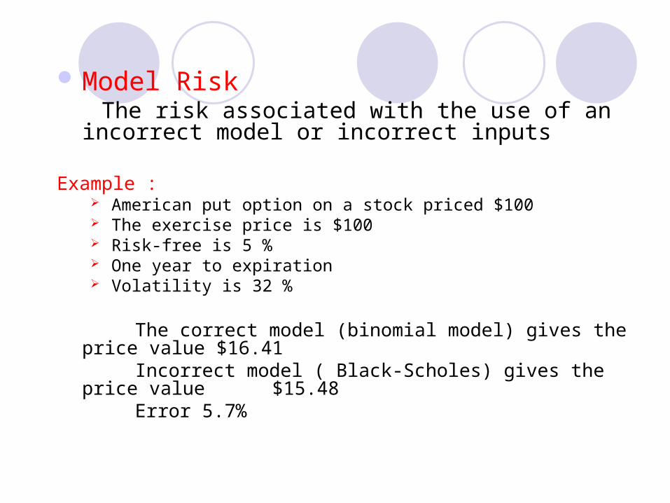
Model Risk The risk associated with the use of an incorrect model
or incorrect inputs
Example : American put option on a stock priced $100 The exercise price is $100 Risk-free is 5 % One year to expiration Volatility is 32 %
The correct model (binomial model) gives the price value $16.41 Incorrect model ( Black-Scholes) gives the price value $15.48 Error 5.7%

Failure to meet Assumption Major Assumptions Lognormality Randomness
Known and constant volatility
Minor Assumptions Known and constant risk-free rate No taxes and transaction costs American-style option

Major Assumptions
Lognormality The rate of return on the underlying asset is lognormally distribution.
Example: A non-dividend –paying stock sells for $100 and moves up to $110 after one
year. The logarithmic return is ln(1.10) = 9.53% The model typically assume the logarithmic return follows a normal
distribution, which means the return itself follows a lognormality distribution
Randomness Prices are randomness to assure that markets are competitiveness that allows
pricing models to work. No one participant can dominate all the others.
Known and constant volatility The volatility in standard option-pricing models is not directly observe and easy
to obtain. Also, the models are sensitive to the volatility.

Minor Assumptions1. Known and constant risk-free rate
Option-pricing models generally assume a known and constant risk-free rate.
2. No taxes and transaction costs
It facilitates the capture of most essential elements of the economic process being modeled.
3. American-style option
The option is the one that can be exercised before
expiration. It offers more flexibility.

Difficulty of Estimating Inputs 1. Market Value of the Underlying Asset Sometimes, the estimating for appropriate discount rate, the life of a
project may be difficult. 2. Exercise Price The amount of money can be received or paid in the future are difficult
to determine.
3. Time to Expiration A company can’t know how long it can keep a project before
abandoning it to claim a salvage value.
4. Volatility The option prices are very sensitive to the estimate of volatility. But it is
very difficult to observe in financial option-pricing application.

5. Risk-Free Rate The value of an option is not so sensitive to estimate of the risk-free
rate.
It is acceptable to obtain an estimate of the risk-free rate by estimating the rate on a default-free zero-coupon security.
Example
A real option expires in 275 days
Let the bid and ask discount rates on US government zero-coupon bonds (Treasury Bills) for maturity be 4.52% and 4.54%
We spilt the difference and assume a rate of 4.53%
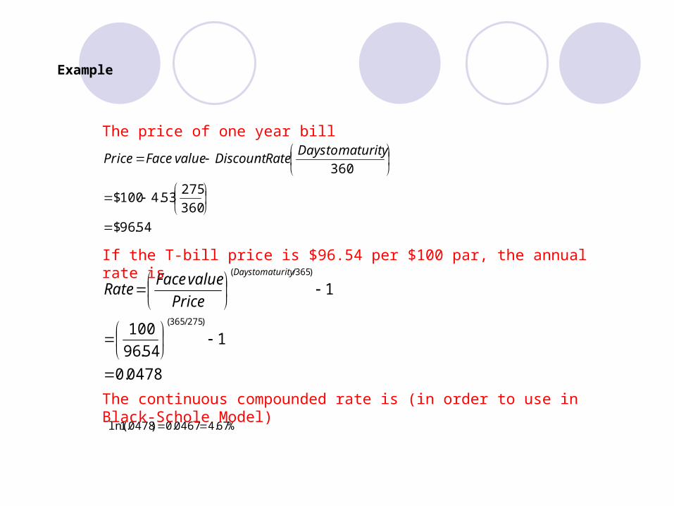
Example
54.96$
360
27553.4100$
360
maturitytoDaysRateDiscountvalueFaceicePr
0478.0
154.96
100
1
)275/365(
)365/(
maturitytoDays
Price
valueFaceRate
%67.40467.0)0478.1ln(
If the T-bill price is $96.54 per $100 par, the annual rate is
The continuous compounded rate is (in order to use in Black-Schole Model)
The price of one year bill
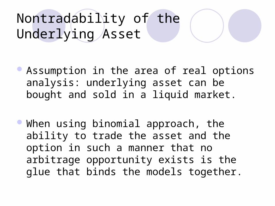
Nontradability of the Underlying Asset
Assumption in the area of real options analysis: underlying asset can be bought and sold in a liquid market.
When using binomial approach, the ability to trade the asset and the option in such a manner that no arbitrage opportunity exists is the glue that binds the models together.

Assumptions of Hedging, Tradability, and Risk Neutral Valuation
r: Risk-free rate (5%) u: Holding period return on the stock if it goes
up ($150) d: Holding period return on the stock if it goes
down ($50) Stock price: $100
55.05.05.1
50.005.11
du
drp

Option price calculation
19.26$05.1
)0($45.0)50($55.0
c

Risk-adjusted discount rate and probability of outcomes
If the probability of up move is 0.6, then Risk-adjusted discount rate k = 0.1.
If k = 0.12, then q=0.62.
k
1
)50)($1()150($100$

Risk-adjusted discount rate and probability of outcomes (cont.) If k is risk-free rate, then
q plays the same role as p in the option-valuation problem. Option-pricing models are often said to use risk neutral valuation.
pq
q
55.005.1
)50)($1()150($100$

Consistency of All Approaches
No one assume investors are risk neutral. Rather, risk neutral valuation is simple and imposes only light demands.
Risk neutral valuation is not a different approach that obtains different numbers from a standard risk-adjusted approach.(Feinstein 1999)

Example
Invest $9 in a project If the outcome is good, invest $18 and begin to
generate $10 a year forever. If the outcome is bad, invest $18 and begin to
generate $3 a year forever. Probability of good outcome is 0.6 and bad
outcome is 0.4 Discount rate is 25%

Example (cont.)
The market value of the project is:
The market value of the project at time 1 is:
12$25.0
3$
or 40$25.0
10$
1
1
B
G
V
V
6$18$12$
or 22$18$40$
1
1
B
G
X
X

Example (cont.) The value of the project at time 0 is:
NPV is
Up factor:
Down factor:
The risk neutral probability is
64.8$25.1
)]6.0$(4.0)22($6.0[0
V
5463.264.8
22$u
6944.064.8$
6$
d
5383.0)6944.0(5463.2(
)6944.0(05.1
p
36.0$9$64.8$

Example (cont.)
Option value $11.28
According to Feinstein’s approach, the overall discount rate is a blend of 25% and 5%. So the weighted discounted rate is:
The correct project value is
$11.28
05.1
)0($4617.0)22($5383.0
0.1704
1)0($4617.0)22($5383.0
)05.1)](0($4.0)22($6.0[
1- )1(
)1]()1([
11
11
BG
BG
w XppX
rXqqXk
1704.01
)0($4.0)22($6.0

Summary
One source of difficulty in applying real options valuation is the assumption may or may not be appropriate in the case of real options (lognormality distribution of the value of the underlying asset, randomness of prices)
The estimation of inputs, such as the volatility of the value of the underlying asset, the exercise price, the time to expiration, is more challenging for real options than for fincial options.

Chapter 6: Empirical Evidence on the Use and Accuracy of
Real Options Valuation

Paddock, Siegel, and Smith (1988) – Option Valuation of Claims on Real Assets: The Case of Offshore Petroleum Leases
Real options model for valuing offshore oil and gas leases in a federal sale of 21 tracts in the Gulf of Mexico.
Real options were not able to explain the bids as well as one might have hoped. Real options theory was not very well-known in 1988. Data provided by the government were not too good
to carry out analysis. Winner’s curse – tendency for the highest bidder to
pay more than fair

Quigg (1993) – Empirical Testing of Real Option-Pricing Models
Market prices of 2,700 land transactions in Seattle during 1976-1979. Market prices reflect a premium for the option to wait
to invest (optimal development) that has a mean value of 6% of the land value.
Supports the belief that investors either use real options models or trade in such a manner that their valuations are consistent with those of real options models.

Berger, Ofek, and Swary (1996) – Investor
Valuation of the Abandonment Option Whether investors price the option to abandon a firm
at its exit value.
This option is priced as an American put, whose value increases with exit value. Significant relationship between a company’s market
value and its estimated exit value, suggesting that investors take the option to exit into account when valuing companies.
The more likely the option will be exercised, the more valuable is the option.

Hayn (1995) – The Information Content of Losses
Hypothesizes that because shareholders have a liquidation option, losses are not expected to perpetuate. They are thus less informative than profits about the firm’s future prospects. The results are consistent with the hypothesis. Investors do not respond to losses to the same
magnitude that they do to profits. Option to liquidate is valued by investors.

Moel and Tufano (2002) – When Are Real Options
Exercised? An Empirical Study of Mine Closings
The flexibility that mining firms have to open and close mines. The overall pattern of closures is well predicted by real
option theory. Closures are influenced by the price and volatility of gold,
firm’s operating costs, proxies for closing costs, and the size of reserves.
Fail to capture aspects of firm-level decision making. Divisions within a firm share a common destiny and
decision about particular units are influenced by the performance of the other parts of the firm.

Clayton and Yermack (1999) – Major League Baseball Player Contracts: An Investigation of the Empirical Properties of Real Options
Contracts negotiated between professional baseball players and teams to investigate the use of real options in a commercial setting.
Baseball contracts feature options in diverse forms, and they found that these options have significant effects on player compensation. As predicted by theory, players receive higher guaranteed
compensation when they allow teams to take options on their future services, and lower salaries when they bargain for options to extend their own contracts.
The apparent value of options decreases as a function of the "spread" between option exercise price and annual salary and increases as a function of the time until exercise.

Howell and Jagle (1997) – Laboratory Evidence on How Managers Intuitively Value Real Growth Options
Asked managers series of questions on growth options from some investment case studies, asked other questions related to their personal situations and the kinds of investment decisions they make in their work. Skilled managerial decision makers agree only approximately with
real option theory. They tend on average to value growth options in an erratic way. Overvaluation seems to be a function of “Industry”, being lowest in
the oil industry, and it is also a function of (Business) “Experience” and “Position” being highest for more senior people.
The result can be interpreted in two ways: This limited sample of managers is not sufficiently knowledgeable
about real options models. Real options models are simply not used in practice. Small sample size is a major limitation of this study (82 managers)

Busby and Pitts (1997) - Real options in practice: an exploratory survey of how finance officers deal with flexibility in capital appraisal
Dissatisfaction with discounted cash flow techniques has lead to a growing literature focusing on the value of managerial flexibility in handling real asset investments, a subject area known as real options.
An exploratory survey of senior finance officers in industrial firms, examining the significance that real options assumed in their investment decisions, whether their firms had established procedures for assessing real options, and whether their intuitions were consistent with what theory prescribes.
There was wide variation between individual decision-makers in their perception of real options.
Few firms have procedures to assess options in advance. Very few decision-makers seemed to be aware of real option research but,
mostly, their intuitions agreed with the qualitative prescriptions of such work.

Chapter 7: Summary and Conclusions

Companies are often highly misvalued in the market Corporate investment decisions are typically made
using standard discounted cash flow (DCF) techniques, which are not equipped to accommodate real options
Discounted cash flow techniques that attempt to capture flexibility are not adequate
The valuation of financial options has benefited from years of study, evolving from the binomial and Black–Scholes models.
A number of limitations and difficulties arise in applying real options

Real options models oftentimes do not meet the assumptions inherent in the models
The estimation of inputs in real options models is particularly challenging
The models are based on the idea that one can trade the underlying asset and the option to form a risk-free hedge or trade a combination of the underlying asset and risk free bonds to replicate the payoffs of the option
Empirical research has provided some, but very limited, support for the real-world applicability of real options models

Thank youThank you


