Real-time Adaptive Non-holonomic Motion Planning in UnforeseenDynamic Environments

Sterling McLeodDepartment of Computer Science

University of North Carolina at CharlotteEmail: smcleo12@uncc.edu

Jing XiaoDepartment of Computer Science

University of North Carolina at CharlotteEmail: xiao@uncc.edu

Abstract— This paper addresses the problem of real-time,non-holonomic motion planning in environments with movingobstacles of unforeseen, arbitrary motion. An approach is in-troduced to smoothly switch trajectories by generating feasiblenon-holonomic trajectory segments on the fly as the robotmoves in such an environment, extending the real-time adaptivemotion planning (RAMP) approach that is used for holonomicmotion. It allows efficient on-line simultaneous planning andexecution of non-holonomic trajectories and enables a robot toadapt to changes in the environment while taking into accountrobot motion uncertainty. The effectiveness and efficiency ofthe method has been verified through real experiments witha mobile robot and several dynamic obstacles of unforeseenmotion to the robot.

I. INTRODUCTION

Non-holonomic motion planning is necessary for au-tonomous navigation of many real-world mobile robots. Thetopic has inspired nearly three decades of study [1]-[12].Early research was focused on the constraints and kinematicmodel of non-holonomic motion and algorithms to generatesteering inputs or non-holonomic paths [1]-[6]. These earlyalgorithms do not consider obstacles in an environment orhow to plan non-holonomic trajectories in real-time.

The popular sampling-based method of rapidly exploringrandom trees (RRT) [7] samples a robot’s configurationspace and grows a tree structure to produce a path thatis collision-free and satisfies kinematic constraints, such asnon-holonomic constraints. However, it is not inherentlyadaptive to changes in an environment. Genetic algorithm ap-proaches to non-holonomic motion planning have also beenexplored [9]-[11]. The planner in [9] uses a control-basedstrategy to ensure non-holonomic constraints are satisfied ona path, but does not consider real-time planning or obstacles.Generating non-holonomic trajectories in real time was pre-sented in [8] by using parametric representations to convertthe control problem into a nonlinear programming problem.This work, however, does not consider unpredictable movingobstacles in an environment.

Bezier curves for motion planning have been studiedfor several years, [13]-[16]. Bezier curves can be foundanalytically by specifying control points, which makes themuseful for on-line planning. They also allow smoother tra-jectories with higher speed than Reeds and Shepp curves

[17]. The work done by Choi et al., [13] and [14], focuseson connecting several curves to create a non-holonomic path.This requires using higher order curves that can be too costlyto generate in real-time. In [15], on-line conversion of agiven holonomic path to a non-holonomic and collision-free one using Bezier curves was presented. Similar workwas done in [16] by generating B-spline curves on-line foroptimized motion in aerial robots, which assumed that pathswere provided by a higher-level planner, without consideringmoving obstacles of unpredictable motion.

Most of the existing study of autonomous navigation of anon-holonomic robot is in the context of intelligent vehicles[18]-[20], where the environments are well-defined roads,and the robot (or self-driving vehicle) moves among othervehicles moving in the same general direction. However,there is little research on autonomous non-holonomic navi-gation among obstacles that can move in arbitrary directionsand can either move or stop indefinitely in an environment.Such an environment is possible, for example, in a warehousesetting with mobile robots transporting goods, where everyrobot has to avoid collision with moving obstacles, such asother robots, other vehicles, or people, without knowing theirmotion beforehand.

The concept of velocity obstacles and its variants [21]-[23]have been used to prevent a robot colliding with anotherrobot. However, it does not apply to cases with arbitraryobstacles of unforeseen motion.

Real-time obstacle avoidance using potential fields hasbeen studied extensively [24]-[26]. Much of the work treatslocal navigation as a control problem and does not considerthe global objective of reaching a goal. The Elastic Roadmapmethod [27] achieves local navigation and global objectiveplanning by using potential fields for navigation and usingsampling to build a global roadmap. However, the robot’smobile base motion is holomonic, and the environmentshown is mostly static. Inevitable collision states are alsoan important factor in obstacle avoidance [28].

The real-time adaptive motion planning (RAMP) frame-work [29] enables simultaneous planning and executionof robot motion in a dynamically unforeseen environment.It provides seamless integration of explicit global motionplanning under optimization criteria and local navigation to

enable a robot to reach its goal with real-time adaptiveness.However, this work focuses on a mobile manipulator withan omnidirectional base rather than a non-holonomic base.

In this paper, we address the problem of real-time motionplanning to allow non-holonomic robot motion in envi-ronments with dynamic obstacles of unforeseen, arbitrarymotion. We introduce an approach to smoothly switch tra-jectories by generating non-holonomic trajectory segmentson the fly as the robot moves in such an environment, ex-tending the RAMP approach for non-holonomic motion. Ourapproach combines Bezier curves and straight-line segmentsto produce non-holonomic and smooth trajectories in realtime. It is characterized by the following features:• Global search and real-time adaptation of hybrid tra-

jectoriesLike the RAMP approach, our planner allows for real-time, simultaneous global path and trajectory planningand execution of trajectories. However, the trajectoriesthat our planner creates begin with non-holonomicsegments of Bezier curves followed by straight-line(holonomic) segments. Planning such hybrid trajectoriesallows for high efficiency for on-line operation; only theimmediate trajectory segment that a robot moves alongis converted to satisfy non-holonomic constraints.

• Smooth switching of trajectoriesOne trademark of RAMP’s real-time adaptiveness isallowing the robot to switch to better trajectories onthe fly to adapt to changes in a dynamic environment.However, switching of non-holonomic trajectories ismore challenging due to the kinematic constraints. Ourplanner enables smooth switching and utilizes the Re-flexxes trajectory library [30] to produce trajectories thatsatisfy switching conditions almost instantly.

• Adaptation of planned trajectories to motion errorReal-world execution of a trajectory is inevitably af-fected by robot motion error. Our planner uses predic-tions of the robot’s future states to plan trajectories.However, motion error can make a prediction incorrectbecause the actual state that the robot reaches can bedifferent. Our planner uses sensing feedback to adjustpredictions to minimize the effect of motion error.

Note that this work emphasizes adaptability rather thanoptimality. It is not possible to achieve global optimalityof robot motion in environments with unforeseen obstaclemotions. Our algorithm maintains and evolves a number oftrajectories in order to give a robot options for adaptation tochanges in an environment. If all future obstacle motion wereknown, the algorithm could be set to maintain and improve asufficiently large and diverse population to achieve globallynear-optimal results.

In contrast to a known or static environment, in a dynamicenvironment with unforeseen changes, on-line simultaneouspath/trajectory generation and execution is necessary for arobot to adapt to changes while achieving its goal.

The rest of the paper is organized as follows: SectionII describes our method of generating hybrid trajectories.Section III details the different aspects of the planner for

generating smooth transitions, adaptive control cycles, trajec-tory evaluation, and population improvement. Next, SectionIV discusses implementation and real experimental results.Section V concludes the paper.

II. GENERATION OF NON-HOLONOMIC TRAJECTORYSEGMENTS

A mobile robot can be either holonomic or non-holonomic.Its configuration can be expressed as (x, y, θ). Its state canbe expressed as a point (x, y, θ, t) in its configuration-time(CT) space. A trajectory is represented as a set of states inthe robot’s CT space. A non-holonomic trajectory satisfiesthe non-holonomic constraint:

−x sin θ + y cos θ = 0 (1)

which is necessary for a non-holonomic robot and is desir-able for a holonomic robot (if it is not omnidirectional) toconduct smooth motion. A non-holonomic segment is any setof continuous points on a trajectory that satisfy equation (1).Such a segment may consist of curves and straight lines, aslong as all points satisfy the non-holonomic constraint. Anysegments that require the robot to stop and rotate in placeare not non-holonomic segments.

Given a holonomic path consisting of straight-line seg-ments (generated by the RAMP-H planner, detailed in Sec-tion III), the algorithm converts the first two straight-linesegments to a non-holonomic segment by creating a Beziercurve to connect the two straight-line segments, as shownin Fig. 1a. Velocity and acceleration values that satisfy therobot’s motion constraints are generated for each point onthe curve, as detailed below.

(a) Example hybridtrajectory

(b) Robot has incor-rect orientation

(c) Bezier curveadded to enablemoving on trajectory

Fig. 1: Hybrid trajectory examples

Each Bezier curve for connecting two straight-line seg-ments is defined by three control points (X0, Y0), (X1, Y1),and (X2, Y2), as shown in Fig. 2, and can be expressed interms of a parameter u [15]:

x = (1− u)2X0 + 2u(1− u)X1 + u2X2

y = (1− u)2Y0 + 2u(1− u)Y1 + u2Y2

(2)

The velocity and acceleration along the curve can be furtherderived as functions of u and u:

x = (Au+ C)u

y = (Bu+D)u(3)

x = (Au+ C)u+Au2

y = (Bu+D)u+Bu2(4)

where A = 2(X0 − 2X1 + X2), B = 2(Y0 − 2Y1 + Y2),C = 2(X1 −X0), and D = 2(Y1 − Y0). (X0, Y0) is chosenon the first straight-line segment. (X1, Y1) is the knot pointconnecting the two straight-line segment, and (X2, Y2) ischosen on the second straight-line segment, such that A, B,C, and D are not zero.

Fig. 2: A quadratic Bezier curve connecting two straight linesegments

The Reflexxes Type II library [30] is used to generatesmooth motion for a hybrid path. For each straight-linesegment, we apply Reflexxes to generate the trajectory for xand then compute the corresponding trajectory for y as thelinear function of x. For the Bezier curve, Reflexxes is usedto generate u, u, and u values for a trajectory of u and thosevalues are substituted into the above equations to obtain thecorresponding non-holonomic trajectory.

There are two u values that are necessary to specifyto generate a trajectory using Reflexxes - the initial andmaximum u. The initial u can be found when u is zero:

u0 =x0C

=y0D

(5)

where x0 and y0 are the velocities at the start of the curve(i.e., at the curve’s first control point).

The maximum velocity umax can be decided by settingu = 0. If a maximum of u exists, it can be obtained by:

umax = min(

√xmaxA

,

√ymaxB

) (6)

where xmax and ymax are determined by the robot’s velocitylimits. Otherwise, the value of u0 is used for umax.

Note that if a Bezier curve makes too sharp of a turn, i.e.,one with large curvature values, the robot may not be able tofollow it. The maximum angular velocity on a curve occursat the point ur, which is the point of minimum radius Rminalong the curve, as derived in [15]:

ur = −AC +BD

A2 +B2(7)

Rmin =

√[(A2 +B2)u2r + 2(AC +BD)ur + (C2 +D2)]3

(BC −AD)2.

(8)

For a given Bezier curve, we can use the values of urand umax and equation (3) to make a conservative (i.e.,worst-case) estimation of the robot’s linear and angularvelocities, vr and ωr respectively, required at ur. If therobot’s maximum angular velocity is not large enough, i.e.ωmax < ωr, then the robot cannot follow the Bezier curve.

If a robot’s starting orientation is not aligned with thebeginning straight-line portion of the non-holonomic tra-jectory segment (converted from the first two straight-linesegments of a holonomic path, as described above), asshown in Fig. 1b, the robot cannot readily execute thenon-holonomic trajectory segment. That often happens whentrajectory switching is needed. In such a case, a straight-linesegment aligned with the robot’s starting orientation and aBezier curve are added to form a non-holonomic transitiontrajectory, as shown in Fig. 1c, to enable the robot smoothlyget on the original non-holonomic segment.

The result is a hybrid trajectory, consisting of up to twoBezier curves followed by straight-line holonomic segments,allowing smooth transition of the robot from one straight-linesegment to the next.

III. ONLINE PLANNING AND EXECUTION: RAMP-H

We extend the RAMP approach to plan hybridpaths/trajectories that combine non-holonomic and holo-nomic segments. The approach progressively converts holo-nomic segments to non-holonomic segments on the fly forexecution by the robot. This real-time hybrid planner, calledRAMP-H, enables smooth and adaptive non-holonomic mo-tion of the robot towards its goal while avoiding dynamicobstacles of unforeseen motion in the environment.

A. Overview

RAMP-H conducts planning and execution of motionsimultaneously via planning, control, and sensing cycles.Planning cycles modify a set of trajectories, called a popu-lation, to find a better trajectory for the robot to move on.Unlike the other cycles, planning cycles are not set to occurat specified intervals. When one planning cycle finishes, anew one begins immediately. At each control cycle, the robotwill switch to the best trajectory in the population. As therobot moves, changes in the environment are captured andupdated in each sensing cycle and conveyed to the plannerto facilitate adaptation.

Algorithm 1 outlines our method. Our planner starts fromgenerating an initial population of holonomic trajectories thatall start from the same initial state of the robot, and each tra-jectory consists of straight-line segments and self-rotations,where the knot configurations connecting the straight-linesegments can be generated randomly. The procedure convertis then called to add a non-holonomic segment at thebeginning of each trajectory to enable a smooth transition ofthe robot to the first straight-line segment of that trajectoryand also convert the first two straight-line segments of thetrajectory into a non-holonomic segment (as described inSection II). The result is a population of hybrid trajectoriesstarting from two non-holonomic segments followed byholonomic segments. Section III-B provides more details ofconvert. Next, The procedure evaluate is called to evaluateand rank the fitness of the hybrid trajectories, as detailed inSection III.C. The best trajectory is obtained for the robot tomove on.

Algorithm 1 RAMP-H overview

1: Set control and sensing cycle time ∆tc and ∆ts respec-tively;

2: i← 1; //index of control cycle3: initialize a population P1 of holonomic trajectories;4: convert P1 to hybrid trajectories PH1 ;5: evaluate PH1 and obtain the best trajectory τ16: and the portion τ1,c within the first ∆tc of τ1;7: t1 ← 0; //beginning time of 1st control cycle8: t2 ← ∆tc; //beginning time of 2nd control cycle9: τbest ← τ1;

10: while goal is not reached do11: simultaneously do Move, Plan, and Sense:12: Move:13: if τi,c is feasible or collision on τi,c is not expected14: within time period tthresh then15: move along τbest;16: else17: pause motion;18: Plan:19: if beginning of ith control cycle then20: ti+1 ← ti + ∆tc;21: obtain Pi+1 by updating the starting state of Pi;22: convert Pi+1 to PHi+1 and find the earliest23: starting time ti+1,e in Phi+1;24: ti+1 ← ti+1,e

25: adjust Pi+1 and PHi+1;26: evaluate PHi+1;27: modify Pi+1;28: if end of ith control cycle then //reaching time ti+1

29: i← i+ 1;30: τbest ← τi //update best trajectory31: Sense:32: if new sensing cycle then33: evaluate PHi+1;34: collision-check τi,c;

During the first control cycle, the robot moves along thebest trajectory, τ1, as long as its portion within the firstcontrol cycle, τ1,c, is collision-free. Note that the durationof a control cycle ∆tc is set to ensure that τ1,c is non-holonomic. While the robot moves along τ1,c, the planneris simultaneously improving the population of trajectoriesso that at the next control cycle, the robot can switch toa better trajectory if available. For that purpose, at thebeginning of the current control cycle, the planner updatesthe starting states of all other trajectories (except for thecurrently being executed one) to be the state at the beginningof the next control cycle and converts the updated trajectoriesto be hybrid ones. Note that the conversion can changethe starting time of the next control cycle because differenthybrid trajectories require different starting times (SectionIII-B).

The planner improves the trajectories by calling adjust,evaluate, and modify repeatedly in multiple planning cycles

(i.e., the while loop), detailed in Section III-C. During robotmotion and planning, sensory updates of the environmentare conducted every sensing cycle, and the trajectories arere-evaluated and re-ranked to reflect the changes in theenvironment. Re-evaluating is necessary because the previousbest trajectory may no longer be the best after changes occurin the environment. If the best non-holonomic trajectorysegment τi,c is not collision-free and the collision is expectedto occur within time period, tthresh, then the robot’s motionwill be paused to wait for the planner to find a collision-freetrajectory through more planning cycles. The value of tthreshis chosen such that the robot stops early enough to allow fora non-holonomic motion around a stopped obstacle. If theobstacle moves away from τi,c before ti+1, then the robotwill resume its motion along τbest.

In the following subsections, procedures convert, evalu-ate, adjust, and modify are explained in detail.

B. Smooth Trajectory Transition and Adaptive Control Cy-cles

Given a population P of holonomic trajectories, whereeach is in terms of knot configurations connecting straight-line segments, the procedure convert obtains a popula-tion of hybrid trajectories PH from P by adding a non-holonomic transition trajectory segment, if necessary, fol-lowed by converting the first two straight-line segments toa non-holonomic trajectory segment, as described in SectionII, for each trajectory in P . At each control cycle, after thestarting states of trajectories are updated to be the states at thenext control cycle, convert is called on the new populationto prepare non-holonomic segments.

Note that a transition trajectory segment has to occurbefore the next control cycle in order for the robot tosmoothly switch to the intended trajectory by the time ofthe next control cycle. Thus, a transition trajectory consistsof a Bezier curve to connect the straight-line segment of thecurrent trajectory before transition and the first straight-linesegment of the new trajectory. The segment points (X0, Y0),(X1, Y1), and (X2, Y2) for a transition curve are the robot’scurrent position, the future position at the next control cycle,and the first control point of the target trajectory’s Beziercurve, respectively.

The control points of the transition curve for a trajectory,however, depend on the robot’s kinematic constraints and thesharpness of the curve needed for transition. We divide thecontrol cycle period ∆tc into m steps. Starting at the timeof the mth step, our system assigns the (future) position ofthe robot at that time as the first control point and attemptsto plan a kinematically feasible transition trajectory. If sucha trajectory cannot be found, the position at the m-1th step isused. Our system continues this process until either it findsa kinematically feasible transition trajectory or the possiblepositions at all steps are exhausted so that no switching willbe possible to that trajectory. Different trajectories are likelyto have different first control points.

Fig. 3 shows an example. In Figure 3(a), the robot is mov-ing on the best trajectory, T , at the current time and wants

(a) Robot wants toswitch from T to T ′

(b) Transition trajec-tory shown in blue

(c) Full switchshown in blue

Fig. 3: Switching trajectories

to compute a transition trajectory to switch to trajectory T ′.The next control cycle is expected to occur in ∆tc secondsand is at point pcc. The trajectories’ curves between their firsttwo segments are labelled as C and C ′. The motion statesat pc and p′c are the initial states of their respective curves.

The transition trajectory can be seen in 3(b) as the solidblue line. It consists of a Bezier curve, Cs, that begins at oneof the future time steps and a straight-line segment that endsat the first control point of C ′. Once the transition trajectory,Ttrans, has been created, the curve from the target trajectory,C ′, and the remaining points on T ′ are concatenated ontoTtrans to form Tnew. In Figure 3(c), Tnew is shown in blue.

It is unlikely that all trajectories in the transition popu-lation will begin at the same time. Therefore, the startingtime of the next control cycle is set to be the earliest startingtime among all transition trajectories in Algorithm 1, i.e., thefrequency of control cycles is determined both by the needof non-holonomic conversion of trajectories for the robotto follow and the need for the robot to switch to a bettertrajectory. Thus, the interval of an actual control cycle isadaptive, unlike in the previous RAMP design [29].

C. Trajectory Evaluation

Procedure evaluate calls an evaluation function to measurethe fitness of each hybrid trajectory so that trajectories canbe ranked based on their fitness. The evaluation functionconsiders the total time it takes to execute a trajectory, T ,and the change in orientation required to move along thattrajectory, ∆θ. The initial orientation when calculating ∆θis the robot’s current orientation and the ending orientation isthe angle required to move on the trajectory’s first segment.

1) Feasible trajectories: The cost for a feasible trajectory,which is defined as a trajectory with no collision in its non-holonomic portion, is the sum of the weighted, normalizedvalues for T and ∆θ.

Costfe = C1T

a1+ C2

∆θ

a2(9)

where Ci is a weight, and ai is a normalization value.2) Infeasible trajectories: Infeasible trajectories are de-

fined as those with collision in the non-holonomic portion.The cost equation is a sum of two penalties:

Costin = PT + Pθ (10)

PT =QTTcoll

and Pθ = Qθ∆θ

M(11)

where QT and Qθ are large constant values, Tcoll is the timeof the first collision in the trajectory, ∆θ is the orientationchange from Eq. (9), and M is a normalization term.

The penalty PT ensures that trajectories with collisionsexpected earlier will be penalized more than trajectories withcollision expected later. Pθ ensures that trajectories withlarger orientation change are penalized more. QT and Qθare set such that the penalty for a large orientation changewill not be larger than for collision. No infeasible trajectorywill ever be fitter than a feasible one.

Procedure evaluate only checks for collision in the non-holonomic segments of a trajectory to take into accountthe fact that the environment may change in unpredictableways, trajectories are constantly evolved, and thus non-holonomic conversion occurs later for later segments andwill be checked for collision then. This saves a lot of time.Collision checking is conducted between the robot’s non-holonomic trajectory segment and the predicted trajectorysegment for the same time period of every obstacle.

3) Obstacle trajectory prediction: Obstacle trajectoriesare predicted based on the last known motion state of anobstacle. The last known linear and angular velocity values,v(ti) and ω(ti), respectively, are used to determine one ofthree simple types of motion for an obstacle during thecurrent sensing cycle: translation only with non-zero v(ti)and zero ω(ti), self-rotation if v(ti) is zero and ω(ti) non-zero, or global rotation if both v(ti) and ω(ti) are non-zero.If an obstacle’s velocity changes after a sensing cycle, thenew motion will be updated at the next sensing cycle. Thefrequency of sensing cycles is high enough to update theobstacle motion quickly enough for real-time avoidance.

4) Further discussion: As shown in Algorithm 1, theRAMP-H planner calls evaluate in each cycle: each planningcycle calls evaluate to get the fitness for new trajectories,each sensing cycle calls evaluate to update the fitness of eachtrajectory to take the environment changes into account, andeach control cycle calls evaluate after the starting state ofthe trajectory population is updated and the non-holonomicsegments are subsequently updated. Only the updated (be-ginning) non-holonomic segment of each trajectory is re-evaluated to reduce the computational cost; the evaluationresults of the remaining holonomic segments are re-used.

Even though each hybrid trajectory does not representthe exact motion that the robot will execute (because futureholonomic segments can be changed and will be converted),the evaluation results are still representative of relative fitnesswithin the population because the holonomic segments takeinto account the cost of translation and rotation. Hence, thehybrid trajectory with the lowest cost represents the best non-holonomic trajectory in the population.

D. Improvement of Trajectories Based on Sensing

The RAMP-H planner improves hybrid trajectoriesthrough the following operations.

1) Adjust: At each control cycle, the new population Pi+1

is obtained by updating the starting state of Pi. The updatedstate is the robot’s intended future state at the next controlcycle based on its current trajectory. However, this updateassumes perfect motion of the robot. Due to motion error, therobot may not reach this state and may encounter unpredictedcollision as a consequence. The adjust procedure is calledin each planning cycle (i.e., the while loop in Algoritm 1)to address this issue.

The procedure adjust polls the robot’s internal sensors toobtain the robot’s current motion state. The difference be-tween the robot’s current position and the expected positionalong the current trajectory at the time of the planning cycleis added to the position of the state scc at the beginningof the next control cycle as an offset. The positions inall the trajectories of the population starting at scc areoffset accordingly. Although the act of offsetting is quitesimple, the significance of this method is that it relies on theinteraction of planning and control cycles to treat specifictime cycles as clear, unambiguous landmarks in time toperform the adjustment.

If the robot is stopped indefinitely by imminent collision,then the adjust procedure allows the planner to plan alterna-tive trajectories for the robot from where the robot is stopped.

2) Modify: In each planning cycle, the planner also callsthe procedure modify to hopefully improve the population oftrajectories. In procedure modify, a subset of trajectories arerandomly selected, and next the knot configurations (i.e., theholonomic paths) are altered by common genetic operatorsas used in the RAMP planner [29]: Insert, Delete, orChange a knot configuration, Swap the order of two knotconfigurations, and Crossover two trajectories. New trajec-tories are converted again into hybrid ones (if necessary)and evaluated. They are then used to replace some randomlyselected trajectories except for the best trajectory in theprevious population. However, an infeasible trajectory willnot replace a feasible one and a trajectory will not be added ifits fitness is less than the minimum fitness in the population.This approach mixes elitism and diversity in evolving atrajectory population over generations (i.e., planning cycles).

Note that our planner continuously improves trajectoriesthrough planning cycles while interacting with sensing cyclesto adapt trajectories to changes in the environment. Theplanner also interacts with control cycles to allow the robotto switch to trajectories best adapt to the environment. There-fore, the actual motion that the robot executes is most likelya concatenation of non-holonomic segments from differenthybrid trajectories along the way, as shown in Fig. 4.

IV. IMPLEMENTATION AND EXPERIMENTS

We have implemented our planner and tested it bothin real experiments and in simulation. Its effectiveness isverified by examples of experiments on real robots with

Fig. 4: Example motion from start to finish

several dynamic obstacles. The following subsections detailour implementation, experiment environments, and results.

A. Implementation and Experimental Setup

Our planner is implemented using C++ and utilizes theROS framework for message passing among the differentprocedures in Algorithm 1, and each procedure runs onits own ROS node. All processes other than the trajectoryfollowing and on-board control of the robot were run on anIntel i7 8-core CPU at 2.50GHz.

The robots used were two iRobot Creates, one KobukiYujin, and one CoroBot CL2 for testing, which are alldifferential-drive robots, and are commanded to conduct non-holonomic motion in our experiments.

In all experiments, one of the robots uses the RAMP-H planner, which we call the RAMP-H robot, and theother robots are employed as dynamic obstacles whosemotions are unforeseen by the RAMP-H robot. The obstaclerobots broadcast their sensed locations from odometry overa wireless LAN in order for the RAMP-H robot to predicttheir trajectories. The RAMP-H robot also uses its ownodometry to sense its own location to help adjusting itstrajectories. All of the robots except the Yujin use onlywheel encoders to sense their odometry. The Yujin utilizes aninternal gyroscope to better sense its orientation. No camerasor other external sensors are used to sense the obstacles. Thesensing frequency of each robot is 15Hz.

(a) (b)

(c) (d)

Fig. 5: The RAMP-H robot (circled in green) moving amongthree dynamic obstacles (circled in red)

The testing environment is a square of 3.5m × 3.5mon a carpet, flat floor. The RAMP-H robot starts from onecorner of the square and needs to reach its destination at thecorner across the diagonal while avoiding moving obstaclesof unforeseen motion. For both the RAMP-H robot and each

(a) (b)

(c) (d)

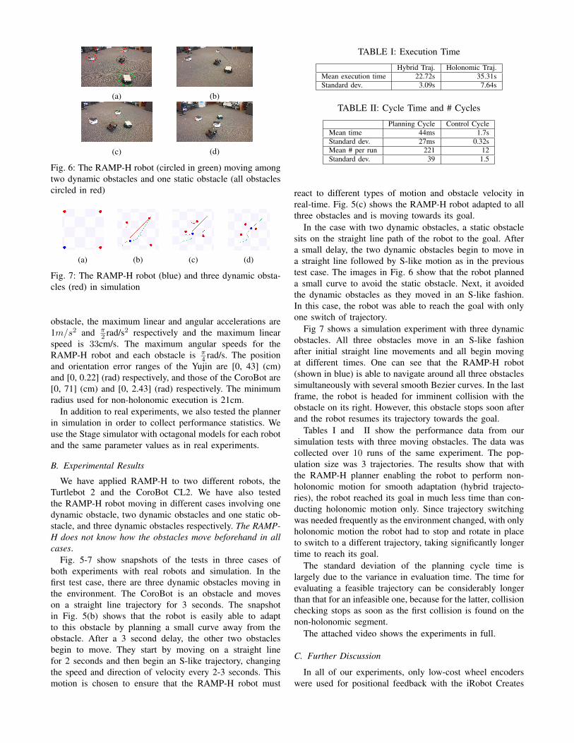
Fig. 6: The RAMP-H robot (circled in green) moving amongtwo dynamic obstacles and one static obstacle (all obstaclescircled in red)

(a) (b) (c) (d)

Fig. 7: The RAMP-H robot (blue) and three dynamic obsta-cles (red) in simulation

obstacle, the maximum linear and angular accelerations are1m/s2 and π

2 rad/s2 respectively and the maximum linearspeed is 33cm/s. The maximum angular speeds for theRAMP-H robot and each obstacle is π

4 rad/s. The positionand orientation error ranges of the Yujin are [0, 43] (cm)and [0, 0.22] (rad) respectively, and those of the CoroBot are[0, 71] (cm) and [0, 2.43] (rad) respectively. The minimumradius used for non-holonomic execution is 21cm.

In addition to real experiments, we also tested the plannerin simulation in order to collect performance statistics. Weuse the Stage simulator with octagonal models for each robotand the same parameter values as in real experiments.

B. Experimental Results

We have applied RAMP-H to two different robots, theTurtlebot 2 and the CoroBot CL2. We have also testedthe RAMP-H robot moving in different cases involving onedynamic obstacle, two dynamic obstacles and one static ob-stacle, and three dynamic obstacles respectively. The RAMP-H does not know how the obstacles move beforehand in allcases.

Fig. 5-7 show snapshots of the tests in three cases ofboth experiments with real robots and simulation. In thefirst test case, there are three dynamic obstacles moving inthe environment. The CoroBot is an obstacle and moveson a straight line trajectory for 3 seconds. The snapshotin Fig. 5(b) shows that the robot is easily able to adaptto this obstacle by planning a small curve away from theobstacle. After a 3 second delay, the other two obstaclesbegin to move. They start by moving on a straight linefor 2 seconds and then begin an S-like trajectory, changingthe speed and direction of velocity every 2-3 seconds. Thismotion is chosen to ensure that the RAMP-H robot must

TABLE I: Execution Time

Hybrid Traj. Holonomic Traj.Mean execution time 22.72s 35.31sStandard dev. 3.09s 7.64s

TABLE II: Cycle Time and # Cycles

Planning Cycle Control CycleMean time 44ms 1.7sStandard dev. 27ms 0.32sMean # per run 221 12Standard dev. 39 1.5

react to different types of motion and obstacle velocity inreal-time. Fig. 5(c) shows the RAMP-H robot adapted to allthree obstacles and is moving towards its goal.

In the case with two dynamic obstacles, a static obstaclesits on the straight line path of the robot to the goal. Aftera small delay, the two dynamic obstacles begin to move ina straight line followed by S-like motion as in the previoustest case. The images in Fig. 6 show that the robot planneda small curve to avoid the static obstacle. Next, it avoidedthe dynamic obstacles as they moved in an S-like fashion.In this case, the robot was able to reach the goal with onlyone switch of trajectory.

Fig 7 shows a simulation experiment with three dynamicobstacles. All three obstacles move in an S-like fashionafter initial straight line movements and all begin movingat different times. One can see that the RAMP-H robot(shown in blue) is able to navigate around all three obstaclessimultaneously with several smooth Bezier curves. In the lastframe, the robot is headed for imminent collision with theobstacle on its right. However, this obstacle stops soon afterand the robot resumes its trajectory towards the goal.

Tables I and II show the performance data from oursimulation tests with three moving obstacles. The data wascollected over 10 runs of the same experiment. The pop-ulation size was 3 trajectories. The results show that withthe RAMP-H planner enabling the robot to perform non-holonomic motion for smooth adaptation (hybrid trajecto-ries), the robot reached its goal in much less time than con-ducting holonomic motion only. Since trajectory switchingwas needed frequently as the environment changed, with onlyholonomic motion the robot had to stop and rotate in placeto switch to a different trajectory, taking significantly longertime to reach its goal.

The standard deviation of the planning cycle time islargely due to the variance in evaluation time. The time forevaluating a feasible trajectory can be considerably longerthan that for an infeasible one, because for the latter, collisionchecking stops as soon as the first collision is found on thenon-holonomic segment.

The attached video shows the experiments in full.

C. Further Discussion

In all of our experiments, only low-cost wheel encoderswere used for positional feedback with the iRobot Creates

and Corobot. If more accurate sensing were used for feed-back, the error would be smaller to adjust for, but it wouldstill exist. By addressing the issue of adapting to the motionerror, our method puts planning and control in sync. Thefact that our implementation uses only low-resolution wheelencoders shows that motion and planning can be reasonablyin sync even with infamously inaccurate odometry sensorsalone; such robustness is important when there is limitedmeans of sensing the robot’s environment, e.g. if a cameracannot be used due to a dimly lit environment. With moreaccurate and faster sensors, the RAMP-H can be moreeffective in dealing with faster moving obstacles.

As shown in our experiments, the RAMP-H algorithm isvery useful because trajectory switching is needed frequentlyas the environment changes. With smooth non-holonomicmotion, not only can the robot switch trajectories much moreefficiently, but it can also eliminate the danger of beinghit by a moving obstacle while rotating in place to switchtrajectories.

V. CONCLUSION

This paper addresses simultaneous planning and executionof non-holonomic robot trajectories in an environment withmoving obstacles of unforeseen and arbitrary motion. Thiswork extends the RAMP algorithm [29] to handling hybridtrajectories of non-holonomic and holonomic segments. Thepresented RAMP-H algorithm enables a robot to move alongand smoothly change to a new non-holonomic trajectory onthe fly while taking into account the actual error in robotmotion execution in the process. The RAMP-H planner canbe improved with a more efficient implementation and moreeffective sensing of the environment and robot’s own statewith better sensors and sensory data processing. Further test-ing will be conducted to study RAMP-H in more challengingand cluttered environments.

VI. ACKNOWLEDGEMENT

The first author would like to gratefully acknowledge thesupport of the GAANN Fellowship from the U.S. Depart-ment of Education and from NSF Grant IIP-1266162.

REFERENCES

[1] J.-P. Laumond. Feasible trajectories for mobile robots with kinematicand environment constraints. In Intelligent Autonomous Systems, AnInternational Conference, pages 346–354, Amsterdam, The Nether-lands, 1987. North-Holland Publishing Co.

[2] C. Fernandes, L. Gurvits, and Z.X. Li. A variational approach tooptimal nonholonomic motion planning. In Proceedings of 1991 IEEEInternational Conference on Robotics and Automation, (ICRA), pages680–685 vol.1, Apr 1991.

[3] J. Barraquand and J.-C. Latombe. Nonholonomic multibody mobilerobots: Controllability and motion planning in the presence of obsta-cles. Algorithmica, 10(2-4):121–155, 1993.

[4] R.M. Murray and S.S. Sastry. Nonholonomic motion planning:steering using sinusoids. IEEE Transactions on Automatic Control,38(5):700–716, May 1993.

[5] J.-P. Laumond, P.E. Jacobs, M. Taix, and R.M. Murray. A motionplanner for nonholonomic mobile robots. IEEE Trans. Robot. Autom.,10(5):577–593, Oct 1994.

[6] B. Nagy and A. Kelly. Trajectory generation for car-like robots usingcubic curvature polynomials. Field and Service Robots, 11, 2001.

[7] S. Lavalle. Rapidly-exploring random trees: A new tool for pathplanning. Technical report, C.S. Dept., Iowa State Univ., 1998.

[8] A. Kelly and B. Nagy. Reactive nonholonomic trajectory generationvia parametric optimal control. The International Journal of RoboticsResearch (IJRR), 22(7-8):583–601, 2003.

[9] W. Cheng, Z. Tang, C. Zhao, L. Tang, and Z. Guo. Path planningfor nonholonomic car-like mobile robots using genetic algorithms. In2006 8th International Conference on Signal Processing, volume 4,2006.

[10] G. Erinc and S. Carpin. A genetic algorithm for nonholonomic motionplanning. In ICRA 2007, pages 1843–1849, April 2007.

[11] X.-S. Ge, H. Li, and Q.-Z. Zhang. Nonholonomic motion planning ofspace robotics based on the genetic algorithm with wavelet approxi-mation. In IEEE International Conference on Control and Automation,2007, pages 1977–1980, May 2007.

[12] D.G. Macharet, A.A. Neto, V.F. da Camara Neto, and M.F.M. Campos.Nonholonomic path planning optimization for dubins’ vehicles. InICRA 2011, pages 4208–4213, May 2011.

[13] J.-W. Choi, R. Curry, and G. Elkaim. Path planning based on beziercurve for autonomous ground vehicles. In Advances in Electricaland Electronics Engineering - IAENG Special Edition of the WorldCongress on Engineering and Computer Science 2008, WCECS ’08.,pages 158–166, Oct 2008.

[14] J.-W. Choi and K. Huhtala. Constrained path optimization with beziercurve primitives. In 2014 IEEE/RSJ International Conference onIntelligent Robots and Systems (IROS), pages 246–251, Sept 2014.

[15] Y. Li and J. Xiao. On-line planning of nonholonomic trajectories incrowded and geometrically unknown environments. In ICRA 2009,pages 3230–3236, May 2009.

[16] Dongwon Jung and Panagiotis Tsiotras. On-line path generation forsmall unmanned aerial vehicles using b-spline path templates. In AIAAGuidance, Navigation and Control Conference, AIAA, volume 7135,2008.

[17] J. Reeds and L. Shepp. Optimal paths for a car that goes both forwardsand backwards. Pacific journal of mathematics, 145(2):367–393, 1990.

[18] S. Thrun, M. Montemerlo, H. Dahlkamp, D. Stavens, A. Aron,J. Diebel, P. Fong, J. Gale, M. Halpenny, G. Hoffmann, et al. Stanley:The robot that won the darpa grand challenge. In The 2005 DARPAGrand Challenge, pages 1–43. Springer, 2007.

[19] D. Dolgov, S. Thrun, M. Montemerlo, and J. Diebel. Path planningfor autonomous vehicles in unknown semi-structured environments.IJRR, 29(5):485–501, 2010.

[20] M. Buehler, K. Iagnemma, and S. Singh. The DARPA UrbanChallenge: Autonomous vehicles in city traffic, volume 56. springer,2009.

[21] P. Fiorini and Z. Shiller. Motion planning in dynamic environmentsusing velocity obstacles. IJRR, 17(7):760–772, 1998.

[22] D. Wilkie, J. van den Berg, and D. Manocha. Generalized velocityobstacles. In IROS 2009, pages 5573–5578, Oct 2009.

[23] J. Snape, J. van den Berg, S.J. Guy, and D. Manocha. The hybridreciprocal velocity obstacle. IEEE Trans. Robot., 27(4):696–706, Aug2011.

[24] M. Khatib, H. Jaouni, R. Chatila, and J.P. Laumond. Dynamic pathmodification for car-like nonholonomic mobile robots. In ICRA 1997,volume 4, pages 2920–2925 vol.4, Apr 1997.

[25] O. Khatib. Real-time obstacle avoidance for manipulators and mobilerobots. IJRR, 5(1):90–98, 1986.

[26] D. Fox, W. Burgard, S. Thrun, et al. The dynamic window approachto collision avoidance. IEEE Robot. Autom. Mag., 4(1):23–33, 1997.

[27] Y. Yang and O. Brock. Elastic roadmapsmotion generation forautonomous mobile manipulation. Autonomous Robots, 28(1):113–130, 2010.

[28] Thierry Fraichard and Hajime Asama. Inevitable collision states a steptowards safer robots? Advanced Robotics, 18(10):1001–1024, 2004.

[29] J. Vannoy and J. Xiao. Real-time adaptive motion planning (ramp)of mobile manipulators in dynamic environments with unforeseenchanges. IEEE Trans. Robot., 24(5):1199–1212, 2008.

[30] T. Kroger and F. M. Wahl. Online trajectory generation: Basic conceptsfor instantaneous reactions to unforeseen events. IEEE Trans. Robot.,26(1):94–111, 2010.