Real-Time Aeroelastic Aircraft System Identification and Modal Extraction P. Chase Schulze [email protected]Peter M. Thompson, Ph.D. [email protected]Brian P. Danowsky [email protected]Dongchan Lee, Ph.D. [email protected]Systems Technology, Inc. Hawthorne, CA Presentation approved for public release: 412 TW-PA-13170
Transcript
Real-Time Aeroelastic Aircraft System Identification and
Presentation approved for public release: 412 TW-PA-13170
May 4th, 2013
Outline
• Problem Statement and Approach • Technical Review • Real-time Demonstration • Conclusions • Questions and Discussion
2
May 4th, 2013
PROBLEM STATEMENT AND APPROACH
3
May 4th, 2013
Problem Statement
4
• Modal extraction has three parts: – ID of modal natural frequencies. – ID of modal damping ratios. – ID of aeroelastic mode shapes.
• Identification of system modal frequencies and damping using flight test data remains difficult. – Aeroelastic aircraft systems containing high
frequencies and low damping are particularly challenging.
• Visualization of this information, particularly the mode shapes, can be a complicating factor.
May 4th, 2013
Significance
5
• Modal extraction remains a classic and difficult problem.
• Ground vibration tests (GVT) are a standard part of all aircraft programs.
• The capability to conduct similar tests as part of a flight test program is a natural evolution of the state-of-the-art.
May 4th, 2013
Technical Approach
6
• The main objective of the Phase I work was to demonstrate the feasibility of improved and new methods for modal extraction from output-only time response data and the frequency responses identified from that data.
• Both time and frequency domain techniques were leveraged. – Provides redundancy and validation of the results.
• A prototype visualization interface was created to: – Track in real-time system modal frequencies,
damping ratios and mode shapes. – Compare these results to known analytical models.
May 4th, 2013
TECHNICAL REVIEW: MODELS
7
May 4th, 2013
F/A-18 Vertical Tail and Rudder Model
8
• Finite element aeroelastic model. • Constructed using STIFEM, STI’s finite element toolbox. • Inputs:
– Angle of attack, rudder deflection (defined as an actuator moment). • Outputs:
– 17 output deflection sensors. – This information was used to identify and define the mode shape.
May 4th, 2013
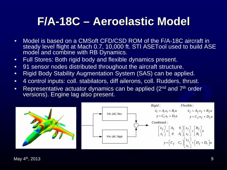
F/A-18C – Aeroelastic Model
F/A-18C Flex
F/A-18C Rigid
: :
:0
0
r r r r f f f f
r r r f f f
f f f f
r r r r
ff r f r
r
Rigid Flexiblex A x B u x A x B uy C x D u y C x D u
Combinedx A x B
ux A x B
xy C C D D u
x
= + = += + = +
= +
= + +
9
• Model is based on a CMSoft CFD/CSD ROM of the F/A-18C aircraft in steady level flight at Mach 0.7, 10,000 ft. STI ASETool used to build ASE model and combine with RB Dynamics.
• Full Stores: Both rigid body and flexible dynamics present. • 91 sensor nodes distributed throughout the aircraft structure. • Rigid Body Stability Augmentation System (SAS) can be applied. • 4 control inputs: coll. stabilators, diff ailerons, coll. Rudders, thrust. • Representative actuator dynamics can be applied (2nd and 7th order
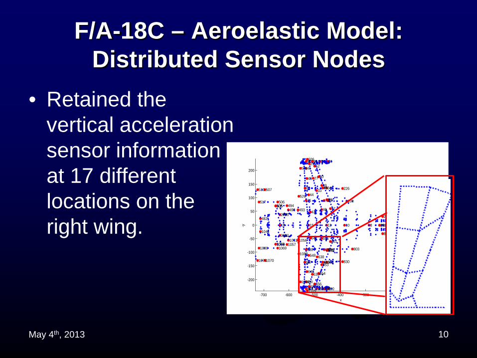
• Retained the vertical acceleration sensor information at 17 different locations on the right wing.
10
-700 -600 -500 -400 -300 -200 -100
-200
-150
-100
-50
0
50
100
150
200
260 260 1 5
296
886
292 292 8
803
200
10
226
830
x
47
651
77
681
86
690
48
652
12
64
668
78
682
688
65
669
49
653
40
645
83
50
654
638
33
686
52
656
27
630
81
43
647
21
625
15
44
648
606
1169
45
649
76
680
80
684
46
650
62
667
531
1094
526
1089
493
1056
498
1061
494
1057
19
2030
3030
506
1069
505 505
1068 1068
507
1070
482
1045
517
1080
513
1076
-y
May 4th, 2013
TECHNICAL REVIEW: MODAL IDENTIFICATION
METHODS
11
May 4th, 2013
Identification Methods
12
• Frequency Domain: Curve fitting Frequency Domain Decomposition (CFDD). – Uses the output power spectral density matrix and its singular
vectors to estimate mode shapes.
• Frequency Domain: Bendat and Piersol Half Power Bandwidth (B&P). – Uses the singular values from the CFDD method to determine the
modal frequency and damping ratio.
• Time Domain: Subspace based system ID (GRA). – Estimate the A and C matrices. – Mode shapes are related to the eigenvectors of A and modified by
the output matrix C.
May 4th, 2013
Classical Approach to Identifying Modal Characteristics
• Based on picking the peaks in a power-spectral density diagram. – These peaks are fit with lower order systems from which the
frequencies and damping can be determined. • Selecting the peaks can be difficult using classical frequency
analysis. • If several signals need to be analyzed, the auto-spectrum and cross-
spectrum plots need to be analyzed for each. – Analyzing the required auto/cross spectrum plots becomes prohibitive
for even a modest number of data signals. • Singular Value Decomposition (SVD) of the power spectral-density
matrix as put forth by Brincker et al. was used to circumvent this potential issue.
Rune Brincker, Lingmi Zhand and Palle Andersen, ‘Modal Identification from Ambient Responses using Frequency Domain Decomposition’, XVIII IMAC, S. Antonio, TX, 2000.
13
May 4th, 2013
Curve fitting Frequency Domain Decomposition (CFDD)
• Create the power spectral density matrix for all output signals. – A unique matrix created for each considered frequency. – Diagonal elements are the auto-spectral density values. – Off-diagonal elements are cross-spectral density values. – Using multiple output signals improves the resolution of
the singular value frequency response. • Perform SVD on each power spectral density matrix. • The resulting frequency domain singular value data
can be used to estimate natural frequency and damping ratios with curve fitting techniques.
14
May 4th, 2013
Curve fitting Frequency Domain Decomposition (CFDD) – cont.
• Fit the peaks of the generated singular value data with an assumed 4th order system (mirrored 2nd order denominator).
• Roots of the 2nd order denominator provide the estimated modal frequency and damping.
15
100 200 300 400 500 600 70010
-6
10-5
10-4
10-3
10-2
10-1
100
Mag
nitu
de
ω (rad/sec)
Auto-Spectral Density
auto-spectral densitycfdd curve fitpeak frequency locationhalf power bandwidth frequency bounds
[ ][ ]1.114,03569.01.114,03569.010749.3
−e
May 4th, 2013
Bendat and Piersol (B&P) • Modal frequency based on the selected peaks in the singular
value data from the CFDD method. • Half power bandwidth used to estimate the damping ratio. • Some restrictions exist in the application of the B&P method.
16
100 105 110 115 120 125 13010
-2
10-1
100
Mag
nitu
de
ω (rad/sec)
Auto-Spectral Density
– Autospectrum of the excitation must be reasonably uniform over the frequency of the normal mode.
– ζ ≤ 0.05 – Analysis resolution bandwidth
must be smaller than the half-power point bandwidth.
– Mode must not heavily overlap with neighboring modes.
𝐵𝑟 = 𝑓2 − 𝑓1 𝑤𝑤𝑤𝑟𝑤 𝐻 𝑓12 = 𝐻 𝑓2
2 =12 𝐻 𝑓𝑟 2
ζ𝑟 =𝐵𝑟2𝑓𝑟
May 4th, 2013
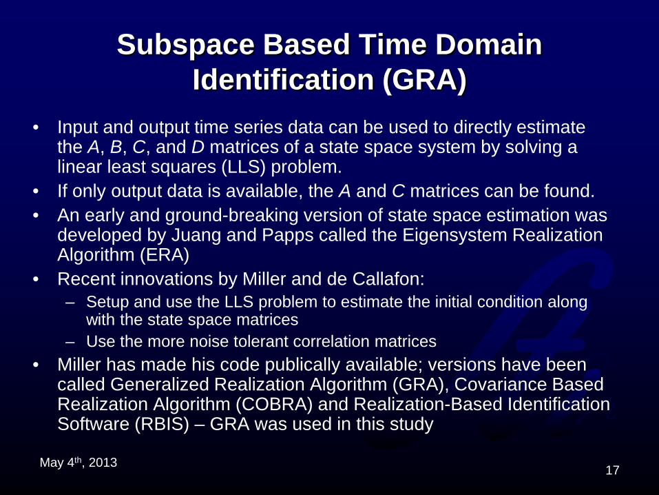
Subspace Based Time Domain Identification (GRA)
• Input and output time series data can be used to directly estimate the A, B, C, and D matrices of a state space system by solving a linear least squares (LLS) problem.
• If only output data is available, the A and C matrices can be found. • An early and ground-breaking version of state space estimation was
developed by Juang and Papps called the Eigensystem Realization Algorithm (ERA)
• Recent innovations by Miller and de Callafon: – Setup and use the LLS problem to estimate the initial condition along
with the state space matrices – Use the more noise tolerant correlation matrices
• Miller has made his code publically available; versions have been called Generalized Realization Algorithm (GRA), Covariance Based Realization Algorithm (COBRA) and Realization-Based Identification Software (RBIS) – GRA was used in this study
17
May 4th, 2013
TECHNICAL REVIEW: MODE SHAPE COMPARISON
18
May 4th, 2013
Complex Mode Shape Estimation
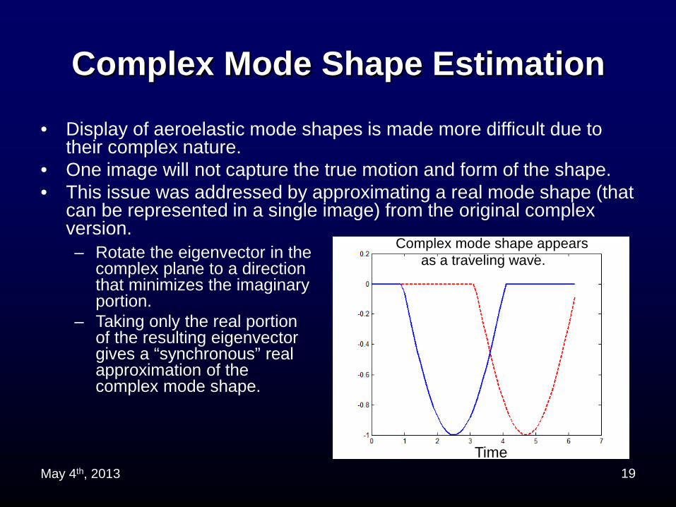
• Display of aeroelastic mode shapes is made more difficult due to their complex nature.
• One image will not capture the true motion and form of the shape. • This issue was addressed by approximating a real mode shape (that
can be represented in a single image) from the original complex version.
19
– Rotate the eigenvector in the complex plane to a direction that minimizes the imaginary portion.
– Taking only the real portion of the resulting eigenvector gives a “synchronous” real approximation of the complex mode shape.
Time
Complex mode shape appears as a traveling wave.
May 4th, 2013
Complex Mode Shape Estimation cont.
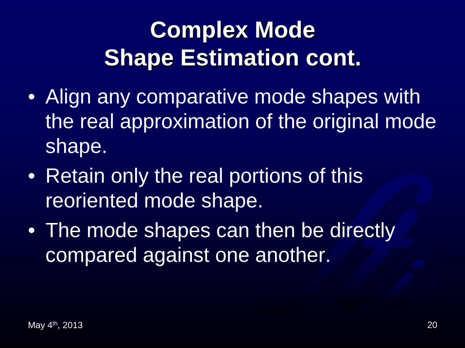
• Align any comparative mode shapes with the real approximation of the original mode shape.
• Retain only the real portions of this reoriented mode shape.
• The mode shapes can then be directly compared against one another.
20
May 4th, 2013
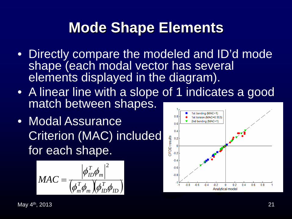
• Directly compare the modeled and ID’d mode shape (each modal vector has several elements displayed in the diagram).
• A linear line with a slope of 1 indicates a good match between shapes. • Modal Assurance Criterion (MAC) included for each shape.
Mode Shape Elements
21
( )( )IDTIDm
Tm
mTIDMAC
φφφφ
φφ2
=
May 4th, 2013
Mode Shape Error
22
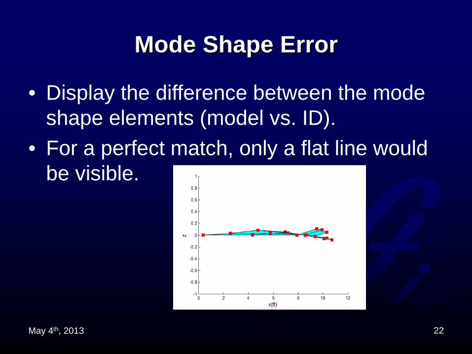
• Display the difference between the mode shape elements (model vs. ID).
• For a perfect match, only a flat line would be visible.
May 4th, 2013
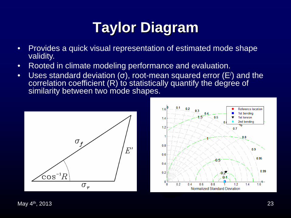
Taylor Diagram
23
• Provides a quick visual representation of estimated mode shape validity.
• Rooted in climate modeling performance and evaluation. • Uses standard deviation (σ), root-mean squared error (E/) and the
correlation coefficient (R) to statistically quantify the degree of similarity between two mode shapes.
May 4th, 2013
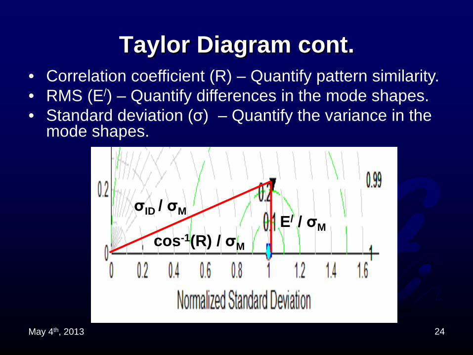
Taylor Diagram cont.
24
• Correlation coefficient (R) – Quantify pattern similarity. • RMS (E/) – Quantify differences in the mode shapes. • Standard deviation (σ) – Quantify the variance in the
mode shapes.
σID / σM E/ / σM
cos-1(R) / σM
May 4th, 2013
TECHNICAL REVIEW: IDENTIFICATION EXAMPLES
25
May 4th, 2013
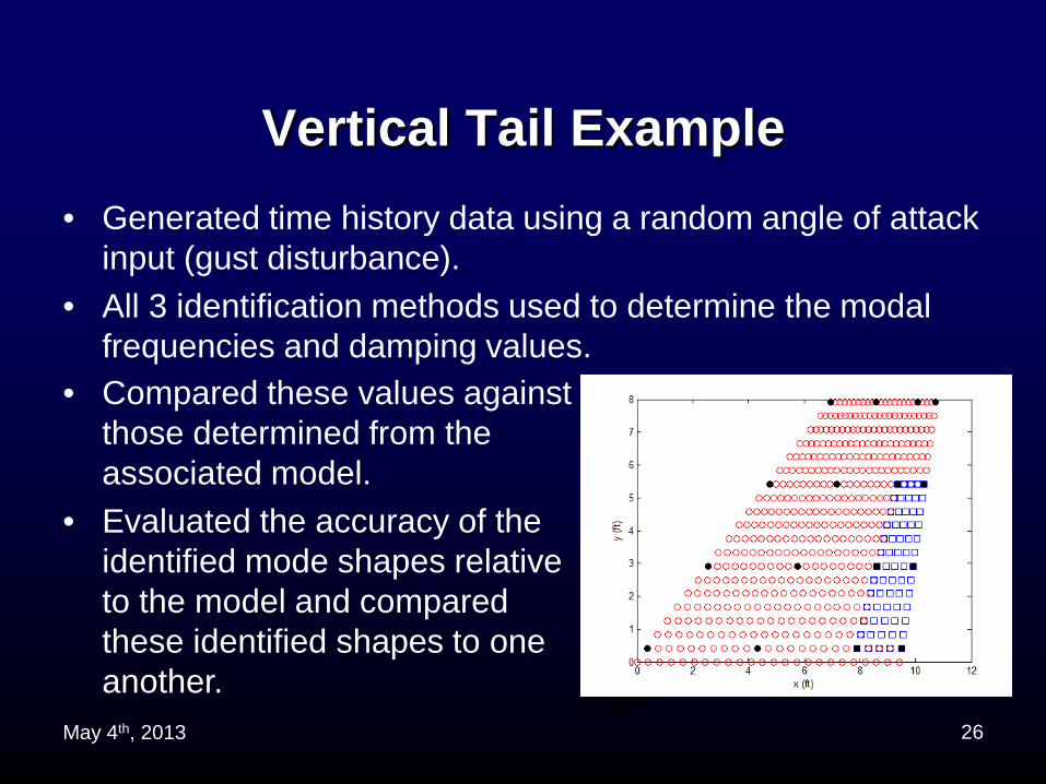
Vertical Tail Example • Generated time history data using a random angle of attack
input (gust disturbance). • All 3 identification methods used to determine the modal
frequencies and damping values.
26
• Compared these values against those determined from the associated model.
• Evaluated the accuracy of the identified mode shapes relative to the model and compared these identified shapes to one another.
May 4th, 2013
Vertical Tail: ID Results
27
Model CFDD Bendat & Piersol GRA
Mode Frequency (rad/s) Damping Frequency
(rad/s) Damping Frequency (rad/s) Damping Frequency
(rad/s) Damping
First bending 114 0.0438 114.08 0.0357 113.47 0.0365 116 0.0194
First torsion 307 0.0243 307.24 0.0198 306.65 0.0191 298 0.0203
Second bending 376 0.000246 375.84 0.0097 377.17 0.0093 375 0.0034
Truth vs. CFDD
Truth vs. GRA
GRA vs. CFDD
May 4th, 2013
Vertical Tail: Mode Shape Metrics
28
CFDD
GRA
1st mode 2nd mode 3rd mode
May 4th, 2013
Vertical Tail: Method Comparison
29
CFDD vs. model
GRA vs. model
CFDD vs. GRA
May 4th, 2013
Vertical Tail Example 1st Bending
30
Frame Model CFDD GRA
May 4th, 2013
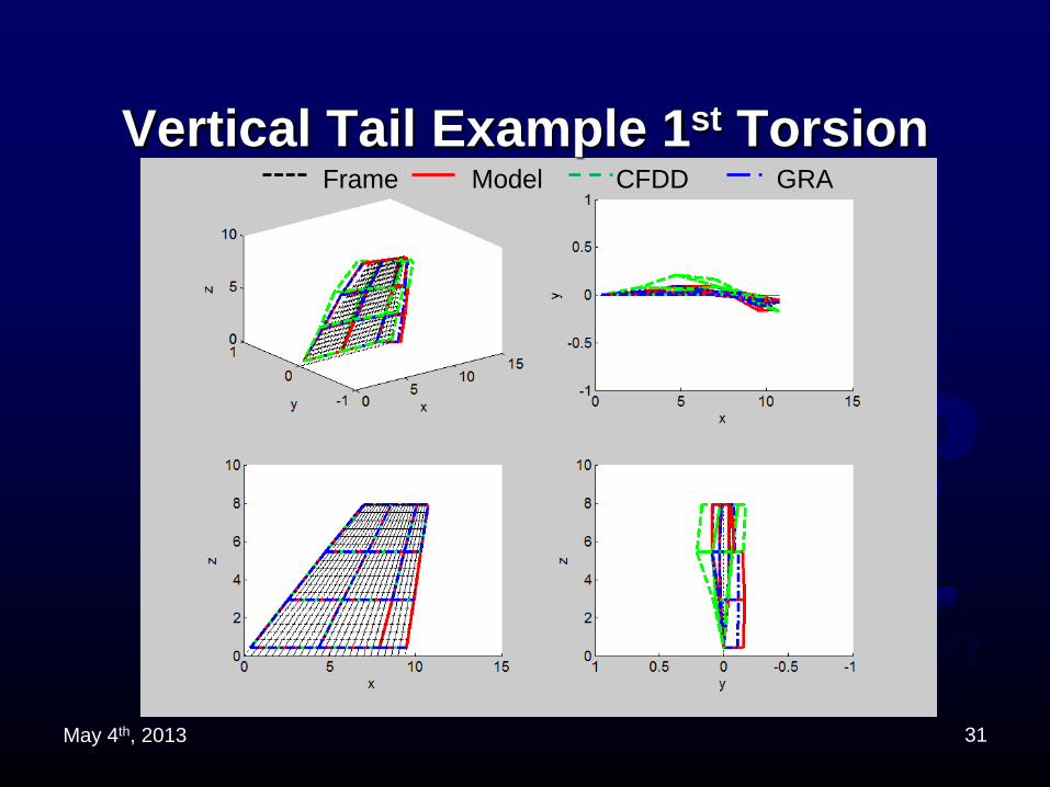
Vertical Tail Example 1st Torsion
31
Frame Model CFDD GRA
May 4th, 2013
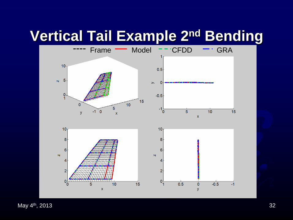
Vertical Tail Example 2nd Bending
32
Frame Model CFDD GRA
May 4th, 2013
REALTIME DEMONSTRATION
33
May 4th, 2013
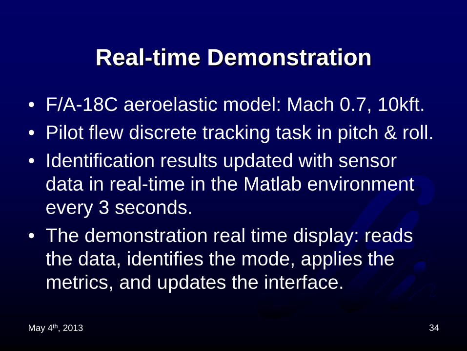
Real-time Demonstration
• F/A-18C aeroelastic model: Mach 0.7, 10kft. • Pilot flew discrete tracking task in pitch & roll. • Identification results updated with sensor
data in real-time in the Matlab environment every 3 seconds.
• The demonstration real time display: reads the data, identifies the mode, applies the metrics, and updates the interface.
34
May 4th, 2013
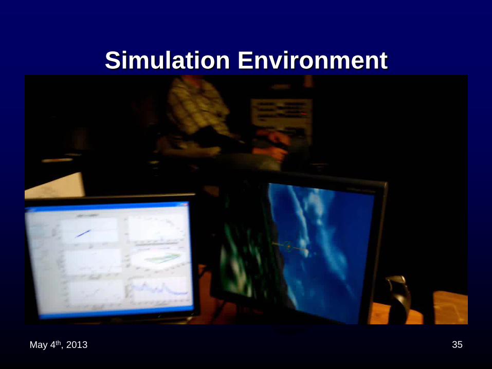
Simulation Environment
35
May 4th, 2013
Real-time Analysis Video
36
May 4th, 2013
Phase I Summary and Conclusions
37
May 4th, 2013
Phase I Summary and Conclusions
• DISPLAYS: Presented a preliminary set of mode shape comparison figures and metrics.
• FEASIBILITY: Each of the 3 identification methods (CFDD, B&P, GRA) were successfully demonstrated and will be carried forward.
• REAL TIME DEMO: Real-time identification of the modal frequency, damping ratio and mode shape was successfully demonstrated using STI’s fixed based simulator and the F/A-18C aeroelastic model.