Real-Time Automated Modeling and Controlof Self-Assembling Systems
Gregory Mermoud, Massimo Mastrangeli, Utkarsh Upadhyay and Alcherio Martinoli
Abstract— We present the M3 framework, a formal andgeneric computational framework for modeling and controllingstochastic distributed systems of purely reactive robots in anautomated and real-time fashion. Based on the trajectories ofthe robots, the framework builds up an internal microscopicrepresentation of the system, which then serves as a blueprintof models at higher abstraction levels. These models are thencalibrated using a Maximum Likelihood Estimation (MLE)algorithm. We illustrate the structure and performance ofthe framework by performing the online optimization of abang-bang controller for the stochastic self-assembly of water-floating, magnetically latching, passive modules. The exper-imental results demonstrate that the generated models cansuccessfully optimize the assembly of desired structures.
I. INTRODUCTION
The controlled formation of structures and patterns is afundamental task of distributed robotic systems. In particular,self-assembling systems come in several varieties, which canbe classified based on, for instance, the role of energy andinformation, the control modality (e.g., centralized versusdistributed), the size of the components and their type—active (e.g., autonomous robots) or passive (e.g., MEMS,macromolecules). Overall, the ongoing convergence betweenrobotic minimalism and the increasing sophistication ofmicro/nanosystems allows one to envision a unifying per-spective for self-assembling systems across scales [1]. Whilesoundly grounded in current technological trends and sup-ported by a few remarkable theoretical frameworks, suchappealing perspective still lacks substantial and consolidatedmodeling methodologies, as compared to the wide-rangingefforts in components development [2], [3].
Among the approaches to model robotic systems, hybridautomata stand out for capturing both continuous and discretestate variables [4]. When dealing with distributed systems,one often uses a combination of multiple abstraction levels,which often includes probabilistic and graphical models [5].However, most modeling methodologies are not sufficientlysystematic to be carried out in an automatic fashion [5], [4],[6]. Alternative methods for automated model constructionadopt completely different strategies based on evolutionarycomputation [7]. In spite of their attractive flexibility andversatility, these methods are computationally expensive, andthey yield gray-box models whose structure and parameters
The authors are with the Distributed Intelligent Systems and Al-gorithms Laboratory (DISAL), School of Architecture, Civil and En-vironmental Engineering, Ecole Polytechnique Federale de Lausanne.Gregory Mermoud and Massimo Mastrangeli are sponsored by the Nano-Tera.ch research initiative in the framework of the SelfSys [email protected]
are difficult to anchor back to the original system. In partic-ular, they rely on a single level of abstraction, even in thecontext of collective systems (e.g., biological and chemicalreaction networks [8], [9]), thereby precluding any mappingbetween microscopic and macroscopic states.
The control of self-assembling system has been tackledby several previous works, which generally rely on controlof local interactions among building blocks [10], [11], [12].Napp et al. [13] control the formation of heterodimers byadjusting only global parameters of the system (i.e., lightintensity); however, the underlying model is designed andcalibrated manually, and they do not investigate the formationof more complex structures.
In this work, we present the M3 framework, a formal andgeneric computational framework that allows for the auto-matic construction and calibration of models of distributedstochastic systems of purely reactive robots. Based on ageneric microscopic representation of a system, the frame-work generates an associated Chemical Reaction Network(CRN) model in real-time, and allows for an optimal, globalcontrol of the system as well. We hereby experimentallydemonstrate the performance of the M3 framework bymodeling and optimizing, in real time and without humansupervision, a stochastic self-assembling system of water-floating passive modules.
II. EXPERIMENTAL SETUP
We study the stochastic self-assembly of target structuresof 3-cm-sized water-floating devices, denoted as blocks here-after, within a circular water-filled tank. The experimentalsetup consists of the tank, with six inlets and four outlets con-nected to four diaphragm pumps (see Fig. 1(a)), four blocks,an overhead camera and a workstation. The cuboidal, centro-symmetric blocks are passive and endowed with four SmCopermanent magnets (one on each side’s center) for mutualaggregation, as well as with a visual marker for trackingpurposes (see Fig. 1(b)). The weight of each block (about17.3 g, compared to a buoyancy limit of 21.9 g) was trimmedfor reliable floatation. The blocks are not self-locomoted;instead, they are stirred by the fluid flow produced within thetank by the peripheral pumps. As a result, the blocks describetrajectories with well-defined geometric features, yet with astrong stochastic component [14].
The tank, of approximately 30 cm in diameter, has fourinlets perpendicular to the wall and other two almost tangen-tial, allowing to create flows with both radial and circularcomponents. Additionally, the four outlets are placed at thebottom of the tank so as not to interfere with the surface flow.
2012 IEEE International Conference on Robotics and AutomationRiverCentre, Saint Paul, Minnesota, USAMay 14-18, 2012
Fig. 1. The experimental setup: (a) Water-filled tank with 6 inlets (4 orthogonal and 2 tangential to the wall); (b) Internal details of a water-floatingblock, including the latching mechanism composed of four permanent magnets with different pole orientation—north-south (NS) and south-north (SN),respectively; (c) Real-time visual tracking of four blocks during an experiment (the blue lines show a short history of the trajectory of each block).
Each pump’s flow rate can be controlled individually up toa maximal value of 600 ml/min. This flexible configurationallows us to investigate a variety of different flow patternsand associated block trajectories. Indeed, perpendicular inletsgenerate irregular trajectories, and induce block collisions inthe middle of the tank, but they exhibit dead spots near thewalls. Conversely, tangential inlets generate circular flowsthat prevent dead spots, but lead to regular, closed trajectorieswhich do not favor collisions.
The combined effects of mutual magnetic forces and blockshape geometry lead to the precise pair-wise self-alignmentof blocks upon close proximity (about 0.5 cm), when nothampered by fluidic drag forces. In fact, the interblockbonds were designed to be reversible, as depending on theinterplay between the magnitude of the magnetic (about16 mN per bond according to FEM simulations) and thelocal hydrodynamic forces acting on the blocks, the latterbeing modulated by the fluid flow regimes. As a result, thestability of all the assembled block structures correspondingto local system energy minima could be controlled by themodes of fluidic stirring in the tank, whereas the 2-by-2square structure—labelled D in Fig. 2 and corresponding tothe global system energy minimum—was irreversible andacted as absorbing state in the system dynamics.
To monitor the evolution of the system in real time, weuse an overhead camera to track a two-color passive markerlocated at the top of each block. SwisTrack [15], an open-source software package developed in our laboratory, allowsus to track the pose of the blocks. Both their position (x,y)and orientation (θ) are logged in real time at a rate ofapproximately 30 Hz1. These data are then transmitted tothe modules responsible for the construction of the modeland the optimization, described in sections IV and V.
III. PROBLEM STATEMENT
All feasible structures formed by the assembly of four ofour blocks are reachable and can be enumerated (see Fig. 2).In a well-mixed system, each structure has an intrinsic
1The sampling period (about 33 ms) is much smaller than the averageinter-collision time, which is around 1.15 s.
C1 C2
A B
F1 F2 F3
E D
reac&ons leading to E
other reac&ons
2 2
2
2 2
Fig. 2. Graphical representation of all assemblies that can be formed outof four blocks and the forward reactions that lead to them. Chiral copiesof assemblies F1 and F3 are not included. The shaded rectangles indicateassemblies with the same connection topology (using a 4-neighbors topol-ogy). Black arrows denote the reactions that lead to the target structure E,whereas gray arrows other forward reactions in the system. For readability’ssake, reverse reactions and stoichiometric factors equal to 1 are omitted.
probability of being formed, which depends not only on itsown geometry, but also on the parameters of the system. Forinstance, the assembly A is unlikely to be observed in a smalltank because of the high probability of collision between theblocks.
In this work, we consider a non-well-mixed system(see [16] for more details about this type of systems), whichallows us to further tune the probabilities of structure for-mation by optimizing dynamically the control parameters ofthe system (e.g., those governing the agitation of the system).More formally, the research question that we address in this
4267
paper is the following: Given a stochastic multi-unit systemwith a finite set of agitation modes M = {m0, . . . ,mn},what is the mode mi to be selected at time t that minimizesthe time to form a given target structure T ?
In the present case, we consider only two modes ofagitation (as in a bang-bang controller) corresponding totwo different pump configurations that lead to differentagitation schemes. In mode m0, the fluid flow inducessmooth and regular block trajectories and only marginaldifferences in their relative velocities, thereby allowing fora high stability of the formed aggregates but relatively fewinteractions. In mode m1, the blocks exhibit a much moreerratic movement, dominated by the stochastic perturbationsof the water surface (Faraday waves) caused by pumps-induced tank vibrations. The consequently higher kineticenergy of the blocks increases the collision rate, but alsothe instability of the aggregates.
IV. MODELING FRAMEWORK
In this work, our methodology makes the fundamentalassumption that the robots are strictly reactive, that is,all behavioral changes can be interpreted as the result ofinteractions with other robots or with the environment. Acorollary of this assumption is that one can associate eachbehavior of the robot to some condition on its interactionconfiguration. Indeed, when designing a robot’s controller,one naturally arranges the different interaction configurationsthat the robot can be in into classes indexed by a set ofbehaviors. For instance, the designer can group all situationsin which the robot is close to another robot, and associate theresulting class to a obstacle avoidance behavior. Followingthis methodology, the controller of each robot naturallyreflects the most important states of the robot. As a result,one can use the robot’s controller as a blueprint to constructa meaningful partition of the continuous phase space, andthereby deriving models at higher abstraction levels (see forinstance [5]). This approach opens up new opportunities forautomating model construction and calibration.
We hereby rely on a computational framework, called theM3 framework, which allows for the automatic constructionof models of a multi-robot system. The global structure ofthis framework is depicted in Fig. 3. The general idea ofour approach is that we observe (or simulate) an existingsystem, and the model is built based on the observations(i.e., trajectories) collected during these experiments (or sim-ulations). Internally, the framework builds up a microscopicrepresentation of the system based on these observations aswell as on a list of interactions of interest specified by theuser. This representation, called the Canonical MicroscopicModel (CMM), is a formal and generic description of areactive multi-unit system, and it serves as a blueprint forthe construction of a macroscopic model, specified using theChemical Reaction Network (CRN) formalism. Finally, ateach time step, the optimal mode of agitation is determinedusing the optimization scheme described in Section V, andtransmitted to the (real or simulated) actuators.
Tracking software(SwisTrack)
CanonicalMicroscopic
Model (CMM)
ChemicalReaction
Network (CRN)
Optimization(Policy Iteration)
Pumps
User
Wat
er-fi
lled
tank
and
bloc
ksO
verh
ead
cam
eratrajectories
events
state graph
optimal mode
interactions
targetassem
bly
configuration
fluid
flow
Fig. 3. Overview of the M3 framework as deployed in this study, andthe different types of information flowing between its constitutive modules.Gray-shaded nodes are computational entities whereas other nodes arephysical entities. Dashed arrows denote flows that are not automated, butneed to be performed only once prior to the experiment. Note that theclosed-loop control is completely automated.
Hereafter, we provide a brief summary of the theoreticalfoundations of this framework. A more detailed descriptionwill be published elsewhere.
A. Canonical Microscopic Model (CMM)
We define our system as a set of coupled hybrid au-tomata [17], called particles that interact through a set ofinteractions I = {I1, . . . , It} (see Definition 1). Each parti-cle in the set P = {P1, . . . , Pm} represents a robot in thetarget system. The set P may be partitioned into an arbitraryset of classes of particles Ci (such that
⋃i Ci = P), which
denote particles that have similar control graphs (see below).The state of each robot has two distinct components: (i) ann-dimensional continuous component ~x = [x1, . . . , xn]T ∈X that typically denotes the physical state of the particle(e.g., its position, orientation and velocity in physical space,its temperature, its battery level, etc.)2, and (ii) a discrete
2We write Xi = {x1,i, . . . , xn,i} the set of state variables of particle Pi.
4268
component ξ ∈ V that denotes the logical state of the particle,called control mode, that is, a vertex of the finite directedmultigraph G = (V, E), called the control graph of P . Theedges in E are called control switches. Most importantly, eachcontrol mode ξj is labeled with a unique function φj : I →N0, called an interaction configuration. The function φj(I)denotes the number of interactions of type I that are activein mode ξj . In other words, each control mode is associatedto a unique interaction configuration, and vice versa, suchthat there exists a one-to-one map Φ : V → {φ1, . . . , φk}.Definition 1 [Interaction] An interaction I is defined as atriplet (Ci, Cj , cond) where Ci and Cj are two classes ofparticles that may interact through I; the predicate conddescribes the conditions in which I is active, and whosefree variables are in Xi′ ∪ Xj′ , with i′, j′ the indices of theinteracting particles.
The CMM exhibits a few key properties: (i) it describes agiven distributed system as a set of coupled hybrid automata,thereby allowing for a natural coupling between the contin-uous and discrete components of the state space; (ii) theunderlying assumptions of the CMM allow the algorithmicconstruction of the control space V of its constitutive par-ticles solely based on their trajectories in the continuousstate space X; (iii) because the control modes in V aremapped to a unique interaction configuration, they forma partition of the continuous phase space S, that is, thecontinuous space of the entire system; (iv) ultimately, bya proper aggregation of those control modes, one can obtaina more tractable and meaningful set of metastates, which wedenote q1, . . . , qr. Importantly, this process of aggregationis precisely the mental process carried out by the designerof a robotic system. The latter metastates are the basis foran algorithmic conversion of any CMM into an equivalentmacroscopic representation based on the CRN formalism.
As mentioned earlier, the control space is built iterativelyas observations of the system are collected (see Algorithm 1):starting from an initial control space V = {0}, whichcontains only a non-interacting mode, each newly observedcontrol mode ξ > 0 is appended to V . As depicted byFig. 3, the construction of the CMM is based on trajectoriescollected either in simulation or in real experiments. Fromthe point of view of the framework, the nature of thetrajectories has no importance.
B. From the CMM to Macroscopic Models
The formalism of hybrid automata is interesting from atheoretical point of view, yet not very practical numerically.To enhance its applicability, we hereafter introduce the notionof Chemical Reaction Network (CRN), and we show howone can automatically convert the CMM into a CRN.
The general idea of our approach is to use the controlgraph G of the particles of the system as a blueprint of themodel structure. It is often necessary to refine the resultingmodels a posteriori, in order to account for hidden controlmodes, which are relevant to either the performance metricor the accuracy of the model. For instance, in aggregation
Algorithm 1 Iterative construction of the control space VRequire: Vi = {0},∀i ∈ {1, . . . ,m}
while t < tend dofor each Pi ∈ P do
Update ~xi(t+ ∆t) according to observationsif an interaction has occurred/ended then
Compute new interaction configuration φ′
if ¬∃ξ′ ∈ Vi s.t. Φ(ξ′) = φ′ thenCreate ξ′ and updates Φ s.t. Φ(ξ′) = φ′
Append ξ′ to Vi and e = (ξi, ξ′) to Ei
end ifξi(t+ ∆t)← ξ′
end ifend fort← t+ ∆t
end while
scenarios [18], [19], pieces of information that are critical tothe evaluation of the performance metric, such as the size orthe shape of the aggregates, are not available to the robots(and therefore not reflected in their controller). To keep trackof these global arrangements of interaction, we introduce thenotion of interaction graph and aggregate.Definition 2 [Interaction Graph] The interaction graph Gint =(P, E int) is a graph whose edge set E int is given by (Pi, Pj) ∈E int iff ∃I ∈ I such that Pi and Pj interact through I .
Definition 3 [Aggregate] We note A = {A1, . . . , Aq} theset of all feasible aggregates, that is, connected subgraphsof the interaction graph Gint.
Definition 4 [Chemical Reaction Network] Similarly toprevious works [20], [21], we define a CRN N = (R,S) asa set of N reactions R = {R1, . . . , RN} acting on a finitenumber M of species S = {S1, . . . , SM}. Each reaction Ris defined as two vectors of nonnegative integers specifyingthe stoichiometry of the reactants, ~rR = [rR,1, . . . , rR,M ],and the products, ~pR = [pR,1, . . . , pR,M ], respectively. Thestoichiometry denotes how many copies of a given reactantor product is required or produced, respectively, when areaction takes place. For example, assume a CRN with S ={A,B,C}, the reaction A + 3B ⇀ A + 2C is representedby the following vectors:
~r = [1 3 0]
~p = [1 0 2]
The CRN being a population model, it keeps track of howmany individuals of each species are present in the systemat a given time. The state of the CRN is therefore given bythe vector ~X ∈ NM
≥0, whose elements specify the number ofindividuals of each species. A reaction R may occur iff thenumber of reactants is sufficient, that is, ~X ≥ ~rR element-wise. When reaction R occurs, the new state ~X ′ is simplygiven by:
~X ′ = ~X − ~rR + ~pR = ~X + ~νR (1)
with ~νR the population change caused by reaction R.
4269
1 The M3 Framework for Distributed Robotic Systems 5
t = t0A
p1 p2 p3
S0
Control Graph
1S0
CRN
t = t1 > t0A
p1 p2 p3 S0
A1
Control Graph
1S0
2A1
21
CRN
t = t2 > t1A
p1 p2 p3
S0
A1
A2
Control Graph
1S0
2A1
2A11A2
21
1
1
1
CRN
Continuous Component Discrete Component
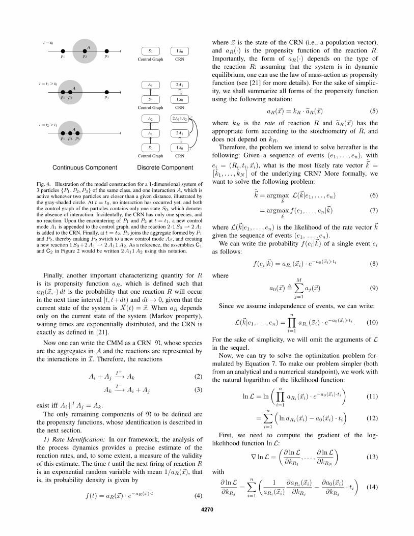
Fig. 1.1 Illustration of the model construction for a 1-dimensional system of 3 parti-cles {p1, p2, p3} belonging to the same class and one interaction A, which is active whenever twoparticles are closer than a given distance. At t = t0, no interaction has occurred yet, and both thecontrol graph of the particles contains only one state S0, which denotes the absence of interaction.Incidentally, the CRN has only one species, and no reaction. Upon the encountering of p1 and p2at t = t1, a new control mode A1 is appended to the control graph, and the reaction 2 ·1S0 ⇀ 2A1 isadded to the CRN. Finally, at t = t2, p3 joins the aggregate formed by p1 and p2, thereby making p2switch to a new control mode A2, and creating a new reaction 1S0 +2A1 ⇀ 2A11A2.
Component 3 (Initial, invariant, and flow conditions). Three vertex-labeling func-tions init, inv, and f low that assign to each control mode ξ ∈ V three predicates.Each initial condition init(ξ ) is a predicate whose free variables are from
⋃pi∈PXi.
Each invariant condition inv(ξ ) is a predicate whose free variables are from⋃
pi∈PXi.The flow conditions f low(ξ ) are predicates that take the form of a collection ofstochastic processes
{Y ξ
1 (t), . . . ,Y ξn (t)
}ξ∈V. In other words, the trajectory xi(t)
along the i-th dimension of state space is a realization of some stochastic pro-cess Y ξ
i (t). More formally, if we use the following definition of a stochastic process:
YX (t) = f (X , t) (1.2)
where X is a stochastic variable, and f some time-dependent mapping between Xand the stochastic process YX , then, on inserting for X one of its possible values x,we obtain:
Fig. 4. Illustration of the model construction for a 1-dimensional system of3 particles {P1, P2, P3} of the same class, and one interaction A, which isactive whenever two particles are closer than a given distance, illustrated bythe gray-shaded circle. At t = t0, no interaction has occurred yet, and boththe control graph of the particles contains only one state S0, which denotesthe absence of interaction. Incidentally, the CRN has only one species, andno reaction. Upon the encountering of P1 and P2 at t = t1, a new controlmode A1 is appended to the control graph, and the reaction 2·1S0 ⇀ 2A1
is added to the CRN. Finally, at t = t2, P3 joins the aggregate formed by P1
and P2, thereby making P2 switch to a new control mode A2, and creatinga new reaction 1S0+2A1 ⇀ 2A11A2. As a reference, the assemblies C1
and C2 in Figure 2 would be written 2A11A2 using this notation.
Finally, another important characterizing quantity for Ris its propensity function aR, which is defined such thataR(~x, ·) dt is the probability that one reaction R will occurin the next time interval [t, t+dt) and dt→ 0, given that thecurrent state of the system is ~X(t) = ~x. When aR dependsonly on the current state of the system (Markov property),waiting times are exponentially distributed, and the CRN isexactly as defined in [21].
Now one can write the CMM as a CRN N, whose speciesare the aggregates in A and the reactions are represented bythe interactions in I. Therefore, the reactions
Ai +AjI+
−−→ Ak (2)
AkI−−−→ Ai +Aj (3)
exist iff Ai ‖I Aj = Ak.The only remaining components of N to be defined are
the propensity functions, whose identification is described inthe next section.
1) Rate Identification: In our framework, the analysis ofthe process dynamics provides a precise estimate of thereaction rates, and, to some extent, a measure of the validityof this estimate. The time t until the next firing of reaction Ris an exponential random variable with mean 1/aR(~x), thatis, its probability density is given by
f(t) = aR(~x) · e−aR(~x)·t (4)
where ~x is the state of the CRN (i.e., a population vector),and aR(·) is the propensity function of the reaction R.Importantly, the form of aR(·) depends on the type ofthe reaction R: assuming that the system is in dynamicequilibrium, one can use the law of mass-action as propensityfunction (see [21] for more details). For the sake of simplic-ity, we shall summarize all forms of the propensity functionusing the following notation:
aR(~x) = kR · aR(~x) (5)
where kR is the rate of reaction R and aR(~x) has theappropriate form according to the stoichiometry of R, anddoes not depend on kR.
Therefore, the problem we intend to solve hereafter is thefollowing: Given a sequence of events (e1, . . . , en), withei = (Ri, ti, ~xi), what is the most likely rate vector ~k =[k1, . . . , kN
]of the underlying CRN? More formally, we
want to solve the following problem:
~k = argmax~kL(~k|e1, . . . , en) (6)
= argmax~k
f(e1, . . . , en|~k) (7)
where L(~k|e1, . . . , en) is the likelihood of the rate vector ~kgiven the sequence of events (e1, . . . , en).
We can write the probability f(ei|~k) of a single event eias follows:
f(ei|~k) = aRi(~xi) · e−a0(~xi)·ti (8)
where
a0(~x) ,M∑
j=1
aj(~x) (9)
Since we assume independence of events, we can write:
L(~k|e1, . . . , en) =n∏
i=1
aRi(~xi) · e−a0(~xi)·ti . (10)
For the sake of simplicity, we will omit the arguments of Lin the sequel.
Now, we can try to solve the optimization problem for-mulated by Equation 7. To make our problem simpler (bothfrom an analytical and a numerical standpoint), we work withthe natural logarithm of the likelihood function:
lnL = ln
( n∏
i=1
aRi(~xi) · e−a0(~xi)·ti)
(11)
=n∑
i=1
(ln aRi
(~xi)− a0(~xi) · ti)
(12)
First, we need to compute the gradient of the log-likelihood function lnL:
∇ lnL =
(∂ lnL∂kR1
, . . . ,∂ lnL∂kRN
)(13)
with
∂ lnL∂kRj
=n∑
i=1
(1
aRi(~xi)
∂aRi(~xi)
∂kRj
− ∂a0(~xi)
∂kRj
· ti)
(14)
4270
where
∂aRi(~xi)
∂kRj
=∂kRi
· aRi(~xi)
∂kRj
=
{aRi
(~xi) if Rj = Ri
0 otherwise(15)
and
∂a0(~xi)
∂kRj
· ti =∂aRj
(~xi)
∂kRj
· ti = ti · aRj(~xi) (16)
Replacing these terms into Equation 14, we obtain
∂ lnL∂kRj
=n∑
i=1
(1Ri=Rj
kRi
− ti · aRj(~xi)
). (17)
where 1Ri=Rjis the indicator function. A local extremum
of the function lnL corresponds to a zero of the gradient
∇ lnL =(0, . . . , 0
)(18)
which is equivalent to writing
kj =
∑ni=1 1{Ri=Rj}∑n
i=1
(ti · aRj
(~xi)) (19)
for j = 1, . . . , N . Importantly, the rate of reaction R = Rj
also depends on events that do not involve R. For this point tobe a maximum of lnL, we need the Hessian matrix H(lnL)to be negative-definite, which can be easily demonstrated.
If the waiting times of a reaction are not exponentiallydistributed, it means either that the underlying reaction isnot memoryless, or that some relevant features have beenneglected (in particular, spatiality). In such cases, one wouldneed to either (i) use an appropriate simulation scheme, inorder to capture the characteristic distribution of the waitingtimes, or (ii) modify the structure of the model to mitigate theimpact of this reaction (e.g., by augmenting the state spaceof the model with states that account for previous reactionpartners, as proposed by Napp et al. [16]). However, suchresearch avenues are beyond the scope of this paper, andwe do not perform any further refinement of the resultingmodels.
V. OPTIMIZATION
As stated in Section III, we aim at favoring the formationof a predefined target structure T . We show how this problemis equivalent to another well-known problem, that is, thesolving of Markov Decision Processes (MDPs). Indeed,forming the structure T is equivalent to attaining a targetpopulation ~xt = (xt,1, . . . , xt,M ) such that
xt,i =
{1 if Si = T,
0 otherwise.(20)
Therefore, our problem consists in determining themode ms ∈M to be selected given an initial population ~xssuch that the expected time to reach ~xt is minimized.
For each mode m ∈ M, we have an estimate of thepropensity function a
(m)R (~x) for each reaction R ∈ R.
Denote k(m)ij = a
(m)R (~xi) the rate of the reaction R whose
associated population change is ~νR = ~xj − ~xi if mode m isselected. Furthermore, we define the following quantities:
λ(m)i =
∑
j
k(m)ij , p
(m)ij =
k(m)ij
λ(m)i
. (21)
Note that each state has only one optimal choice for themode which minimizes the expected time it takes to reachthe target population ~xt and this choice is independent of thepast states or how much time has been spent in the presentstate.
Denote by Tij the expected time it takes the system toattain the population ~xj for the first time if it starts withpopulation ~xi and makes optimal choice for the mode at eachsubsequent state. Hence, Tij is the optimal first-passage timefrom population ~xi to ~xj . We consider the target population~xt to be an absorbing state, which is reasonable if theexperiment halts as soon as the desired state is attained.
Now for Tij to be optimal, it is easy to show that theymust satisfy:
Tit = minm∈M
∑
j 6=i,t
p(m)ij · Tjt +
1
λ(m)i
(22)
This equation reiterates the Markov property of the system,that is, the expected time to reach population ~xt is the sumof expected time to reach the state via any of its neighbor(except ~xt itself) and the expected time to exit the presentstate. N−1 such equations can be written for different i 6= tfor Tit.
This equation is a Bellman equation corresponding to ourMarkov Decision Process [22], and can be solved to obtainthe expected times and the optimal modes for each popula-tion state. We used the Policy Iteration method to solve theequations in our case. The optimization is performed uponeach aggregation or disaggregation event observed in thesystem, and every 10 seconds otherwise. Previous solutionsare kept in memory, and used for initializing the subsequentiterations to speed up the optimization process.
VI. RESULTS AND DISCUSSION
To demonstrate the effectiveness of our automatic modelbuilding framework and the relevance of our optimizationalgorithm, we performed four distinct experiments using theassembly E depicted in Fig. 2 as target structure and withdifferent control algorithms: (I) mode m0 only, (II) mode m1
only, (III) randomized control, where the two modes alternaterandomly with an average switching period of 15 s, and (IV)optimized control, in which the optimizer selects the mostappropriate mode of agitation as a function of the currentstate of the system and of the current state of the model.The performance of the system is given by the time of thefirst occurrence of the assembly E, denoted as first-passagetime, and bounded by the maximal duration of the run.
Each experiment consists of a series of 40 runs of 30minutes each. Each run starts with all blocks being isolatedand at random locations. In experiment IV, the optimizationrelies on an initial model based on the observations made
4271
during two series (one per mode) of 10 runs of 5 minuteseach. However, as explained earlier, the model is constantlyenhanced, both qualitatively (e.g., if a new type of aggregateis discovered) and quantitatively (i.e., the reaction rates areadjusted) as the experiment progresses.
The underlying models are constructed based on a singleinteraction that is active between two blocks when they areboth close to each other and appropriately aligned. As aresult, several assemblies that are actually distinct from eachother cannot be discriminated by the model, as seen by Fig. 2.
The choice of E as target structures was made because itcan be univocally mapped to a unique species of the CRN,and it can be formed out of both C1 and C2. Indeed, theassembly D can also be univocally mapped to a uniquespecies of the CRN, but cannot be formed out of C2.As a result, the optimizer cannot effectively decide whichmode of agitation should be applied when a trimer (i.e., C1
or C2) is present since these two assemblies are topologicallyundistinguishable. Note however that this is by no meansan intrinsic limitation of our methodology, but rather aconsequence of the simplicity of the underlying model.
First, as shown in Fig. 5, our results support the intu-itive argument that self-assembly, as any self-organized pro-cess, requires a subtle interplay between “exploitation” and“exploration”—as expressed by the low-agitation m0 and thehigh-agitation m1, respectively. Indeed, both experiments Iand II exhibit poor performance even as compared to thenaive strategy that alternates between the two modes ofagitation randomly. More importantly, our results show thatone can drastically improve the performance of the system byoptimizing the mode of agitation as a function of the system’sstate. Indeed, we observe a 40% and 66% decrease of theaverage and median first-passage time, respectively, underoptimized control. When observing the system (Fig. 6), itlooks like the strategy adopted by the optimizer is intuitive:the mode m0 (low agitation) is active as long as assembliesthat may lead to E (i.e., assemblies A, B, C1, and C2) arepresent, and switches to the mode m1 (strong agitation) assoon as some incorrect tetramer is formed. However, theoptimization also exhibits some interesting and less obviousbehaviors. First, when only single blocks are present inthe system, it sets the mode m1 so as to favor mutualcollisions. Upon the formation of a dimer B, the systemmay switch to mode m0 in order to preserve it; however,while most reactions have clearly different rates for m0
and m1 (typically, one order of magnitude or more), thereaction A+B→ Cx exhibits relatively similar rates in eithermode, thereby allowing for a dynamic switching betweentwo behaviors, as a function of the time spent in each. Forinstance, the optimizer may select mode m0 in order toconserve the formed dimer, but as the experiment progresses,the reaction rate of trimer creation in mode m0 decreases,until it becomes smaller than the rate associated to mode m1,thereby leading to the selection of the latter. This type ofadaptive behavior is a built-in feature of our automatedmodeling approach, which is usually obtained using ad-hoclearning strategies (e.g., reinforcement learning) elsewhere.
8 occurences
Firs
t−pa
ssag
e ti
me
to E
[s]
Mode 0 Mode 1 Random Optimized0
500
1000
1500
Fig. 5. Box plot of the first-passage time to the target structure Eobtained over 40 runs of 30 minutes each for experiments I to IV. Oneach box, the central mark is the median, the edges of the box arethe 25th and 75th percentiles, the whiskers extend to the most extremedata points not considered outliers, and outliers are plotted individually.Both experiments I (mode 0 only) and II (mode 1 only) exhibit a poorperformance due to the unfavorable exploration vs exploitation balance whenusing a unique mode of agitation. The mean/median first-passage time ofthe optimized experiment (IV) is 524/205 seconds versus 930/612 secondsfor the randomized experiment (III). A Mann-Whitney test rejects the nullhypothesis that these two distributions of first-passage times are from thesame distribution with equal medians with a p-value of 5.8 · 10−3.
VII. CONCLUSION AND FUTURE WORK
In this paper, we introduced the M3 framework, a genericcomputational framework for the automatic, real-time mod-eling and control of stochastic and reactive multi-robotsystems. We briefly summarized the theoretical foundationsof the framework, and we demonstrated its relevance bydeploying it for modeling and controlling the stochastic self-assembly of 3-cm-sized passive water-floating blocks. Wedescribed how the resulting models can be used to optimizea bang-bang controller, and our results show a significantimprovement of the performance of the system with respectto strategies based on single modes of agitation or a randomswitching between the modes.
In future, we plan to investigate the use of more complexmodels (by adopting a 8-neighbors topology, for instance),and how they may enhance the overall performance of thesystem. Also, we aim at demonstrating the generality and thescalability of our approach by applying it to larger ensem-bles and other platforms. The strict requirement of perfectobservability is currently an obstacle to the applicability ofthe M3 framework in some circumstances (e.g., microscaleself-assembly), but future theoretical developments and theuse of more advanced machine learning methods shall allowfor relaxing this requirement [9].
VIII. ACKNOWLEDGEMENTS
The authors would like to acknowledge Emmanuel Drozand Maria Boberg for technical support as well as SvenGowal and Jose Nuno Pereira for useful discussion. Fur-thermore, we would like to acknowledge the Nano-Tera.chresearch initiative, which partly sponsored this research inthe context of the SelfSys project.
4272
t = 0 sec t = 14 sec t = 24 secmode 1 mode 1 mode 0
2A → B A + B → C2
t = 32 sec t = 34 sec t = 78 secmode 1 mode 0 mode 1
A + C2 → F1 F1 → A + C1 A + C1 → F3
t = 83 sec t = 98 sec t = 146 secmode 1 mode 0 stop
F3 → 2 B and B → 2A A + B → C2 A + C2 → E
Fig. 6. Assembly sequence during a run of experiment IV (optimized control, see Section VI). The snapshots show the state of the system immediatelyafter a reaction event. The reaction that fired is shown in the bottom left corner and the current time in the top left corner. The mode of agitation chosenby the controller is shown in the top right corner.
REFERENCES
[1] M. Mastrangeli, G. Mermoud, and A. Martinoli, “Modeling Self-Assembly Across Scales: The Unifying Perspective of Smart MinimalParticles,” Micromachines, vol. 2, no. 2, pp. 82–115, 2011.
[2] R. Gross and M. Dorigo, “Self-assembly at the macroscopic scale,”Proc IEEE, vol. 96, no. 9, pp. 1490–1508, 2008.
[3] T. G. Leong, A. M. Zarafshar, and D. H. Gracias, “Three-DimensionalFabrication at Small Size Scales,” Small, vol. 6, no. 7, pp. 792–806,2010.
[4] D. L. Milutinovic and P. U. Lima, Cells and robots, ser. Modeling andcontrol of large-size agent populations. Springer Verlag, Sep. 2007.
[5] A. Martinoli, K. Easton, and W. Agassounon, “Modeling swarmrobotic systems: A case study in collaborative distributed manipula-tion,” Int J Robot Res, vol. 23, no. 4-5, pp. 415–436, Jan. 2004.
[6] F. Schweitzer, Brownian Agents and Active Particles: Collective Dy-namics in the Natural and Social Sciences, ser. Springer Series inSynergetics. Springer, Oct. 2003, vol. XVI.
[7] M. D. Schmidt and H. Lipson, “Distilling Free-Form Natural Lawsfrom Experimental Data,” Science, vol. 324, no. 5923, pp. 81–85, Jan.2009.
[8] M. D. Schmidt, R. R. Vallabhajosyula, J. W. Jenkins, J. E. Hood,A. S. Soni, J. P. Wikswo, and H. Lipson, “Automated refinement andinference of analytical models for metabolic networks,” in Phys Biol.Cornell Univ, Cornell Computat Syst Lab, Ithaca, NY 14853 USA,2011, pp. 1–20.
[9] M. D. Schmidt and H. Lipson, “Automated modeling of stochasticreactions with large measurement time-gaps,” in GECCO ’11: Pro-ceedings of the 13th Annual Conference on Genetic and EvolutionaryComputation, Jul. 2011, pp. 307–314.
[10] M. T. Tolley and H. Lipson, “On-line assembly planning for stochas-tically reconfigurable systems,” Int J Robot Res, vol. 30, no. 13, pp.1566–1584, 2011.
[11] L. Matthey, S. Berman, and V. Kumar, “Stochastic strategies for aswarm robotic assembly system,” in 2009 IEEE International Confer-ence on Robotics and Automation (ICRA), 2009, pp. 1953–1958.
[12] E. Klavins, “Programmable Self-Assembly,” Control Systems Maga-zine, IEEE, vol. 27, no. 4, pp. 43–56, 2007.
[13] N. Napp, S. Burden, and E. Klavins, “Setpoint regulation for stochas-tically interacting robots,” Auton Robot, vol. 30, no. 1, pp. 57–71,2011.
[14] E. Di Mario, G. Mermoud, M. Mastrangeli, and A. Martinoli, “Atrajectory-based calibration method for stochastic motion models,” in2011 IEEE/RSJ International Conference on Intelligent Robots andSystems (IROS), 2011, pp. 4341–4347.
[15] T. Lochmatter, P. Roduit, C. Cianci, N. Correll, J. Jacot, and A. Mar-tinoli, “SwisTrack - a flexible open source tracking software formulti-agent systems,” in 2008 IEEE/RSJ International Conference onIntelligent Robots and Systems (IROS), 2008, pp. 4004–4010.
[16] N. Napp, D. Thorsley, and E. Klavins, “Hidden Markov Models fornon-well-mixed reaction networks,” in American Control Conference,2009. ACC ’09, 2009, pp. 737–744.
[17] T. A. Henzinger, “The theory of hybrid automata,” in Proceedings ofthe Eleventh Annual IEEE Symposium on Logic in Computer Science(LICS’96), Electrical Engineering and Computer Sciences Universityof California at Berkeley. IEEE, 1996, pp. 278–292.
[18] N. Correll and A. Martinoli, “Modeling and designing self-organizedaggregation in a swarm of miniature robots,” Int J Robot Res, vol. 30,no. 5, pp. 615–626, 2011.
[19] G. Mermoud, J. Brugger, and A. Martinoli, “Towards multi-levelmodeling of self-assembling intelligent micro-systems,” in AAMAS’09: Proceedings of The 8th International Conference on AutonomousAgents and Multiagent Systems. International Foundation for Au-tonomous Agents and Multiagent Systems, May 2009, pp. 89–96.
[20] M. Cook, D. Soloveichik, E. Winfree, and J. Bruck, “Programma-bility of Chemical Reaction Networks,” in Algorithmic Bioprocesses,A. Condon, D. Harel, J. N. Kok, A. Salomaa, and E. Winfree, Eds.Springer Berlin Heidelberg, 2009, pp. 543–584.
[21] D. T. Gillespie, “Stochastic simulation of chemical kinetics,” AnnuRev Phys Chem, vol. 58, pp. 35–55, 2007.
[22] A. Ronald, “Dynamic programming and Markov processes,” MITPress, 1960.