Real-Time Continuous Water-Quality Data: Capabilities, Limitations, Applications, Costs, and Benefits Presented by Presented by Andy Ziegler, Trudy Bennett, and Teresa Rasmussen Andy Ziegler, Trudy Bennett, and Teresa Rasmussen USGS Kansas Water Science Center USGS Kansas Water Science Center with contributions from Casey Lee, Pat Rasmussen, with contributions from Casey Lee, Pat Rasmussen, Xiaodong Xiaodong Jian Jian , , Chauncey Anderson, Rick Wagner, John Hem, and many others Chauncey Anderson, Rick Wagner, John Hem, and many others National Water-Quality Monitoring Council Conference San Jose, California, May 9, 2006
Presented byPresented byAndy Ziegler, Trudy Bennett, and Teresa RasmussenAndy Ziegler, Trudy Bennett, and Teresa Rasmussen
USGS Kansas Water Science CenterUSGS Kansas Water Science Center
with contributions from Casey Lee, Pat Rasmussen, with contributions from Casey Lee, Pat Rasmussen, XiaodongXiaodong JianJian,,Chauncey Anderson, Rick Wagner, John Hem, and many others Chauncey Anderson, Rick Wagner, John Hem, and many others
National Water-Quality Monitoring Council Conference San Jose, California, May 9, 2006
ShortShort--course Outline:course Outline:•• Why, how, and where continuous WQ?Why, how, and where continuous WQ?•• Examples of continuous WQ dataExamples of continuous WQ data
•• USGS protocols: O&M and QAUSGS protocols: O&M and QA•• Regression model development to estimate Regression model development to estimate
environmentallyenvironmentally--relevant compoundsrelevant compounds•• Examples of applicationsExamples of applications•• Benefits and futureBenefits and future
Why monitor water quality continuously?
• Improves our understanding of hydrology and water quality and can lead to more effective resource management
• Captures seasonal, diurnal, and event-driven fluctuations
• Provides warning for water supply and recreation
• Improves concentration and load estimates with defined uncertainty (8,760 hourly values per year)
• Optimizes the collection of samples
Improved tools now are availableImproved tools now are available----InIn--stream continuous monitorsstream continuous monitors……
• pH• Water Temperature• Dissolved Oxygen• Specific Conductance• Turbidity• ORP• Fluorescence• PAR• Nitrate, ammonia, etc.• New gizmos every year
Types of continuous waterTypes of continuous water--quality sensorsquality sensors
•• Labs in field at gage houseLabs in field at gage house•• AqualabAqualab (TCEQ), GC/MS(TCEQ), GC/MS-- ORSANCO, etcORSANCO, etc……
Brief history of continuous waterBrief history of continuous water--quality monitoringquality monitoring
•• StreamflowStreamflow-- more than 100 yearsmore than 100 years•• Continuous estimated SC (Ohm)Continuous estimated SC (Ohm)–– StablerStabler (1911)(1911)——
Daily samplesDaily samples——timetime--weighted composites with weighted composites with streamflowstreamflow
•• Continuous SC in KansasContinuous SC in Kansas-- 1958, Albert1958, Albert•• YSIYSI-- Clark cell dissolved oxygenClark cell dissolved oxygen-- 19631963•• HydrolabHydrolab, 1968, 1968•• USGS monitors in 1970USGS monitors in 1970’’s at NASQAN sitess at NASQAN sites•• Continuous realContinuous real--time water quality in Kansas since time water quality in Kansas since
19981998•• Large increase in the number of Large increase in the number of ““gizmosgizmos”” in last 10 in last 10
yearsyears
SCSC——Hem. P. 68 1944Hem. P. 68 1944SC is related to chloride, hardness, and sulfateSC is related to chloride, hardness, and sulfate
From Hem, 1985, Study and interpretation of the chemical charactFrom Hem, 1985, Study and interpretation of the chemical characteristics of natural watereristics of natural water
ChlorideChlorideHardnessHardness
SulfateSulfate
Gila River at Gila River at GylasGylas, Arizona, , Arizona,
19431943--4444
Example from HEM, p.171, 1944Example from HEM, p.171, 1944--5050Use of frequency distribution curves to evaluate Use of frequency distribution curves to evaluate water quality and compare basinswater quality and compare basins
(From Hem, 1985, Study and interpretation of the chemical charac(From Hem, 1985, Study and interpretation of the chemical characteristics of natural water)teristics of natural water)
Where is USGS operating continuous WQ sites?Where is USGS operating continuous WQ sites?
Specific conductance at 612 sitesSpecific conductance at 612 sites
Where is USGS operating continuous “turbidity”?
211 sites. Most sites are in Oregon (34), Georgia (34), Kansas (17), and 10 each in California, Kentucky, and Virginia
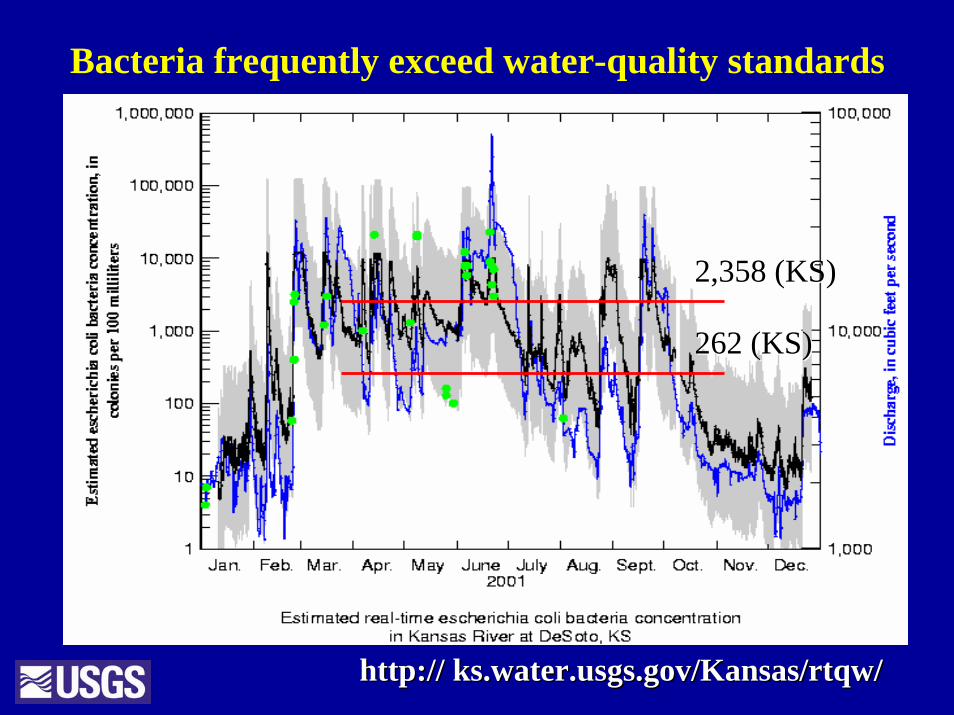
Many links to continuous waterMany links to continuous water--quality data quality data are now available compared to 5 years agoare now available compared to 5 years ago•• ks.water.usgs.gov/Kansas/rtqwks.water.usgs.gov/Kansas/rtqw//
Texas Commission on Environmental QualityTexas Commission on Environmental Qualityhttp://www.tceq.state.tx.us/compliance/monitoring/water/quality/http://www.tceq.state.tx.us/compliance/monitoring/water/quality/data/wqm/swqm_data/wqm/swqm_realtime_swf.html#datarealtime_swf.html#data
TCEQ Green CreekTCEQ Green Creek
YSI ROX YSI Extended Deployment System (EDS)
Hydrolab
LDO
Examples of comparisons of different dissolved Examples of comparisons of different dissolved oxygen (DO) and turbidity instrumentsoxygen (DO) and turbidity instruments
Clark cell/optical DO methods are similar, but not equalClark cell/optical DO methods are similar, but not equal
USGS Open-File Report 2006-1047
The murkiness of turbidity measurementThe murkiness of turbidity measurement
• Operationally defined by method used and instrument configuration using nephelometry
• “an expression of the optical properties of a sample that causes light rays to be scattered and absorbed rather than transmitted in straight lines through a sample. (Turbidity of water is caused by the presence of suspended and dissolved matter such as clay, silt, finely divided organic matter, plankton, other microscopic organisms, organic acids, and dyes)”
Are these 3 turbidities comparable/equivalent?Are these 3 turbidities comparable/equivalent?
20032003
““ NT
UN
TU
””
Sensor maxima for 6026Sensor maxima for 6026
YSI 6026, 6136, and YSI 6026, 6136, and HydrolabHydrolab ““3,0003,000”” turbidity are turbidity are comparable, but not comparable, but not ““equalequal””
Y=0.63XY=0.63XRR22=0.99=0.99
6136
6136
60266026
6136
6136
HydrolabHydrolab
Measurement Measurement method needsmethod needs
to be to be stored with datastored with data
Data must be qualityData must be quality--assuredassured
From Water Quality Monitor guidelinesFrom Water Quality Monitor guidelines--Wagner and others, 2006Wagner and others, 2006
StreamflowStreamflow relation to water quality is complex and variablerelation to water quality is complex and variable
•• 78 events (flow 78 events (flow exceeded 100 exceeded 100 cfscfs))——comprised 99 percent comprised 99 percent of the load for the 6of the load for the 6--year periodyear period
•• Largest event was 8 Largest event was 8 percent of the load for percent of the load for the 6the 6--year period and year period and occurred over 8 days occurred over 8 days (0.3 percent of time)(0.3 percent of time)
•• Only 5 events exceeded Only 5 events exceeded the 2the 2--year floodyear flood
•• Average event Average event ----6 days, 6 days, maximum maximum ----25 days25 days
Tur
bidi
ty, F
NU
Tur
bidi
ty, F
NU
StreamflowStreamflow
Continuous data is Continuous data is necessary to necessary to understand the understand the waterwater--quality quality response to response to streamflowstreamflow
Mill Creek April 28Mill Creek April 28--29, 2006 29, 2006 hysteresishysteresis
00
11 22 33
0. Q inc. within 15 min.0. Q inc. within 15 min.
1. source limit reached1. source limit reached
2. new 2. new tribtrib or bank collapseor bank collapsesourcesource
3. response to 3. response to precipprecip and and new new tribstribs
Continuous waterContinuous water--quality technology and estimates quality technology and estimates
•• RealReal--time water quality is technology driven and must stay currenttime water quality is technology driven and must stay current
•• Need to understand the measurement technology and limits Need to understand the measurement technology and limits
•• Data storage can and must be differentiatedData storage can and must be differentiated
•• New challenge is how to interpret the wealth of the timeNew challenge is how to interpret the wealth of the time--dense data dense data that challenges our assumptionsthat challenges our assumptions
Next Up Data and QA, followed by statistical estimation approachNext Up Data and QA, followed by statistical estimation approach
Any questions/comments/discussion/concerns?Any questions/comments/discussion/concerns?
RealReal--Time and Quality Assurance Time and Quality Assurance Aspects of Continuous WaterAspects of Continuous Water--Quality Quality
Monitor DataMonitor Data
Trudy BennettTrudy BennettUSGS Kansas Water Science CenterUSGS Kansas Water Science Center
QualityQuality--assurance of realassurance of real--time watertime water--quality monitor dataquality monitor data
•• GOAL is to optimize retained data of GOAL is to optimize retained data of known quality known quality •• Identify transmission problemsIdentify transmission problems•• Recognize erroneous data due to Recognize erroneous data due to
fouling or calibration driftfouling or calibration drift•• Recognize erroneous data due to Recognize erroneous data due to
sensor or monitor malfunctionsensor or monitor malfunction
Transmission ProblemsTransmission Problems
Turbidity Sensor Buried in SandTurbidity Sensor Buried in Sand
Retained turbidity data
Discharge
Turbidity dataproblems
DO Sensor Calibration FailureDO Sensor Calibration Failure
Turbidity Sensor FailureTurbidity Sensor Failure
QA/QC of Web DataQA/QC of Web Data
•• GOAL is to Optimize Accuracy of Data GOAL is to Optimize Accuracy of Data Viewed on WebViewed on Web•• Delete erroneous dataDelete erroneous data•• Resolve data problemsResolve data problems•• Apply corrections to update data for Apply corrections to update data for
fouling and/or calibration driftfouling and/or calibration drift•• Update WebUpdate Web
QA/QC Critical Steps of Transmitted QA/QC Critical Steps of Transmitted DataData
1.1. Daily Office Review of Transmitted DataDaily Office Review of Transmitted Data2.2. Field Work ProtocolsField Work Protocols3.3. Record Working ProcessRecord Working Process
1.1. Daily Review of Transmitted DataDaily Review of Transmitted Data2.2. Delete Erroneous DataDelete Erroneous Data3.3. Set Thresholds (recommended)Set Thresholds (recommended)4.4. Remove Site or Parameter from Web Remove Site or Parameter from Web
(last option)(last option)
Zero Values Caused when Monitor was Zero Values Caused when Monitor was ServicedServiced
Sensor Noise in Conductivity SensorSensor Noise in Conductivity Sensor
Sensor Noise (cont.)Sensor Noise (cont.)
Step 1. Office Work (cont.)Step 1. Office Work (cont.)
1.1. Daily Review of Transmitted DataDaily Review of Transmitted Data2.2. Delete Erroneous DataDelete Erroneous Data3.3. Set Thresholds (recommended)Set Thresholds (recommended)4.4. Remove Site or Parameter from Web Remove Site or Parameter from Web
(last option)(last option)
Spike in Transmitted DataSpike in Transmitted Data
Step 1. Office Work (cont.)Step 1. Office Work (cont.)
1.1. Daily Review of Transmitted DataDaily Review of Transmitted Data2.2. Delete Erroneous DataDelete Erroneous Data3.3. Set Thresholds (recommended)Set Thresholds (recommended)4.4. Remove Site or Parameter from Web Remove Site or Parameter from Web
(last option)(last option)
USGS Program for Setting Thresholds USGS Program for Setting Thresholds LimitsLimits
Thresholds are Site SpecificThresholds are Site Specific(example)(example)
Spike in Transmitted DataSpike in Transmitted Data
Thresholds Effect on NWIS WebThresholds Effect on NWIS Web
Caution in Setting Thresholds LimitsCaution in Setting Thresholds Limits
Thresholds Settings May Need to be Thresholds Settings May Need to be AdjustedAdjusted
Plot Data with Other ParametersPlot Data with Other Parameters
SC
Turbidity
Discharge
NWIS Web after Resetting ThresholdsNWIS Web after Resetting Thresholds
Step 1. Office Work (cont.)Step 1. Office Work (cont.)
1.1. Daily ReviewDaily Review2.2. Delete Invalid DataDelete Invalid Data3.3. Set Thresholds (recommended)Set Thresholds (recommended)4.4. Temporarily Remove Site or Parameter Temporarily Remove Site or Parameter
from Web until problem is fixed (last from Web until problem is fixed (last option)option)
Step 2. Field Work ProtocolsStep 2. Field Work Protocols
Standard Protocols for Servicing a MonitorStandard Protocols for Servicing a Monitor1.1. Before cleaning readings Before cleaning readings ******2.2. After cleaning readings After cleaning readings ******3.3. Calibration checksCalibration checks4.4. ReRe--calibration if necessarycalibration if necessary5.5. Final readings Final readings ******6.6. *** Obtain side*** Obtain side--byby--side readings side readings
from field monitor ***from field monitor ***
Step 2. Field Work ProtocolsStep 2. Field Work Protocols
Protocols were developed toProtocols were developed toDEFINEDEFINE
andandQUANTIFYQUANTIFY
why data changed after servicing the why data changed after servicing the waterwater--quality monitor and to quality monitor and to
Reasons for data to changeReasons for data to change
1.1. Cleaned the sensorsCleaned the sensors2.2. Recalibration of sensorsRecalibration of sensors3.3. Normal environmental changesNormal environmental changes
Fouling on PVC PipeFouling on PVC Pipe
Fouling on MonitorFouling on Monitor
Fouling on SensorsFouling on Sensors
Calibration ChecksCalibration Checks
USGS Calibration Criteria for USGS Calibration Criteria for Recalibrating SensorsRecalibrating Sensors
SensorSensor Variability of SensorsVariability of Sensors
Water TemperatureWater Temperature +/+/-- 0.2 0.2 ººCC
Specific ConductanceSpecific Conductance greater of +/greater of +/-- 5 5 µµS/cm or +/S/cm or +/-- 3% 3%
1.1. Determined by step 3 of field work Determined by step 3 of field work protocols.protocols.
2.2. Standard value Standard value –– Sensor reading in std.Sensor reading in std.3.3. % value: [(Std % value: [(Std –– Reading) / Reading].Reading) / Reading].
Computed DO Drift CorrectionComputed DO Drift Correctionusing developed spreadsheetsusing developed spreadsheets
DO Data After Applying a DO Data After Applying a --10% Drift 10% Drift CorrectionCorrection
Raw DataRaw DataComputed Data with Computed Data with --10% correction10% correction
USGS Maximum Allowable Limits for USGS Maximum Allowable Limits for Reporting DataReporting Data
ParameterParameter Maximum LimitMaximum LimitWater TemperatureWater Temperature +/+/-- 2.0 2.0 ººC C
Specific ConductanceSpecific Conductance +/+/-- 30% 30% µµS/cmS/cm
pHpH +/+/-- 2.0 pH unit 2.0 pH unit
Dissolved OxygenDissolved Oxygen Greater of +/Greater of +/-- 2.0 mg/L or +/2.0 mg/L or +/-- 20% 20%
TurbidityTurbidity Greater of 3.0 turbidity units or Greater of 3.0 turbidity units or +/+/-- 30%30%
Summary of QA/QC of RealSummary of QA/QC of Real--Time Time WaterWater--Quality Monitor RecordsQuality Monitor Records
1.1. Daily Review of Transmitted DataDaily Review of Transmitted Data2.2. Delete Erroneous DataDelete Erroneous Data3.3. Follow Standard Protocols for Servicing Follow Standard Protocols for Servicing
the Monitorthe Monitor4.4. Apply Corrections to Update DataApply Corrections to Update Data5.5. Update Data on Web (if transmitting)Update Data on Web (if transmitting)
For Additional InformationFor Additional Information
Statistical Approaches and Data Statistical Approaches and Data Applications for Continuous Applications for Continuous WaterWater--Quality InformationQuality Information
Teresa Rasmussen, Teresa Rasmussen,
USGS Kansas Water Science USGS Kansas Water Science CenterCenter
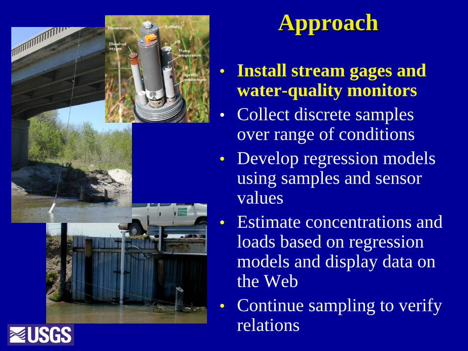
ApproachApproach
• Install stream gages and water-quality monitors
• Collect discrete samples over range of conditions
• Develop regression models using samples and sensor values
• Estimate concentrations and loads based on regression models and display data on the Web
• Continue sampling to verify relations
Kansas River at DeSoto, 1999-2002
Is monitor location representative of stream crossIs monitor location representative of stream cross--section?section?
Average cross-section turbidity, FNUs
Turb
idity
(in
-str
eam
mon
itor)
, FN
Us
Approach Approach
• Install stream gages and water-quality monitors
• Collect discrete samples over range of conditions
• Develop regression models using samples and sensor values
• Estimate concentrations and loads based on regression models and display data on the Web
Edwards and Edwards and GlyssonGlysson, 1998, 1998
3. Autosampler3. Autosampler
Collect samples over Collect samples over
the range of conditionsthe range of conditions
Kansas River at DeSoto, 1999Kansas River at DeSoto, 1999--20032003
Duration curves for Duration curves for streamflowstreamflow, turbidity, and , turbidity, and
specific conductancespecific conductance
Approach • Install stream gages and
water-quality monitors• Collect discrete samples
over range of conditions • Develop regression models
using samples and sensor values
• Estimate concentrations and loads based on regression models and display data on the Web
• Continue sampling to verify relations
log ECB = 1.66logTBY – 0.362 R2 = .86
log SSC = 1.14logTBY – 0.050 R2 = .98
Estim
ated
Estim
ated
Estim
ated
Estim
ated
MeasuredMeasured
MeasuredMeasured
Plot the dataPlot the data
What variables What variables should be included?should be included?PRESS (Prediction Error Sum of PRESS (Prediction Error Sum of Squares) Squares) –– measure of goodness of fitmeasure of goodness of fit
MallowMallow’’s Cp s Cp –– minimize bias and variance minimize bias and variance associated with multiple coefficientsassociated with multiple coefficients
Evaluate modelsEvaluate modelsResiduals vs fit
Response vs fit
Select the Select the ‘‘bestbest’’ modelmodel
Other factors to consider in model developmentOther factors to consider in model development
•• Should data be transformed? If so, apply a bias Should data be transformed? If so, apply a bias correction factor?correction factor?
•• Outliers Outliers –– how to define and what to do with them?how to define and what to do with them?
•• Estimate missing data?Estimate missing data?
•• Site specific models or combine sites?Site specific models or combine sites?
•• How many samples are needed? Over what period How many samples are needed? Over what period of time are they collected?of time are they collected?
•• Changes in sensor technologyChanges in sensor technology
ReRe--evaluate the final modelsevaluate the final models
Rasmussen, Ziegler, and Rasmussen 2005
Procedures for developing a regression modelProcedures for developing a regression model
•• Plot the dataPlot the data•• Determine which variables to includeDetermine which variables to include•• Should the variables be transformed?Should the variables be transformed?•• Graphically evaluate Graphically evaluate
homoscedasticity, normality of homoscedasticity, normality of residuals, and curvature in residuals residuals, and curvature in residuals vs. predicted.vs. predicted.
•• Select the simplest model that best Select the simplest model that best maximizes Rmaximizes R2 2 and minimizes PRESSand minimizes PRESS
•• Evaluate the model in terms of Evaluate the model in terms of physical basis, statistics, prediction physical basis, statistics, prediction intervals, probability distributionsintervals, probability distributions
TurbidityTurbidity Total suspended solids, Total suspended solids, suspended sediment, suspended sediment, fecal coliform, E. coli, fecal coliform, E. coli, total nitrogen, total total nitrogen, total phosphorus, phosphorus, geosmingeosmin
ConstituentConstituent ModelModel RR22 MSEMSE
Total nitrogenTotal nitrogen 0.7960.796 0.02260.0226
Total organic nitrogenTotal organic nitrogen 0.8170.817 0.33000.3300
Total phosphorusTotal phosphorus 0.9280.928 0.01480.0148
over range of conditions • Develop regression models
using samples and sensor values
• Estimate concentrations and loads based on regression models and display data on the Web
• Continue sampling to verify relations
Applications and examplesApplications and examples•• Time series dataTime series data•• Scatter plotsScatter plots•• Duration curvesDuration curves•• ComparisonsComparisons•• WQ criteriaWQ criteria•• TMDLsTMDLs
WaterWater--quality varies hourly, daily, quality varies hourly, daily, monthly, seasonally, and annuallymonthly, seasonally, and annually
Turb
idity
, FN
U; S
C, µ
s/cm
Stre
amflo
w, c
fs
DO
, mg/
L; p
H, p
H u
nits
Rasmussen, Ziegler, and Rasmussen 2005
Turbidity and streamflow not directly relatedTurbidity and streamflow not directly related
During 2000During 2000--03 03 E.Coli E.Coli bacteria density at Topeka exceeded bacteria density at Topeka exceeded the primary contact criterion 40% of the time.the primary contact criterion 40% of the time.
Rasmussen, Ziegler, and Rasmussen 2005
E.C
oli b
acte
ria, c
ol/1
00m
LE.Coli density generally largest at Topeka
E.C
oli b
acte
ria, c
ol/1
00 m
L
During the spring, the primary contact criterion was exceeded 80% of the time and the secondary contact criterion was exceeded 25% of the time.
Rasmussen, Ziegler, and Rasmussen 2005
90 percent of the load occurs in 7 percent of the time90 percent of the load occurs in 7 percent of the time
Little Arkansas River nr. Halstead Little Arkansas River nr. Halstead 19991999--20042004
Percentage of time load is equaled or exceededPercentage of time load is equaled or exceeded
Perc
enta
ge o
f loa
d fr
om 1
999
Perc
enta
ge o
f loa
d fr
om 1
999 --
2004
2004
Turbidity, FNU, YSI 6026 sensor
Turbidity to estimate probability of exceeding E. coli criteriaTurbidity to estimate probability of exceeding E. coli criteriaPr
obab
ility
of e
xcee
danc
e, p
erce
nt
Rasmussen and Ziegler, 2003
• Establishes range of conditions when criterion is likely to be exceeded - when turbidity is greater than 350 FNUs.• Establishes TMDL goals that incorporate continuous data -less than 10% of estimated geometric means are to exceed primary criterion and exceedences occur at flows exceeded less than 20% of the time.
Kansas River TMDL incorporates continuous turbidity data.Kansas River TMDL incorporates continuous turbidity data.When turbidity > 350 FNU, When turbidity > 350 FNU, E. coliE. coli criteria likely to be exceeded.criteria likely to be exceeded.
(Figure from KDHE, E.Coli Bacteria TMDL for Kansas-Lower Republican Basin, 2005)
•• Geosmin was detected in a near shore Geosmin was detected in a near shore surface accumulation of cyanobacteria, but surface accumulation of cyanobacteria, but not in open water samplesnot in open water samples
•• The model predicted the elevated geosmin The model predicted the elevated geosmin levels that occurred in the surface levels that occurred in the surface accumulation of cyanobacteria; had the accumulation of cyanobacteria; had the accumulation not been sampled, the model accumulation not been sampled, the model would have appeared to give an incorrect would have appeared to give an incorrect estimation of geosmin concentrationestimation of geosmin concentration
•• Spatial (both vertical and horizontal) Spatial (both vertical and horizontal) changes in the distribution of changes in the distribution of cyanobacteria may substantially influence cyanobacteria may substantially influence the occurrence of taste and odor episodesthe occurrence of taste and odor episodes
Future: RealFuture: Real--time estimation of time estimation of geosmingeosmin in Cheney Reservoir (2005)in Cheney Reservoir (2005)
Continuous monitoring and developing relationsContinuous monitoring and developing relations•• Purchase or rent monitor and installPurchase or rent monitor and install•• O&M for 6 sensors and records O&M for 6 sensors and records •• Sampling (15Sampling (15--30 times over 2 years)30 times over 2 years)•• Regression analysis and report Regression analysis and report •• Put estimates on the webPut estimates on the web
Subsequent yearsSubsequent years•• O&M for 6 sensors and recordsO&M for 6 sensors and records•• Sampling (3Sampling (3--5 times per year)5 times per year)
Benefits of Real Time Water Quality• Improve our understanding of the hydrology and
water quality of streams• Continuously measure water quality in real time
like streamflow• Comparison to water-quality criteria• Provide notification of changes in water-quality
conditions for water treatment and recreation in real time
• Better estimate selected constituent concentrations and loads with defined uncertainty
• Identify source areas and evaluate trends for NPDES, BMPs and TMDLs
• Optimize timing of sample collection
Future Challenges for Continuous Water QualityFuture Challenges for Continuous Water Quality•• Need more and better direct measurement sensorsNeed more and better direct measurement sensors•• Reduce O&M costs/timeReduce O&M costs/time•• Ice and shallow water installations Ice and shallow water installations •• More installations nationwide to better understand More installations nationwide to better understand
variability variability •• Detection of waterDetection of water--quality trends and quality trends and BMPsBMPs
effectivenesseffectiveness•• Improve ways to estimate and communicate Improve ways to estimate and communicate
uncertaintyuncertainty•• Continued sampling to document that relations Continued sampling to document that relations
remain representativeremain representative
http://http://ks.water.usgs.gov/Kansas/rtqwks.water.usgs.gov/Kansas/rtqw//Real-time continuous concentrations and loads on the Web—
Grain sizes and turbidity measurementGrain sizes and turbidity measurement
From From VanousVanous, Larson, and , Larson, and HachHach, Water Analysis Volume 1, 1982, Academic Press, Inc, Water Analysis Volume 1, 1982, Academic Press, Inc
1 um1 um
Scattering of light by substances in waterScattering of light by substances in water
From Brumberger and other “Light Scattering”Science and Technology, 1968Reproduced from Sadar, 1998
ISO
702
7G
LI M
etho
d 2
860 EPA 180.1
Turbidity schematicTurbidity schematic
From Mike Sadar, Turbidity Instrument Comparison HACH, 1999Technical Information Series, 7063
Color can affect turbidityColor can affect turbidityPowder activated carbonPowder activated carbon Kansas soilKansas soil Powdered limestonePowdered limestone
••Q explains only about 70 percent of the variabilityQ explains only about 70 percent of the variability••Little change in relation in 40 yearsLittle change in relation in 40 years
StreamflowStreamflow, in cubic feet per second , in cubic feet per second
Susp
ende
dSu
spen
ded --
sedi
men
t con
cent
ratio
n, in
se
dim
ent c
once
ntra
tion,
in
mill
igra
ms p
er li
ter
m
illig
ram
s per
lite
r
(Albert and Strammel, 1966)
How can changes be documented with factor of 10 variability in How can changes be documented with factor of 10 variability in concentration and concentration and streamflowstreamflow for the equivalent load?for the equivalent load?
•• Capture the variability during the largest Capture the variability during the largest streamflowsstreamflows•• Compare the storm yieldsCompare the storm yields
2-yr flood
5-yr flood
10-yr flood
Little Arkansas River nr. Halstead, KansasLittle Arkansas River nr. Halstead, Kansas
Sediment loadSediment load
Sediment concentrationSediment concentration
StreamflowStreamflow
Annual loads and yields unchanged in last 40 yearsAnnual loads and yields unchanged in last 40 years
YieldYield
Load Load
Turbidity provides an accurate estimate Turbidity provides an accurate estimate of suspendedof suspended--sediment concentrationssediment concentrations
Susp
ende
dSu
spen
ded --
sedi
men
t con
cent
ratio
n, in
se
dim
ent c
once
ntra
tion,
in
mill
igra
ms p
er li
ter
m
illig
ram
s per
lite
r
Turbidity, in Turbidity, in formazinformazin nephelometricnephelometric units, YSI 6026 sensorunits, YSI 6026 sensor
Feca
l col
iform
bac
teria
Estimated bacteria using 30Estimated bacteria using 30--day geometric meanday geometric mean


![PERFORMANCE ERIFICATION TATEMENT For Hach ......Ref. No. [UMCES] CBL 2016-014 ACT VS16-05 1 PERFORMANCE VERIFICATION STATEMENT For Hach Hydrolab DS5X and HL4 Dissolved Oxygen Sensors](https://static.documents.pub/doc/80x56/5f84f628de9cbc34626d741a/performance-erification-tatement-for-hach-ref-no-umces-cbl-2016-014.jpg)
