REAL TIME EDGE DETECTION USING SUNDANCE VIDEO AND...

REAL TIME EDGE DETECTION USING SUNDANCE

VIDEO AND IMAGE PROCESSING SYSTEM

A THESIS SUBMITTED IN PARTIAL FULFILLMENT OF THE

REQUIREMENTS FOR THE DEGREE OF

Master of Technology

In

VLSI Design and Embedded System

By

Rajeev Kanwar

Roll No: 207EC212

Department of Electronics and Communication

Engineering

National Institute of Technology

Rourkela

2007-2009

REAL TIME EDGE DETECTION USING SUNDANCE

VIDEO AND IMAGE PROCESSING SYSTEM

A THESIS SUBMITTED IN PARTIAL FULFILLMENT OF THE

REQUIREMENTS FOR THE DEGREE OF

Master of Technology

In

VLSI Design and Embedded System

By

Rajeev Kanwar

Roll No: 207EC212

Under the Guidance of

Asst. Prof. Dr. S.MEHER

Department of Electronics and Communication Engineering


Rourkela

2007-2009


Rourkela

CERTIFICATE

This is to certify that the thesis titled. “Real-Time Edge Detection Using Sundance

Video and Image Processing System” submitted by Mr. Rajeev Kanwar in partial

fulfillment of the requirements for the award of Master of Technology Degree in Electronics

and Communication Engineering with specialization in “VLSI Design And Embedded

System” at the National Institute of Technology, Rourkela (Deemed University) is an

authentic work carried out by him under my supervision and guidance.

To the best of my knowledge, the matter embodied in the thesis has not been

submitted to any other University/Institute for the award of any Degree or Diploma.

Date: 25th May, 2009 Dr. S.MEHER

Asst. Professor

Dept. of Electronics and Communication Engg.


Rourkela-769 008

ACKNOWLEDGEMENTS

This project is by far the most significant accomplishment in my life and it would be

impossible without people who supported me and believed in me.

I would like to extend my gratitude and my sincere thanks to my honorable, esteemed

supervisor Prof. S. Meher, Department of Electronics and Communication Engineering. He is not

only a great lecturer with deep vision but also and most importantly a kind person. I sincerely thank

for his exemplary guidance and encouragement. His trust and support inspired me in the most

important moments of making right decisions and I am glad to work with him.

I want to thank all my teachers Prof. G.S. Rath, Prof. G.Panda, Prof. K. K. Mahapatra, Prof.

S.K. Patra and for providing a solid background for my studies and research thereafter. They have

been great sources of inspiration to me and I thank them from the bottom of my heart.

I would like to thank all my friends and especially my classmates for all the thoughtful and

mind stimulating discussions we had, which prompted us to think beyond the obvious. I’ve enjoyed

their companionship so much during my stay at NIT, Rourkela.

I would like to thank all those who made my stay in Rourkela an unforgettable and

rewarding experience.

Last but not least I would like to thank my parents, who taught me the value of hard work

by their own example. They rendered me enormous support during the whole tenure of my stay in

NIT Rourkela.

RAJEEV KANWAR

CONTENTS

Page no.

Abstract i

List of Figure ii

List of Table iii

CHAPTER 1 Introduction 1-10

1.1 Introduction 2

1.2 Literature Review 3

CHAPTER 2 Hardware of Sundance Modules SMT339 11-27

2.1 Introduction 12

2.2 Functional Description 13

2.2.1 Block Diagram 13

2.2.2 Data Flow 14

2.3 Memory Map 16

2.3.1DSP memory map 16

2.3.2 VIRTEX 4 memory map 16

2.4 DSP Unit 16

2.4.1 EMIF peripheral configuration 17

2.4.2 I2C control 17

2.4.3 Flash 18

2.4.4 SDRAM 18

2.5 VERTEX 4 FPGA 18

2.5.1 VIRTEX 4 peripherals 19

2.5.2 LED register 19

2.5.3 Comports 19

2.6 Video Encoder and Decoder 20

2.6.1 Video Encoder/Decoder 20

2.6.2 Video encoder register 20

2.6.3 Video Decoder register 21

2.7 High Speed Nt (ZBT) Memory 22

2.8 SLB Interface 22

2.9 Video Ports Others Module 23

2.9.1 Video encoder setup 23

2.9.2 Video Memory 24

2.9.3 EDMA 24

2.9.4 RGB656 single bank EDMA setup 24

2.9.5 RGB656 with embedded sync EDMA setup 25

2.9.6 JTAG 25

2.9.7 Cabels and connectors 25

2.10 Power Consumptions 26

2.11 The Software Supporting Role 26

CHAPTER 3 Edge Detection Techniques Using Sundance Module 28-61

3.1 Introduction to Fundamentals of Edge Detection 29

3.2 A Simple Edge Model 32

3.3 Edge Detection 33

3.4 The Four Step of Edge Detection 35

3.5 Edge Detection Using Derivatives 36

3.6 Edge Detection Using Gradient 38

3.6.1 Definition of the gradient 38

3.6.2 Properties of the gradient 39

3.6.3 Estimating the gradient with finite differences 39

3.7 Different Type of Edge Detector 40

3.7.1 Sobel edge detector 41

3.7.2 Prewitt Edge Detector 46

3.7.3 Canny Edge Detector 48

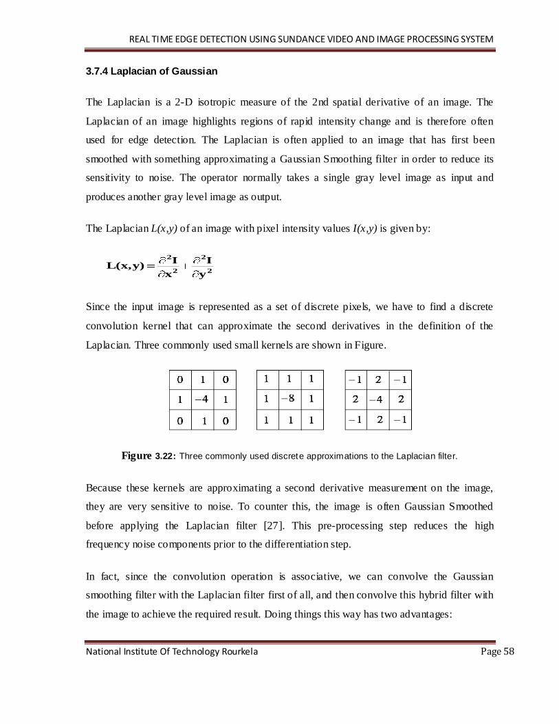
3.7.4 Laplacian of Gaussian 58

CHAPTER 4 Result and Discussions 62-66

4.1 Result of the different operator 63

4.2 comparison and discussion 65

CHAPTER 5 Conclusions and scope of Future work 67-69

6.1 Conclusion 68

6.2 Future Work 68

References 70

LIST OF FIGURE

Figure No. Figure Title Page No.

Figure 2.1 Block Diagram for SMT339 13

Figure 2.2 Data flow diagram 14

Figure2.3 Flow from Video Memory to Encoder 23

Figure 2.4 Video Memory organisation in YCbCr output mode 24

Figure2.5 RGB565 organisation of the video memory 24

Figure3.1 Following signal apply to the edge detector 30

Figure3.2 The gradient first derivative signal 30

Figure3.3 The gradient second derivative signal 31

Figure3.4 Example of different types of edges 32

Figure3.5 Edge Detection Using Derivatives 36

Figure3.6 The edge direction is rotated with respect to the gradient direction 39

by -90 degrees

Figure3.7 Sobel convolution kernels 40

Figure3.8 Pseudo-convolution kernels used to quickly compute approximate 41

gradient magnitude

Figure3.9 Sobel Explanation how to get output b22 42

Figure3.10 Proposed architecture for sobel edge detection operator. 44

Figure3.11 Masks for the Prewitt gradient edge detector. 46

Figure3.12 Result of Sobel and Prewitt Operator 47

Figure3.13 Discrete Approximation to Gaussian function with σ=1.4 49

Figure3.14 The Sobel operator uses a pair of 3x3 convolution mas 49

Figure3.15 The Orientation Angle is Found to be 3 Degrees 51

Figure3.16 Block diagram implementation of Canny algorithm 53

Figure3.17 Hardware Implementation of non-symmetric 2D filter 54

Figure 3.18: Hardware implementation of symmetric separable 2D filter 55

Figure 3.19: Determine orientation of gradient in the nonmaximal suppression 55

stage

Figure 3.20: Edge strength classification map 56

Figure 3.21: Result of Canny Operator 57

Figure 3.22: Three commonly used discrete approximations to the Laplacian 58

filter.

Figure 3.23: The 2-D Laplacian of Gaussian (LoG) function. The x and y axes 59

are marked in standard deviations (σ)

Figure 3.24: Discrete approximation to LoG function with Gaussian σ = 1.4 59

Figure 3.25: Response of 1-D LoG filter to a step edge 60

Figure 3.26: Result of Laplacian operator 61

Figure 4.1: Result of the all the operator 63

LIST OF TABLES

Table No. Table Title Page No.

Table 2.1 DSP Memory Map Description 16

Table 2.2 Virtex 4 Internal Peripherals Memory Map Description 16

Table 2.3 EMIF Configurations. 17

Table 2.4 I2C CONTROL 17

Table 2.5 Shows the GPIO pins values and associated memory access areas. 18

Table 2.6 Virtex 4 LED Register bit Definitions 19

Table 2.7 Virtex 4, Video Encoder Register 20

Table 2.8 Virtex 4, Video Decoder Register 21

Table 2.9 Video Port 0 and Decoder connectivity 21

Table 2.10 Video Port 0 and Decoder Clock connectivity 22

Table 2.11 Video Port 0 Decoder Data to Video Port Data Mapping 22

Table 2.12 JP5 Virtex JTAG Header 25

Table 2.13 JP7 Connector 26

Table 3.1 shows the implementation complexity of the different class of filters 54

as a function of number of multiplication operations

ABSTRACT

Edge detection from images is one of the most important concerns in digital image and

video processing. With development in technology, edge detection has been greatly

benefited and new avenues for research opened up, one such field being the real time video

and image processing whose applications have allowed other digital image and video

processing. It consists of the implementation of various image processing algorithms like

edge detection using sobel, prewitt, canny and laplacian etc. A different technique is

reported to increase the performance of the edge detection. The algorithmic computations in

real-time may have high level of time based complexity and hence the use of Sundance

Module Video and Image processing system for the implementation of such algorithms is

proposed here. In this module is based on the Sundance module SMT339 processor is a

dedicated high speed image processing module for use in a wide range of image analysis

systems. This processor is combination of the DSP and FPGA processor. The image

processing engine is based upon the „Texas Instruments‟ TMS320DM642 Video Digital

Signal Processor. And A powerful Vitrex-4 FPGA (XC4VFX60-10) is used onboard as the

FPGA processing unit for image data. It is observed that techniques which follow the stage

process of detection of noise and filtering of noisy pixels achieve better performance than

others. In this thesis such schemes of sobel, prewitt, canny and laplacian detector are

proposed.

Chapter 1

Introduction

REAL TIME EDGE DETECTION USING SUNDANCE VIDEO AND IMAGE PROCESSING SYSTEM

National Institute Of Technology Rourkela Page 2

1.1 INTRODUCTION

Digital image processing is an ever expanding and dynamic area with applications reaching

out into our everyday life such as in medicine, space exploration, surveillance,

authentication, automated industry inspection and in many more areas.

Applications such as these involve different processes like image enhancement, and object

detection. Implementing such applications on a generable purpose computer can be easier

but not very efficient in terms of speed. The reason being the additional constraints put on

memory and other peripheral device management. Application specific hardware offers

much greater speed than a software implementation.

There are two types of technologies available for hardware design. Full custom hardware

design also called as Application Specific Integrated Circuits (ASIC) and semi custom

hardware device, which are programmable devices like Digital signal processors (DSP‟s)

and Field Programmable Gate Arrays (FPGA‟s).

Full custom ASIC design offers highest performance, but the complexity and the cost

associated with the design is very high. The ASIC design cannot be changed; time taken to

design the hardware is also very high. ASIC designs are used in high volume commercial

applications. In addition, if an error exist in the hardware design, once the design is

fabricated, the product goes useless.

DSP‟s are a class of hardware devices that fall somewhere between an ASIC and a PC in

terms of the performance and the design complexity. DSP‟s are specialized microprocessor,

typically programmed in C, perhaps with assembly code for performance. It is well suited to

extremely complex math intensive tasks such as image processing. Hardware design

knowledge is still required, but the learning curve is much lower than some other design

choices.

Field Programmable Gate Arrays are programmable devices. They are also called

reconfigurable devices. Reconfigurable devices are processors which can be programmed

with a design, and the design can be by reprogramming the devices. Hardware design

techniques such as parallelism and pipelining techniques can be developed on a FPGA,



which is not possible in dedicated DSP designs. So FPGAs are ideal choice for

implementation of real time image processing algorithms.

FPGAs have traditionally been configured by hardware engineers using a Hardware Design

Language (HDL). The principal languages being used are VHDL.VHDL are specialized

design techniques that are not immediately accessible to software engineers, who have often

been trained using imperative programming languages. Consequently, over the last few

years there have been several attempts at translating algorithmic oriented programming

languages directly into hardware descriptions. The combination of FPGA AND DSP

processors description language by Sundance module SMT339, allows the designer to focus

more on the specification of an algorithm rather than adopting a structural approach to

coding. For these reasons the used for implementation of image processing algorithms on

FPGA. The SMT339 provides video input and video output using the TMS320DM642 from

Texas Instruments. The hardware is extremely flexible but that comes at the price of

enormous complexity. It can take a long time to determine values for all the relevant

registers of the numerous components in the processor; a slight error can result in bizarre

effects ranging from no input or output at all to strangely corrupted images.

The goal of this thesis is to implement image processing algorithms like convolution and

different edge detectors like a Sobel, Prewitt, Canny and Laplacian edge detection through

Sundance module and compare against the performance of different detector.

Chapter two provides information on the hardware Sundance module SMT339 and prior

related work. Chapter three describes the edge detection algorithms. Chapter four provides

the result and discussion. Chapter five summaries the results and future work.

1.2 LITRATURE REVIEW

In this section, work done in the area of edge detection is reviewed and focus has

been made on detecting the edges of the digital images. Edge detection is a problem of

fundamental importance in image analysis. In typical images, edges characterize object

boundaries and are therefore useful for segmentation, registration, and identification of

objects in a scene. Edge detection of an image reduces significantly the amount of data and



filters out information that may be regarded as less relevant, preserving the important

structural properties of an image.

A theory of edge detection is presented. The analysis proceeds in two parts.

(1)Intensity changes, which occur in a natural image over a wide range of scales, are

detected separately at different scales. An appropriate filter for this purpose at a given scale

is found to be the second derivative of a Gaussian, and provided some simple conditions are

satisfied, these primary filters need not be orientation-dependent. Thus, intensity changes at

a given scale are best detected by finding the zero values of for image. The intensity changes

thus discovered in each of the channels are then represented by oriented primitives called

zero-crossing segments. (2) Intensity changes in images arise from surface discontinuities or

from reflectance or illumination boundaries, and these all have the property that they are

spatially localized. Because of this, the zero-crossing segments from the different channels

are not independent, and rules are deduced for combining them into a description of the

image. This description is called the raw primal sketch. The theory explains several basic

psychophysical findings, and the operation of forming oriented zero-crossing segments from

the output of centre-surround filters acting on the image forms the basis for a physiological

model of simple cells.

Due to the large amount of literature on edge detection, I do not intend this to be a

comprehensive literature survey. However, in the following paragraphs, mention some

important works on edge detection and compare results to these methods. Unlike all the

other methods have encountered, the step expansion filter is based on template matching,

and specifically on the novel method of matching using non orthogonal expansion. The step

expansion filter is optimal in the sense of SNR, since Expansion Matching in general is an

optimal SNR template matching method. Other methods follow the approach of defining a

specific set of criteria for the given edge model, and optimizing them, in most cases using

numerical methods. In contrast, the Expansion Matching approach is analytical, and is

generalized so that it easily yields the optimal SNR operator for any desired edge model.

Many works have been performed on obtaining an edge detection operator. Most

noted amongst these is the work of Canny [1] who showed that the ideal operator that



maximizes the conventional signal-to-noise ratio in detecting a particular edge is correlation

with the same edge model itself. However, this detection is not well localized and requires

an additional localization criterion. A third criterion that suppresses multiple responses was

also included and numerical optimization resulted in the desired edge detector. Canny‟s edge

detector for step edges is well approximated by the Derivative of Gaussian mask. In

contrast, our edge detector formulation is based on the fact that SNR implicitly defines all

the desired properties of good detection and localization (sharp peak, good localization and

minimal off-center response), and thus given an edge model, the optimal SNR filter for this

model also results in a good edge detector. While Canny [1] worked with finite extent filters.

Deriche [2] used the same approach with infinite extent filters, with the objective of

obtaining an efficient recursive implementation. The resulting operator has the form of an

even, exponentially damped sinusoid and is different from our Step Expansion Filter.

Furthermore, the step expansion filter is also infinite in width, and has an efficient recursive

implementation as well.

Another work using infinite width filters is due to Sarkar and Boyer [3], [4]. In this

work, Canny‟s signal-to-noise ratio and localization criterion, along with another criterion

for spurious response are optimized using the variational approach and nonlinear constrained

optimization. A recursive approximation to these filters is also presented. A comprehensive

set of results with different values of the Multiple Response Criterion (MRC) reveals that for

some values of the MRC, the filters are somewhat similar in appearance to our Step

Expansion Filter. Spacek [5] combined all three of Canny‟s criteria into one performance

measure and simplified the differential equation that yields the optimal filter. To yield the

actual optimal filter, he fixed two of the six parameters involved and determined the

remaining four using boundary conditions. The work of Petrou and Kittler [6] extends

Spacek‟s works for ramp edges.

Shen, Castan, and Zhao [7], [8] present as an optimal operator for edge detection, an

exponential filter. Analytically, this exponential filter is equivalent to the integral of the Step

Expansion Filter that we present. Unlike Shen er al use Expansion Matching and optimize

the SNR criterion, and obtain an exact analytical relationship between the variance of the

expected input noise, and the width (decay parameter in the exponential term) of our Filter.



On the other hand, Shen and Castan [7] desire to: a) minimize the energy in the desired

filter‟s response to noise, b) minimize the energy in the derivative of the above noisy

response, and c) maximize the energy of the peak center response to the step edge. Unlike

the SNR, these criteria do not consider the off-center response of the filter to the template (in

this case the step edge model) as undesired noise. Also, their work does not address the

problem of determining an appropriate detector width for a given input noise. Our approach

also offers a general method for easily designing optimal SNR detectors for any edge model,

not only step edges, and can also easily incorporate colored noise models. Another important

point is that the edge maps generated by the two methods are not identical, since we detect

the peaks of the filter output, whereas Shen and Castan obtain the zero crossings of the

output of their exponential filter. The fundamental difference here is that while the step

expansion filter and the exponential filter are related by a simple integral equation, detecting

the peaks of the step expansion filter output in a white noise environment (as per our

analytical model) is not equivalent to detecting the zero crossings of in a white noise

environment (as Shen and Castan propose) since the noise model undergoes a change

(actually becomes more colored and low pass) due to the integration. A more detailed

discussion of this point can be found in the work of Sarkar and Boyer [3].

Modestino and Fries [9] suggest to use the Laplacian of an image in order to detect

edges. In their work they use random fields, and cast the problem as one of obtaining the

minimum mean squared error estimate of the true Laplacian of the actual input image from a

given noisy input image. This obviously results in the Wiener filter of the Laplacian as the

optimal filter. Modestino and Fries do not use this filter itself, but instead use a spatial

frequency weighted version of the Laplacian (basically a Gaussian low-pass spatial filter) to

avoid difficulties in the digital implementation of the optimum Wiener filter. Furthermore,

their work is concentrated on realizing this filter using a recursive implementation. Note that

their Wiener filter has no connection to the SNR optimization that we perform. The Wiener

restoration filter use is based on regarding the given edge model as a blurring function,

which has been shown to be an efficient and regularized implementation of the

nonorthogonal expansion for matching [10].



Other ideas in the field of edge detection include the work of Dickley er al. [11] who

obtained the spherical wave function as their ideal filter, based on the definition of an edge

as a step discontinuity between regions of uniform intensity. Another significant work is that

of Marr and Hildreth [12] who suggested the isotropic Laplacian of Gaussian mask on the

image and identified the resulting zero-crossings as the edges of the image. A numerical

method using interpolated data proposed by Haralick [13] involved locating edges as the

zerocrossings of the second directional derivative in the direction of the gradient. A surface-

fitting approach was used by Nalwa and Binford [14] wherein, at each point, the edge

detector performs a best- fit of surfaces within a localized window, i.e., least squared error

with minimal number of parameters.

A lot of the attention is focused to edge detection, being a crucial part in most of the

algorithms. Classically, the first stage of edge detection (e.g. the gradient operator, Robert

operator, the Sobel operator, the Prewitt operator) is the evaluation of derivatives of the

image intensity. Smoothing filter and surface fitting are used as regularization techniques to

make differentiation more immune to noise.

Raman Maini and J. S. Sobel [15] evaluated the performance of the Prewitt edge

detector for noisy image and demonstrated that the Prewitt edge detector works quite well

for digital image corrupted with Poisson noise whereas its performance decreases sharply

for other kind of noise.

Davis, L. S. [16] has suggested Gaussian preconvolution for this purpose. However,

all the Gaussian and Gaussian- like smoothing filters, while smoothing out the noise, also

remove genuine high frequency edge features, degrade localization and degrade the

detection of low- contrast edges. The classical operators emphasize the high frequency

components in the image and therefore act poorly in cases of moderate low SNR and/or low

spatial resolution of the imaging device. The awareness of this has lead to new approaches

in which balanced trade-offs between noise suppression, image deblurring and the ability to

resolve interfering edges, altogether resulting in operators acting like band-pass filters e.g.

Canny. Sharifi, M. et al. [17] introduces a new classification of most important and

commonly used edge detection algorithms, namely ISEF, Canny, Marr-Hildreth, Sobel,

Kirch and Laplacian. They discussed the advantages and disadvantages of these algorithms.



Shin, M.C et al. [18] presented an evaluation of edge detector performance using a

structure from motion task. They found that the Canny detector had the best test

performance and the best robustness in convergence and is one of the faster executing

detectors. It performs the best for the task of structure from motion. This conclusion is

similar to that reached by Heath et al. [20] in the context of human visual edge rating

experiment.

Rital, S. et al. [19] proposed a new algorithm of edge detection based on properties

of hyper graph theory and showed this algorithm is accurate, robust on both synthetic and

real image corrupted by noise. Li Dong Zhang and Du Yan Bi [21] presented an edge

detection algorithm that the gradient image is segmented in two orthogonal orientations and

local maxima are derived from the section curves. They showed that this algorithm can

improve the edge resolution and insensitivity to noise.

Zhao Yu-qian et al. [22] proposed a novel mathematic morphological algorithm to

detect lungs CT medical image edge. They showed that this algorithm is more efficient for

medical image denoising and edge detecting than the usually used template-based edge

detection algorithms such as Laplacian of Gaussian operator and Sobel edge detector, and

general morphological edge detection algorithm such as morphological gradient operation

and dilation residue edge detector.

Fesharaki, M.N.and Hellestrand, G.R [23] presented a new edge detection algorithm

based on a statistical approach using the student t-test. They selected a 5x5 window and

partitioned into eight different orientations in order to detect edges. One of the partitioning

matched with the direction of the edge in the image shows the highest values for the defined

statistic in that algorithm. They show that this method suppresses noise significantly with

preserving edges without a prior knowledge about the power of noise in the image.

Lim [25] defines an edge in an image as a boundary or contour at which a significant

change occurs in some physical aspect of the image. Edge detection is a method as

significant as thresholding. A survey of the differences between particular edge detectors is

presented by Schowengerdt [26]. Four different edge detector operators are examined and it

is shown that the Sobel edge detector provides very thick and sometimes very inaccurate



edges, especially when applied to noisy images. The LoG operator provides slightly better

results.

Edges can be detected in many ways such as Laplacian Roberts, Sobel and gradient

[27]. In both intensity and color, linear operators can detect edges through the use of masks

that represent the „ideal‟ edge steps in various directions. They can also detect lines and

curves in much the same way.

Traditional edge detectors were based on a rather small 3x3 neighborhood, which

only examined each pixel‟s nearest neighbor. This may work well but due to the size of the

neighborhood that is being examined, there are limitations to the accuracy of the final edge.

These local neighborhoods will only detect local discontinuities, and it is possible that this

may cause „false‟ edges to be extracted. „A more powerful approach is to use a set of first or

second difference operators based on neighborhoods having a range of sizes (e.g. increasing

by factors of 2) and combine their outputs, so that discontinuities can be detected at many

different scales‟ [28]. Usually, gradient operators, Laplacian operators, and zero-crossing

operators are used for edge detection. The gradient operators compute some quantity related

to the magnitude of the slope of the underlying image gray tone intensity surface of which

the observed image pixel values are noisy discretized samples. The Laplacian operators

compute some quantity related to the Laplacian of the underlying image gray tone intensity

surface. The zero-crossing operators determine whether or not the digital Laplacian or the

estimated second direction derivative has a zero-crossing within the pixel. There are many

ways to perform edge detection. However, the most may be grouped into three categories,

gradient (Approximations of the first derivative), Laplacian (Zero crossing detectors) and

Image approximation algorithms. Edge detectors based on gradient concept are the Roberts

[29], Prewit and Sobel [30] show the effect of these filters on the sensing images. The major

drawback of such an operator in segmentation is the fact that determining the actual location

of the edge, slope turn overs point, is difficult. A more effective operator is the Laplacian,

which uses the second derivative in determining the edge.

The design of edge detectors is work deals not with the design of an edge detector, but rather

the methodology for comparing edge detectors. The comparison was done by Abdou and



Pratt [31]. This was followed by work by Fram and Deutsch [32], Peli and Malah [33], and

more recently, Ramesh and Haralick [34]. The emphasis in this line of work has been to

characterize the edge detector based on local signal considerations. The typical quantitative

measures have been the probability of false alarms, probability of missed edges, errors of

estimation in the edge angle, localization errors, and the tolerance to distorted edges,

corners, and junctions.

The use of human judges to rate image outputs must be approached systematically.

Experiments must be designed and conducted carefully, and results must be interpreted with

the appropriate statistical tools. The use of statistical analysis in vision system performance

characterization has been rare. The only prior work in the area that we are aware of is that of

Nair et al. [35], who used statistical ranking procedures to compare neural network-based

object recognition systems. In a related work, in 1975 Fram and Deutsch [32] used human

subjects to judge the discriminability of certain synthetic edge signatures. These results were

then compared with the edge detectors available at that time. The focus was on human

versus machine performance rather than using human ratings to compare different edge

detectors.

There are numerous other works that describe edge detection techniques approaches.

However, I do not mention any here, since my work is aimed at using the edge detection

criterion to formulate an edge detector for a given edge model and compare our results to

the different edge detector.

Chapter 2

Hardware of Sundance

Modules SMT339



2.1 INTRODUCTION

The SMT339 is a dedicated high speed image processing module for use in a wide

range of image analysis systems. The module can be plugged into a standard TIM single

width slot and can be accessed by either a standard Comport, or Rocket Serial Link (RSL)

Interface.

The image processing engine is based upon the „Texas Instruments‟ TMS320DM642

[36] Video Digital Signal Processor. It is fully software compatible with C64x using Code

Composer Studio.

The DM642 [38] runs at a clock rate of 720MHz. It features two level cache based

architecture. There are 16K Bytes of level one program cache (Direct mapped), 16K Bytes

of level one data cache (2-Way Set-Associative) and 256K Bytes of level two cache that is

shared program and data space (Flexible RAM/Cache Allocation). The DM642 can perform

4, 16 x 16 Multiplies or 8, 8 x 8 Multiplies per clock cycle.

A powerful Vitrex-4 FPGA (XC4VFX60-10)[37] is used onboard as the FPGA

processing unit for image data. 8 Mbytes of ZBT SRAM is provided as a FPGA memory

resource. Processing functions such as Colour Space Conversion (CSC), Discrete Cosine

Transforms (DCT), Fast Fourier Transforms (FFT) and convolution can be implemented,

without using any of the DSP‟s resources.

If required, the Virtex 4 has 2 Power PC hardware cores that can be incorporated into

the system design. The Module features a single „Philips Semiconductors‟

SAA7109AE/108AE video decoder/encoder [37] that accept most PAL and NTSC

standards, and can output processed images in PAL/NTSC or VGA (1280x1024, or HD TV

Y/Pb/Pr) The DM642 has 128 Mbytes of high speed SDRAM (Micron

MT48LC64M32F2S5) available onboard for image processing and an 8Mbytes FLASH

device is fitted to store programs and FPGA configuration information. The module supports

a full Sundance LVDS Bus (SLB) interface for use with mezzanine cards providing the

flexibility for other image formats to be accepted and other output formats to be generated.



2.2 FUNCTIONAL DESCRIPTION

The basic block diagram of the SMT339 and its components is illustrated in Figure 1.

2.2.1 BLOCK DIAGRAM

\

Figure 2.1: Block Diagram for S MT339

The Texas Instruments Module (TIM) form-factor SMT339 is mounted on a carrier

that might be PCI, PCI-X, VME, Compact- PCI, or even stand-alone. The carrier provides a

home and power to the module and usually an interface to a host computer. A variety of

analog video formats can be connected to the system through its video decoder.

Alternatively, a range of digital video sources may be connected to the appropriate I/O

daughtercard. The input sources are routed to the FPGA, which is a 60,000-logic-cell

Xilinx® Virtex™-4 FX60 device. The data can be preprocessed here before passing to the

DSP. The FPGA has two independent 8-MB banks of ZBTRAM, which are ideal for frame

stores for the various pre- and post-processing functions performed on the FPGA. The DSP

is a Texas Instruments TMS320DM642 video digital signal processor. You can program it

using Texas Instruments‟s Code Composer Studio, which is fully software-compatible with



the C64x DSP range. Clocked at 720 MHz, it is capable of 5.76 GMACs per second and is

linked to the FPGA by three bidirectional video ports, with more ports for control and other

data. All of the illustrated interconnections are already implemented in the FPGA, leaving

you free to implement the specific functions required for your application. The DSP also

comes with 128 MB of fast SDRAM. This 64-bit-wide memory holds the image buffers for

the DSP and program/data space. There is an output from the FPGA to a video encoder so

that a live image (raw, part, or fully processed) can be displayed directly on a monitor –

which is particularly useful when developing algorithms. Digital output may be obtained

from the appropriate I/O daughtercard attached to the Sundance LVDS bus (SLB)[39]

interface or from high-speed serial links: connectivity to and from other modules is provided

by 16 Xilinx RocketIO™ channels in the form of four Sundance rocket serial links (RSLs),

giving the system significant expandability.

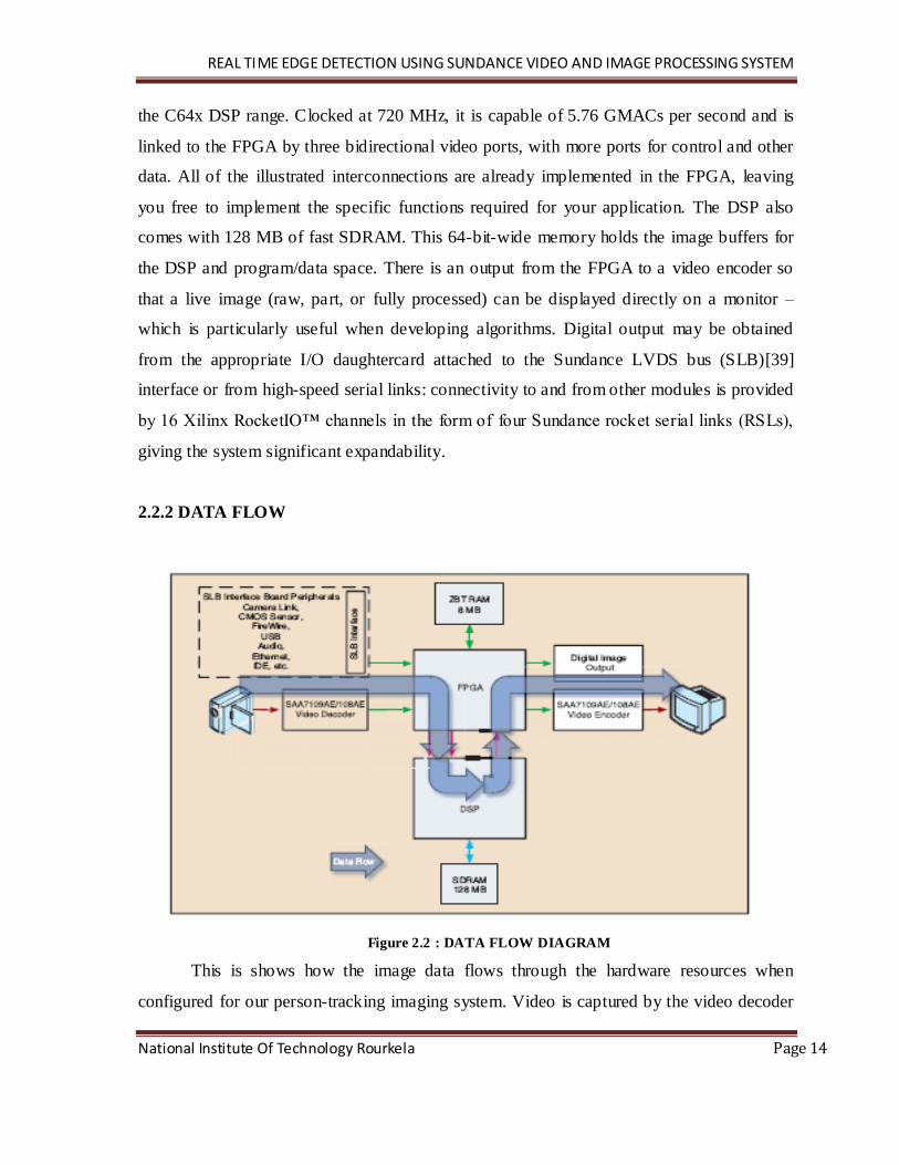
2.2.2 DATA FLOW

Figure 2.2 : DATA FLOW DIAGRAM

This is shows how the image data flows through the hardware resources when

configured for our person-tracking imaging system. Video is captured by the video decoder



and fed to the FPGA. The decoder can handle a variety of different input formats from

PAL/NTSC CVBS or separate YC. Alternatively, you can input digital video through a

daughter card digital interface module. The FPGA pre-processes the incoming video stream

using one of the ZBTRAM banks as an image buffer. A slow-moving reference image is

maintained by iterating each pixel by one bit per frame towards its value on the current

image. The current image is compared with the reference image to calculate a difference

image. A great feature of this system, with its large and powerful FPGA, is that it is very

easy to experiment with different preprocessors like spatial filters, edge enhancement filters,

or histogram functions – and see the results immediately on the system‟s live output. The

calculated difference image, together with the current image, is passed to the DSP for

analysis. The DSP performs a detection algorithm on the difference image, extracting the

silhouette and looking for the characteristic shape of a person in the moving parts of the

image.

Various properties of a person detected in the field of view can then be calculated

from this, such as:

• The coordinates of the corners of a region of interest around the person

• The center point (calculated as the mid-point of the region‟s corners)

• Their center of gravity (based on the center of the area of their silhouette)

• The coordinates of their entire outline (possibly returned in a binary overlay image of the

scene)

The FPGA then post-processes this information, recombining it with the source image. For

example, you could overlay an outline around the person, change their color, or perform

other manipulations. The results of the calculations are then available on a live video output

but they may also be output through the daughtercard or through other interfaces for transfer

to, logging, or display on digital video systems.



2.3 MEMORY MAP

The various addresses and lengths of the peripherals shown in Figure 1 are shown in Table

2.3.1 DSP MEMORY MAP

Table 2.1 DSP Memory Map Description

2.3.2 VIRTEX 4 MEMORY MAP

Table 2.2 Virtex 4 Internal Peripherals Memory Map Description

2.4 DSP UNIT

As illustrated in Figure 1 the SMT339[38] is based around the „Texas Instruments‟

TMS320DM642 Video Imaging Processor. The processor is based around the second

generation VelociTI Texas Instruments TMS320C6000 generation of processors. This

processor has 3 built- in video imaging ports (each 20 bit) which each have 2 channels

capable of sample rates up to 80MHz over a 10 bit bus, the direction of each channel being



configurable as input or output. This allows Images to be DMA‟ed directly to the SDRAM

for processing, while the processed image can be viewed on one of the output channels.

Input YCbCr formats with embedded sync information can be accepted by the video ports as

well as RAW data modes. The DM642 DSP has 128Mbytes of high speed SDRAM memory

available for program and data space, an 8Mbyte FLASH allows FPGA configuring data and

DSP program data to be stored. The DSP‟s EMIF bus is also routed to the Virtex 4 FPGA,

which allows the mapping of the Comports and the RSL directly into the DSP‟s memory

map. The EMAC, serial ports and Audio channels are routed from the DSP to the Virtex 4,

this allows the EMAC, SLB or Audio physical interfaces to be added to the system if

required. Software development and real-time debugging can be achieved using Code

Composer Studio (Texas Instruments) via the JTAG interface.

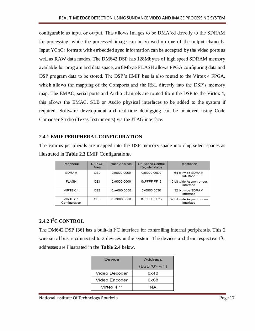
2.4.1 EMIF PERIPHERAL CONFIGURATION

The various peripherals are mapped into the DSP memory space into chip select spaces as

illustrated in Table 2.3 EMIF Configurations.

2.4.2 I2C CONTROL

The DM642 DSP [36] has a built- in I2C interface for controlling internal peripherals. This 2

wire serial bus is connected to 3 devices in the system. The devices and their respective I2C

addresses are illustrated in the Table 2.4 below.



2.4.3 FLASH

8Mbytes of flash memory is provided with direct access by the DM642. This device

contains boot code for the DSP and the configuration data for the FPGA. This is a 16-bit

wide device. The flash device can be re-programmed by the DM642 at any time. There is a

software protection mechanism to stop most errant applications from destroying the device‟s

contents. For extra safety a jumper (JP1) must be inserted to allow write operations. Note

that the flash memory is connected as a 16 bit device, but during a DM642 boot (internal

function of the C6x) only the bottom 8 bits are used. There are a number of DSP General

Purpose pins connected to the FLASH devices Bank Pins in order to allow access to the

upper FLASH areas.

Table 2.5: below shows the GPIO pins values and associated memory access areas.

2.4.4 SDRAM

There are128Mbytes of SDRAM connected to the DM642 processor via its external memory

interface (EMIF). The EMIF clock runs at 100MHz and the bus width is 64bits, organized as

2 banks of 32bits. This allows a peak data transfer rate of 400Mbytes/second.

2.5 VIRTEX 4 FPGA

The FPGA on the SMT339 is a Virtex 4 FX60 device (XC4VFX6010FF1152). It is

connected to the DSP‟s EMIF and therefore allows its internal peripherals to be accessed at

100MHz clock rates and a bus width of 64bits. This allows high speed transfers to be

initiated at request. It should, however, be noted that sustained large transfer will affect the

DSP‟s peak performance if the DSP‟s algorithm is running in external SDRAM memory. To

avoid this, the application can be run in internal DSP memory.



Some of the FPGA‟s features are listed below.

• The Virtex-4 enhanced PowerPC™ 405 core delivers 680 DMIPS performance at 450

MHz and the new Auxiliary Processor Unit (APU) controller

• 400+ MHz clock rates

• 2.8Mbits of internal block RAM available.

• Up to 444 18X18 embedded multipliers.

• Extensive library of DSP algorithms.

2.5.1 VIRTEX 4 PERIPHERALS

The Standard firmware supplied with a SMT339 contains interfaces for the peripherals listed

below.

• Mapping of 2 Video Ports and related control registers

• Mapping of 2 communication ports

• LED Register Mapping

• Video Encoder Control Register

• Video Decoder Control Register

2.5.2 LED REGISTER

There are 4 LEDS mapped in the Virtex 4 firmware that can be accessed via the DSP over

the EMIF. The resister is located at 0xA00D0000 and is mapped as follows.

Table 2.6: Virtex 4 LED Register bit Definitions

Virtex 4 LED Register bit Definitions

2.5.3 COMPORTS

There are 2 Comports implemented in the standard FPGA configuration file. Comport 3 and

Comport 2. Comport 3 is usually routed via the carrier module to the Host CPU for setup

and control by 3L or other applications. See the SMT6400 for detailed operation of how

they can be used.



2.6 VIDEO ENCODER AND DECODER

2.6.1 VIDEO ENCODER / DECODER

The encoder/decoder is based on the „Philips Semiconductors‟ SAA7109AE/108AE. This

provides decoding of PAL, NTSC and SECAM signal standards. On-board scaling circuitry

allows the output image size to be specified by the DSP using the I2C interface. Two inputs

are available through on-board connectors. These can be defined as 2x CVBS or 1 Y/C

channel, again configured over the I2C interface. Image data from the decoder flows through

the FPGA, for potential pre-processing, before being routed to the DSP video ports. The

video encoder section of the device allows data from the DSP (which can be post processed

by the FPGA) to be displayed in a number of different output formats. These include PAL,

NTSC and VGA with resolutions up to 1280x1024 at 60Hz. Alternatively the encoder can

output High Definition (HDTV) resolution images of 1920x1080 interlaced (or 1920 x 720

progressive) at 50Hz or 60Hz. The input format to the encoder is selectable between YCrCb

and RGB. The encoder also has output look-up tables and a hardware cursor sprite which

can be implemented by the user via the I2C bus.

2.6.2 VIDEO ENCODER REGISTER

The Video Encoder Register (0xA00D 8000) in the Virtex 4 allows various firmware

parameters to be setup correctly. By default Video Port 1 is connected to the video encoder.

Table 2.7: Virtex 4, Video Encoder Register

Virtex 4, Video Encoder Register

ENC_RST – Encoder Reset, when „1‟ the Reset pin on the video encoder is active.

TRI_C – When „0‟ the Video port Control Lines (HSync and VSync) are driven by the

Encoder. The Encoder is in Master Sync mode. When „1‟ the Video Port Sync Pins are Tri-

Stated.

TVD – TV Detected. Read only bit that returns a 1 in a load is detected on the CVBS video

output.



D_MUX – When this bit is „0‟ the Video Port D[9..2] is fed directly to the encoder pins

D[7..0]. When set to a logic „1‟ the data stream from the video port is assumed to be

RGB656 and is de-multiplexed from the Lower 16 bits of the Video Port 1 before driving

the encoder pins.

2.6.3 VIDEO DECODER REGISTER

The Video Decoder Register (0xA00E 0000) in the Virtex 4 allows various firmware

parameters to be setup correctly. By default Video Port 0 is connected to the video decoder.

Table 2.8: Virtex 4, Video Decoder Register

Virtex 4, Video Decoder Register

DEC_RST – Decoder Reset, when „1‟ the Reset pin on the video decoder is active.

CLK_DIR – When „0‟ the Video Port 0 clk0 and clk1 pins are both driven by the decoders‟

pixel clock. When „1‟ the Virtex pins are tri-stated.

CTRL_DIR – Driving of the various Video 0 control signals.

The tables below shows the state of video port control and data signals for diffe rent values

of CTRL_DIR and CLK_DIR.

Table 2.9: Video Port 0 and Decoder connectivity



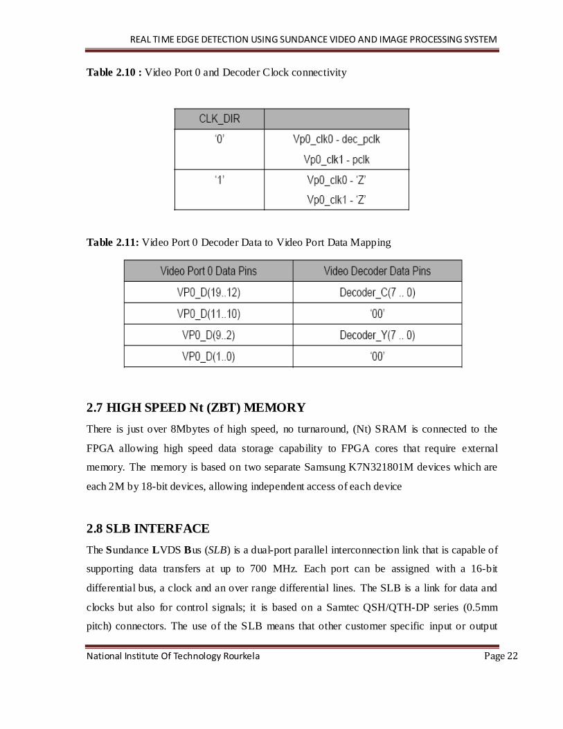
Table 2.10 : Video Port 0 and Decoder Clock connectivity

Table 2.11: Video Port 0 Decoder Data to Video Port Data Mapping

2.7 HIGH SPEED Nt (ZBT) MEMORY

There is just over 8Mbytes of high speed, no turnaround, (Nt) SRAM is connected to the

FPGA allowing high speed data storage capability to FPGA cores that require external

memory. The memory is based on two separate Samsung K7N321801M devices which are

each 2M by 18-bit devices, allowing independent access of each device

2.8 SLB INTERFACE

The Sundance LVDS Bus (SLB) is a dual-port parallel interconnection link that is capable of

supporting data transfers at up to 700 MHz. Each port can be assigned with a 16-bit

differential bus, a clock and an over range differential lines. The SLB is a link for data and

clocks but also for control signals; it is based on a Samtec QSH/QTH-DP series (0.5mm

pitch) connectors. The use of the SLB means that other customer specific input or output



methods can be supported without the need for re-design of the hardware. Some examples of

IO interfaces are listed below.

Input Output

• Camera Link • USB

• Firewire • IDE

• CMOS Sensor • Fiber Channel

• Fiber Channel • LCD/Plasma Display drivers

• DVI • DVI

2.9 VIDEO PORTS AND OTHERS MODULES

The SMT339 has 3 video ports connected from the DSP to the Virtex 4 FPGA. Video port 0

is, by default, routed to the video decoder and video port 1 is connected to the video

encoder. Video Port 1 is unused in the default FPGA configuration and is reserved for

upgraded firmware when the SMT339 is used with carrier boards such as the SMT114, or

SLB cards such as the SMT339. The port is reserved for either: an extra video input/output

or, the port is reserved for use as a SPI interface.

2.9.1 VIDEO ENCODER SETUP

The video encoder has a wide rage of operational features; such has output format, lookup

tables, and cursor insertion and colour space conversions. This section describes the basics

operation of the encoder. The figure below illustrates the flow from data in DSP memory to

final output by the encoder together with the necessary stages that require initialising.

Figure 2.3 : Flow from Video Memory to Encoder



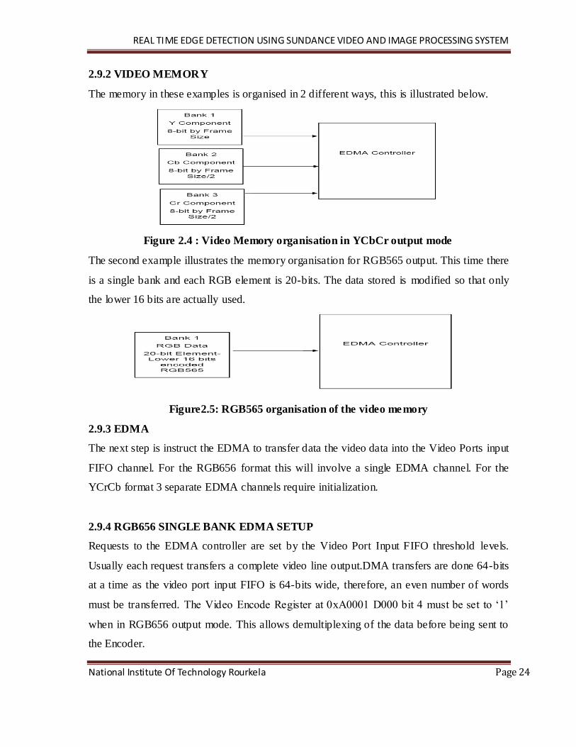
2.9.2 VIDEO MEMORY

The memory in these examples is organised in 2 different ways, this is illustrated below.

Figure 2.4 : Video Memory organisation in YCbCr output mode

The second example illustrates the memory organisation for RGB565 output. This time there

is a single bank and each RGB element is 20-bits. The data stored is modified so that only

the lower 16 bits are actually used.

Figure2.5: RGB565 organisation of the video memory

2.9.3 EDMA

The next step is instruct the EDMA to transfer data the video data into the Video Ports input

FIFO channel. For the RGB656 format this will involve a single EDMA channel. For the

YCrCb format 3 separate EDMA channels require initialization.

2.9.4 RGB656 SINGLE BANK EDMA SETUP

Requests to the EDMA controller are set by the Video Port Input FIFO threshold levels.

Usually each request transfers a complete video line output.DMA transfers are done 64-bits

at a time as the video port input FIFO is 64-bits wide, therefore, an even number of words

must be transferred. The Video Encode Register at 0xA0001 D000 bit 4 must be set to „1‟

when in RGB656 output mode. This allows demultiplexing of the data before being sent to

the Encoder.



2.9.5 BT656 WITH EMBEDDED SYNC EDMA SETUP

Three separate EDMA channels must me setup for this mode. One for the Y channel, one for

the Cr channel and one for the Cb channel.

The size of the EDMA is 180 (64bit transfers) for the Y channel which represent 720 pixels

(as data is transferred line by line). The Cb and Cr channels must be half of this representing

the chroma content of the YCrYCb data stream.

2.9.6 JTAG

There are two separate JTAG chains on the SMT339 module. One allows the DSP chain to

be accessed while the other allows the Virtex 4 to be configured.

1. DSP JTAG Chain

This is used by code composer studio to access the DSP. There is provision to extend the

number of processors in the chain by adding a DSP via a SLB mezzanine card. If this is

added then the SLB JTAG bypass jumper (JP3) should be removed.

2. Virtex 4 JTAG chain

This can be accessed via the JP5 connector using Xilinx tools.

JP1 - Flash Write Protect jumper – Fit to write enable

JP2 - Virtex Program Enable – Remove to Erase FPGA

JP3 - DSP JTAG chain –If removed the DSP JTAG chain is extended to a extra SLB

interface card DSP. Fit for normal operation.

2.9.7 CABELS AND CONNECTORS

Table 2.12: JP5 Virtex JTAG Header



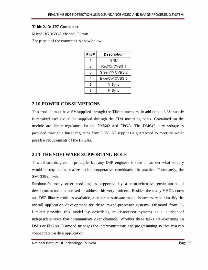
Table 2.13: JP7 Connector

Mixed RGB/VGA channel Output

The pinout of the connector is show below.

2.10 POWER CONSUMPTIONS

This module must have 5V supplied through the TIM connectors. In addition, a 3.3V supply

is required and should be supplied through the TIM mounting holes. Contained on the

module are linear regulators for the DM642 and FPGA. The DM642 core voltage is

provided through a linear regulator from 3.3V. All supplies a guaranteed to meet the worst

possible requirements of the FPGAs.

2.11 THE SOFTWARE SUPPORTING ROLE

This all sounds great in principle, but any DSP engineer is sure to wonder what sorcery

would be required to realize such a cooperative combination in practice. Fortunately, the

SMT339 (as with

Sundance‟s many other modules) is supported by a comprehensive environment of

development tools conceived to address this very problem. Besides the many VHDL cores

and DSP library modules available, a coherent software model is necessary to simplify the

overall application development for these mixed-processor systems. Diamond from 3L

Limited provides this model by describing multiprocessor systems as a number of

independent tasks that communicate over channels. Whether these tasks are executing on

DSPs or FPGAs, Diamond manages the interconnections and programming so that you can

concentrate on their application.



Diamond uses the FPGAs on Sundance DSP TIMs by automatically adding the engineer‟s

tasks to the standard Sundance firmware. These tasks are created in VHDL or tools such as

Xilinx System Generator, or they can be standard net list files, allowing you to bring

proprietary cores into the system and mix them with standard and user-developed cores.

Diamond automatically adds the logic to allow the tasks to communicate with other tasks; it

then builds an FPGA bit stream using the standard Xilinx tools.

This technique creates a hardware independence that allows you to make major changes to

the underlying hardware without having to change any code. It is now possible to expand the

hardware by adding DSPs or FPGAs as required, without so much as a recompilation.

Repositioning a task on a different DSP reduces to only a tiny change in a single text file.

Thus, when more processing power becomes necessary, you can add it at will, and none of

the existing development is made redundant. Even if a task needs to be moved from a DSP

to an FPGA for acceleration, the surrounding functions are not affected.

Chapter 3

EDGE DETECTION TECNIQUES

USING SUNDANCE MODULE



3.1 INTRODUCTION TO FUNDAMENTALS OF EDGE DETECTION

Edge detection refers to the process of identifying and locating sharp discontinuities in an

image. The discontinuities are abrupt changes in pixel intensity which characterize

boundaries of objects in a scene. Classical methods of edge detection involve convolving the

image with an operator (a 2-D filter), which is constructed to be sensitive to large gradients

in the image while returning values of zero in uniform regions. This is an extremely large

number of edge detection operators available, each designed to be sensitive to certain types

of edges. Variables involved in the selection of an edge detection operator include:

1) Edge orientation: The geometry of the operator determines a characteristic direction

in which it is most sensitive to edges. Operators can be optimized to look for

horizontal, vertical, or diagonal edges.

2) Noise environment: Edge detection is difficult in noisy images, since both the noise

and the edges contain high-frequency content. Attempts to reduce the noise result in

blurred and distorted edges. Operators used on noisy images are typically larger in

scope, so they can average enough data to discount localized noisy pixels. This

results in less accurate localization of the detected edges.

3) Edge structure: Not all edges involve a step change in intensity. Effects such as

refraction or poor focus can result in objects with boundaries defined by a gradual

change in intensity. The operator needs to be chosen to be responsive to such a

gradual change in those cases. Newer wavelet-based techniques actually characterize

the nature of the transition for each edge in order to distinguish, for example, edges

associated with hair from edges associated with a face.

There are many ways to perform edge detection. However, the majority of different methods

may be grouped into two categories:

Gradient: The gradient method detects the edges by looking for the maximum and

minimum in the first derivative of the image.

Laplacian: The Laplacian method searches for zero crossings [4] in the second

derivative of the image to find edges. An edge has the one-dimensional shape of a



ramp and calculating the derivative of the image can highlight its location. Suppose

we have the following signal, with an edge shown by the jump in intensity below:

Figure3.1: following signal apply to the edge detector

If we take the gradient of this signal (which, in one dimension, is just the first derivative

with respect to t) we get the following:

Figure3.2: the gradient first derivative signal

Clearly, the derivative shows a maximum located at the center of the edge in the original

signal. This method of locating an edge is characteristic of the “gradient filter” family of

edge detection filters and includes the Sobel method. A pixel location is declared an edge

location if the value of the gradient exceeds some threshold. As mentioned before, edges

will have higher pixel intensity values than those surrounding it. So once a threshold is set,

you can compare the gradient value to the threshold value and detect an edge whenever the

threshold is exceeded. Furthermore, when the first derivative is at a maximum, the second

derivative is zero. As a result, another alternative to finding the location of an edge is to

locate the zeros in the second derivative. This method is known as the Laplacian and the

second derivative [13] of the signal is shown below:



Figure3.3: the gradient second derivative signal

The purpose of detecting sharp changes in image brightness is to capture important events

and changes in properties of the world. It can be shown that under rather general

assumptions for an image formation model, discontinuities in image brightness are likely to

correspond to:

I. discontinuities in depth,

II. discontinuities in surface orientation,

III. changes in material properties and

IV. Variations in scene illumination.

In the ideal case, the result of applying an edge detector to an image may lead to a set of

connected curves that indicate the boundaries of objects, the boundaries of surface markings

as well curves that correspond to discontinuities in surface orientation. Thus, applying an

edge detector to an image may significantly reduce the amount of data to be processed and

may therefore filter out information that may be regarded as less relevant, while preserving

the important structural properties of an image. If the edge detection step is successful, the

subsequent task of interpreting the information contents in the original image may therefore

be substantially simplified. Unfortunately, however, it is not always possible to obtain such

ideal edges from real life images of moderate complexity. Edges extracted from non-trivial

images are often hampered by fragmentation, meaning that the edge curves are not

connected, missing edge segments as well as false edges not corresponding to interesting

phenomena in the image -- thus complicating the subsequent task of interpreting the image

data.



3.2 A SIMPLE EDGE MODEL

Although certain literature has considered the detection of ideal step edges, the edges

obtained from natural images are usually not at all ideal step edges. Instead they are

normally affected by one or several of the following effects:

focal blur caused by a finite depth-of-field and finite point spread function.

Penumbral blur caused by shadows created by light sources of non-zero radius.

Shading at a smooth object edge.

local specularities or interreflections in the vicinity of object edges.

Although the following model does not capture the full variability of real- life edges, the

error function erf has been used by a number of researchers as the simplest extension of the

ideal step edge model for modeling the effects of edge blur in practical applications. Thus, a

one-dimensional image f which has exactly one edge placed at x = 0 may be modeled as:

At the left side of the edge, the intensity is , and right of the edge it is

. The scale parameter σ is called the blur scale of the edge.

(a) (b)

Figure3.4: Example of different types of edges



3.3 EDGE DETECTION

We‟ve discussed smoothing and diffusion as a way of getting rid of the effects of noise in an

image. Now we‟re going to discuss the problem of finding the boundaries between piece-

wise constant regions in the image, when these regions have been corrupted by noise. As

usual, we will begin by considering a 1D problem. But in the case of edge detection, we‟ll

also have to discuss the 2D problem, because there are some issues that arise in 2D that

don‟t show up in 1D.

1. 1D Edge Detection

1D edge detection consists of three, key steps.

a. Reduce the effects of noise.

b. Measure the magnitude of change in the region.

c. Find peaks of change

i. Non-maximum suppression

ii. Thresholding

The logic of this is that we need to avoid the effects of noise, and then we need to measure

the amount of change in intensity in the image, so that we can find places where intensity is

changing rapidly. We want to find peaks, because in the neighborhood of an edge, after

smoothing, there may be many pixels where the image is changing rapidly, but we only want

to identify one of them as the edge.

We have already discussed (1), reducing the effects of noise with smoothing. We also need

to consider how to do convolution discretely. One way to do this is to sample the filter (eg.,

sample the values of a Gaussian at some discrete points). One must be careful about two

things:

1. Normalize the sampled Gaussian, so that it sums to 1.

2. Be sure to use a wide enough filter to capture the Gaussian shape. This is done heuristically,

but is important.

We mention that Canny has considered the question of finding the optimal way to smooth a

noisy step edge in order to find edges, and has found that the optimal smoothing function

[3][6][7] is approximately a Gaussian. Canny defined optimality by defining some



reasonable criteria, such as accurate localization and lack of false positives. We also mention

that it is particularly important to reduce the effects of noise before taking a derivative. One

way to justify this is to note that white noise has a uniform power spectrum, while scene

structure is usually more low frequency than high frequency. A derivative is a high-pass

filter. So the derivative preserves the noise much more than the structure. The way to avoid

this is to low-pass filter the image first, which removes noise much more than it removes

structure. In 1D, it is easy to measure the amount of change. The way that we measure

change is by taking a derivative.

Finding peaks is also simple.

1) We look for points where the magnitude of the derivative is bigger than at the two

neighboring points. (We could also look for places where the second derivative is 0,

although this is slightly trickier in the discrete case). This is called non-maximum

suppression [10] and is equivalent to finding the place where the first derivative is a

maximum.

2) We also look for peaks where the magnitude of the first derivative is above some

threshold. This eliminates spurious edges.

2. 2D Edge Detection

We perform Edge Detection by performing essentially the same steps. However, some of

these steps will look a little different in 2D.

1) Reduce the effects of noise. This is exactly the same. I am smoothing with a Gaussian. The

only difference is that I am using a 2D Gaussian. One useful thing to note, though, is that we

can decompose a 2D Gaussian into two 1D Gaussians, which improves efficiency.

2) Measure the magnitude of change in the region. In 1D we measure change with a

derivative. In 2D, we measure change with a gradient. This is a 2D vector. We produce it by

combining the partial derivative in the x and y directions. The direction of the gradient

provides the direction of maximum change. The magnitude of the gradient tells us how fast

the image is changing if we move in that direction. One way to think about this is that when



we take the gradient, we are just looking at first order properties of the intensities. That

means that we can approximate the intensities as locally linear. So think of them as lying in

a plane. The gradient tells us the direction the plane is tilted, and how much it is tilted.

3) Find peaks of change

a) Non-maximum suppression. This is a lot more complicated than in 1D.We don‟t just want to

look at local maxima. First of all, that would be silly, because the boundaries of objects in

2D are 1D curve, whereas local maxima would be isolated points. Consider a simple ca se of

a white square on a black background. The gradient magnitude will be constant along the

edge, and will be decreasing in the direction orthogonal to the edge. So we look for points

that are maxima in the direction of the gradient. We must interpolate when the gradient

doesn‟t point directly to a pixel.

b) Thresholding - An innovation of Canny was to use two thresholds (hysteresis).

A high threshold. All maxima with gradient magnitudes above that are edges.

A low threshold. All maxima above this are edges if they are also connected to an edge.

Note that this is a recursive definition [2].

3.4 THE FOUR STEPS OF EDGE DETECTION

(1) Smoothing: suppress as much noise as possible, without destroying the true edges.

(2) Enhancement: apply a filter to enhance the quality of the edges in the image (sharpening).

(3) Detection: determine which edge pixels should be discarded as noise and which should be

retained (usually, thresholding provides the criterion used for detection).

(4) Localization: determine the exact location of an edge (sub-pixel resolution might be

required for some applications, that is, estimate the location of an edge to better than the

spacing between pixels). Edge thinning and linking are usually required in this step.



3.5 EDGE DETECTION USING DERIVATIVES

Calculus describes changes of continuous functions using derivatives. An image is a

2D function, so operators describing edges are expressed using partial derivatives. Points

which lie on an edge can be detected by:

(1) Detecting local maxima or minima of the first derivative.

(2) Detecting the zero-crossing of the second derivative

Figure3.5: Edge Detection Using Derivatives

Differencing 1D signals

To compute the derivative of a signal, we approximate the derivative by finite differences:

Computing the 1st derivative:

)1)(()()()(

lim)('0

hxfhxfh

xfhxfxf

h

mask: [ -1 1]

Examples using the edge models and the mask [ -1 0 1] (centered about x):

Mask M : [ -1 1]



S1 12 12 12 12 12 24 24 24 24 24

S1 M 0 0 0 0 12 12 0 0 0 0

(a) S1 is upward step edge

S2 24 24 24 24 24 12 12 12 12 12

S2 M 0 0 0 0 -12 -12 0 0 0 0

(b) S2 is downward step edge

S3 12 12 12 12 15 18 21 24 24 24

S3 M 0 0 0 3 6 6 6 3 0 0

(c) S3 is an upward ramp

S4 12 12 12 12 24 12 12 12 12 12

S4 M 0 0 0 12 0 -12 0 0 0 0

(d) S4 is an upward ramp

Computing the 2nd derivative:

)(')(')(')('

lim)(''0

xfhxfh

xfhxfxf

h

)1)(()1(2)2( hxfxfxf

This approximation is centered about x + 1; by replacing x + 1 by x we obtain:

)1()(2)1()('' xfxfxfxf

mask: [ 1 -2 1]

- Examples using the edge models:



Mask M : [ -1 1]

S1 12 12 12 12 12 24 24 24 24 24

S1 M 0 0 0 0 -12 12 0 0 0 0

(a) S1 is upward step edge

S2 24 24 24 24 24 12 12 12 12 12

S2 M 0 0 0 0 12 -12 0 0 0 0

(b) S2 is downward step edge

S3 12 12 12 12 15 18 21 24 24 24

S3 M 0 0 0 -3 0 0 0 3 0 0

(c) S3 is an upward ramp

S4 12 12 12 12 24 12 12 12 12 12

S4 M 0 0 0 -12 24 -12 0 0 0 0

(d) S4 is an upward ramp

3.6 EDGE DETECTION USING THE GRADIENT

3.6.1 Definition of the gradient

- The gradient is a vector which has certain magnitude and direction:

y

f

x

f

f

22

22

)( yx MMy

f

x

ffmagn



)(tan)( 1

x

y

M

Mfdir

- To save computations, the magnitude of gradient is usually approximated by:

yx MMfmagn )(

3.6.2 Properties of the gradient

1. The magnitude of gradient provides information about the strength of the edge.

2. The direction of gradient is always perpendicular to the direction of the edge (the edge

direction is rotated with respect to the gradient direction by -90 degrees).

Figure3.6: the edge direction is rotated with respect to the gradient direction by -90 degrees

3.6.3 Estimating the gradient with finite differences

h

yxfyhxf

x

f

h

),(),(lim

0

h

yxfhyxf

y

f

h

),(),(lim

0

The gradient can be approximated by finite differences:

)1(),,()1,(),(),(

)1(),,(),1(),(),(

y

y

y

x

x

x

hyxfyxfh

yxfhyxf

y

f

hyxfyxfh

yxfyhxf

x

f

Using pixel-coordinate notation (remember: j corresponds to the x direction and i to the

negative y direction):



),()1,( jifjifx

f

),1(),(),(),1( jifjify

forjifjif

y

f

3.7 DIFFERENT TYPE EDGE DETECTOR

Edge detection is a terminology in image processing and computer vision, particularly in

the areas of feature detection [8] and feature extraction [23], to refer to algorithms which

aim at identifying points in a digital image at which the image brightness changes sharply or

more formally has discontinuities. they are many type but I am using only four types of edge

detector that is

1. Sobel Edge Detector - 3×3 gradient edge detector

2. Prewitt Edge Detector - 3×3 gradient edge detector

3. Canny Edge Detector - non-maximal suppression of local gradient magnitude

4. Zero Crossing Detector - edge detector using the Laplacian of Gaussian operator

3.7.1 Sobel Edge Detector

The Sobel operator [15] performs a 2-D spatial gradient measurement on an image and so

emphasizes regions of high spatial frequency that correspond to edges. Typically it is used to find

the approximate absolute gradient magnitude at each point in an input grayscale image.

3.7.1.1 How It Works

In theory at least, the operator consists of a pair of 3×3 convolution kernels as shown in

Figure shown one kernel is simply the other rotated by 90°.



Figure3.7: Sobel convolution kernels

These kernels are designed to respond maximally to edges running vertically and horizontally

relative to the pixel grid, one kernel for each of the two perpendicular orientations. The kernels can

be applied separately to the input image, to produce separate measurements of the gradient

component in each orientation (call these Gx and Gy). These can then be combined together to find

the absolute magnitude of the gradient at each point and the orientation of that gradient. The

gradient magnitude is given by:

22GyGxG

Typically, an approximate magnitude is computed using:

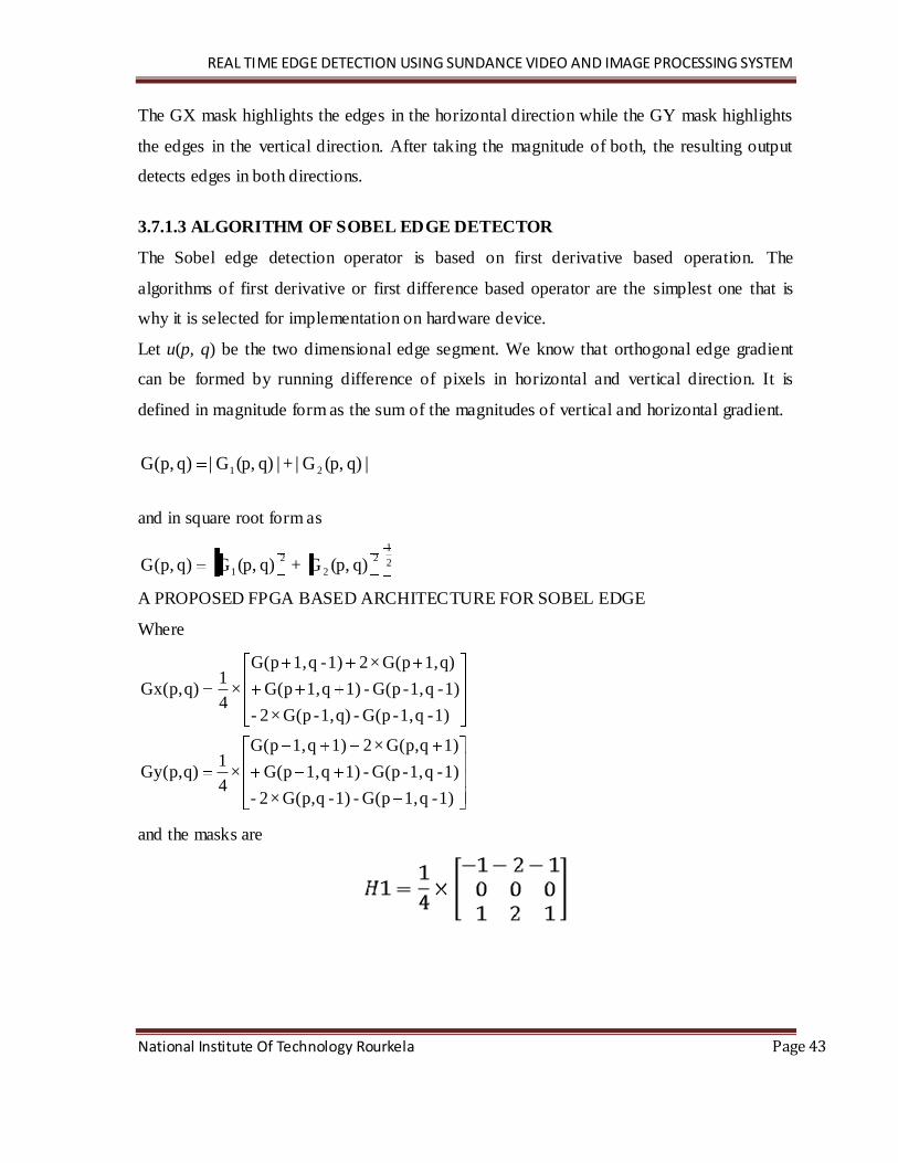
| G |=| Gx | +| Gy|

which is much faster to compute.

The angle of orientation of the edge (relative to the pixel grid) giving r ise to the spatial

gradient is given by:

θ =tan-1

(Gy/Gx)

In this case, orientation 0 is taken to mean that the direction of maximum contrast from

black to white runs from left to right on the image, and other angles are measured anti-

clockwise from this. Often, this absolute magnitude is the only output the user in the two

components of the gradient are conveniently computed and added in a single pass over the

input image using the pseudo-convolution operator shown in Figure shown below.



Figure3.8: Pseudo-convolution kernels used to quickly compute approximate gradient magnitude

Using this kernel the approximate magnitude is given by:

| G | =| (P1+2×P2+P3)-(P7+2×P8+P9) |+ | (P3+2×P6+P9)-(P1+2×P4+P7) |

3.7.1.2 Sobel Explanation

The mask is slid over an area of the input image, changes that pixel's value and then shifts

one pixel to the right and continues to the right until it reaches the end of a row. It then starts

at the beginning of the next row. The example below shows the mask being slid over the top

left portion of the input image represented by the green outline. The formula shows how a

particular pixel in the output image would be calculated. The center of the mask is placed

over the pixel you are manipulating in the image. And the I & J values are used to move the

file pointer so you can multiply, for example, pixel (a22) by the corresponding mask value

(m22). It is important to notice that pixels in the first and last rows, as well as the first and

last columns cannot be manipulated by a 3x3 mask. This is because when placing the center

of the mask over a pixel in the first row (for example), the mask will be outside the image

boundaries.

Figure3.9: Sobel Explanation how to get output b22



The GX mask highlights the edges in the horizontal direction while the GY mask highlights

the edges in the vertical direction. After taking the magnitude of both, the resulting output

detects edges in both directions.

3.7.1.3 ALGORITHM OF SOBEL EDGE DETECTOR

The Sobel edge detection operator is based on first derivative based operation. The

algorithms of first derivative or first difference based operator are the simplest one that is

why it is selected for implementation on hardware device.

Let u(p, q) be the two dimensional edge segment. We know that orthogonal edge gradient

can be formed by running difference of pixels in horizontal and vertical direction. It is

defined in magnitude form as the sum of the magnitudes of vertical and horizontal gradient.

|q) (p,G| + |q) (p,G| )q p,(G 21

and in square root form as

q) (p,G + q) (p,G )q p,(G 2

12

2

2

1

A PROPOSED FPGA BASED ARCHITECTURE FOR SOBEL EDGE

Where

1)-q1,G(p-1)-qG(p, × 2-

1)-q1,-G(p-1)q1,G(p

1)qG(p, × 21)q1,G(p

× 4

1q) Gy(p,

1)-q1,-G(p-q)1,-G(p × 2-

1)-q1,-G(p-1)q1,G(p

q)1,G(p × 21)-q1,G(p

× 4

1q) Gx(p,

and the masks are



The weights used in the horizontal and vertical neighborhood are used for noise smoothing

by giving more importance to neighborhood pixels. The reason for choosing 3 × 3

neighborhood is to make the operator less sensitive to noise. This operator performs

differencing in one dimension and weighted spatial averaging in another for getting

smoothed edge. Sobel masks are the combination of smoothing and difference operator:

*

And

*

3.7.1.4 PROPOSED ARCHITECTURE

The proposed architecture is shown in Figure3.10. The input to this scheme is eight eight-bit

pixel values coming through eight bytes bus and eight-bit threshold value for comparison

with gradient. The output to this scheme is edge detected pixel value in the form of either

eight-bit zeros or eight-bit 255, depending on the value of threshold supplied as the eight-bit

input. The various blocks constituting this architecture are:

Figure3.10: Proposed architecture for sobel edge detection operator.



Decoder Block

The function of this block is to take eight pixel values and decode it into twelve pixel values

to route into four-processing blocks, three pixels per processing block.

First Processing Block

This block applies the weights −1,−2 and −1 to the three pixel values coming to it. After

completing addition of weighted-pixel values, down scaling of resultant by a factor of four is

performed.

Second Processing Block

The function of this block is to apply weights of 1, 2, and 1 to the three pixel values coming

to it. After completing addition of weighted-pixel values, division of resultant by a factor of

four is performed.

Third Processing Block

The function of this block is similar to first processing block.

Fourth Processing Block

The function of this block is similar to second processing block.

Adder Divider Blocks

The function of these blocks is to add the two pixel values coming to them from the four

processing blocks. After addition the resultant is divided by two.

Final Adder Divider Block

The function of this block is to add the two eight-bit pixel values coming to it from the two

adders block. After addition division by a factor of two is performed.

Comparator Block

The comparison of the resultant gradient value from a given threshold value is performed by

this block. The final result is the edge-detected binary image having only two pixel values,

i.e., 0 and 255.



3.7.2 Prewitt Edge Detector

A related operator is the Prewitt gradient edge detector [15][29] (not to be confused with the

Prewitt compass edge detector). This works in a very similar way to the Sobel operator but

uses slightly different kernels, as shown in Figure shown below. This kernel produces

similar results to the Sobel, but is not as isotropic in its response.

Figure3.11: Masks for the Prewitt gradient edge detector.

The gradient magnitude is given by:

22GyGxG

Typically, an approximate magnitude is computed using:

| G |=| Gx | +| Gy|

The angle of orientation of the edge (relative to the pixel grid) giving rise to the spatial

gradient is given by:

θ =tan-1

(Gy/Gx)

NOTE- Implemation of Prewitt operator is same applied to the sobel operator.



3.7.2.1 Result of Sobel and Prewitt Operator

a) Original image

b) Prewitt Operator c) Sobel Operator

Figure3.12: Result of Sobel and Prewitt Operator



3.7.3 Canny Edge Detector

Edges characterize boundaries and are therefore a problem of fundamental importance in

image processing. Edges in images are areas with strong intensity contrasts – a jump in

intensity from one pixel to the next. Edge detecting an image significantly reduces the

amount of data and filters out useless information, while preserving the important structural

properties in an image.

The Canny edge detection algorithm is known to many as the optimal edge detector. Canny's

intentions were to enhance the many edge detectors already out at the time he started his

work. He was very successful in achieving his goal and his ideas and methods can be found

in his paper, "A Computational Approach to Edge Detection"[1]. He followed a list of

criteria to improve current methods of edge detection. The first and most obvious is low

error rate. It is important that edges occurring in images should not be missed and that there

be NO responses to non-edges. The second criterion is that the edge points be well localized.

In other words, the distance between the edge pixels as found by the detector and the actual

edge is to be at a minimum. A third criterion is to have only one response to a single edge.

This was implemented because the first 2 were not substantial enough to completely

eliminate the possibility of multiple responses to an edge.

Based on these criteria, the canny edge detector first smoothes the image to eliminate and

noise. It then finds the image gradient to highlight regions with high spatial derivatives. The

algorithm then tracks along these regions and suppresses any pixel that is not at the

maximum (nonmaximum suppression). The gradient array is now further reduced by

hysteresis. Hysteresis is used to track along the remaining pixe ls that have not been

suppressed. Hysteresis uses two thresholds and if the magnitude is below the first threshold,

it is set to zero (made a nonedge). If the magnitude is above the high threshold, it is made an

edge. And if the magnitude is between the 2 thresholds, then it is set to zero unless there is a

path from this pixel to a pixel with a gradient above T2.



Step-1

In order to implement the canny edge detector algorithm, a series of steps must be followed.

The first step is to filter out any noise in the original image before trying to locate and detect

any edges. And because the Gaussian filter can be computed using a simple mask, it is used

exclusively in the Canny algorithm. Once a suitable mask has been calculated, the Gaussian

smoothing can be performed using standard convolution methods. A convolution mask is

usually much smaller than the actual image. As a result, the mask is slid over the image,

manipulating a square of pixels at a time. The larger the width of the Gaussian mask, the

lower is the detector's sensitivity to noise. The localization error in the detected edges also

increases slightly as the Gaussian width is increased. The Gaussian mask used in my

implementation is shown below.

Figure3.13: Discrete Approximation to Gaussian function with σ=1.4

Step-2

After smoothing the image and eliminating the noise, the next step is to find the edge

strength by taking the gradient of the image. The Sobel operator performs a 2-D spatial

gradient measurement on an image. Then, the approximate absolute gradient magnitude

(edge strength) at each point can be found. The Sobel operator uses a pair of 3x3

convolution masks, one estimating the gradient in the x-direction (columns) and the other

estimating the gradient in the y-direction (rows). They are shown below:

Figure3.14: The Sobel operator uses a pair of 3x3 convolution masks



The magnitude, or EDGE STRENGTH, of the gradient is then approximated using the

formula:

|G| = |Gx| + |Gy|

Step-3

Finding the edge direction is trivial once the gradient in the x and y directions are known.

However, you will generate an error whenever sumX is equal to zero. So in the code there

has to be a restriction set whenever this takes place. Whenever the gradient in the x direction

is equal to zero, the edge direction has to be equal to 90 degrees or 0 degrees, depending on

what the value of the gradient in the y-direction is equal to. If GY has a value of zero, the

edge direction will equal 0 degrees. Otherwise the edge direction will equal 90 degrees. The

formula for finding the edge direction is just:

θ = tan-1

(Gy / Gx)

Step-4

Once the edge direction is known, the next step is to relate the edge direction to a direction

that can be traced in an image. So if the pixels of a 5x5 image are aligned as follows:

x x x x x

x x x x x

x x a x x

x x x x x

x x x x x

Then, it can be seen by looking at pixel "a", there are only four possible directions when

describing the surrounding pixels - 0 degrees (in the horizontal direction), 45 degrees

(along the positive diagonal), 90 degrees (in the vertical direction), or 135 degrees (along

the negative diagonal). So now the edge orientation has to be resolved into one of these four

directions depending on which direction it is closest to (e.g. if the orientation angle is found



to be 3 degrees, make it zero degrees). Think of this as taking a semicircle and dividing it

into 5 regions.

Figure3.15: The Orientation Angle is Found to be 3 Degrees

Therefore, any edge direction falling within the yellow range (0 to 22.5 & 157.5 to 180

degrees) is set to 0 degrees. Any edge direction falling in the green range (22.5 to 67.5

degrees) is set to 45 degrees. Any edge direction falling in the blue range (67.5 to 112.5

degrees) is set to 90 degrees. And finally, any edge direction falling within the red range

(112.5 to 157.5 degrees) is set to 135 degrees.

Step-5

After the edge directions are known, nonmaximum suppression now has to be applied.

Nonmaximum suppression is used to trace along the edge in the edge direction and suppress

any pixel value (sets it equal to 0) that is not considered to be an edge. This will give a thin

line in the output image.

Step-6

Finally, hysteresis is used as a means of eliminating streaking. Streaking is the breaking up

of an edge contour caused by the operator output fluctuating above and below the threshold.

If a single threshold, T1 is applied to an image, and an edge has an average strength equal to

T1, then due to noise, there will be instances where the edge dips below the threshold.

Equally it will also extend above the threshold making an edge look like a dashed line. To

avoid this, hysteresis uses 2 thresholds, a high and a low. Any pixel in the image that has a

value greater than T1 is presumed to be an edge pixel, and is marked as such immediately.

Then, any pixels that are connected to this edge pixel and that have a value greater than T2

are also selected as edge pixels. If you think of following an edge, you need a gradient of T2

to start but you don't stop till you hit a gradient below T1.



3.7.3.1 Canny Edge Detection algorithms

This is a multi-step edge detection procedure by Canny [33]. The purpose of the following

two methods is to detect edges with noise suppressed at the same time.

1. Smooth the image with a Gaussian filter to reduce noise and unwanted details and

textures.

Where

Compute gradient of g(m ,n) using any of the gradient operators ( Sobel, Prewitt,

etc) to get:

(m,n)g(m,n)gM(m,n) nm22

and

2. Threshold M:

where T is so chosen that all edge elements are kept while most of the noise is

suppressed.



3. Suppress non-maxima pixels in the edges in MT obtained above to thin the edge

ridges (as the edges might have been broadened in step 1). To do so, check to see

whether each non-zero MT (m, n) is greater than its two neighbors along the gradient

direction θ(m, n). If so, keep M T (m, n) unchanged, otherwise, set it to 0.

4. Threshold the previous result by two different thresholds T1 and T2 (where T1< T2) to

obtain two binary images T1 and T2. Note that compared to T1, T2 has less noise and

fewer false edges but larger gaps between edge segments.

5. Link edges segments in T2 to form continuous edges. To do so, trace each segment in

T2 to its end and then search its neighbors in T1 to find any edge segment in T1 to

bridge the gap until reaching another edge segment in T2.

3.7.3.2 Implementation on an FPGA

The schematic of the canny edge detection is shown in Figure

Figure3.16: Block diagram implementation of Canny algorithm

The FPGA implementation of the Canny edge-detector algorithm is partitioned into four

different stages as shown in Figure 3.15.

Figure 3.16 describes the implementation of a generic non-symmetric 2-D image filter. The

incoming pixels are shifted through the line buffers that create a delay line. The buffer depth

depends on the number of pixels in each line of the frame. These delay lines feed the filter

array simultaneously with pixels from all the relevant video lines. At each filter node, the

pixel is multiplied with the appropriate filter coefficients. All the multiplier results are added



together at the adder tree to produce the filter middle point output result. Typically, scaling

is applied at the final output.

Figure3.17: Hardware Implementation of non-symmetric 2D filter

In general, the efficiency of a hardware implementation is measured by the number of

multiplications. Using this metric as the measure, the complexity of the nonsymmetric filter

is proportional to the dimension of the filter m2, where m * m is the size of the convolutional

kernel.

Significant size optimization can be achieved in the case of symmetric 2-D video filters. The

optimization is even more significant in cases where the filter kernel is symmetric and

separable, as is the case with the Gaussian filter used in the Canny algorithm. The 2-D filter

is separated into two 1-D filters implemented first in the horizontal direction, followed by

the vertical direction as shown in Figure 3.17. This technique can be applied to both the

smoothing stage with the Gaussian filter, and the identification of the gradient with the

derivative of the Gaussian. Table 1 shows the implementation complexity of the different

class of filters as a function of number of multiplication operations.

Table 1: 2-D Filter implementation complexity based on number of multiplication

operations



Figure 3.18: Hardware implementation of symmetric separable 2D filter

Since the convolution for both the Gaussian and its derivative can be implemented as

separate 1-D convolutions, the operations are implemented in parallel on the FPGA as

shown in Figure 3.15. The noise reduction function is performed using a 7*7 Gaussian

kernel. This kernel slides over the image, line by line, attenuating the high-frequency noise

components of the image. The finding of zero crossings is performed using a 5*5 kernel

obtained by calculating the derivative of Gaussian. The non-maximal suppression stage

identifies pixels that are local maxima in the direction of the gradient using the magnitude

and orientation of the pixels. The major orientation of the gradient, either horizontal or

vertical, is obtained by comparing the individual components, dx and dy, which are the

result of convolving the smoothed image with the derivative of the Gaussian. Since most

edges are at an angle, it is possible to obtain further granularity in the orientation of the

gradient by comparing the sign bit of the gradient . This allows the neighboring pixels and

the orientation of the gradient to be determined within specific quadrants as shown in Figure

3.18.

Figure 3.19: Determine orientation of gradient in the nonmaximal suppression stage



the gradient is compared to the interpolated value of the magnitude of the neighboring

pixels.

The magnitude of the neighboring pixels is calculated using parallel multiplier units. Pixels

with gradient intensities less than their neighboring pixels in the gradient direction are

automatically suppressed or classified as a non-edge in order to keep the edges thin.

The final stage involves thresholding the result from the non-maximal suppression stage to

create a binary image using two threshold values (hysteresis): TH and TL.A straightforward

approach would include running a first pass over the video frame to compare all the pixels

with the two threshold values. Pixels with gradient values above TH are marked „2‟,

classified as an edge. Next, pixels with gradient values less than TH but above TL are marked

„1‟, classified as a potential edge. The rest of the pixels are left as zeros, or non-edge. Figure

3.19 shows an example of this frame mapping approach. For each pixel marked as „2‟, its

neighboring pixels within a 3x3 neighborhood that are marked „1‟ are remarked „2‟. If

implemented in software, this section of the algorithm alone can contribute to more than 20

operations per pixel. Additional passes are required to find potential edges that were left

behind in the initial passes. Edges are left behind in cases where there is a line of „1‟s that

leads to „2‟ in the direction of the pass. Figure 3.20 shows an example with the assumption

that the lines are processed from left to right starting at the top. In this scenario, all the „1‟s

in the second row would be remarked as „2‟ only in subsequent passes. The number of

passes required depends on the characteristics of each video frame.

Figure 3.20: Edge strength classification map



3.7.3.3 Result of Canny Operator

a) Original image

b) Canny Operator

Figure 3.21: Result of Canny Operator



3.7.4 Laplacian of Gaussian

The Laplacian is a 2-D isotropic measure of the 2nd spatial derivative of an image. The

Laplacian of an image highlights regions of rapid intensity change and is therefore often

used for edge detection. The Laplacian is often applied to an image that has first been

smoothed with something approximating a Gaussian Smoothing filter in order to reduce its

sensitivity to noise. The operator normally takes a single gray level image as input and

produces another gray level image as output.

The Laplacian L(x,y) of an image with pixel intensity values I(x,y) is given by:

2

2

2

2

y

I

x

Iy)L(x,

Since the input image is represented as a set of discrete pixels, we have to find a discrete

convolution kernel that can approximate the second derivatives in the definition of the

Laplacian. Three commonly used small kernels are shown in Figure.

Figure 3.22: Three commonly used discrete approximations to the Laplacian filter.

Because these kernels are approximating a second derivative measurement on the image,

they are very sensitive to noise. To counter this, the image is often Gaussian Smoothed

before applying the Laplacian filter [27]. This pre-processing step reduces the high

frequency noise components prior to the differentiation step.

In fact, since the convolution operation is associative, we can convolve the Gaussian

smoothing filter with the Laplacian filter first of all, and then convolve this hybrid filter with

the image to achieve the required result. Doing things this way has two advantages:

http://homepages.inf.ed.ac.uk/rbf/HIPR2/gsmooth.htm



1. Since both the Gaussian and the Laplacian kernels are usually much smaller than the

image, this method usually requires far fewer arithmetic operations.

2. The LoG (`Laplacian of Gaussian') kernel can be precalculated in advance so only

one convolution needs to be performed at run-time on the image.

The 2-D LoG function centered on zero and with Gaussian standard deviation σ has the

form:

22σ

2y

2x

e2

2σ

2y

2x

14

πσ

1y)LoG(x,

and is shown in Figure

Figure 3.23: The 2-D Laplacian of Gaussian (LoG) function. The x and y axes are marked

in standard deviations (σ)

Figure 3.24: Discrete approximation to LoG function with Gaussian σ = 1.4



Note that as the Gaussian is made increasingly narrow, the LoG kernel becomes the same as

the simple Laplacian kernels shown in Figure3.22. This is because smoothing with a very

narrow Gaussian (σ< 0.5 pixels) on a discrete grid has no effect. Hence on a discrete grid,

the simple Laplacian can be seen as a limiting case of the LoG for narrow Gaussians. The

LoG operator calculates the second spatial derivative of an image. This means that in areas

where the image has a constant intensity (i.e. where the intensity gradient is zero), the LoG

response will be zero. In the vicinity of a change in intensity, however, the LoG response

will be positive on the darker side, and negative on the lighter side. This means that at a

reasonably sharp edge between two regions of uniform but different intensities, the LoG

response will be:

1. zero at a long distance from the edge,

2. positive just to one side of the edge,

3. negative just to the other side of the edge,

4. Zero at some point in between, on the edge itself.

Figure 3.25 illustrates the response of the LoG to a step edge.

Figure 3.25: Response of 1-D LoG filter to a step edge. The left hand graph shows a 1-D

image, 200 pixels long, containing a step edge. The right hand graph shows the response of a

1-D LoG.



3.7.4.1 Result of Laplacian operator

a) Original b) Laplacian Operator

Figure 3.26: Result of Laplacian operator

Chapter 4

RESULT AND DISCUSSION



4.1 RESULT OF THE DIFFERENT OPERATOR

a) Original image

b) Prewitt Operator c) Sobel Operator



d) Canny Operator

e) Laplacian Operator

Figure 4.1: Result of the all the operator



4.2 COMPARISSION AND DISCUSSION

Figure shows through the edges for the different operators. The focus in the detection of the

edges that produces representing the original image. This provides a foundation for selecting

an appropriate edge detector for further application. Investigation is aimed at aiding the

choice of an appropriate operator that is capable of detecting boundaries based on intensity

discontinuities. The Sobel and Prewitt both are differencing and smoothing. It detects part of

the edges in the original image. The problem with these detectors is that it relies on finding

edges which fails to detect fine edges.

The Laplacian respond to transitions in intensity. As a second order derivative, the Laplacian

is sensitive to noise. Moreover the Laplacian produces double edges and is sometimes

unable to detect edge direction.

The canny edge detector is capable of reducing noise. The canny operator works in a

multistage process. These can be summarized in a smoothing with a Gaussian filter.

Followed by gradient computation and use of a double threshold. The canny produces the

best edge map.

The result is show that the behavior of zero crossing operator and gradient operator on the

capability of edge detection. The objective is to investigate the effect of the various methods

applied in finding edges of the image. It can show clearly that the Sobel and Prewitt low

quality edges as compared to other two detectors. A representation of the image can be

obtained through the canny and Laplacian of Gaussian method. Among the various methods

investigate the canny method is able to detect both strong and week edges and seems to be

more suitable than the Laplacian of Gaussian.

As edge detection is a fundamental step, it is necessary to point out the true edges to get the

best results from the matching process. That is why it is important to choose edge detectors

that fit best to the application. In this respect, we present some advantages and

disadvantages of algorithms within the context of our classification as follows:



1) Sobel and Prewitt :

Advantages:

1) Simple to understand and implement

2) Detection of edges and their orientations

Disadvantages:

1) Sensitive to noise,

2) Inaccurate

2) Laplacian operator:

Advantages:

1) Finding the correct places of edges,

2) Testing wider area around the pixel

Disadvantages:

1) Malfunctioning at corners, curves and where the gray level intensity function varies,

2) Not finding the orientation of edge because of using the Laplacian filter

3) Canny operator:

Advantages:

1) Using probability for finding error rate,

2) Localization and response,

3) Improving signal to noise ratio,

4) Better detection specially in noise conditions

Disadvantages:

1) Complex Computations,

2) False zero crossing,

3) Time consuming

Chapter 5

CONCLUSIONS AND

SCOPE OF FUTURE WORK



5.1 CONCLUSION

Edge detection is an important pre-processing step in image analysis. Edge detection is an

important work for object recognition and is also an essential pre-processing step in image

segmentation. These edge detection operators can have better edge effect under the

circumstances of obvious edge and low noise. There are various edge detection methods in the

domain of image edge detection, each having certain disadvantages. Hence we will acquire

satisfactory result if choosing suitable edge detection operator according to specific situation in

practice.

The subtle art of combining the respective strengths of FPGAs and DSPs can be

simplified by starting with a scalable system whose delicate integration is already complete.

Supported by a comprehensive software environment, such complex hardware can become both

adaptable and accessible, allowing its collective power to be finely tuned to the desired

application. After the solution is developed, with such a modular approach, you can then create a

production system efficiently from off the shelf modules.

5.2 Future Scope

In this thesis work, many existing detector are simulated and many edge detector through have

proposed for suppression image noise. The performance of proposed edge detector can be

improved by applying different filtering technique throughout the image in recursive way.

Because this is a new way of image and video processing through Sundance Module SMT339

and research in field of image processing are not yet fully explored. There are sufficient scope

for develop image and video processing by using Sundance Module SMT339 in the direction of

mentioned below.

1. In computer vision and image processing the concept of feature detection refers

to methods that aim at computing abstractions of image information and making

local decisions at every image point whether there is an image feature of a given

type at that point or not. The resulting features will be subsets of the image



domain, often in the form of isolated points, continuous curves or connected

regions. Since features are used as the starting point and main primitives for

subsequent algorithms, the overall algorithm will often only be as good as its

feature detector. Consequently, the desirable property for a feature detector is

repeatability: whether or not the same feature will be detected in two or more

different images of the same scene.

2. Video compression refers to reducing the quantity of data used to represent

digital video images, and is a combination of spatial image compression and

temporal motion compensation. Video compression is an example of the concept

of source coding in Information theory. This article deals with its applications:

compressed video can effectively reduce the bandwidth required to transmit video

via terrestrial broadcast, via cable TV, or via satellite TV services.

3. In image segmentation refers to the process of partitioning a digital image into

multiple segments (sets of pixels) (Also known as super pixels). The goal of

segmentation is to simplify and/or change the representation of an image into

something that is more meaningful and easier to analyze. Image segmentation is

typically used to locate objects and boundaries (lines, curves, etc.) in images.

More precisely, image segmentation is the process of assigning a label to every

pixel in an image such that pixels with the same label share certain visual

characteristics.

4. Image restoration. The purpose of image restoration is to "compensate for" or

"undo" defects which degrade an image. Degradation comes in many forms such

as motion blur, noise, and camera misfocus. In cases like motion blur, it is

possible to come up with an very good estimate of the actual blurring function and

"undo" the blur to restore the original image. In cases where the image is

corrupted by noise, the best we may hope to do is to compensate for the

degradation it caused. In the image restoration we will introduce and implement

several of the methods used in the image processing world to restore images.



REFERENCES:

1. J. Canny, A computational approach to edge detection. IEEE Transactions on Pattern Analysis

and Machine Intelligence PAMI-8 6 (1986),

2. R. Deriche, “Using Canny‟s criteria to derive a recursively implemented optimal edge

detector,” Inr. J. Comput. Vision, pp. 167-187, 1987.

3. S. Sarkar and K. L. Boyer, “On optimal infinite impulse response edge detection filters,”

IEEE Trans. Pattern Anal. Machine Intell., vol. 13, pp. 1154-1171, Nov. 1991.

4. “Optimal infinite impulse response zero crossing based edge detectors,” Compur. Vision,

Graphics and Image Processing: Image Understanding, vol. 54, pp. 224-243, Sept. 1991.

5. A.Spacek,“Edge detection and motion detection,”Image Vision Computing,vol. 4,p.43, 1986.

6. M. Petrou and J. Kittler, “Optimal edge detectors for ramp edges,” IEEE Trans. Pattern Anal.

Machine Intell., vol. 13, no. 5, pp. 483-495, 1991.

7. J. Shen and S. Castan, “An optimal linear operator for edge detection,” in Proc. IEEE Conf.

Comput. Vision and Pattern Recognition, 1986, pp. 109-1 14.

8. S. Castan, J. Zhao, and J. Shen, “New edge detection methods based on exponential filter,” in

Proc. Int. Conf. Pattern Recognition, 1990, pp. 709-7 1 1.

9. J. W. Modestino and R. W. Fries, “Edge detection in noisy images using recursive digital

filtering,” Comput. Graphics and Image Processing, vol. 6, pp. 409-433.

10. W. K. Pratt, Digital Image Processing New York: Wiley, 1978.

11. F. M. Dickley and K. M. Shanmugan, “An optimal frequency domain filter for edge detection

in digital pictures,” IEEE Trans. Pattern Anal. Machine Intell., vol. PAMI-I, no. 1, pp. 37-49,

1977.

12. Marr, D., Hildreth, E. "Theory of edge detection". Proc. R. Soc. Lond. B, 207, 187-217, 1980.

13. R. M. Haralick, “Digital step edges from zero-crossings of second directional derivatives,”

IEEE Trans. Pattern Anal. Machine Intell., vol. PAMI-6, no. I, pp. 58-68, 1984.

14. V.S. Nalwa and T.O. Binford, “On detecting edges,” IEEE Trans. Pattern Anal. Machine

Intell., vol. PAMI-8, no. 6, pp. 699-714, 1986.



15. Raman Maini and J. S. Sobel, "Performance Evaluation of Prewitt Edge Detector for Noisy

Images", GVIP Journal, Vol. 6, Issue 3, December 2006

16. Davis, L. S., "Edge detection techniques", Computer Graphics Image Process. (4), 248-270,

1995.

17. Sharifi, M.; Fathy, M.; Mahmoudi, M.T.; “A classified and comparative study of edge detection

algorithms", International Conference on Information Technology: Coding and Computing,

Proceedings, Page(s):117 – 120, 8- 10 April 2002.

18. Shin, M.C.; Goldgof, D.B.; Bowyer, K.W.; Nikiforou, S.; " Comparison of edge de tection

algorithms using a structure from motion task", Systems, Man and Cybernetics, Part B, IEEE

Transactions on Volume 31, Issue 4, Page(s):589-601, Aug. 2001

19. Rital, S.; Bretto, A.; Cherifi, H.; Aboutajdine, D.; "A combinatorial edge detection algorithm

on noisy images", Video/Image Processing and Multimedia Communications 4th

EURASIPIEEE Region 8 International Symposium on VIPromCom, Page(s):351 – 355, 16-19

June 2002.

20. Heath M. , Sarker S., Sanocki T. and Bowyer K.," Comparison of Edge Detectors: A

Methodology and Initial Study", Proceedings of CVPR'96 IEEE Computer Society Conference

on Computer Vision and Pattern Recognition,pp.143-148, 1996.

21. Li Dong Zhang; Du Yan Bi; "An improved morphological gradient edge detection algorithm",

Communications and Information Technology, ISCIT 2005. IEEE International Symposium on

Volume 2, Page(s):1280 – 1283, 12-14 Oct. 2005.

22. Zhao Yu-qian; Gui Wei-hua; Chen Zhen-cheng; Tang Jing- tian; Li Ling-yun; "Medical Images

Edge Detection Based on Mathematical Morphology" Engineering in Medicine and Biology

Society, IEEE-EMBS. 27th Annual International Conference, Page(s):6492 – 6495, 01-04 Sept.

2005.

23. Fesharaki, M.N.; Hellestrand, G.R.; "A new edge detection algorithm based on a statistical

approach", Speech, Image Processing and Neural Networks, Proceedings, ISSIPNN '94.

International Symposium, Page(s):21 - 24 vol.1, 13-16 April 1994.

24. Gonzalez, R and Woods, R., "Digital Image Processing" 2/E, Prentice Hall Publisher, 2002

25. J. S. Lim, “Two Dimensional Signal and Image Processing, “Prentice Hall, Englewood Cliffs,

New Jersey, 1990.



26. Robert A. Schowengerdt,” Remote sensing, Models and Methods for Image Processing,” 1997.

27. Berzins, “V.Accuracy of Laplacian Edge Detector Computer Vision, Graphics, and Image

Processing,,” Vol. 27, pp. 195-210, 1984.

28. D.H. Ballard and C.M. Brown,” Computer Vision,” Prentice--Hall, New Jersey, 1982.

29. J. M. S. Prewitt, “Picture Processing and Psychpictorics,” B.S. Lipkin and A. Rosenfeld Eds,

Academic Press, New York, 1970.

30. R. O. Duda. and P. E. Hart, “Pa ttern Classification and Scene Analysis,” Wiley, New York,

1973.

31. I.E.Abdou and W.K.Pratt, Quantitative design and evaluation of enhancement/thresholding

edge detectors, in Proceedings of the IEEE, May 1979, pp. 753–763.

32. J. R. Fram and E. S. Deutsch, On the quantitative evaluation of edge detection schemes and

comparison with human performance, IEEE Trans. Comput. C-24, 1975, 616–628.

33. T. Peli and D. Malah, A study of edge detection algorithms, 20, 1982, 1–21.

34. V. Ramesh and R. M. Haralick, Random perturbation models and performance characterization

in computer vision, in Proceedings of the Conference on Computer Vision and Pattern

Recognit., 1992, pp. 521–527.

35. D. Nair, A. Mitiche, and J. K. Aggarwal, On comparing the performance of object Recognit.

systems, in International Conference on Image Processing, 1995

36. TMS320DM642 Video/Imaging Fixed-Point Digital Signal Processor

http://focus.ti.com/lit/ds/symlink/tms320dm642.pdf

37. Sundance Multiprocessor Technology Limited Design Specification

www.sundance.com/docs/SMT339_Product_Specification.pdf

38. SMT339 User Manual V1.3

www.sundance.com/docs/SMT339%20User%20Guide.pdf

39. SUNDANCE Local Bus Specification

www.sundance.com/docs/SLB%20%20Sundance%20Local%20Bus%20Specification.pdf

40. Brief Information of The BT656 Digital Video

http://www.spacewire.co.uk/video_standard.html

http://focus.ti.com/lit/ds/symlink/tms320dm642.pdf

http://www.sundance.com/docs/SMT339_Product_Specification.pdf

http://www.sundance.com/docs/SLB%20%20Sundance%20Local%20Bus%20Specification.pdf

Date post:	14-May-2020
Category:	Documents
Upload:	others
View:	13 times
Download:	0 times

REAL TIME EDGE DETECTION USING SUNDANCE VIDEO AND...

Documents