Adaptive Optics Associates ~AOA! undertook aproject to build a closed-loop adaptive optics ~AO!system for the Max-Planck-Institute for Astronomy~MPIA! at Heidelberg. This effort was part of theAdaptive Optics with Lasers for Astronomy ~ALFA!project at MPIA. This task is unusual, not for itstechnology, but rather for the maturity of the AOcomponents to be integrated into a system for a fixedcost. The technical requirements of the AO systemwere such that it needed to provide flexibility overexpected operating conditions such as the number ofsubapertures, wave-front sensor frame rate, and totalclosed-loop bandwidth. For a detailed discussion ofthe application of AO to atmospheric compensationsystems and a review of the configuration of standardsystems please refer to Ref. 1.
A. Wirth and J. Navetta are with Adaptive Optics Associates, 54Cambridge Park Drive, Cambridge, Massachusetts 02140. D.Looze is with the University of Massachusetts, Amherst, Massa-chusetts 01003. S. Hippler, A. Glindemann, and D. Hamilton arewith the Max-Planck-Institut fur Astronomie, Heidelberg, Ger-many.
Received 1 October 1997; revised manuscript received 20 Janu-ary 1998.
4586 APPLIED OPTICS y Vol. 37, No. 21 y 20 July 1998
A real-time digital wave-front computer ~RTC! wasbuilt for this project to satisfy all the above require-ments. Among many operating features is its capa-bility to perform modal control of the deformablemirror ~DM! within all imposed operating require-ments. The division of the real-time computation ispresented along with some of the features of the soft-ware that were written for this processor. We alsoshow how the RTC fits into the overall control of theAO system and how wave-front data can be collectedat full frame rate for 5 s or sampled in real time forsubsequent off-line processing. Modal weights forspatial filtering can be then computed for use in theRTC.
2. Adaptive Optics System Requirements
The MPIA AO system is a sodium beacon laser guide-star system to be installed on a 3.5-m telescope inCalar Alto, Spain. Technical details of the systemhave been presented elsewhere,2 and we review therequirements pertinent to the fabrication of the RTC.Figure 1 shows an electrical layout of the AO system.The components of the RTC are given within the boxat the upper left. Also shown are the major electri-cal and communications connections. The shadedcomponents were supplied by MPIA for integration.The remaining components were either procured orbuilt by AOA.
Fig. 1. Functional layout of the electrical system for the MPIA AO system.
Table 1 shows part of the requirements for this AOsystem. Although the number of actuators is fixed,the number of subapertures driving them may bevaried from as few as 6 to as many as 100. Thegeometry of the projected subapertures over the tele-scope pupil is given in Fig. 2. In cases in which thereare many fewer subapertures than actuators, some
Table 1. Summary of Requirements for the MPIA AO System
interpolation scheme needs to be used to derive ac-tuator commands. One method is to model the wavefront of turbulence in terms of Zernike polynomials,3,4
which forms the basis of our implementation in theRTC.
3. Modal Control Architecture and Design
A. Introduction
The objective of this section is to present the logicalarchitecture and algorithm design for the ALFA AOsystem. The logical architecture uses a standard de-sign with separate tip–tilt and DM control loops.The tip–tilt control loop was implemented with anexisting tip–tilt control system developed by MPIA.5
Fig. 2. Shack–Hartmann wave-front sensor configurations for MPIA AO.
20 July 1998 y Vol. 37, No. 21 y APPLIED OPTICS 4587
The DM control loop uses a modal compensation tech-nique.
The objective of the modal compensation approachis to use actuator patterns that implement spatial-mode shapes to attenuate the energy contained inthose modes within the optical wave front. Themore traditional zonal approach attempts to attenu-ate the phase aberrations in the optical wave front atthe locations of the DM actuators.
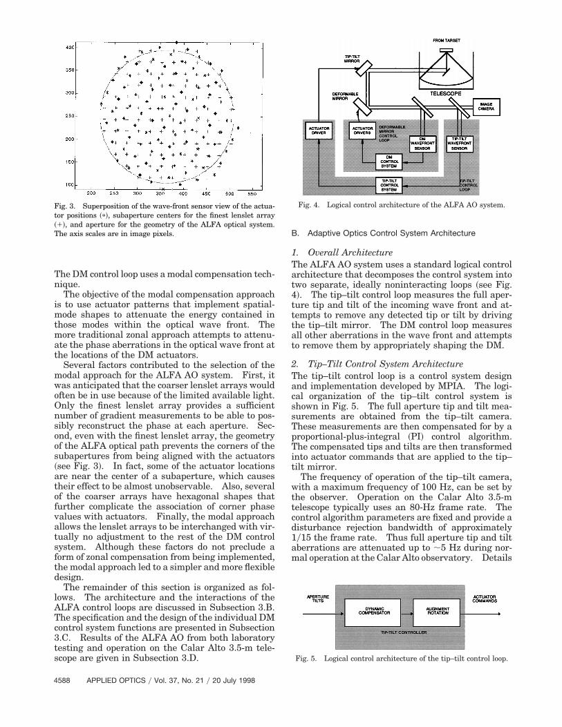
Several factors contributed to the selection of themodal approach for the ALFA AO system. First, itwas anticipated that the coarser lenslet arrays wouldoften be in use because of the limited available light.Only the finest lenslet array provides a sufficientnumber of gradient measurements to be able to pos-sibly reconstruct the phase at each aperture. Sec-ond, even with the finest lenslet array, the geometryof the ALFA optical path prevents the corners of thesubapertures from being aligned with the actuators~see Fig. 3!. In fact, some of the actuator locationsare near the center of a subaperture, which causestheir effect to be almost unobservable. Also, severalof the coarser arrays have hexagonal shapes thatfurther complicate the association of corner phasevalues with actuators. Finally, the modal approachallows the lenslet arrays to be interchanged with vir-tually no adjustment to the rest of the DM controlsystem. Although these factors do not preclude aform of zonal compensation from being implemented,the modal approach led to a simpler and more flexibledesign.
The remainder of this section is organized as fol-lows. The architecture and the interactions of theALFA control loops are discussed in Subsection 3.B.The specification and the design of the individual DMcontrol system functions are presented in Subsection3.C. Results of the ALFA AO from both laboratorytesting and operation on the Calar Alto 3.5-m tele-scope are given in Subsection 3.D.
Fig. 3. Superposition of the wave-front sensor view of the actua-tor positions ~p!, subaperture centers for the finest lenslet array~1!, and aperture for the geometry of the ALFA optical system.The axis scales are in image pixels.
4588 APPLIED OPTICS y Vol. 37, No. 21 y 20 July 1998
B. Adaptive Optics Control System Architecture
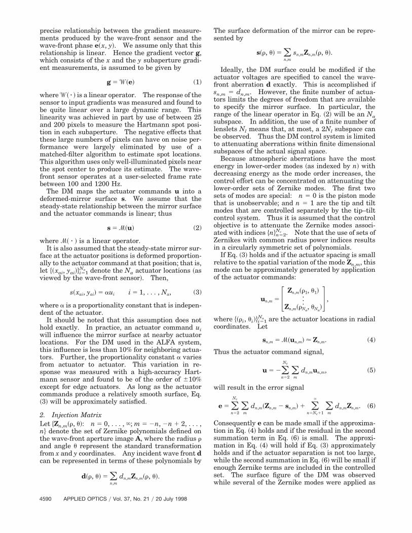
1. Overall ArchitectureThe ALFA AO system uses a standard logical controlarchitecture that decomposes the control system intotwo separate, ideally noninteracting loops ~see Fig.4!. The tip–tilt control loop measures the full aper-ture tip and tilt of the incoming wave front and at-tempts to remove any detected tip or tilt by drivingthe tip–tilt mirror. The DM control loop measuresall other aberrations in the wave front and attemptsto remove them by appropriately shaping the DM.
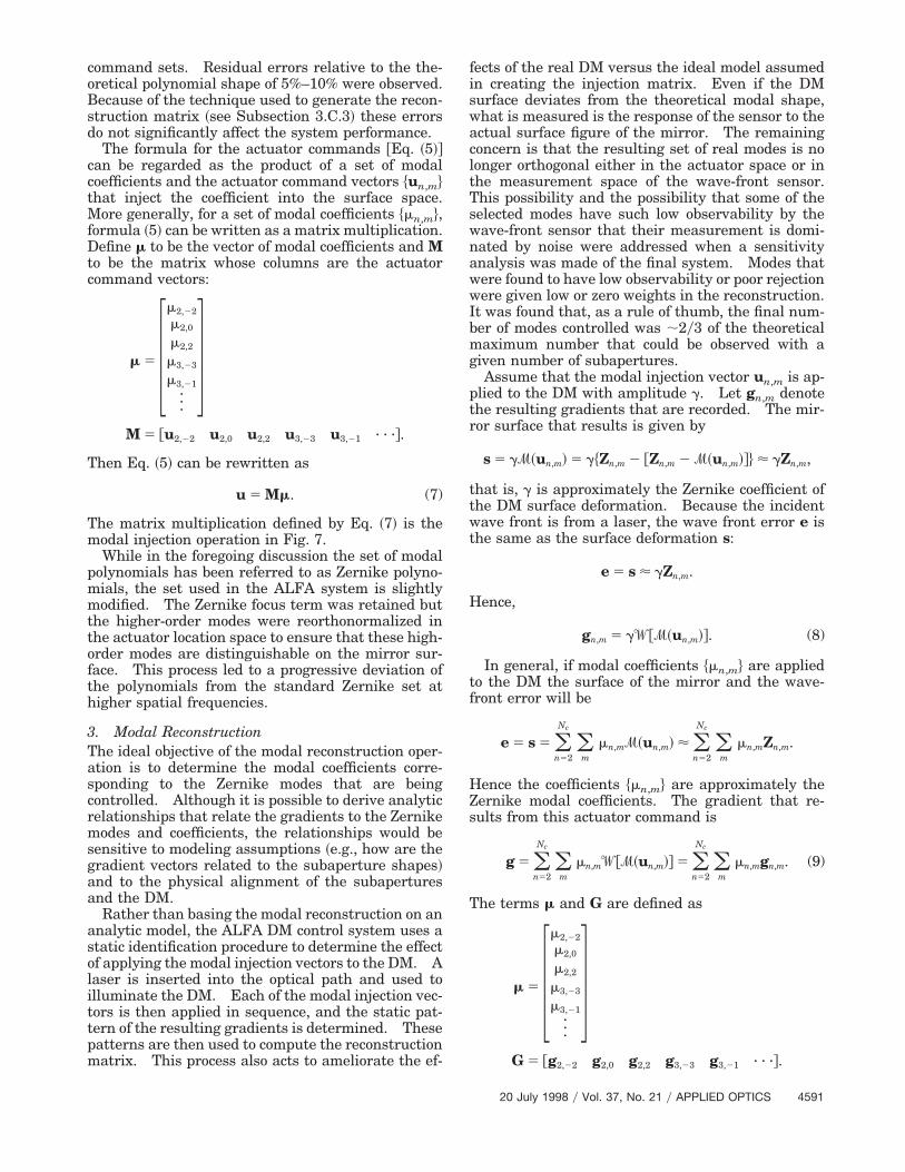
2. Tip–Tilt Control System ArchitectureThe tip–tilt control loop is a control system designand implementation developed by MPIA. The logi-cal organization of the tip–tilt control system isshown in Fig. 5. The full aperture tip and tilt mea-surements are obtained from the tip–tilt camera.These measurements are then compensated for by aproportional-plus-integral ~PI! control algorithm.The compensated tips and tilts are then transformedinto actuator commands that are applied to the tip–tilt mirror.
The frequency of operation of the tip–tilt camera,with a maximum frequency of 100 Hz, can be set bythe observer. Operation on the Calar Alto 3.5-mtelescope typically uses an 80-Hz frame rate. Thecontrol algorithm parameters are fixed and provide adisturbance rejection bandwidth of approximately1y15 the frame rate. Thus full aperture tip and tiltaberrations are attenuated up to ;5 Hz during nor-mal operation at the Calar Alto observatory. Details
Fig. 4. Logical control architecture of the ALFA AO system.
Fig. 5. Logical control architecture of the tip–tilt control loop.
of the design and operation of the tip–tilt control loopcan be found in Ref. 4.
In an alternative configuration the tip–tilt signalsare derived from the wave-front sensor data and thusare available at the same frame rate as the higher-order wave-front estimations. This mode is usablefor only natural guide-star operation because the la-ser guide star does not yield valid tilt information.
3. Deformable Mirror Control System ArchitectureThe logical control architecture of the DM controlsystem is shown in Fig. 6. The subaperture gradi-ents are local gradients of the phase of the incomingwave front, as measured by the Hartmann sensor.Given a set of spatial modes to be compensated for,the modal reconstructor uses the subaperture gradi-ents to determine the coefficients of the modes thatare present in the wave front. These modal coeffi-cients can be adjusted by application of an offset.These offsets are available to allow for the compen-sation of known differences between the modal esti-mate and the true wave-front error. An example ofthis is the focus error due to the zenith distance de-pendence of the range to the sodium layer. In thatcase an open-loop focus offset calculated from thezenith angle is applied to prevent drift in the imagefocus for stellar objects. The dynamic compensationof the modal coefficients is designed to attenuate eachof the modes that is being compensated for. Thecompensated modal coefficients are then multipliedby the modal injector to generate actuator commandsthat will produce the corresponding modal pattern onthe surface of the DM.
The logical architecture of the more standard zonalapproach to AO design is virtually identical to thatshown in Fig. 6. In the zonal approach, the recon-structor attempts to compute the phase of the wavefront at the actuator locations. Each local phase isthen compensated for, and the compensated phase isused directly to drive the actuators. The only mod-ification required to the architecture of Fig. 6 is thatthe modal injection function become an identity ~i.e.,a direct feedthrough of the compensated phases to the
Fig. 6. Logical control architecture of the DM control system.
actuator drives!. In fact, the zonal approach can beregarded as a special case of the modal approach inwhich the modes to be compensated for are spatialpoint functions at the actuator locations.
C. Design of the Deformable-Mirror Control SystemFunction
1. Modal Approach to the Deformable-MirrorControl ProblemFigure 7 contains a block diagram representation ofthe principal elements of the DM feedback loop of theALFA AO system. The principal components of thesystem are the DM, the wave-front sensor, the modalreconstructor, the dynamic modal compensation sys-tem, and the modal injection system. The functionof the block that represents the DM in the feedbackloop is to map the applied controls into a modifiedmirror surface s. The incident wave front ~includingthe atmosphere-induced aberration d! is reflected offthe surface to produce the reflected wave front e.The phase of the reflected wave front is the sum of thephase variation induced by atmospheric aberrationsof the incident wave front d and the phase variationinduced by the deformed mirror surface. Thus theatmospheric wave-front aberrations are representedas additive disturbances.
Physically, the wave-front aberrations d, the effectof the deformed mirror surface s, and the reflectedwave front e are distributed signals with continuousspatial and temporal variations. As viewed by thewave-front sensor, these signals are denoted by d~x,y!, s~x, y!, and e~x, y!, respectively, where the z axisis taken to be along the optical path and the x axisand the y axis define the viewing plane of the sensor.The relationship between these signals is
e~x, y! 5 s~x, y! 1 d~x, y!.
It is assumed that each of the signals belongs to aHilbert ~inner product! space * of functions definedon the aperture disk A as viewed by the wave-frontsensor, with an inner product
^a, b& 5 *A
a~x, y!b~x, y!dxdy.
The resulting wave-front error vector e~x, y! ismeasured by the wave-front sensor. The wave-frontsensor measures an approximation to the average xand y slopes of the phase over the subaperture. Forthe purposes of designing the DM control systemfunctions, it will not be necessary to determine the
Fig. 7. Block diagram of thefeedback loop of the DM. DyA,digital–analog converter.
20 July 1998 y Vol. 37, No. 21 y APPLIED OPTICS 4589
precise relationship between the gradient measure-ments produced by the wave-front sensor and thewave-front phase e~x, y!. We assume only that thisrelationship is linear. Hence the gradient vector g,which consists of the x and the y subaperture gradi-ent measurements, is assumed to be given by
g 5 0~e! (1)
where 0~ z ! is a linear operator. The response of thesensor to input gradients was measured and found tobe quite linear over a large dynamic range. Thislinearity was achieved in part by use of between 25and 200 pixels to measure the Hartmann spot posi-tion in each subaperture. The negative effects thatthese large numbers of pixels can have on noise per-formance were largely eliminated by use of amatched-filter algorithm to estimate spot locations.This algorithm uses only well-illuminated pixels nearthe spot center to produce its estimate. The wave-front sensor operates at a user-selected frame ratebetween 100 and 1200 Hz.
The DM maps the actuator commands u into adeformed-mirror surface s. We assume that thesteady-state relationship between the mirror surfaceand the actuator commands is linear; thus
s 5 }~u! (2)
where }~ z ! is a linear operator.It is also assumed that the steady-state mirror sur-
face at the actuator positions is deformed proportion-ally to the actuator command at that position; that is,let $~xai, yai!%i51
Na denote the Na actuator locations ~asviewed by the wave-front sensor!. Then,
s~xai, yai! 5 aui i 5 1, . . . , Na, (3)
where a is a proportionality constant that is indepen-dent of the actuator.
It should be noted that this assumption does nothold exactly. In practice, an actuator command uiwill influence the mirror surface at nearby actuatorlocations. For the DM used in the ALFA system,this influence is less than 10% for neighboring actua-tors. Further, the proportionality constant a variesfrom actuator to actuator. This variation in re-sponse was measured with a high-accuracy Hart-mann sensor and found to be of the order of 610%except for edge actuators. As long as the actuatorcommands produce a relatively smooth surface, Eq.~3! will be approximately satisfied.
2. Injection MatrixLet $Zn,m~r, u!: n 5 0, . . . , `; m 5 2n, 2n 1 2, . . . ,n% denote the set of Zernike polynomials defined onthe wave-front aperture image A, where the radius rand angle u represent the standard transformationfrom x and y coordinates. Any incident wave front dcan be represented in terms of these polynomials by
d~r, u! 5 dn,mZn,m~r, u!.
(n,m
4590 APPLIED OPTICS y Vol. 37, No. 21 y 20 July 1998
The surface deformation of the mirror can be repre-sented by
s~r, u! 5 (n,m
sn,mZn,m~r, u!.
Ideally, the DM surface could be modified if theactuator voltages are specified to cancel the wave-front aberration d exactly. This is accomplished ifsn,m 5 dn,m. However, the finite number of actua-tors limits the degrees of freedom that are availableto specify the mirror surface. In particular, therange of the linear operator in Eq. ~2! will be an Nasubspace. In addition, the use of a finite number oflenslets Nl means that, at most, a 2Nl subspace canbe observed. Thus the DM control system is limitedto attenuating aberrations within finite dimensionalsubspaces of the actual signal space.
Because atmospheric aberrations have the mostenergy in lower-order modes ~as indexed by n! withdecreasing energy as the mode order increases, thecontrol effort can be concentrated on attenuating thelower-order sets of Zernike modes. The first twosets of modes are special: n 5 0 is the piston modethat is unobservable; and n 5 1 are the tip and tiltmodes that are controlled separately by the tip–tiltcontrol system. Thus it is assumed that the controlobjective is to attenuate the Zernike modes associ-ated with indices $n%n52
Nc . Note that the use of sets ofZernikes with common radius power indices resultsin a circularly symmetric set of polynomials.
If Eq. ~3! holds and if the actuator spacing is smallrelative to the spatial variation of the mode Zn,m, thismode can be approximately generated by applicationof the actuator commands:
un,m 5 F Zn,m~r1, u1!···Zn,m~rNa
, uNa!G ,
where $~ri, ui!%i51Na are the actuator locations in radial
coordinates. Let
sn,m 5 }~un,m! < Zn,m. (4)
Thus the actuator command signal,
u 5 2(n52
Nc
(m
dn,mun,m, (5)
will result in the error signal
e 5 (n52
Nc
(m
dn,m~Zn,m 2 sn,m! 1 (n5Nc11
`
(m
dn,mZn,m. (6)
Consequently e can be made small if the approxima-tion in Eq. ~4! holds and if the residual in the secondsummation term in Eq. ~6! is small. The approxi-mation in Eq. ~4! will hold if Eq. ~3! approximatelyholds and if the actuator separation is not too large,while the second summation in Eq. ~6! will be small ifenough Zernike terms are included in the controlledset. The surface figure of the DM was observedwhile several of the Zernike modes were applied as
command sets. Residual errors relative to the the-oretical polynomial shape of 5%–10% were observed.Because of the technique used to generate the recon-struction matrix ~see Subsection 3.C.3! these errorsdo not significantly affect the system performance.
The formula for the actuator commands @Eq. ~5!#can be regarded as the product of a set of modalcoefficients and the actuator command vectors $un,m%that inject the coefficient into the surface space.More generally, for a set of modal coefficients $mn,m%,formula ~5! can be written as a matrix multiplication.Define m to be the vector of modal coefficients and Mto be the matrix whose columns are the actuatorcommand vectors:
m 5 3m2,22
m2,0
m2,2
m3,23
m3,21···
4M 5 @u2,22 u2,0 u2,2 u3,23 u3,21 · · ·#.
Then Eq. ~5! can be rewritten as
u 5 Mm. (7)
The matrix multiplication defined by Eq. ~7! is themodal injection operation in Fig. 7.
While in the foregoing discussion the set of modalpolynomials has been referred to as Zernike polyno-mials, the set used in the ALFA system is slightlymodified. The Zernike focus term was retained butthe higher-order modes were reorthonormalized inthe actuator location space to ensure that these high-order modes are distinguishable on the mirror sur-face. This process led to a progressive deviation ofthe polynomials from the standard Zernike set athigher spatial frequencies.
3. Modal ReconstructionThe ideal objective of the modal reconstruction oper-ation is to determine the modal coefficients corre-sponding to the Zernike modes that are beingcontrolled. Although it is possible to derive analyticrelationships that relate the gradients to the Zernikemodes and coefficients, the relationships would besensitive to modeling assumptions ~e.g., how are thegradient vectors related to the subaperture shapes!and to the physical alignment of the subaperturesand the DM.
Rather than basing the modal reconstruction on ananalytic model, the ALFA DM control system uses astatic identification procedure to determine the effectof applying the modal injection vectors to the DM. Alaser is inserted into the optical path and used toilluminate the DM. Each of the modal injection vec-tors is then applied in sequence, and the static pat-tern of the resulting gradients is determined. Thesepatterns are then used to compute the reconstructionmatrix. This process also acts to ameliorate the ef-
fects of the real DM versus the ideal model assumedin creating the injection matrix. Even if the DMsurface deviates from the theoretical modal shape,what is measured is the response of the sensor to theactual surface figure of the mirror. The remainingconcern is that the resulting set of real modes is nolonger orthogonal either in the actuator space or inthe measurement space of the wave-front sensor.This possibility and the possibility that some of theselected modes have such low observability by thewave-front sensor that their measurement is domi-nated by noise were addressed when a sensitivityanalysis was made of the final system. Modes thatwere found to have low observability or poor rejectionwere given low or zero weights in the reconstruction.It was found that, as a rule of thumb, the final num-ber of modes controlled was ;2y3 of the theoreticalmaximum number that could be observed with agiven number of subapertures.
Assume that the modal injection vector un,m is ap-plied to the DM with amplitude g. Let gn,m denotethe resulting gradients that are recorded. The mir-ror surface that results is given by
that is, g is approximately the Zernike coefficient ofthe DM surface deformation. Because the incidentwave front is from a laser, the wave front error e isthe same as the surface deformation s:
e 5 s < gZn,m.
Hence,
gn,m 5 g0@}~un,m!#. (8)
In general, if modal coefficients $mn,m% are appliedto the DM the surface of the mirror and the wave-front error will be
e 5 s 5 (n52
Nc
(m
mn,m}~un,m! < (n52
Nc
(m
mn,mZn,m.
Hence the coefficients $mn,m% are approximately theZernike modal coefficients. The gradient that re-sults from this actuator command is
g 5 (n52
Nc
(m
mn,m0@}~un,m!# 5 (n52
Nc
(m
mn,mgn,m. (9)
The terms m and G are defined as
m 5 3m2,22
m2,0
m2,2
m3,23
m3,21···
4G 5 @g2,22 g2,0 g2,2 g3,23 g3,21 · · ·#.
20 July 1998 y Vol. 37, No. 21 y APPLIED OPTICS 4591
Fig. 8. Mapping from compen-sated modes to reconstructedmodes.
Then Eq. ~9! can be rewritten as
g 5 Gm. (10)
The matrix G is left invertible if the modes that are tobe controlled can be observed independently by thewave-front sensor. Assuming this is the case, themodal coefficients can be determined ~reconstructed!by
m 5 ~GTG!21Gg ; Hg, (11)
where H is the modal reconstruction matrix.The ALFA DM control system incorporates the on-
line calibration of the modal reconstruction matrixdescribed in the preceding paragraphs. Specifically,the on-line calibration applies actuator commandscorresponding to a constant modal injection vectorun,m. After any transients have died out, the gradi-ent vector is averaged over 20 frames to obtain gn,m.The process is repeated for each mode to be con-trolled. The matrix G is constructed, and the recon-struction matrix H is computed. The identificationprocess takes less than 2 min for 20 modes.
4. Compensation AlgorithmDynamic Models. Design of the compensation algo-rithm requires models of the significant dynamics ofthe control loop. Until this point, the models thatwere developed for the elements of the control loopwere static mappings that determined steady-staterelationships between their inputs and outputs.There are three significant sources of dynamic vari-ations in the DM control loop that must be represent-ed.6 First, the DM actuators exhibit first-orderdynamic responses at frequencies of interest to theAO problem. Second, the computation time re-quired for reading the CCD, constructing the gradi-ents, and computing the modal coefficients can besignificant. Finally, the inherent time discretiza-tion induced by the frame rate of the wave-front sen-sor camera requires that the system be treated as asampled-data system. Hence the dynamics of thedigital–analog ~DyA! converter and sampling processare important.
A block diagram of the mapping from the output ofthe compensator algorithm ~the commanded modesmm! to the input to the compensator algorithm ~thereconstructed modes m! is shown in Fig. 8. Themodal injection function contains no dynamics and issimply a matrix multiplication. The DM has first-order dynamics associated with the actuators ~seediscussion in Ref. 5! as well as the mapping into thesurface deformation defined by Eq. ~2!. We modelthe actuator dynamics as identical for each actuator.Thus the DM can be decomposed as shown in Fig. 9.
4592 APPLIED OPTICS y Vol. 37, No. 21 y 20 July 1998
From the manufacturer specifications and laboratorymeasurements, the time constant of the DM actua-tors ta was determined to be ta 5 2 3 1024 s.
The wave-front sensor can be modeled as threeseparate functions ~see Fig. 10!: the static mappingbetween the wave-front error e and the gradientsgiven by Eq. ~1!, the sampling of the wave front dueto the camera frame rate, and the time delay due tothe computation of the gradients and the recon-structed modes. Note that the last element could bebroken into the two separate delays associated withthe gradient computation and camera readout andthe modal reconstruction. Because the effects ofthese delays are identical as far as the compensationalgorithm is concerned, they are treated as one.
As discussed in Ref. 6 it is reasonable to assumethat the wave-front sensor–reconstructor delays areidentical in all channels. Based on a timing dia-gram of the computations and the laboratory mea-surements, the effective delay tc was found to be tc 51.5 3 1023 s. Because the computation time asso-ciated with the modal reconstruction was included inthe wave-front sensor, the modal reconstruction isrepresented as the matrix multiplication given by Eq.~11!.
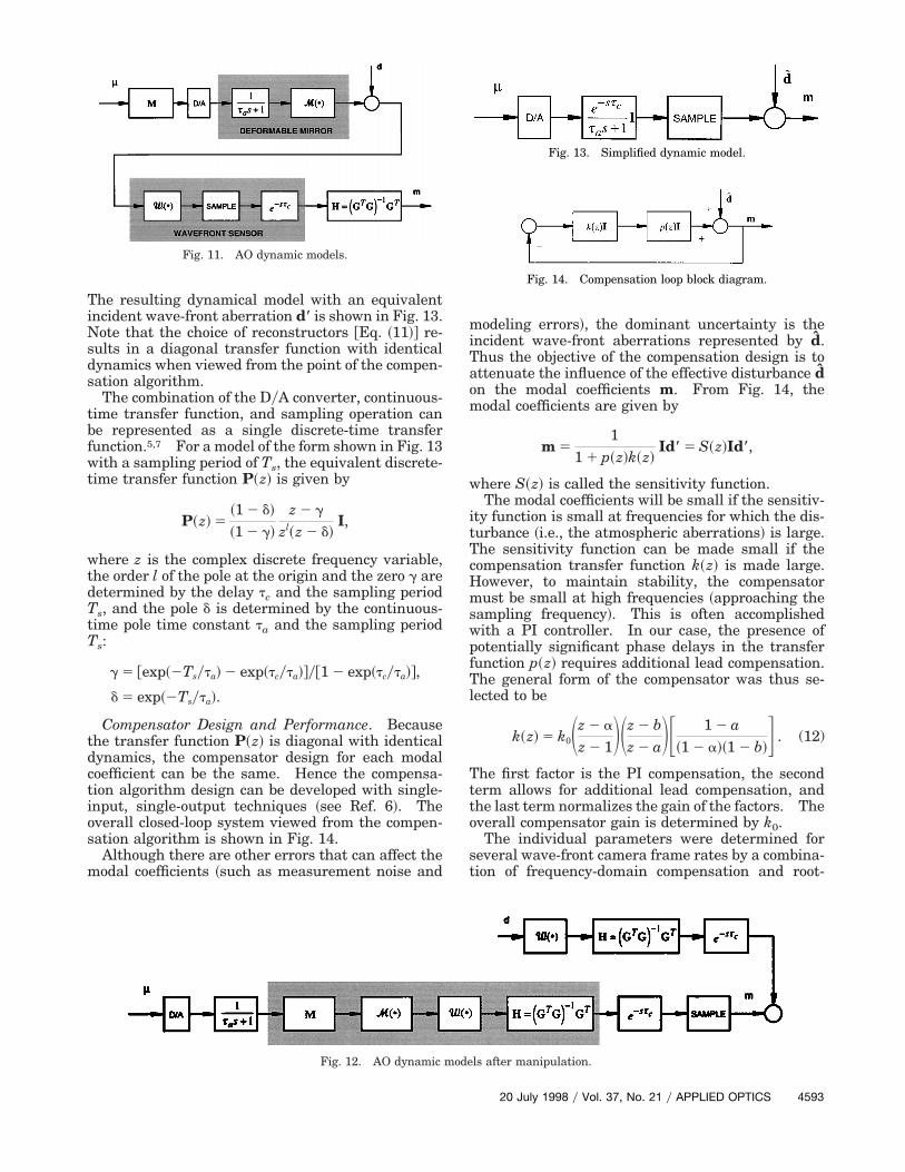
The overall block diagram, including the signifi-cant dynamic effects, is shown in Fig. 11. We cansimplify this model by noting that the DyA operationand the modal injection matrix multiplications can be~for the purpose of mathematical modeling! inter-changed. Similarly, the sampling operation, themodal reconstruction, and the delay can be inter-changed. The addition of incident wave-front signalcan be moved by block diagram manipulation to theend of the blocks ~see Fig. 12!. Finally, the staticDM function, the static wave-front sensing function,and the modal reconstruction can be combined byEqs. ~8!, ~10!, and ~11!:
H~0 z }!M 5 I.
Fig. 9. Dynamic model of the DM.
Fig. 10. Dynamic model of the wave-front sensor.
The resulting dynamical model with an equivalentincident wave-front aberration d* is shown in Fig. 13.Note that the choice of reconstructors @Eq. ~11!# re-sults in a diagonal transfer function with identicaldynamics when viewed from the point of the compen-sation algorithm.
The combination of the DyA converter, continuous-time transfer function, and sampling operation canbe represented as a single discrete-time transferfunction.5,7 For a model of the form shown in Fig. 13with a sampling period of Ts, the equivalent discrete-time transfer function P~z! is given by
P~z! 5~1 2 d!
~1 2 g!
z 2 g
zl~z 2 d!I,
where z is the complex discrete frequency variable,the order l of the pole at the origin and the zero g aredetermined by the delay tc and the sampling periodTs, and the pole d is determined by the continuous-time pole time constant ta and the sampling periodTs:
g 5 @exp~2Tsyta! 2 exp~tcyta!#y@1 2 exp~tcyta!#,
d 5 exp~2Tsyta!.
Compensator Design and Performance. Becausethe transfer function P~z! is diagonal with identicaldynamics, the compensator design for each modalcoefficient can be the same. Hence the compensa-tion algorithm design can be developed with single-input, single-output techniques ~see Ref. 6!. Theoverall closed-loop system viewed from the compen-sation algorithm is shown in Fig. 14.
Although there are other errors that can affect themodal coefficients ~such as measurement noise and
Fig. 11. AO dynamic models.
modeling errors!, the dominant uncertainty is theincident wave-front aberrations represented by d.Thus the objective of the compensation design is toattenuate the influence of the effective disturbance don the modal coefficients m. From Fig. 14, themodal coefficients are given by
m 51
1 1 p~z!k~z!Id* 5 S~z!Id*,
where S~z! is called the sensitivity function.The modal coefficients will be small if the sensitiv-
ity function is small at frequencies for which the dis-turbance ~i.e., the atmospheric aberrations! is large.The sensitivity function can be made small if thecompensation transfer function k~z! is made large.However, to maintain stability, the compensatormust be small at high frequencies ~approaching thesampling frequency!. This is often accomplishedwith a PI controller. In our case, the presence ofpotentially significant phase delays in the transferfunction p~z! requires additional lead compensation.The general form of the compensator was thus se-lected to be
k~z! 5 k0Sz 2 a
z 2 1DSz 2 bz 2 aDF 1 2 a
~1 2 a!~1 2 b!G . (12)
The first factor is the PI compensation, the secondterm allows for additional lead compensation, andthe last term normalizes the gain of the factors. Theoverall compensator gain is determined by k0.
The individual parameters were determined forseveral wave-front camera frame rates by a combina-tion of frequency-domain compensation and root-
Fig. 13. Simplified dynamic model.
Fig. 14. Compensation loop block diagram.
Fig. 12. AO dynamic models after manipulation.
20 July 1998 y Vol. 37, No. 21 y APPLIED OPTICS 4593
locus methods. The parameters for each of theframe rates considered are shown in Table 2. Bodeplots of the magnitudes of the sensitivity function areshown in Fig. 15 for the frame rates of 300 and 1200Hz. Note that the disturbance rejection bandwidthin each case is approximately 1y12 of the frame rate~in hertz! and that the sensitivity peak in each case isapproximately 6 dB. Also, the design parametersfor all designs below 600 Hz are identical because thephase lags from the actuator dynamics and compu-tations are almost insignificant at those frequencies.The additional lead compensation term in Eq. ~12! isneeded for only the 900- and 1200-Hz designs.
D. Results
The ALFA AO system was installed on the 3.5-m tele-scope at the Calar Alto Observatory in Spain in Sep-tember, 1996. Stable operation of the AO loops wasachieved from the beginning. A small selection of re-cent results are presented here. For the latest infor-mation please refer to the ALFA site on the Internet atwww.mpia-hd.mpg.deyMPIAyProjectsyALFA.
Several stars in the 4–6 magnitude range wereobserved with wave-front camera frame rates up to
Fig. 15. Magnitudes of the sensitivity function for 300- and1200-Hz designs.
Table 2. Compensation Parameters and Disturbance RejectionBandwidths for Various Wave-Front Sensor Camera Frame Rates
4594 APPLIED OPTICS y Vol. 37, No. 21 y 20 July 1998
900 Hz with the parameters from Table 2 and thetip–tilt loop operating at an 80-Hz frame rate. Theresults from observations of 14 Peg and f Ursa Majoris with the MPIA MAGIC infrared camera system areshown in Fig. 16. The use of ALFA resulted in sig-nificant increases in the peak intensity with a corre-sponding increase in the Strehl ratio.
The ultimate goal for the ALFA system is the use ofthe sodium layer guide star as the source for thecontrol system. In an observing run in early Decem-ber, closed-loop operation was first achieved with thelaser source. The laser guide star has an equivalentbrightness of a 10 magnitude star. ALFA providedstable correction at a 60-Hz frame rate with usefulimprovement in image quality. Performance withthe laser source is chiefly limited by the detectornoise of ;10 electronsypixel. A full analysis of thesystem performance relative to theory and model pre-dictions is still in progress. Some preliminary re-sults pertaining to the control-loop performance arepresented below.
Figure 17 shows the magnitudes of the open-loopand the closed-loop spectra of the focus mode com-puted from 20-s data segments ~6000 frames!. Asexpected, there is significant attenuation of the dis-turbance below 10 Hz. Figure 18 shows the transferfunction computed from the spectra shown in Fig. 17and compares them with the theoretical closed-looptransfer function ~see also Fig. 15!.
4. Real-Time Modal Control Processor
A. Hardware Implementation Algorithm
In many AO systems, a single-matrix multiply is usedto convert wave-front slopes to actuator control sig-nals.8,9 As discussed in detail in Section 3, in orderto accommodate the varied requirements, we chose todivide the wave-front reconstruction into two parts.A schematic for the wave-front control is shown inFig. 6.
The wave front is first reconstructed and then pro-jected into Zernike modes in the box marked ModalReconstructor. The Modal Offsets junction appliesboth an additive offset and a weighted filtering func-tion to the reconstruction. These modal weights canbe computed off line and can be changed at any time.Another matrix multiply is performed in the ModalInjection box in order to convert the filtered modesinto actuator commands for the DM.
1. Hardware ImplementationAll matrix operations are implemented in the RTC byfive digital signal processor ~DSP! boards, with eachboard containing four DSP chips, thus making a totalof 20 DSP processors in which to distribute all re-quired calculations. The DSP chips are allocated toeach operation according to Table 3.
This implementation is capable of projecting 50wave-front control modes in 833-ms execution time.The mathematical operations for this processor arecapable of being scaled to 349 actuators by the addi-tion of more DSP boards. A photograph of the RTC
Fig. 16. Top pair: open loop ~left! and closed loop ~right! images obtained at a wavelength of 2.2 mm of the 0.24-arc min binary f UrsaMajoris ~HR 3894, mv 5 4.6!. Observation was made through clouds in 1.7 arc min seeing on 1 March 1997. The AO system operatedat a 900-Hz frame rate and corrected 20 modes. The data represent the sum of several exposures for a total exposure time of 50 s. Thetwo components of the binary are clearly resolved. Bottom pair: open loop ~left! and closed loop ~right! images obtained at a wavelengthof 2.2 mm of the star 14Peg ~mv 5 5.04! obtained on 21 July 1997. For the data 17 modes were corrected at a loop frequency of 100 Hz.The Strehl ratio improved from 2.4% open loop to 20% closed loop. The seeing was 0.85 arc min. The data represent the sum of 100exposures at 0.2 s. No image restoration techniques have been applied to these data.
is shown in Fig. 19. The DSP boards are housed ina VME-based card cage. The five boards share databy means of the connecting cables in the front. Thetwo boards at the left are for external communica-tions.
2. Software ConsiderationsThe RTC has been programmed to interact with theentire AO system both in real-time and for off-linestudies. In real time the RTC performs its wave-front control function, and off line it provides wave-front information for atmospheric studies and todetermine, for example, an optimal set of weights formodal control. In real time, the RTC is programmed
in C and takes instructions from a Motorola 68060running the real-time VxWorks operating system.10
For off-line studies the RTC takes instructions re-layed by EPICS ~Experimental Physics IndustrialControl System11!, a client–server model distributeddatabase. EPICS has the ability to communicatebetween VxWorks and our host computers. The toplayer of control between the RTC and the rest of theAO system is shown in Fig. 20. The RTC is con-tained within the ellipse marked AO Loop.
Figure 21 shows how off-line queries are handledby the RTC. A data manager sends requests to thereal-time interface, which then returns the requesteddata. This information is input into WAVELAB,
20 July 1998 y Vol. 37, No. 21 y APPLIED OPTICS 4595
AOA’s commercially available software package forShack–Hartmann data analysis. WAVELAB con-tains a library of C language routines, all of which canbe called on a command line or embedded into a script
Fig. 17. Spectra of focus-mode coefficients with the AO loop openand closed.
Fig. 18. Transfer function computed from observed data.
Fig. 19. Wave-front control processor box at lower left, along withone of the authors ~JN!.
4596 APPLIED OPTICS y Vol. 37, No. 21 y 20 July 1998
by means of the Tcl language. Both Tcl and itsgraphic language, Tk,12 are used to write specializeddata analysis procedures for analyzing atmosphericdata. The results of these analyses are then sentback through the data manager and the real-timeinterface so that weights can be modified in the RTC.
5. Summary
A flexible wave-front control processor was built andintegrated by AOA for a sodium laser guide-star AOsystem to be located on a 3.6-m telescope located inCalar Alto, Spain, and operated by the MPIA, Hei-delberg. The processor was built in response to re-quirements for an AO system that would need tooperate under varied conditions and could be up-
Fig. 20. Top level of software control between the RTC and theentire AO system. GUI, graphic user interface; LGS, laser guidestar; TCS, telescope control system.
Fig. 21. Data flow diagram for obtaining off-line data from thewave-front control processor.
Table 3. Allocation of Wave-Front Control Functions in a DSP-BasedProcessor
Number of DSP’s Operation
5 Camera input, gain, offset8 Gradients ~two algorithms!4 Reconstructionymodal projection1 Compensation ~weighting!2 Modal injectionyDM output
graded at a modest cost. The processor can be usedto perform modal wave-front control by a two-matrix-multiply approach and has the ability to accommo-date varying wave-front sensor geometry, systembandwidths, and atmospheric weights. This proces-sor was built from commercial DSP boards. Its soft-ware is written to interact with both real-time andoff-line requests and makes use of widely supportedcommercial and public domain software tools.
The authors acknowledge the help of the whole ofTeam ALFA, both at AOA and at MPIA. The re-search reported here was funded by MPIA and by theU.S. National Science Foundation contract ECS-95-10449.
References and Notes1. J. Beckers, “Adaptive optics for astronomy: principles, per-
formance, and applications,” Annu. Rev. Astron. Astrophys.31, 13–62 ~1993!.
2. A. Wirth, F. Landers, B. Trvalik, J. Navetta, and T. Bruno, “Alaser guide star atmospheric compensation system for the 3.5mCalar Alto telescope,” in Adaptive Optics, Vol. 23 of 1995 OSATechnical Digest Series ~Optical Society of America, Washing-ton, D.C., 1995!, paper MA3-1.
3. R. J. Noll, “Zernike polynomials and atmospheric turbulence,”J. Opt. Soc. Am. 66, 207–211 ~1976!.
4. J. Y. Wang and D. E. Silva, “Wave-front interpretation withZernike polynomials,” Appl. Opt. 19, 1510–1518 ~1980!.
5. A. Glindemann, M. J. McCaughran, S. Hippler, C. Wagner,
and R.-R. Rohloff, “CHARM: a tipytilt tertiary system for theCalar Alto 3.5m telescope,” presented at the OSA summertopical meeting on Adaptive Optics, Maui, 8–12 July 1996.
6. J. Huang, D. P. Looze, N. Denis, D. Castanon, and A. Wirth,“Modeling and identification of adaptive optics systems,” Int. J.Control (to be published).
7. G. F. Franklin, J. D. Powell, and A. Emami-Naeini, FeedbackControl of Dynamic Systems ~Addison-Wesley, Reading, Mass.,1988!.
8. G. Rousset, J.-L. Beuzit, N. Hubin, E. Gendron, P.-Y. Madec, C.Boyer, J. P. Gaffard, J.-C. Richard, M. Vittot, P. Gigan, andP. J. Lena, “Performance and results of the COME-ON1 adap-tive optics system at the ESO 3.6m telescope,” in AdaptiveOptics in Astronomy, M. A. Ealey and F. Merkle, eds., Proc.SPIE 2201, 1088–1095 ~1994!.
9. J. L. Beuzit, N. Hubin, E. Gendron, L. Demailly, P. Gigan, F.Lacombe, F. Chazallet, D. Rabaud, and G. Rousset, “ADONIS:a user-friendly adaptive optics system for the ESO 3.6m tele-scope,” in Adaptive Optics, Vol. 23 of 1995 OSA TechnicalDigest Series ~Optical Society of America, Washington, D.C.,1995!, paper MC1-1.
10. VxWorks is a product of Wind River Systems, Inc., 1010 At-lantic Avenue, Alameda, Calif. 94501.
11. EPICS is free to nonprofit and government sites from LosAlamos National Laboratories and is commercially availablefrom Kinetic Systems Corp., 7308 South Alton Way, Bldg. 2,Engelwood, Colo. 80112.
12. Both Tcl and Tk are freely available in the public domain.For further information on these languages, see B. B. Welsh,Practical Programming in Tcl and Tk ~Prentice-Hall, UpperSaddle River, N.J., 1995!.
20 July 1998 y Vol. 37, No. 21 y APPLIED OPTICS 4597