Real Time Optimization in chemical processes: evaluation ... · I would like to express my special...

JOSÉ EDUARDO ALVES GRACIANO

Real Time Optimization in chemical processes: evaluation of

strategies, improvements and industrial application

São Paulo

2016




Tese apresentada à Escola Politécnica da

Universidade de São Paulo para obtenção

do título de Doutor em Engenharia

São Paulo

2016




Tese apresentada à Escola Politécnica da

Universidade de São Paulo para obtenção

do título de Doutor em Engenharia

Área de concentração: Engenharia

Química

Orientador: Prof. Dr. Galo Antonio Carrillo

Le Roux

São Paulo

2016

Catalogação-na-publicação

Graciano, José Eduardo Aves

Real Time Optimization in chemical processes: evaluation of strategies,

improvements and industrial application / J. E. A. Graciano -- versão corr. --

São Paulo, 2016.

160 p.

Tese (Doutorado) - Escola Politécnica da Universidade de São Paulo.

Departamento de Engenharia Química.

1.Otimização em tempo real 2.Controle de processos 3.Estimação de

parâmetros 4.self-optimizing control I.Universidade de São Paulo. Escola

Politécnica. Departamento de Engenharia Química II.t.

Este exemplar foi revisado e corrigido em relação à versão original, sob responsabilidade única do autor e com a anuência de seu orientador.

São Paulo, de de

Assinatura do autor:

Assinatura do orientador:

AGRADECIMENTOS

Ao professor Galo Antonio Carrillo Le Roux, pela oportunidade, orientação e

constante estímulo transmitido durante todo o trabalho.

I would like to express my special gratitude to Professor Lorenz T. Biegler for

receiving me in his research group, contributing to my professional and personal

development.

I sincerely thank Professor Johannes Jäschke for helping me in the development of

new ideas, which improved the quality of the present work.

Aos meus pais, Silvana e José, por todo carinho, dedicação e apoio incondicional às

minhas escolhas.

Às minhas irmãs Simone e Juliana, que sempre me inspiraram na busca pelo

conhecimento.

Às minhas sobrinhas Heloísa e Manuela, pelos ótimos fins de semana que

passamos juntos.

À minha companheira Flávia, por todo amor, paciência, incentivo e risadas, que

sempre me ajudaram a esquecer os pequenos problemas do dia-a-dia.

Ao amigo Lucas, por sempre afirmar que tudo daria certo, discordando dos meus

argumentos contrários.

Ao amigo Diego que contribuiu imensamente na elaboração deste trabalho,

tornando-se um modelo para meu desenvolvimento profissional.

Aos amigos Bruno, André e Zé pelas correções e sugestões de melhoria deste

trabalho, bem como pelo apoio na organização dos churrascos que animaram nosso

departamento.

Aos meus colegas de laboratório, pelo apoio e auxílio durante a execução do

trabalho, bem como nos momentos de descontração nos nossos cafés de fim de

tarde.

Ao CNPq e à Petrobras, pelo apoio financeiro.

E a todos que colaboraram direta ou indiretamente, na execução deste trabalho.

E mesmo que pareça tolo

E sem sentido

Eu ainda brigo por sonhos

Eu ainda brigo

(Herbert Vianna)

RESUMO

O aumento da concorrência motiva a indústria a implementar ferramentas que

melhorem a eficiência de seus processos. A automação é uma dessas ferramentas,

e o Real Time Optimization (RTO) ou Otimização em Tempo Real, é uma

metodologia de automação que considera aspectos econômicos e restrições de

processos e equipamentos para atualizar o controle do processo, de acordo com

preços de mercado e distúrbios. Basicamente, o RTO usa um modelo

fenomenológico em estado estacionário para predizer o comportamento do

processo, em seguida, otimiza uma função objetivo econômica sujeita a esse

modelo. Embora amplamente utilizado na indústria, não há ainda um consenso geral

sobre os benefícios da implementação do RTO, devido a algumas limitações

discutidas no presente trabalho: incompatibilidade estrutural entre planta e modelo,

problemas de identificabilidade e baixa frequência de atualização dos set points.

Algumas metodologias de RTO foram propostas na literatura para lidar com o

problema da incompatibilidade entre planta e modelo. No entanto, não há uma

comparação que avalie a abrangência e as limitações destas diversas abordagens

de RTO, sob diferentes aspectos. Por esta razão, o método clássico de RTO é

comparado com metodologias mais recentes, baseadas em derivadas (Modifier

Adaptation, Integrated System Optimization and Parameter estimation, and Sufficient

Conditions of Feasibility and Optimality), utilizando-se o método de Monte Carlo. Os

resultados desta comparação mostram que o método clássico de RTO é coerente,

desde que seja proporcionado um modelo suficientemente flexível para se

representar a topologia do processo, um método de estimação de parâmetros

apropriado para lidar com características de ruído de medição e um método para

melhorar a qualidade da informação da amostra. Já os problemas de

identificabilidade podem ser observados a cada iteração de RTO, quando o método

atualiza alguns parâmetros-chave do modelo, o que é causado principalmente pela

ausência de medidas e ruídos. Por esse motivo, quatro abordagens de estimação de

parâmetros (Discriminação Rotacional, Seleção Automática e Estimação de

Parâmetros, Reparametrização via Geometria Diferencial e o clássico Mínimos

Quadrados não-lineares) são avaliados em relação à sua capacidade de predição,

robustez e velocidade. Os resultados revelam que o método de Discriminação

Rotacional é o mais adequado para ser implementado em um ciclo de RTO, já que

requer menos informação a priori, é simples de ser implementado e evita o

sobreajuste observado no método de Mínimos Quadrados. A terceira desvantagem

associada ao RTO é a baixa frequência de atualização dos set points, o que

aumenta o período em que o processo opera em condições subotimas. Uma

alternativa para lidar com este problema é proposta no presente trabalho,

integrando-se o RTO e o Self-Optimizing Control (SOC) através de um novo

algoritmo de Model Predictive Control (MPC). Os resultados obtidos com a nova

abordagem demonstram que é possível reduzir o problema da baixa frequência de

atualização dos set points, melhorando o desempenho econômico do processo. Por

fim, os aspectos práticos da implementação do RTO são discutidos em um estudo

de caso industrial, que trata de um processo de destilação com bomba de calor,

localizado na Refinaria de Paulínia (REPLAN - Petrobras). Os resultados deste

estudo sugerem que os parâmetros do modelo são estimados com sucesso pelo

método de Discriminação Rotacional; que o RTO é capaz de aumentar o lucro do

processo em cerca de 3%, o equivalente a 2 milhões de dólares por ano; e que a

integração entre SOC e RTO pode ser uma alternativa interessante para o controle

deste processo de destilação.

Palavras-chave: Otimização em Tempo Real. Controle de Processos. Estimação de Parâmetros. Self-optimizing control.

ABSTRACT

The increasing economic competition drives the industry to implement tools that

improve their processes efficiencies. The process automation is one of these tools,

and the Real Time Optimization (RTO) is an automation methodology that considers

economic aspects to update the process control in accordance with market prices

and disturbances. Basically, RTO uses a steady-state phenomenological model to

predict the process behavior, and then, optimizes an economic objective function

subject to this model. Although largely implemented in industry, there is not a general

agreement about the benefits of implementing RTO due to some limitations

discussed in the present work: structural plant/model mismatch, identifiability issues

and low frequency of set points update. Some alternative RTO approaches have

been proposed in literature to handle the problem of structural plant/model mismatch.

However, there is not a sensible comparison evaluating the scope and limitations of

these RTO approaches under different aspects. For this reason, the classical two-

step method is compared to more recently derivative-based methods (Modifier

Adaptation, Integrated System Optimization and Parameter estimation, and Sufficient

Conditions of Feasibility and Optimality) using a Monte Carlo methodology. The

results of this comparison show that the classical RTO method is consistent,

providing a model flexible enough to represent the process topology, a parameter

estimation method appropriate to handle measurement noise characteristics and a

method to improve the sample information quality. At each iteration, the RTO

methodology updates some key parameter of the model, where it is possible to

observe identifiability issues caused by lack of measurements and measurement

noise, resulting in bad prediction ability. Therefore, four different parameter

estimation approaches (Rotational Discrimination, Automatic Selection and

Parameter estimation, Reparametrization via Differential Geometry and classical

nonlinear Least Square) are evaluated with respect to their prediction accuracy,

robustness and speed. The results show that the Rotational Discrimination method is

the most suitable to be implemented in a RTO framework, since it requires less a

priori information, it is simple to be implemented and avoid the overfitting caused by

the Least Square method. The third RTO drawback discussed in the present thesis is

the low frequency of set points update, this problem increases the period in which the

process operates at suboptimum conditions. An alternative to handle this problem is

proposed in this thesis, by integrating the classic RTO and Self-Optimizing control

(SOC) using a new Model Predictive Control strategy. The new approach

demonstrates that it is possible to reduce the problem of low frequency of set points

updates, improving the economic performance. Finally, the practical aspects of the

RTO implementation are carried out in an industrial case study, a Vapor

Recompression Distillation (VRD) process located in Paulínea refinery from

Petrobras. The conclusions of this study suggest that the model parameters are

successfully estimated by the Rotational Discrimination method; the RTO is able to

improve the process profit in about 3%, equivalent to 2 million dollars per year; and

the integration of SOC and RTO may be an interesting control alternative for the VRD

process.

Keywords: Real Time Optimization. Process Control. Parameter Estimation, Self-

Optimizing Control.

LIST OF ILLUSTRATIONS

Figure 1.1 – Functional process control hierarchy ..................................................... 22

Figure 1.2 – “Classical RTO” or Model Parameter Adaptation (MPA) ....................... 23

Figure 1.3 – Illustrative example of an RTO implementation under uncertainties; (A) economic objective function value with respect to RTO iterations; (B) economic objective function profile with respect to controlled variables (Temperature and flow rate Fb). ..................................................................................................................... 25

Figure 2.1 – Classical RTO structure ........................................................................ 31

Figure 2.2 - ISOPE structure ..................................................................................... 34

Figure 2.3 - MA structure ........................................................................................... 35

Figure 2.4 - SCFO structure ...................................................................................... 38

Figure 2.5. - Williams Otto reactor ............................................................................. 40

Figure 2.6 – Optimum profile with respect to disturbances ........................................ 42

Figure 2.7 – MC experiments using noise free measurements and perfect model: (A) MPA, (B) MA, (C) ISOPE and (D) SCFO ................................................................... 44

Figure 2.8 – MC experiments using noisy measurements (0.5%) and perfect model: (A) MPA (B) MA (C) ISOPE and (D) SCFO ............................................................... 46

Figure 2.9 – MC experiments using noise free measurements and approximate model: (A) MPA (B) MA (C) ISOPE and (D) SCFO ................................................... 47

Figure 2.10 – MC experiments using noisy measurements (0.5%) and approximate model: (A) MPA (B) MA (C) ISOPE and (D) SCFO ................................................... 49

Figure 2.11. - Comparison between MPA with approximate model and free measurement noise. (A) MPA without Dual approach; (B) MPA with Dual approach 51

Figure 2.12. - Derivative analysis: (A – C – E - G) angle distribution between true and predicted gradient; (B – D – F - H) Norm ratio distribution between true and predicted gradient ...................................................................................................... 53

Figure 3.1 - Main steps of the RDG method. ............................................................. 62

Figure 3.2 - Rotational discrimination algorithm. ....................................................... 66

Figure 3.3 - APS algorithm. ....................................................................................... 69

Figure 3.4 – Objective function values obtained for the calibration set ...................... 77

Figure 3.5 – Frequency distribution of the estimated parameters by each method and true parameter values (vertical line). Figure A, B, C, D and E represents the parameters k1, k2, k3, k4 and kMT, respectively. ..................................................... 78

Figure 3.6 – Objective function values obtained for the validation set ....................... 80

Figure 3.7 – Concentration profiles of B and P predicted by LSq (A), RD (B), RDG (C) and APS (D) methods. (--) True concentration profile ............................................... 81

Figure 3.8 – Objective function values obtained in second case study on calibration set, from 0 to 5 (A) and from 58 to 63 (B). ................................................................. 82

Figure 3.9 - Frequency distribution of the estimated parameters by each method and true parameter values (vertical line) – Case study 2. ................................................ 83

Figure 3.10 – Objective function values obtained in second case study on validation set. ............................................................................................................................ 84

Figure 3.11 - Concentration profiles of measured components predicted by LSq (A), RD (B), and APS (C) methods – Case study 2. ......................................................... 85

Figure 3.12 - Cross section histogram of BM’s concentration profile at time 0.5 hours .................................................................................................................................. 85

Figure 3.13 – Concentration profiles of B and P predicted by LSq (A), RD (B), RDG (C) and APS (D) methods. (--) Nominal concentration profile. Noise-free Case 1 ..... 87

Figure 3.14 – Concentration profiles of B and P predicted by LSq (A), RD (B), RDG (C) and APS (D) methods. (--) Nominal concentration profile. Noise with standard deviation twice larger than the one used in base Case 1 .......................................... 87

Figure 4.1 - Proposed framework for the implementation of SOC in the RTO ........... 96

Figure 4.2 – MPC with zone control and SOC ........................................................... 97

Figure 4.3 - Schematic representation of ammonia production process .................. 103

Figure 4.4 - Profit of ammonia plant with respect to disturbances (This surface would be the cost if there were no active set changes) ..................................................... 104

Figure 4.5 - Active set map for the disturbance region, ammonia production case study. ....................................................................................................................... 104

(Each color denotes a region where the active set does not change. The variable names within the regions denote the constraints that are active) ............................ 104

Figure 4.6 - Steady state analysis results: (A) “classic” MPC, (B) MPC with artificial SOC variables and (C) MPC with zone control and SOC targets ............................ 106

Figure 4.7 – BTX process schematic representation ............................................... 107

Figure 4.8 – Cost profile with respect to disturbances ............................................. 109

Figure 4.9 – Active set map ..................................................................................... 109

Figure 4.10 – Steady state analysis results: (A) “classic” MPC, (B) MPC with artificial SOC variables and (C) MPC with zone control and SOC targets ............................ 111

Figure 4.11 – Comparison of the profit obtained by each MPC approach ............... 113

Figure 4.12 – Constrained variables profile ............................................................. 113

Figure 4.13 – Manipulated variables ....................................................................... 114

Figure 5.1 - Schematic representation of the VRD process .................................... 118

Figure 5.2 - Measured efficiency against the product .CP CPP Q ............................... 120

Figure 5.3 - Comparison of predicted and measured power ................................... 120

Figure 5.4 - Historic data of the reboiler temperature profile ................................... 121

Figure 5.5 - Historic data of the cooler temperature profile ..................................... 122

Figure 5.6 - Feed stream characteristics ................................................................. 123

Figure 5.7 - Products characteristics ....................................................................... 123

Figure 5.8 - Temperature profile of VRD column after parameter estimation .......... 127

Figure 5.9 - Optimized temperature profile .............................................................. 132

Figure.B1 - Algorithms results for ideal conditions (A) RTO path using approximated model and (B) RTO path using perfect model ......................................................... 148

LIST OF TABLES

Table 2.1 - Experimental design ................................................................................ 42

Table 2.2. - Root mean square error for MC experiments using noise free measurements and perfect model ............................................................................. 44

Table 2.3. - Frequency of achieving less than 1% profit loss in the last 5 RTO iterations of each region. MC experiments using noise free measurements and perfect model ............................................................................................................. 45

Table 2.4. - Average profit loss for MC experiments using noise free measurements and perfect model ...................................................................................................... 45

Table 2.5. - Root mean square error for MC experiments using noisy measurements (0.5%) and perfect model .......................................................................................... 45

Table 2.6. - Frequency of achieving less than 1% of profit loss in the last 5 RTO iterations of each region. MC experiments using noisy measurements (0.5%) and perfect model ............................................................................................................. 45

Table 2.7. - Average profit loss for MC experiments using noisy measurements (0.5%) and perfect model .......................................................................................... 46

Table 2.8. - Root mean square error for MC experiments using noise free measurements and approximate model .................................................................... 48

Table 2.9. - Frequency of achieving less than 1% profit loss in the last 5 RTO iterations of each region. MC experiments using noise free measurements and approximate model .................................................................................................... 48

Table 2.10. - Average profit loss for MC experiments using noise free measurements and approximate model ............................................................................................. 48

Table 2.11. - Root mean square error for MC experiments using noisy measurements (0.5%) and approximate model ................................................................................. 49

Table 2.12. - Frequency of achieving less than 1% profit loss in the last 5 RTO iterations of each region. MC experiments using noisy measurements (0.5%) and approximate model .................................................................................................... 50

Table 2.13. - Average profit loss for MC experiments using noisy measurements (0.5%) and approximate model ................................................................................. 50

Table 3.1 – Values of the parameters for the three-phase reactor model ................. 72

Table 3.2 – Initial conditions for the computational experiments ............................... 72

Table 3.3 – Upper and lower bounds of the guess of model parameters. ................. 73

Table 3.4 - Upper and lower bounds of the guess of the nominal values for the RDG method. ..................................................................................................................... 74

Table 3.5. Nominal reference parameter values for Dow Chemical parameter estimation problem. ................................................................................................... 75

Table 3.6 - Initial conditions for the computational experiments for case study 2. ..... 76

Table 3.7 - Upper and Lower bounds for the parameters initial guess and optimization step for case study 2 ............................................................................. 76

Table 3.8 – Mean values of the parameters obtained in the MC analysis. ................ 78

Table 3.9 – Variance of the parameters obtained in the MC analysis ....................... 79

Table 3.10 – Parameter ranking (as percentage) according to the criteria used in the APS method. ............................................................................................................. 79

Table 3.11 – Objective function statistics in calibration and validation sets ............... 80

Table 3.12 - Parameter ranking (as percentage) according to the criteria used in the APS method – study case 2. ..................................................................................... 83

Table 4.1. - Set of controlled variables for each Case (AV: artificial variable) ......... 106

Table 4.2 – Parameters values ................................................................................ 108

Table 4.3 – Set of controlled variables for each experiment ................................... 110

Table 5.1 - Summary of the parameter estimation results for the WO case study... 126

Table 5.2 - Parameters used in the VRD estimation ............................................... 127

Table 5.3 - Summary of the parameter estimation results for the VRD process case study ........................................................................................................................ 128

Table 5.4 - Price list ................................................................................................. 130

Table 5.5 - Summary of the economic optimization result (cost components) ........ 131

Table 5.6 - Summary of the economic optimization result (process variables) ........ 132

Table 5.7 - Optimal values for different disturbances .............................................. 133

Table A1 - Parameter bounds used in the parameter estimation ............................ 147

Table D1 - Time vectors (hours) used in the second case study: ............................ 151

Table D2 – Initial condition for the other state variables (complement for the Table 1.10) ........................................................................................................................ 151

Table F1 - Constant values ..................................................................................... 155

Table F2 - Costs for ammonia production case study ............................................. 156

NOMENCLATURE

Chapter 2

B matrix of estimated derivatives

F mathematical model

cF corrected model

pF plant map

g process constrains

M scaling (diagonal) matrix

s slack variable

u are the decision variables y plant output

parameters vector ρ regularization parameter

v auxiliary variables

gap between the plant and predicted function values

ξ Lagrange multipliers μ Lagrange multipliers

modifiers

process (economic) performance index

jg,δ deviation from the active constraints

Minimum improvement in the objective function

φ plant derivative of the economic objective function

jg plant derivative of the constraints

iu

g

lower bounds of the constraint derivatives

iu

g

upper bounds of the constraint derivatives

iu

φ

lower bounds of the objective function derivatives

iu

φ

upper bounds of the objective function derivatives

Chapter 3

kD eigenvalues matrices in APS method

E overall parameter effect index

FIM Fischer Information Matrix recH reconditioned Hessian matrix

redH reduced Hessian matrix

optk optimum step length

maxk maximum step size

P reconditioning matrix

r residual vector

S sensitivity matrix

V variance matrix

kV eigenvectors matrices in APS method

eigenvalues matrix

R eigenvectors matrix

red reduced eigenvalues matrix

redR reduced eigenvectors matrix

1,q Kronecker delta

vector of residues

minimal condition number of FIM estimable parameter space

inestimable parameter space

parameters vector

max maximum allowed parameter correlation

y covariance matrices of the predicted outputs

covariance matrices of the parameters

q predictability degradation index

q parameter correlation degradation index

q set of estimated parameters

parameter space

Chapter 4

minb lower bound of constrained variables

maxb upper bound of constrained variables

c vector of self-optimizing controlled variables

c vectors of predicted controlled variables spc controlled variable set points

d analyzed disturbances

D optimum NLP sensitivity matrix of outputs with respect to the vector of analyzed disturbances

F mathematical model g process constraint

H selected matrix in the left null space of D

L1 linear penalty function

nu number of inputs

ny number of outputs

Q diagonal weighting matrix for controlled variable

r vector of constrained variables

r vectors of predicted constrained variables

R diagonal weighting matrix on the input variable movements

s slack variables

u manipulated variables y output variables

y predicted output variables

W diagonal matrix of zeros and ones

model parameters

economic objective function

Chapter 5

R reflux stream D overhead stream Fboil Reboiler outlet stream Fcool Cooler outlet stream

CPQ compressor mass flow rate

iR

stationary index iR

crR critical value

iX measured state

,f iX filtered state

2

,f i first variance estimate

2

,f i second variance estimate

1 smoothing factor for the states

2 smoothing factor for the first variance

3 smoothing factor for the second variance

CP isentropic efficiency

CPP Pressure variation between the inlet and outlet stream of the compressor

CONTENTS

1. INTRODUCTION ................................................................................................... 22

1.1. Motivation ...................................................................................................... 23

1.2. Objectives ...................................................................................................... 27

1.3. Outline of thesis ............................................................................................ 28

2. STRUCTURAL MODEL MISMATCH .................................................................... 29

2.1. Materials and methods ................................................................................. 31 2.1.1. MPA method ....................................................................................................................... 31 2.1.2. ISOPE method .................................................................................................................... 32 2.1.3. MA method ......................................................................................................................... 34 2.1.4. SCFO method ..................................................................................................................... 36

2.2. Plant derivative estimation .......................................................................... 38

2.3. Case study: Williams Otto reactor............................................................... 39

2.4. Results ........................................................................................................... 43 2.4.1. Results for perfect model .................................................................................................... 43 2.4.2. Results for the approximated model ................................................................................... 46

2.5. Discussion ..................................................................................................... 50

2.6. Partial Conclusions ...................................................................................... 54

3. PARAMETER ESTIMATION ................................................................................. 56

3.1. Practical identifiability improvement approaches ..................................... 61 3.1.1. Reparameterization via differential geometry (RDG) ......................................................... 61 3.1.2. Rotational discrimination (RD) method ............................................................................... 63 3.1.3. Automatic selection and parameter estimation (APS) ........................................................ 66 3.1.4. Least squares (LSq) method .............................................................................................. 69

3.2. Local Parametric sensitivity ........................................................................ 69

3.3. Case Study: Three-phase batch reactor ..................................................... 70 3.3.1. Case study – Experimental Design .................................................................................... 72

3.4. Case study 2: The Dow chemical identification problem .......................... 74 3.4.1. Case study 2 - Experimental design ................................................................................... 75

3.5. Results ........................................................................................................... 76 3.5.1. Case study 1 ....................................................................................................................... 76 3.5.2. Case study 2 ....................................................................................................................... 81

3.6. Discussion ..................................................................................................... 86 3.6.1. Case study 1 ....................................................................................................................... 86 3.6.2. Case study 2 ....................................................................................................................... 88

3.7. Partial Conclusions ...................................................................................... 89

4. LOW SET POINT UPDATE FREQUENCY ........................................................... 91

4.1. RTO framework implementation with SOC ................................................. 95

4.2. Development of an MPC with zone control and artificial SOC variables targets for RTO implementation ......................................................................... 97

4.3. Case Study 1: Ammonia production ......................................................... 102 4.3.1. Steady state analysis ........................................................................................................ 104

4.4. Case Study 2: BTX separation process .................................................... 107 4.4.1. Steady state analysis ........................................................................................................ 109 4.4.2. Dynamic analysis .............................................................................................................. 112

4.5. Partial conclusions ..................................................................................... 115

5. Practical implementation of an RTO approach .................................................... 116

5.1. Process description.................................................................................... 117

5.2. Steady state identification ......................................................................... 124

5.3. Parameter estimation ................................................................................. 125

5.4. Optimization ................................................................................................ 130

5.5. Control structure......................................................................................... 132

5.6. Partial Conclusions .................................................................................... 134

6. General Conclusions and Future Works .............................................................. 136

Appendix A .............................................................................................................. 147

Appendix B .............................................................................................................. 148

Appendix C .............................................................................................................. 149

Appendix D .............................................................................................................. 150

Appendix E .............................................................................................................. 152

Appendix F .............................................................................................................. 153

Appendix G.............................................................................................................. 157

22

1. INTRODUCTION

The chemical industry is a mature business that has two main reasons for innovation:

economical (due to increasing competition) and environmental (due to new and

stricter laws). Considering the former reason, the reduction of energy used per pound

of product is the most relevant driving force (REN, 2009). Therefore, process

automation is a key factor to help the petrochemical industry to meet new

requirements in energy efficiency and economic performance.

The hierarchical structure of the control framework in a chemical industry may be

characterized either by a functional or a temporal decomposition. Functional

decomposition sorts the control objectives in an order of decreasing importance (i.e.

to ensure safe operation, to meet product quality and yield demands, and to

maximize the plant profit). Temporal decomposition is applied when the control

framework should be formulated as a dynamic optimization due to a significant

difference between fast and slow state variables or dynamics disturbances (BRDYS;

TATJEWSKI, 2005).

This work is focused on the functional hierarchical decomposition control (Figure

1.1), mainly in the optimization and control layers that are represented by RTO (Real

Time Optimization) and MPC (Model Predictive Control) blocks respectively. The

RTO module is inserted into the functional hierarchical control structure, in order to

provide ideal economic targets for the MPC layer, which is responsible to control the

process around this optimum steady-state.

Figure 1.1 – Functional process control hierarchy

source: DARBY et al. (2011)

23

The classical way RTO layer design uses a first principles steady-state model to

describe the plant behavior and to optimize an economic objective function subject to

this phenomenological model. This strategy gained prominence in the late 1980’s

when new developments allowed for the application of this kind of RTO, namely:

equation oriented modeling environments, computational processing capability and

large scale sparse matrix solvers (DARBY et al., 2011a).

The basic idea behind the “classical RTO method” (also called Model Parameter

Adaptation, MPA) is to rely on plant measurements to update some key parameters

of a phenomenological steady-state model, in order to reduce the plant/model

mismatch (MILETIC; MARLIN, 1998), and then to optimize the plant operation using

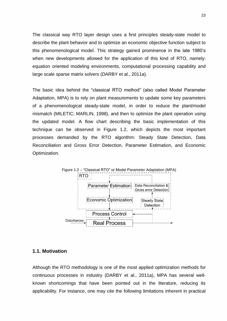
the updated model. A flow chart describing the basic implementation of this

technique can be observed in Figure 1.2, which depicts the most important

processes demanded by the RTO algorithm: Steady State Detection, Data

Reconciliation and Gross Error Detection, Parameter Estimation, and Economic

Optimization.

Figure 1.2 – “Classical RTO” or Model Parameter Adaptation (MPA)

1.1. Motivation

Although the RTO methodology is one of the most applied optimization methods for

continuous processes in industry (DARBY et al., 2011a), MPA has several well-

known shortcomings that have been pointed out in the literature, reducing its

applicability. For instance, one may cite the following limitations inherent in practical

24

implementation of model based methodologies: lack of process measurements,

measurement noise, structural plant/model mismatch, numerical optimization

(QUELHAS; DE JESUS; PINTO, 2013) and low frequency of set points update.

The first RTO drawback discussed in the present thesis is the structural plant/model

mismatch. Despite the use of high-fidelity mathematical models in the RTO layer (see

Figure 1.1), the absence of structural plant/model mismatch is not ensured. In 1985,

Biegler and coauthors discussed the use of simplified models to optimize complex

processes (which is the main idea behind the classical RTO method). They found out

that plant/model mismatch derived from the simplified model may cause problems,

since its mathematical optimum is likely to disagree with the real plant optimum.

Furthermore, they showed that an adequate model must share the same Karush-

Kuhn-Tucker (KKT) point with the real plant.

Forbes; Marlin and Macgregor (1994) introduced the concept of “model adequacy”

for the classical RTO method. They developed a procedure to determine if a model is

sufficiently flexible to represent a more complex model by a suitable choice of

adjustable parameters. In other words, the question is if there is at least one set of

parameters, for the simple model, able to yield the same economic optimum of the

complex one. Nonetheless, this adequacy criterion does not take into account the

model outputs (which should also be equal at the optimal point), causing problems in

the classical RTO algorithm, since it relies on the parameter estimation method to

reduce the plant/model mismatch (MARCHETTI, 2009). Consequently, the classical

RTO method cannot guarantee the convergence to the true process optimum under

structural plant/model mismatch.

Several methods have been developed in the literature to supposedly make the RTO

algorithm able to converge to the plant "true" optimum in spite of uncertainties.

However, they are based on plant derivatives (from process), which are quantities

difficult to obtain in the real world.

Due to uncertainties of each RTO approach, there is not a general consensus about

the reliability of different RTO methods to increase the profit of an industrial plant

(DARBY et al., 2011a). Lack of experimental and theoretical works focused on

25

evaluating the scope and limitations of different RTO approaches makes it even

harder to reach a sensible opinion about this topic. Most works available in the

literature about different RTO approaches use a few (often one) operating conditions

to draw general conclusions about the adequacy of a particular methodology.

Figure 1.3 gives an example to explain why it is necessary to consider different

process conditions to evaluate the overall performance of an RTO algorithm. In this

case, three RTO sequences (sharing the same process model) are simulated,

departing from the same starting point and trying to converge to the “optimum”

operational point, but with different uncertainty values (measurement noise and

parameters' initial guesses). For comparison, the experiments are defined as:

Blue and Red paths use the same parameter initial guesses but different measurements noise;

Black and Red paths use different parameter initial guesses but the same measurement noises.

Figure 1.3 – Illustrative example of an RTO implementation under uncertainties; (A) economic objective function value with respect to RTO iterations; (B) economic objective function profile

with respect to controlled variables (Temperature and flow rate Fb).

A B

As can be observed in Figure 1.3, the uncertainties involved in the simulations could

lead to different conclusions about the RTO performance, which requires an

approach such as Monte Carlo to draw general conclusions about the performance of

a determined method.

In the first part of the present work, the performance of the classic RTO method

(MPA) and derivative-based methods (Modifier Adaptation, MA; Integrated System

26

Optimization Parameter Estimation, ISOPE; and an algorithm based on the Sufficient

Conditions of Feasibility and Optimality, SCFO) are compared under different levels

of measurement noise, model mismatch and process disturbances, using a Monte

Carlo methodology.

The second RTO problem addressed in the present work is related to the parameter

estimation module. Theoretically, while a model becomes mathematically more

complex, and more mechanistic, it would potentially allow a broader representation

and prediction of the system behavior (which is generally expected from a RTO

model). However, the main disadvantage associated with complex models is the

amount of information (both theoretical and experimental) required to describe the

internal mechanisms, which are hindered by the noise of the available

measurements, increasing possible sources of uncertainties. In this situation,

identifiability problems are prone to take place.

Basically, the identifiability problem may result in ill-conditioning of the Hessian matrix

in the parameter estimation problem, and/or model overfitting (MCLEAN; MCAULEY,

2012), with subsequent poor predictions by the process model and, consequently,

suboptimal targets obtained by the RTO cycle. Some parameter estimation methods

are proposed in the literature to tackle the identifiability problem; however, there is

not a comprehensive review and performance comparison targeting these main

techniques. For this reason, the second part of the present work aims to provide this

review, building sufficient background to choose the most suitable parameter

estimation method for RTO implementations.

The third RTO shortcoming explored in the present work is the low frequency of set

point update. Since RTO is only performed under steady-state conditions, the plant

operates suboptimally in presence of disturbances until the detection of the next

steady-state. This is a clear disadvantage over other economic optimization

methodologies, such as Economic MPC or Dynamic Real Time Optimization, where a

dynamic model is used and it is not necessary to wait for a new steady-state before

updating the set points.

27

Considering this disadvantage, it is important for the control layer to be more tightly

coordinated with the RTO layer. In particular, the control layer must be robust

regarding common disturbances affecting the plant profit. In other words, it should

“obtain acceptable profit loss with constant set point values”. That is the definition of

Self-Optimizing Control (SOC, Skogestad, 2000), in which the main idea is to choose

a set of controlled variables that have set point values insensitive to disturbances, for

instance, state variables that are kept at active constraints despite the presence of

disturbances.

In this setting, the SOC methodology is complementary to the RTO method, and it

can be an alternative to mitigate the problem of low frequency of set point updates in

the RTO implementation (JÄSCHKE; SKOGESTAD, 2011; MANUM; SKOGESTAD,

2012). However, the practical implementation of the SOC in the MPC layer requires

the solution of some problems, such as the active set changes due to disturbances.

This limitation is also addressed in this work.

The analysis and results obtained addressing each current shortcoming of the RTO

method are combined into a prototype software for RTO implementation. Its

application is illustrated by an industrial case study of a vapor recompression

distillation process for propylene production (a particular process of the REPLAN

refinery, Petrobras). The practical implementation aspects of the RTO are detailed in

Chapter 5, considering the background information developed in previous Chapters.

1.2. Objectives

The present thesis aims to develop a more robust RTO algorithm for industrial

application. For this reason, the main weaknesses of RTO algorithms are addressed,

in order to find alternatives and overcome the most significant implementation

problems of this methodology. Each Chapter has its own objective:

1. Evaluate the performance of each RTO method to establish sensible opinion

about the advantages and disadvantages of each RTO approach;

28

2. Find the best choice for parameter estimation methodology to be implemented

in the RTO algorithm ;

3. Develop an MPC based on SOC concepts to reduce the intrinsic problem of

the low frequency of set point updates of RTO approach;

4. Discuss the practical implementation of a RTO algorithm in an industrial case

study (a vapor recompression distillation process) of the refinery REPLAN,

Petrobras.

1.3. Outline of thesis

This thesis is structured as follows: In Chapter 2, the structural plant/model mismatch

is discussed, comparing four different RTO methodologies. In Chapter 3, the

identifiability problem is addressed through comparison of four parameter estimation

techniques. Chapter 4 brings the development of a new MPC formulation with

concepts of SOC, which aims to reduce the problem of low frequency of set point

updates. Then, Chapter 5 discusses the practical implementation of the RTO

methodology in an industrial case study. Finally, general conclusions are given in

Chapter 6.

29

2. STRUCTURAL MODEL MISMATCH

One instrument used by the RTO method is the prediction of a process future

behavior through a mathematical representation, for this reason, it commonly

requires the use of high-fidelity models. However, there are many phenomenological

behaviors that are hard to be described by equation systems (e.g.: hydraulic effects

or reaction kinetics), and in these cases, simplifying hypothesis are employed in the

process modeling. Such assumptions are a source of mismatch between the process

behavior and the model prediction, resulting in inaccurate predictions and

consequently, poor performance of the RTO method.

Biegler; Grossmann and Westerberg (1985) exposed that the RTO model must have

the same Karush-Kuhn-Tucker (KKT) point than the real plant, in order to obtain the

optimum solution. Forbes and Marlin (1994) suggested that the process model must

have at least one set of model parameters resulting in the same KKT point of the real

plant to be considered "adequate". Nonetheless, the existence of this parameter set

does not guarantee that the optimum will be obtained by the closed-loop RTO. For

instance, the measured outputs could be different, as showed in a numerical

example given by Marchetti (2009). For this reason, several theoretical methods

have been developed to make the RTO algorithm able to converge to the true

optimum of the plant in spite of structural plant-model mismatch.

The first one, proposed by Roberts (1979), is a modification of the classical RTO

method called Integrated System Optimization and Parameter Estimation (ISOPE). In

this methodology the parameter estimation and the optimization steps are integrated,

resulting in a modified economic objective function for the optimization step that is

able to handle the structural mismatch problem, in cases when plant derivative can

be calculated accurately.

The second method, called Modifier Adaptation method (MA) (MARCHETTI;

CHACHUAT; BONVIN, 2009), differs from the classical RTO method in the way the

plant information is used, since the measurements are employed to fulfill the

necessary first-order optimality conditions (NOC) of the plant (using the so-called

modifiers) without updating the model parameters. The MA scheme is able to

30

calculate the plant optimum in the presence of plant-model mismatch, provided that

an accurate plant gradient is available, which, until now, is its main limitation for

industrial applications.

Bunin; François and Bovin (2013a) proposed a method to tackle the plant-model

mismatch problem, called Sufficient Conditions for Feasibility and Optimality (SCFO).

This method combines the concepts of descent half-space and quadratic upper

bound to derive sufficient conditions to guarantee the improvement of the plant

objective function at each iteration; and concepts of approximately active constraints

and Lipschitz continuity to ensure constraint feasibility at each step. Although this

method has a solid mathematical background to carry out what it claims (BUNIN;

FRANÇOIS; BONVIN, 2013b), some of its assumptions are very difficult to meet in

practice, such as the knowledge of global Lipschitz constants, global quadratic upper

bounds and the exact value of the unmeasured restrictions at the current iteration.

For this reason, Bunin; François and Bonvin (2013b) extended the SCFO method for

practical implementation. They proposed to use a feasible region for the plant

gradient to guarantee a descent region. In other words, the algorithm works within a

region where the worst case ensures a decrease in the plant objective function

without violating process constraints. However, Bunin and coworkers (2013b) state

that it is unclear if the application of SCFO is benefical, since the SCFO algorithm

may affect the convergence speed, especially when the RTO target is accurate

(provided by the MPA for instance).

Due to the limitations of each RTO approach, there is not a general consensus about

the reliability of the different RTO methods to increase the profit of a process plant

(DARBY et al., 2011b). Therefore, in the present work, a Monte Carlo methodology is

applied to evaluate the performance of each strategy under the same process

uncertainties, namely: parameter plant-model mismatch, measurement noise and

disturbances in the unmeasured variables. The Williams-Otto reactor benchmark

problem is considered as case study.

This Chapter is organized as follows: first, the particularities of four RTO methods are

presented in Section 2.1. Then, the Williams-Otto reactor case study is shown with

31

the experimental design for the Monte Carlo analysis in Section 2.2 and 2.3. The

main results are displayed in Section 2.4. and discussed in Section 2.5. Finally, the

conclusions are given in Section 2.6.

2.1. Materials and methods

2.1.1. MPA method

The structure of the classical RTO algorithm is presented in Figure 2.1. The RTO

cycle starts with the steady-state detection module, responsible to analyze the

process measurements and to decide, based on statistical criteria, if the plant has

reached steady state. Then, the stationary point goes through the data reconciliation

and gross error detection stage. Further, the screened information is used in the

parameter estimation module to update the model parameters. Then, the updated

model is employed to find a new operating point that hopefully maximizes the plant

profit. Finally, this new condition is passed to the process control layer as set points

for the controlled variables.

Figure 2.1 – Classical RTO structure

The basic statement of the optimization module can be written as:

* min

s. .

0

u

p

u = φ(u, y)

t y = F (u)

g(u, y)

(2.1)

32

where φ is the process (economic) performance index, y is the plant output, u are

the decision variables, )(uFp is the plant map, and ),( yug are the process

constrains. In the model-based RTO (MPA) the plant outputs are estimated from a

mathematical model, )F(u, , locally fitted by the estimated parameters .

ˆmin

ˆ s. . , )

ˆ 0

uu φ(u, y)

t y = F(u

g(u, y)

(2.2)

The MPA method has common vulnerabilities, namely: lack of process information

(discussed in Chapter 3), plant-model mismatch and numerical optimization issues.

(QUELHAS; DE JESUS; PINTO, 2013) However, it is the most used online

optimization method by the industry (DARBY et al., 2011b).

2.1.2. ISOPE method

One of the difficulties with the optimization problem stated in eq.(2.2) is the mismatch

between the model and the real plant. The Integrated System Optimization and

Parameter Estimation (ISOPE) method was developed to handle the structural plant-

model mismatch (BRDYS; TATJEWSKI, 2005), complementing the measurements

used in the MPA method with plant derivative information, to reduce the offset

created by the structural mismatch. ISOPE still retains the parameter estimation and

economic optimization steps as in the MPA. However, ISOPE optimizes a modified

economic function, adding a term coming from the parameter estimation step that

allows a first-order correction.

ISOPE derivation starts by reformulating the RTO problem (eq.(2.2)), and adding a

penalty term (the so-called regularization term) to the economic performance index,

u

vg

uFuF

vuuFu

p

u

0)(

)(),(s.t.

)),(,(min2

,

(2.3)

33

where ρ is the regularization parameter and v are additional variables that allow

eq.(2.3) to have essentially the same solution than the problem stated in eq.(2.1).

The Lagrange function of the optimization problem, given in eq.(2.3), is:

2 T T T

pL(u,θ,v,ξ,μ,λ)= (v,θ)+ ρ u v +ξ (F(u,θ) F (u))+ μ g(v)+ λ (u v) (2.4)

where ξ , μ and are Lagrange multipliers (or "modifiers"). The first order optimality

conditions applied to Lagrange’s function are:

0)](),([)(2 T

puu uFuFvu (2.5a)

0)()(2),( T

vv vgvuv (2.5b)

0=ξθ)(u,F+θ)φ(v, T

pθθ (2.5c)

0u v = (2.5d) 0)(),( uFuF p (2.5e)

0)( ,0 ,0)( vgvg T (2.5f)

The multipliers and , can be calculated from eq. (2.5a), (2.5c) and (2.5d)

),(),(]),(),([ 1 vuFuFuF T

(2.6)

)),(,()](),([ uFuuFuF y

T

puu (2.7)

Finally, the optimization problem solved by the ISOPE method is the modified model-

based optimization problem

0)(

),(s.t.

),(),(min2

vg

uFy

vuvuu T

v

(2.8)

where λ (u, θ) is the multiplier given in eq.(2.7). This new optimization problem has

the same optimality conditions as eq.(2.3). A comprehensive description of this

formulation is given by Brdys and Tatjewski (2005). The basic ISOPE algorithm is

shown in Figure 2.2.

34

Figure 2.2 - ISOPE structure

ISOPE has been derived assuming that the model is able to perfectly match the plant

outputs by updating model parameters (point parametric condition (ROBERTS,

1979)) and that accurate plant derivative is available. These crucial assumptions

ensure that the solution obtained by the modified model-based optimization problem

converges to the true plant optimum (MANSOUR; ELLIS, 2003). The challenges

faced by this method are the lack of process information, numerical optimization

issues, and also, the requirement of plant derivatives (the most significant problem),

which are used to compute the modifier values, since the estimation of these

quantities is considerably affected by measurement noise.(LUBANSKY et al., 2006)

2.1.3. MA method

The idea behind modifier adaptation (MA) method is to use measurements to correct

the cost and constraint predictions between successive RTO iterations in such a way

that the KKT point for the model coincides with the plant optimum (MARCHETTI,

2009).

Given the real process model (u)Fp and the RTO model F(u) , it is possible to

construct a corrected model (u)Fc similar to the real process model, eq.(2.9). The

correction term, proposed in eq.(2.10), comes from a first-order Taylor series

expansion of the discrepancy term around the current operating point, eq.(2.10). The

final corrected model is presented in eq.(2.11).

F(u)](u)[F+F(u)=(u)F pc (2.9)

35

0 0 0 0 0

p p u p uF (u) F(u)= F (u ) F(u )+ F u F u (u u )

(2.10)

)()()( 0uuuFuF T

c (2.11)

where and T are the so called modifiers, corresponds to the gap between the

plant and predicted function values, and T represents the difference between the

slopes, which are calculated as the difference between model and plant derivatives

(see eq.(2.10)). A very useful graphical interpretation of these features is presented

by Marchetti; Chachuat and Bonvin (2009).

The objective function and the constraints of the RTO problem are reformulated

using this methodology. The problem is restated as:

min

. . 0

T

c m φ k

T

c m g k

φ (u,θ)= φ (u,θ)+ λ (u u )

s t g (u,θ)= g (u,θ)+ε + λ (u u )

(2.12)

where the subscripts c and m indicate the corrected and the original RTO model,

respectively; is the economic objective function and g is the set of inequality

constraints.

Figure 2.3 - MA structure

The fundamental differences between the MA and ISOPE frameworks are how the

modifiers are calculated and the parameters updated. In MA, the modifier is

calculated from the derivatives of economic objective function with respect to inputs

(u ), while the ISOPE method uses the derivatives of outputs ( y ) with respect to the

inputs (u ). Moreover, the parameters are updated during ISOPE iterations whereas

36

MA uses a fixed parameter set during optimization, i.e., there is no parameter

updating. With this configuration, MA method also suffers from some problems as

numerical optimization issues and lack of accurate plant derivative information.

2.1.4. SCFO method

The SCFO, initially proposed by Bunin; François and Bovin (2013a) and modified for

practical implementation by Bunin; François and Bovin (2013b), adapts the nonlinear

optimization theory to RTO problems. The method is devised to calculate the plant

optimum without violating any hard constraint and improving the plant profit at each

RTO iteration, executing a projection problem based on information of plant

derivatives and topology. In other words, given a target (a possible future RTO point

predicted by any RTO algorithm, MPA for instance) the SCFO method implements a

correction to this target, based on plant derivative information. The projection

problem, given by eq.(2.13), minimizes the distance between the target ( *

1+ku ) and

the feasible point ( u ), subject to a bounded deviation ( jg,δ ) from the active

constraints ( jkj ε)(ug ) and an improvement in the objective function ( ). These

two restrictions try to maintain the solution of the projection problem ( *

1+ku ) at the

interior of the hard constraints region, given by jkj ε)(ug , and to grant a profit

improvement δ)u(u)φ(u k

T

k . This behavior is achieved within the region

where the problem nonlinearities are well approximated by the first order local

information (gradient information).

2* *

1 12

arg min

. . :

k+ k+u

T

j k k g, j j k j

T

k k

L U

u = u u

s t g (u ) (u u ) δ j g (u ) ε

φ(u ) (u u ) δ

u u u

(2.13)

where the subscript k indicates the RTO iteration, the point *

1+ku is the input target

(calculated from classical RTO approach in this work), *

1+ku is the target projected

37

into a feasible descent space, φ and jg are, respectively, the plant derivative of

the economic objective function and constraints with respect to the input variables, δ

are minimal changes required in the projected direction, and the superscripts U and

L indicate the upper and lower bound vectors.

The need for accurate real process derivatives limits the practical implementation of

this algorithm. For this reason the authors modified the projection problem to work

within a feasible region given by the derivative of the real process. These regions can

be obtained assuming a certain local structure for the economic objective function

(BUNIN; FRANÇOIS; BONVIN, 2013e), or in a less rigorous way, they may be

calculated from the estimated gradient, adding an uncertainty region around it (as

implemented in the present work). This modified projection problem is given by

eq.(2.14).

2* *1 1

, , 2

1

1

,

,

min

. .

:

:

k+ k+u S s

nu

ji g, j

i=

j

uk i k,i ji j k j

i

j

uk i k,i ji j k j

i

nu

φ,i φ

i=

uk i k,i φ i

i

uk i k,i φ i

i

u = u u

s t s δ

g| u u s j g (u ) ε

u

g| u u s j g (u ) ε

u

s δ

φ| u u s

u

φ| u u s

u

(2.14)

where s are slack variables responsible for ensuring the choice of direction for the

worst case (for objective function s and constraints S ); iu

g

and

iu

g

are the lower

and upper bounds of the constraint derivatives; iu

φ

and

iu

φ

are the lower and upper

bounds of the objective function derivatives. The main structure of the algorithm is

38

presented in figure 2.4, where the target calculation corresponds to the MPA solution

and the projection problem is performed by the solution of eq.(2.14).

Figure 2.4 - SCFO structure

2.2. Plant derivative estimation

The plant derivative is estimated from process measurements using Broyden’s

approximation formula:

))()((

)(.))(()(

11

11111 T

kkkk

kkT

kkkkkkkuuMuu

MuuuuByyBB

(2.15)

where B is the matrix of estimated derivatives, u is the vector of input variables, y

is the vector of outputs and M is a scaling (diagonal) matrix (RODGER, 2010). The

indices k and 1k indicate the current and previous steady-state points,

respectively. In this work, Broyden is preferred to methods such as finite differences

(FD) or dynamic model identification (DMI) on the basis of practical applicability,

since FD and DMI require large numbers of upsets and/or depend on the availability

of dynamic plant information, which are difficult and costly to achieve in a real

process plant (MANSOUR; ELLIS, 2003)

The Dual approach, proposed by Rodger and Chachuat (2011), is implemented in

MA and ISOPE algorithms to improve the plant derivatives estimated by Broyden’s

method, enforcing minimal perturbation in different directions (to get better

information at each step), and maximum step length (to avoid the “peak

phenomenon”, as discussed by Rodger (2010)). This approach is implemented by a

39

set of constraints (eq.(2.16) and (2.17)), which determine two possible regions for

solution search.

1

01

k

T

k

k

T

kkk

uuuu

wwuuw (2.16)

1

01

k

T

k

k

T

kkk

uuuu

wwuuw (2.17)

where ku and u are the current and future RTO points, respectively, kw is an

unitary vector orthogonal to the last two RTO points, is the parameter matrix for

the minimum upset and is the parameter matrix of maximum step length. In this

work the values of B and are 4.050diag and 15.040diag respectively.

In the Dual approach, the economic optimization problem is divided in two problems,

one defined by eq.(2.16) and other by eq.(2.17). Then, these problems are

simultaneously solved and the best result is implemented. A graphical interpretation

can be found in Rodger and Chachuat (2011).

2.3. Case study: Williams Otto reactor

The Williams Otto CSTR (continuous-stirred tank reactor) is a well-known case study

that has been used for the development and comparison of RTO strategies by

several authors (MARCHETTI; CHACHUAT and BONVIN, 2009; PFAFF, 2001;

ZHANG; NADLER and FORBES, 2001). This process is illustrated in Figure 2.5. The

reactor is fed with Fa and Fb (pure streams of components A and B, respectively),

these components react producing an intermediate component C, which reacts with

another B molecule to produce the desired products P and E. There is a side reaction

between components C and P, producing a waste byproduct G that has zero

commercial value. The reactions and their kinetics are given in eq.(2.18).

40

Figure 2.5. - Williams Otto reactor

1 1 exp( 1 / ( 273.15))

2 2 exp( 2 / ( 273.15))

3 3 exp( 3 / ( 273.15))

R

R

R

A B C k p Ea T

B C P E k p Ea T

P C G k p Ea T

(2.18)

where Ea , the activation energy and ηp , the pre-exponential factor, are given in

Table 2.1.

The process is modeled at steady-state by the mass balances, using the reactor

temperature (TR) and flow rate of B (Fb) as controlled variables, and keeping the flow

rate of reactant A (Fa) and the mass holdup (W) at 1.8275 kg/s and 2105 kg,

respectively. The economic objective is to maximize the profit USD/s given by

eq.(2.19).

BARERP FFFXFX 34.11423.7692.2538.1143 (2.19)

where XP and XE are the mass fractions of P and E, respectively, in the reactor outlet

stream (FR).

To analyze the performance of each RTO methodology under structural plant-model

mismatch, a simpler kinetic (approximated model) is proposed to describe the original

system (FORBES; MARLIN and MACGREGOR, 1994) (eq.(2.20)).

))15.273/(2exp(22

))15.273/(1exp(112

R

R

TkGCP

TkEPBA

(2.20)

41

where ν is the activation energy and η is the pre-exponential factor, both estimated

by the parameter estimation module.

2.3.1.1. Parameter estimation module

In our analysis we consider a perfect and an approximate model, eq.(2.18) and (2.20)

respectively. In both cases, all kinetic parameters (pre-exponential factors and

activation energies) are estimated using the product compositions Xp, Xe and the flow

rate, Fa, as measurements. This is due to the fact that it is very unlikely that a real

plant has online measurements of all products compositions (online composition

measurements are very expensive). The objective function corresponds to an

unweighted least squares problem. Furthermore, the last three historical points in the

RTO path are used by the parameter estimation module, as suggested and

implemented by Pfaff (2001), to increase the amount of information.

2.3.1.2. Experimental Design

The present section aims to design a comprehensive experiment to evaluate the

algorithms performance over a wide range of different situations. For this reason, we

consider five process characteristics that can modify the evaluation of a RTO

algorithm. The first two problems are related to the parameter estimation module:

measurement noise and the initial values of parameters. Both may deteriorate the

parameter estimation and change the RTO path, resulting in different performances

for the same RTO algorithm. The influence of these random variables is assessed

through Monte Carlo simulations, where 500 RTO trials are carried out using different

initial values of the parameters and measurement noise sampled following uniform

and normal distributions, respectively (see Appendix A).

The third and fourth problems are disturbances presented in measured and

unmeasured variables. These process characteristics are simulated in the plant by

changing the parameter listed in Table 2.1, which results in four regions depicted in

Figure 2.6 The first and second disturbance steps correspond to changes in the

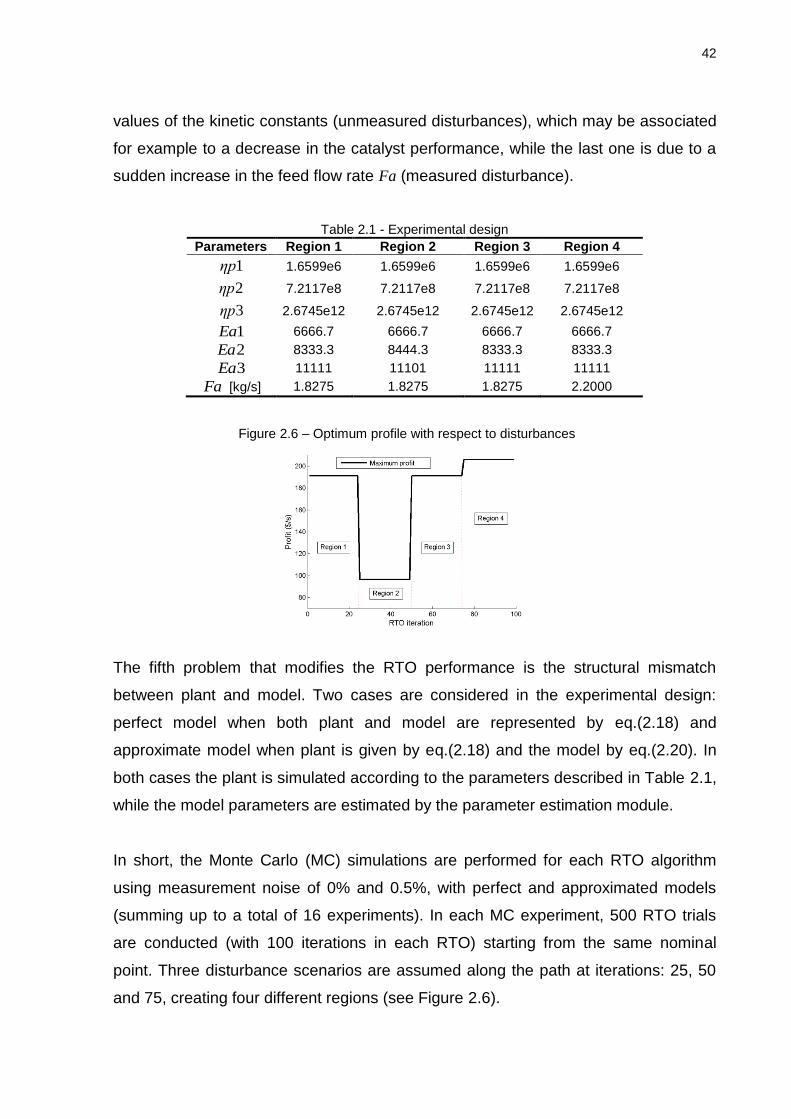
42

values of the kinetic constants (unmeasured disturbances), which may be associated

for example to a decrease in the catalyst performance, while the last one is due to a

sudden increase in the feed flow rate Fa (measured disturbance).

Table 2.1 - Experimental design

Parameters Region 1 Region 2 Region 3 Region 4

1ηp 1.6599e6 1.6599e6 1.6599e6 1.6599e6

2ηp 7.2117e8 7.2117e8 7.2117e8 7.2117e8

3ηp 2.6745e12 2.6745e12 2.6745e12 2.6745e12

1Ea 6666.7 6666.7 6666.7 6666.7

2Ea 8333.3 8444.3 8333.3 8333.3

3Ea 11111 11101 11111 11111

Fa [kg/s] 1.8275 1.8275 1.8275 2.2000

Figure 2.6 – Optimum profile with respect to disturbances

The fifth problem that modifies the RTO performance is the structural mismatch

between plant and model. Two cases are considered in the experimental design:

perfect model when both plant and model are represented by eq.(2.18) and

approximate model when plant is given by eq.(2.18) and the model by eq.(2.20). In

both cases the plant is simulated according to the parameters described in Table 2.1,

while the model parameters are estimated by the parameter estimation module.

In short, the Monte Carlo (MC) simulations are performed for each RTO algorithm

using measurement noise of 0% and 0.5%, with perfect and approximated models

(summing up to a total of 16 experiments). In each MC experiment, 500 RTO trials

are conducted (with 100 iterations in each RTO) starting from the same nominal

point. Three disturbance scenarios are assumed along the path at iterations: 25, 50

and 75, creating four different regions (see Figure 2.6).

43

The performance of the RTO methodologies are compared using three statistics

computed from the profit error, namely: root mean square error, average profit loss

(absolute value) and frequency to obtain profit loss less than 1% in the last 5 RTO

iterations of each region (%). In this work the profit loss is defined as the difference

between the instantaneous profit using the set points calculated by the RTO and the

true optimum in each region defined in Figure 2.6.

Appendix B shows the performance of each RTO method under perfect conditions.

These experiments are important to illustrate that the algorithms work well under

ideal conditions and their implementation was done correctly.

2.4. Results

2.4.1. Results for perfect model

Figure 2.7 presents the results of the four RTO methods using noise-free

measurements and perfect model. In this figure the frequency distribution of the

economic objective function is denoted by the color scale.

The behavior shown in Figure 2.7 and the dispersion metric presented in Table 2.2

indicate that the MPA method presents the lowest scattering profile, since this

method is not influenced by the errors in the derivative caused by the Broyden’s

approximation that affects all the derivative-based methods tested. Among these

strategies, the SCFO exhibits the lowest dispersion.

The frequency of attaining the optimum profit (within 1 %) in the last 5 RTO iterations

is shown in Table 2.3. It can be appreciated that the MPA methodology follows the

optimum plant operation path along the different plant upsets. In this case, the

information quality as well as the model structure allow the parameter estimation

routine to identify a topology converging to the “true” optimum in few RTO cycles

(around 15 cycles on average), even after plant disturbances.

44

Regarding the profit loss during the RTO, the path followed by MPA is the most cost

effective (on average 3.04 USD/s), since it presents lower profit loss than any

derivative based method tested. SCFO shows the best result for the first region (see

Table 2.4), basically because it has the largest first step among the methods;

however its average profit loss is 4.64 USD/s.

Figure 2.7 – MC experiments using noise free measurements and perfect model: (A) MPA, (B) MA,

(C) ISOPE and (D) SCFO

A

B

C

D

Table 2.2. - Root mean square error for MC experiments using noise free measurements and perfect model

Method Region 1 Region 2 Region 3 Region 4

MPA 8.15 4.59 8.36 9.13 MA 8.44 7.35 10.61 11.58

ISOPE 8.15 6.31 10.89 12.24 SCFO 8.68 5.07 8.81 9.83

45

Table 2.3. - Frequency of achieving less than 1% profit loss in the last 5 RTO iterations of each region. MC experiments using noise free measurements and

perfect model.


MPA 100 100 100 100 MA 72.16 43.36 60.48 84.80

ISOPE 55.00 39.24 56.16 79.24 SCFO 86.48 28.72 76.84 67.08

Table 2.4. - Average profit loss for MC experiments using noise free measurements and perfect model

Method Region 1 [USD/s]

Region 2 [USD/s]

Region 3 [USD/s]

Region 4 [USD/s]

MPA 8.50 0.78 1.33 1.56 MA 8.90 5.44 6.30 5.57

ISOPE 9.33 4.23 6.88 7.88 SCFO 7.59 3.78 3.06 4.13

The results for the MC simulations with perfect model and measurement noise are

shown in Figure 2.8. A comparison of the statistics of the RTO performance using

noisy measurements (Tables 2.5 to 2.7) with previous noise free measurements

(Tables 2.2, 2.3 and 2.4) indicates a lower performance of the RTO methodologies

due to corrupted information.

The comparison of the RTO methods with and without measurement noise shows

that , as expected, noise always increases profit loss (cf. Tables 2.4 and 2.7). As in

the noise-free case, the MPA is the one with the lowest profit loss on average, this

loss is even lower than the ones achieved by the derivative based methods using

perfect measurements.

Table 2.5. - Root mean square error for MC experiments using noisy measurements (0.5%) and perfect model


MPA 9.95 5.19 8.59 9.34 MA 9.40 8.61 10.81 12.54

ISOPE 8.95 9.11 11.14 13.33 SCFO 9.97 5.09 6.36 9.91

Table 2.6. - Frequency of achieving less than 1% of profit loss in the last 5 RTO iterations of each region. MC experiments using noisy measurements (0.5%) and

perfect model


MPA 75.44 44.96 79.08 80.84 MA 28.08 11.20 23.36 32.12

ISOPE 25.72 12.20 22.08 28.56 SCFO 25.32 18.60 28.96 17.96

46

Table 2.7. - Average profit loss for MC experiments using noisy measurements (0.5%) and perfect model


Region 2 [USD/s]

Region 3 [USD/s]

Region 4 [USD/s]

MPA 9.72 2.96 1.98 2.87 MA 11.72 8.42 8.14 10.14

ISOPE 11.60 8.08 8.63 11.41 SCFO 9.97 5.09 6.36 9.91

Figure 2.8 – MC experiments using noisy measurements (0.5%) and perfect model: (A) MPA (B) MA (C) ISOPE and (D) SCFO

A

B

C

D

2.4.2. Results for the approximated model

These experiments assess the behavior of the RTO methodologies under structural

plant-model mismatch. The results obtained in the Monte Carlo simulations using the

approximate model and noise free measurements are depicted in Figure 2.9. The

structural mismatch does not allow the convergence of the MPA method to the true

47

optimum in all regions, which is confirmed by low frequency of obtaining profit losses

less than 1% (see Table 2.9). In contrast, the derivative based methods are able to

handle the structural mismatch in all tested regions, as can be observed in Figure 2.9

and Table 2.9.

The scattering presented by MPA and SCFO tend to be alike in every region, this

dispersion is lower than the obtained by the MA and ISOPE under similar conditions

(see Table 2.8). However, the lower average profit loss corresponds to the path

followed by MA in the first region, MPA in the second region and by SCFO in the third

and fourth regions (see Table 2.10). On average SCFO presents the best economic

results.

Figure 2.9 – MC experiments using noise free measurements and approximate model: (A) MPA (B) MA (C) ISOPE and (D) SCFO

A

B

C

D

48

Table 2.8. - Root mean square error for MC experiments using noise free measurements and approximate model


MPA 8.00 4.58 8.22 9.22 MA 8.32 7.61 10.74 11.47

ISOPE 8.09 5.90 11.25 12.22 SCFO 8.45 5.51 8.99 9.66

Table 2.9. - Frequency of achieving less than 1% profit loss in the last 5 RTO

iterations of each region. MC experiments using noise free measurements and approximate model


MPA 1.12 0.00 0.00 0.00 MA 73.40 42.28 62.72 81.44

ISOPE 57.80 37.76 54.28 74.56 SCFO 73.52 13.04 64.28 65.24

Table 2.10. - Average profit loss for MC experiments using noise free measurements and approximate model


Region 2 [USD/s]

Region 3 [USD/s]

Region 4 [USD/s]

MPA 10.90 3.15 7.64 5.97 MA 8.92 5.61 6.44 5.31

ISOPE 9.84 3.77 7.55 7.72 SCFO 9.28 5.77 3.74 3.94

Figure 2.10 shows the outcome of the MC simulations for the case using the

approximate model and measurement noise of 0.5%. The results point out

increasing scattering of the RTO path compared to the case with same structural

model mismatch and noise-free measurements (Tables 2.8 and 2.11). Another fact

observed is that the derivative-based methods are more sensitive to noise than the

MPA method. Indeed, the profit loss increases around 45% for MA and 36% for

ISOPE and SCFO methods, in comparison with an approximate decrease of 18%

presented by MPA under the same conditions (Tables 2.10 and 2.13).

The MPA, as observed in the MC simulations using an approximate model and noise

free measurements, presents offset between the predicted optimum and the real one

in the first three regions, this behavior reduces the frequency of obtaining profit

losses less than 1% in these regions using MPA rather than the derivative-based

methods (Table 2.12). However, this method outperforms the derivative-based

approaches in region 4 where the offset is not present.

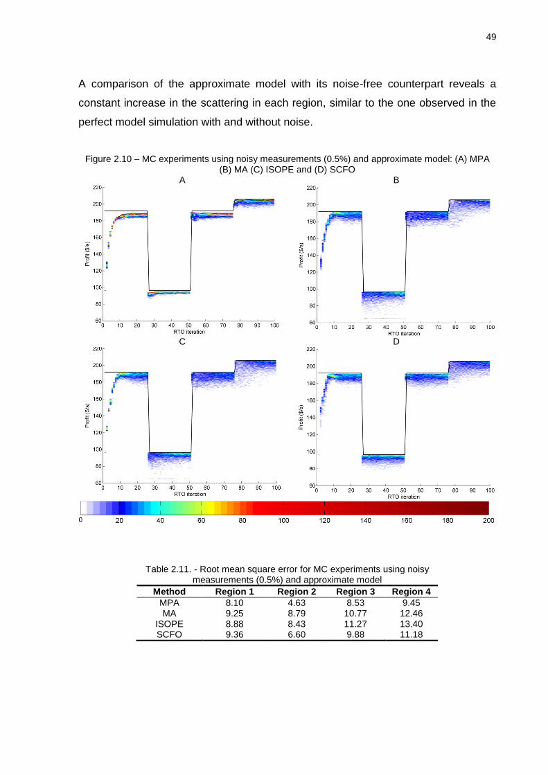
49

A comparison of the approximate model with its noise-free counterpart reveals a

constant increase in the scattering in each region, similar to the one observed in the

perfect model simulation with and without noise.

Figure 2.10 – MC experiments using noisy measurements (0.5%) and approximate model: (A) MPA (B) MA (C) ISOPE and (D) SCFO

A

B

C

D

Table 2.11. - Root mean square error for MC experiments using noisy measurements (0.5%) and approximate model


MPA 8.10 4.63 8.53 9.45 MA 9.25 8.79 10.77 12.46

ISOPE 8.88 8.43 11.27 13.40 SCFO 9.36 6.60 9.88 11.18

50

Table 2.12. - Frequency of achieving less than 1% profit loss in the last 5 RTO iterations of each region. MC experiments using noisy measurements (0.5%) and

approximate model


MPA 1.44 0.00 1.92 49.44 MA 27.48 13.72 23.60 31.28

ISOPE 27.32 11.84 20.44 28.96 SCFO 25.20 15.96 26.56 25.16

Table 2.13. - Average profit loss for MC experiments using noisy measurements (0.5%) and approximate model


Region 2 [USD/s]

Region 3 [USD/s]

Region 4 [USD/s]

MPA 11.47 2.67 4.84 3.75 MA 11.66 8.11 8.15 10.25

ISOPE 11.98 7.49 8.74 11.10 SCFO 9.88 5.51 6.64 8.95

2.5. Discussion

The Monte Carlo simulations using a structural perfect model points out that MPA

performs better than derivative-based methods in the presence of disturbances and

measurement noise. This result is partially due to the fact that the experimental

conditions fulfill the assumptions made for the parameter estimation method, since

the least squares estimator is able to handle noisy data composed of independent,

normally distributed zero-mean measurements (PFAFF, 2001). On the other hand, it

would be expected a poor performance of the Least Squares estimator, and in the

overall performance of the MPA method, in cases where measurements are

corrupted with gross errors or correlated noise. In these cases, redescending or

appropriate likelihood estimators should be used (ARORA; BIEGLER, 2001).

The approximate model used in the second analysis fulfills the adequacy criterion of

Forbes; Marlin and Macgregor (1994), since there is at least one set of parameters

that predicts the same optimal point than the plant (at least for regions 1 and 3).

However, Marchetti (2009) pointed out that for this set of parameters the model

outputs differ from the plant output, becoming unlikely to converge to the “ideal” set

of parameters through a parameter estimation and optimization approach (MPA

method).

51

The results obtained in the MC simulations using the approximate model and noise

free measurements suggest that MPA is unable to converge to the true optimum, in

consequence, the derivative-based RTO methods (SCFO and MA) have better

economic performance. On the other hand, MPA shows better economic

performance than derivative-based methods in cases where optimization runs under

measurement noise and plant-model mismatch. Also in this case, in the fourth region,

MPA does not present offset, since the model is able to simulate the process

topology.

The improvement observed in the MPA method is related to the parameter estimation

module, since the upsets introduced by the measurement noise are sufficient to

increase the sample distribution quality, obtaining better information. Similar results

could be achieved by introducing the Dual methodology to the MPA approach. Figure

2.11 shows a comparison between MPA with and without the Dual methodology. One

can note that Dual approach decreases the bias observed in the RTO path calculated

by the MPA method, consequently decreasing the profit loss by approximately 28%

with respect to MPA without Dual approach.

Figure 2.11. - Comparison between MPA with approximate model and free measurement noise. (A) MPA without Dual approach; (B) MPA with Dual approach. (A)

(B)

The derivative-based methods present better results than the MPA only in the case

of model mismatch and noise free measurements. In particular, the SCFO method

presents the best economic performance among the derivative-based methods,

followed by the MA and then ISOPE. This fact indicates that SCFO is better designed

to handle the uncertainty introduced by the Broyden’s estimation. In comparison with

52

ISOPE, MA shows a slightly better performance, indicating that the parameter

estimation module is not necessary for this approach type.

In general, the results show that derivative-based methods are more sensitive to

measurement noise than the classical MPA method. In fact, the conditions used in

the numerical experiments are especially difficult for the derivative-based methods,

since the random sampling of parameters (in the first iteration - Appendix A) is likely

to produce significant plant-model mismatch from the first RTO iteration, therefore the

approximation given by Broyden is prone to produce a misleading search direction

from the beginning of the RTO iterations. Another factor affecting Broyden’s methods

performance are the “drastic” changes in process topology induced by the sudden

disturbances added in the experiments during the RTO iterations. For instance, see

that the dispersions obtained by MA and ISOPE in regions 1 and 3 are notoriously

different even though the plant parameters are the same in both regions (Figure. 2.7

and 2.9). In the first region, the algorithm starts from a unique point where the

derivatives are estimated by the model, at a corner point where the derivative module

is large and points approximately to the optimum solution while region 3 may start at

several different points (end points of second region). In comparison to this region 1,

the starting points of region 3 are placed in a flatter area, which decrease the quality

of Broyden's derivative prediction.

The influence of measurement noise on the gradient prediction is analyzed through a

simple experiment and consists in calculating a sequence of gradient approximations

using Broyden’s method, under different levels of noise. The quality of the gradient

estimate is evaluated using the angle and the norm ratio between the predicted and

the true gradient. Figure 2.12 shows the influence of the measurement noise over

these two characteristics, for a sequence of four RTO iterations, starting from the

same point and converging to the optimum (#1 blue, #2 green, #3 red and #4 black),

using noises of 0 (Figure 2.12 A and B), 0.05% (Figure 1.12 C and D), 0.5% (Figure

1.12 E and F) and 1% (Figure 1.12 G and H).

53

Figure 2.12. - Derivative analysis: (A – C – E - G) angle distribution between true and predicted gradient; (B – D – F - H) Norm ratio distribution between true and predicted gradient

A

B

C

D

E

F

G

H

For the noise free case, the maximum average angle between the predicted plant

gradient using Broyden and the true is less than 2 degrees, meaning that Broyden

approximation is close to the true local direction of maximum function increase.

Moreover, for this case the predicted derivative norms are similar to the true one,

54

indicated by a norm ratio close to 1 in Figure 2.12 B. Under these conditions, viz.

noise free and good initial guess, Broyden’s approximation shows a reasonable

estimation of the plant gradient.

The increment in the angle between the true and the estimated gradient confirms the

high sensitivity of Broyden’s method to measurement noise (Figure 1.12 A, C, E and

G). Also the increase of the scattering at each RTO step indicates high sensitivity to

information degradation (i.e. measurement noise); this behavior can be better

appreciated in cases with 0.5% and 1% of noise, where the norm ratios between the

derivatives are highly scattered, affecting the step length taken toward the optimum

by the derivative-based RTO routine.

The high sensitivity to measurement noise of Broyden’s gradient estimation (even for

measurement noises as low as 0.5%) is a serious pitfall for its implementation in

practical situations, and is the reason why several alternative approaches have been

devised to improve the plant gradient estimation (BUNIN; FRANÇOIS and BONVIN,

2013c; MANSOUR; ELLIS, 2003). An interesting alternative is to take advantage of

the transient periods to get more information from the plant (GRACIANO; MENDOZA

and LE ROUX, 2014). Some techniques are known to use this information as

identification of linear or nonlinear dynamic models used to predict plant gradients

(BAMBERGER and ISERMANN, 1978), which can be implemented without affecting

the basic (derivative-based) steady-state RTO scheme, probably improving the

performance of this method.

2.6. Partial Conclusions

The main findings of this chapter can be summarized as:

i) The MPA presents the best performance among the methods compared, for the

perfect model case. This method shows the lowest profit loss in the studied

scenarios. The key point in this method, provided a flexible enough model to

generate the local process topology, lies on using a parameter estimation method

capable to minimize the overfitting caused by the lack of practical identifiability

55

(BARD, 1974). On the other hand, for the approximate model experiments, MPA

presents better results than the derivative-based method in cases with measurement

noise or when a specific method (e.g., Dual methodology) is used to improve the

sample information quality.

ii) The plant derivative predicted by Broyden’s method is highly sensitive to

measurement noise and to initial estimates of the derivatives. The SCFO is the most

suitable method to handle this kind of uncertainty, presenting the best economic

results. The comparison between MA and ISOPE shows that the parameter

estimation module is less important than the derivative quality, for this kind of

approach.

In conclusion, the results show that classical RTO method can be reasonably reliable

provided a model flexible enough to mimic process topology, a parameter estimation

method suitable to handle process noise characteristics (better discussed in next

chapter), gross errors and lack of model identifiability and a method to generate

process upsets to improve the sample information quality (Dual methodology).

The implementation of a derivative-based RTO method, in cases of evident model

mismatch, should be considered only if the gap between the predicted and the real

optimum is large enough (which is impossible to know a priori) and the level of

measurement noise is low. Furthermore, other aspect to be considered is the need

for implementing better techniques to estimate the plant gradient using transient

information.

Considering these outcomes, only the MPA method is considered for implementation

in the industrial case study, which is carried out in Chapter 5 of the present thesis.

The paper “Assessing the Reliability of Different Real-Time Optimization

Methodologies”, which was accepted for publication in Canadian Journal of Chemical

Engineering, presents the main findings shown in Chapter 2.

56

3. PARAMETER ESTIMATION

The success of an RTO implementation is directly correlated with the accuracy of the

mathematical model used to represent the plant behavior; therefore detailed models

are commonly employed in this approach.

Mathematical models can be classified with regard to the relative amount of

knowledge of the internal mechanisms used to describe a specific process, ranging

from empirical (black box), to semi-empirical (grey box) and mechanistic (white box)

models (HANGOS and CAMERON, 2001). Empirical models are entirely based on

experimental input/output information without taking into consideration any

information about the internal mechanisms of the system, while mechanistic models

are derived from the knowledge of the basic principles governing a specific process.

Semi-empirical models are in between, since they include both basic principles and

experimental information (used to fit purely mathematical correlations). The degree of

complexity of a model increases as it includes more basic principles, i.e., as it

incorporates more mechanistic description.

Theoretically, while a model becomes mathematically more complex and more

mechanistic, it would potentially allow a broader representation and prediction of the

system behavior, becoming more interesting from the point of view of RTO. However,

the main disadvantage associated with complex models is the amount of information

(both theoretical and experimental) on the internal mechanism. Available

measurements noise hinders the reliability of such information, which widens the

possible sources of uncertainties and may result in identifiability problems.

A model is said locally (globally) identifiable when the objective function of the

parameter estimation problem, e.g. least squares, has a local (global) minimum at an

isolated point (NGUYEN and WOOD, 1982). The model identifiability can be

analyzed from structural and practical points of view. The first one assesses if the

functional form of the model (model structure) permits the determination of a unique

parameter set from noise-free measurements whereas the second evaluates if the

quality (e.g., measurement noise) and quantity (statistical degrees of freedom e.g.,

57

few measured states in a bio/chemical reactor) of the available measurements allow

such a determination in practice (BELLMAN; ÅSTRÖM, 1970; RAUE et al., 2009).

The lack of structural identifiability implies lack of practical identifiability, but the

converse is not true (MIAO et al., 2011), since structurally identifiable models might

not be identifiable in practice due to the limitations imposed by the quality and

quantity of the available measurements and by the numerical difficulty to find the

local minimum.

Even if a model is structurally identifiable, model predictions can be extremely

insensitive to some individual parameters and their combination. One of the main

consequences of this is the ill-conditioning of the Hessian matrix in the optimization

problem used to find the estimate. The ill-conditioning can make the solution of the

optimization problem impossible to obtain (MCLEAN; MCAULEY, 2012).

However, even if the solution could be calculated accurately (in a numerical sense,

i.e., if the computational precision could be increased adequately in order to obtain

precise results in spite of severe ill-conditioning) the solution is contaminated by

overfitting. As a consequence, the regression coefficient vector estimated by the

least squares is expected to be far from the real parameter vector, and negligible

changes in data can cause the least squares solution coefficients to assume very

large absolute values and even to reverse signs (MARQUARDT, 1970).

In order to tackle the practical identifiability problem, two approaches can be

conceived, simply stated as follows: obtaining more experimental information by

generating more data points spanning different operating conditions or modifying the

model estimation procedure, and applying mathematical strategies without neither

adding new experimental data nor modifying the experimental procedure. The first

approach tends to be costly, time consuming and sometimes physically infeasible,

therefore a great deal of effort has been devoted to find methods to tackle the

practical identifiability problem using the least amount of experimental data.

An approach to successfully reduce uncertainty in parameters can be obtained by

providing a priori information about the physical process, model parameters or the

58

estimator. This information can be used to modify the model structure (e.g. model

reduction, reparameterization) or to identify a subset of identifiable parameters (for

instance, via sensitivity analysis) (MIAO et al., 2011).

Model reduction methods aim to reduce the model complexity using simplifying

assumptions to decrease the number of equations, and consequently, the number of

parameters that should be estimated (KEESMAN; SPANJERS; STRATEN, 1998;

NIKEREL et al., 2009; TJÄRNSTRÖM; LJUNG, 2002). It can be shown that this

approach can be equivalent to introducing false a priori information, but it is a

common practice (LE ROUX, 1995). A consequence of using model simplifications is

that the reduced model might not represent a wide range of conditions as the original

one would.

In the reparameterization approach, the original model is rearranged grouping some

parameters in order to reduce its number. It is said that this approach, as well as the

model reduction, requires expertise to obtain a suitable transformation (BIEGLER;

DAMIANO; BLAU, 1986; SURISETTY et al., 2010). However, this problem has major

analogies with the problem of finding what vectors to select as a basis in a rank

deficient linear algebra problem.

Benzvi (2008) proposed a reparameterization method for unidentifiable models via

differential geometry, in which the reparameterization is implemented by developing

a transformation that divides the parameter space into an estimable and an

inestimable part. The estimable part of the parameter space is chosen based on a

priori information about the system. This method does not require sensitivity

calculations and is applicable over a wide variety of experimental conditions.

Sensitivity-based methods tackle the identifiability problem by determining the

influence of the model parameters in the model outputs. In this way, it is possible to

select which parameters should be fitted from the available information. These

sensitivities can be classified as global and local; the former serve to quantify the

parameter influence over the whole search space, whereas local sensitivities show

parametric influence locally (CHU; HUANG; HAHN, 2011; HAAKER; VERHEIJEN,

2004). The main drawback using local sensitivities is that they may change from

59

point to point in the search space, therefore there is no certitude about the real

importance of a parameter in the model. This issue becomes critical when

sensitivities are the only criterion to decide which parameter subset should be

adjusted by the available information. On the other hand, global sensitivities provide

an unambiguous picture of the importance of a parameter in the model, at the

expense of a higher computational cost, thus, global sensitivities are employed to

study the general behavior of mathematical models rather than to determine a

specific solution (SOBOL, 2001), which is not relevant in the present work.

Miao and coworkers (2011) reported four typical local-sensitivity-based methods:

correlation method, principal component analysis (PCA) method, eigenvalue method

and orthogonal method. They point out that the last two methods outperform the first

two, because they are better designed to evaluate and compare the influence of the

parameter values in the system outputs (QUAISER; MÖNNIGMANN, 2009).

A simple and useful eigenvalue-based method is the rotational discrimination

algorithm (FARISS; LAW, 1979). This method performs a decomposition of the

search space, such that it projects the least-squares direction onto a reduced space,

where the objective function decreases the most. The issue of near-singular Hessian

matrix, typical of unidentifiable systems, is addressed by spectral decomposition.

Thus, the search direction restricted to a principal-component projection helps to

reduce model overfitting, compared to an unbiased parameter estimator.

The combination between orthogonality and eigenvalue analyses gives rise to a

family of methods that automatically adjust a subset of model parameters, while

keeping the others at arbitrary nominal values. The challenge in this approach is to

choose a parameter subset to fit the model, since the available data must be used to

adjust the most relevant parameters. The objective of these methods is to determine

how many and which parameters should be chosen to compose the subset of

adjustable parameters.

Estimation methods based on automatic selection of parameters have been an

intensive research field. Initially, Weijers and Vanrolleghem (1997) suggested a

method to evaluate all possible permutations of model parameters, using the

60

determinant and condition number of the Fisher Information Matrix (FIM) to choose

the best parameter subset to fit the model. Li and coworkers (2004) presented a

parameter ranking methodology based on eigenvalue and orthogonality criteria.This

algorithm starts with a PCA of FIM to find the most sensitive parameters, then, it

continues choosing the parameters with lower linearity index in relation to the

parameters already chosen (using an orthogonality analysis), until completing the

parameter subset to adjust the model. The number of elements in this subset was

heuristically selected. Later, Lund and Foss (2008) proposed a method to determine

the ideal number of elements in the parameter subset employing variance

contribution analysis. Secchi and coworkers (2006), on the other hand, improved the

algorithm created by Li et al. (2004) employing predictability degradation and

parameter correlation indexes, that gave rise to an algorithm for automatic selection

of the parameter subset used to adjust the model.

In this work, the performance of four methods representing different parameter

estimation approaches (Rotational discrimination, RD (FARISS; LAW, 1979),

Automatic parameter selection, APS (SECCHI et al., 2006), reparameterization via

differential geometry, RDG (BEN-ZVI, 2008) and the classic nonlinear least squares,

LSq) are assessed in terms of quality of the parameters obtained (understood as the

prediction capacity of the model on a validation set), robustness and speed, using a

Monte Carlo (MC) strategy. The outcome of this study is useful to evaluate the

suitability of these methods to handle unidentifiable models, commonly encountered

in real time optimization problems and in online state identification, where parameters

are constantly updated from limited and noisy measurements.

The present Chapter is ordered as follows: the selected estimation methods are

described in Section 3.1, Section 3.2 discusses the local parametric sensitivity

method, Section 3.3 and 3.4 are devoted to explain the case studies. The main

findings are presented and discussed in Sections 3.5 and 3.6, respectively. Final

considerations and conclusions drawn from this study are given in Section 3.7.

61

3.1. Practical identifiability improvement approaches

This section is aimed to present fundamental aspects of the methods employed in

this work to improve practical identifiability. An in depth treatment of each method

can be found in the original works.

3.1.1. Reparameterization via differential geometry (RDG)

Ben-zvi's method (BEN-ZVI, 2008) is used for reparameterizing non-linear systems

by identifying a priori process quantities that have strong impact on model

predictions. These process quantities will be accurately estimated even if specific

model parameters are not.

The pseudo-outputs are used to partition the parameter space , into estimable ,

and inestimable , subspaces. The parameters belonging to the estimable

subspace are likely to be estimated from available measurements, while parameters

in the inestimable subspace are not. Optimizing in the coordinates has the

following properties (BEN-ZVI, 2008): i) the parameters are estimable, ii) the

parameters are inestimable and iii) parameters and are independent. This

condition is given by the orthogonality criterion 0,

ij dd , where . denotes the

scalar product between the derivatives of the jth pseudo output of the estimable (

jd )

and the ith pseudo output of the inestimable subspaces (

id ). Pseudo output

derivatives are calculated from the partial derivatives with respect to the parameters

, i.e.

j

jd and

iid .

The nonlinear transformation employed by Ben-zvi to reparameterize the original

model is insensitive to the choice of experimental conditions and parameter

estimates. Furthermore, it does not require the cause or mechanisms of inestimability

to be identified. The main features of the method are summarized in the following

algorithm (see Figure 3.1).

62

Figure 3.1 - Main steps of the RDG method.

Ben-zvi's Algorithm

1. Given a model with a parameter set .

2. Identify pseudo-outputs ( ): Pseudo-outputs are process quantities (non-linear

combinations of parameters and/or states) that have strong impact on model

predictions. Pseudo-outputs will be, in the general case, functions of both

parameters and state variables; in this case pseudo-outputs should be evaluated

using nominal values of the states.

3. Use pseudo-outputs and coordinate transformation to partition the parameter

space into an estimable, , and inestimable, , subspace so that the space

T , is a local diffeomorphism and 0,

ij dd . This condition implies

that optimizing over all parameters is approximately equivalent to optimizing over

while holding at fixed values.

4. Optimize over while holding at fixed values. The optimization problem in the

coordinates is well posed, computationally efficient, and the estimates obtained

for are independent of the fixed nominal values used for .

5. Obtain the original parameter set from the mapping .

63

It is worth noting that there is not a unique way to select the pseudo-outputs because

it is an election done by the user, based on a priori knowledge of the specific case.

Further details are provided in Appendix C.

3.1.2. Rotational discrimination (RD) method

This method uses the spectral decomposition of the search space to deal with the

near singularity of the Hessian matrix. It projects the least-squares direction onto a

reduced space where the objective function decreases the most.

Given the optimization problem of the parameter estimation as:

1

1

min ( ) ( ) ( )

. . :

m

j j j

j

f r v r

s t l u

(3.1)

where ℝn is the vector of parameters, 1 2( ) [ ( ), ( ),..., ( )]T

mr r r r is the residual

vector. In this specific case, it is the difference between the model prediction and the

measured value, 1,2,...,ˆ( ) ( ( ) )j j j j mr y y .

jv is the diagonal matrix of measurement

variance, l and u are the parameter lower and upper bounds, respectively.

The derivatives of ( )f , ( )f and 2 ( )f , can be written as function sensitivities

of r ,1,2,...,

1,2,...,

( )j

j mi

i n

rS

, as stated by eq.(3.2) and (3.3).

1 1

1

( ) ( ) 2 ( ) ( ) 2 ( ) ( ) ( )m

T

j j j

j

f g r v r S V r

ℝn (3.2)

2 1 1 2

1 1

1 1 2

1

( ) ( ) 2 ( ) ( ) 2 ( ) ( )

2 ( ) ( ) 2 ( ) ( )

m mT

j j j j j j

j j

mT

j j j

j

f H r v r r v r

S V S r v r

ℝ

n X n (3.3)

64

Since the first term of the last equation is often dominant, the second may be

neglected, either because of near-linearity of the model close to the solution or

because of the residuals are small (NOCEDAL; WRIGHT, 1999). As a result, the

second derivative of ( )f is simply given by:

2 1( ) ( ) 2 ( ) ( )Tf H S V S ℝn X n (3.4)

Several authors (BARD; LAPIDUS, 1970; BARD, 1970, 1974; MARQUARDT, 1963)

suggested a Hessian matrix reconditioning, recH , to avoid numerical errors in the

matrix decomposition and inversion steps,

11 HPPH rec (3.5)

where is a diagonal matrix with elements defined by:

if1 3

otherwise

ii ii rec

ii rec

rec

h hp e

(3.6)

In the next stage, the reconditioned Hessian matrix is decomposed in eigenvalues

and eigenvectors to perform a principal component analysis, which excludes

eigenvalues smaller than a defined tolerance cp (VAJDA et al., 1989), obtaining the

reduced eigenvalues matrix, red , and their associated eigenvectors redR .

T recR R H (3.7)

0.5max[1 6, 1000 max ( )]0ii

ii ii cp

red cp i ii

ife

otherwise

(3.8)

65

where ii are the eigenvalues of and iired the eigenvalues of the reduced

eigenvalues matrix, red . Then, the inverse matrix of the reduced Hessian is given

by:

1 1 1 1T

red red red redH P R R P (3.9)

With this information, the search direction for minimization of the objective function

can be found by the Gauss-Newton method (NOCEDAL; WRIGHT, 1999):

1 1 1. ( )T

k red red reds P R R P g (3.10)

Then, this direction is used to obtain a new parameter set, 1k ,

kopt

k sk .1 (3.11)

where optk , the optimum step length, is determined by line search procedure using

two different criteria. The first one takes into account the parameters bounds through

Cauchy point computation at the variables limits, clipping the maximum step size (

maxk ) or reducing the parameter space, in case of active set. The second one caries

out a quadratic interpolation algorithm, respecting maxk , until the strong Wolfe

conditions are satisfied (NOCEDAL; WRIGHT, 1999).

A block diagram describing the main procedures of the rotational discrimination

method is shown in Figure 3.2.

66

Figure 3.2 - Rotational discrimination algorithm.

3.1.3. Automatic selection and parameter estimation (APS)

The main objective of the APS method is to chose a subset of parameters to fit the

process model (SECCHI et al., 2006), reducing the probability of model overfit. First

of all, the method starts by computing the approximate Fischer Information Matrix

(FIM) from the sensitivity and normalized variance of outputs measurement.

1( )

T

y

r rFIM V

ℝn X n (3.12)

where yV is the diagonal of the matrix of measurement variances, obtained from

repetitions of physical experiments or, in the case of computer experiments, is known

67

a priori. The overall parameter effect index, E, is calculated from the spectral

decomposition of the FIM (LI; HENSON; KURTZ, 2004):

( )

k k

k

V DE

trace D (3.13)

where kV and kD denote the eigenvector and eigenvalue matrices of the k largest

eigenvalues of FIM (where, min ,k n m minimum value between the number of

parameters ,n , or the number of measurements, m ).

The highest ranked parameter, given by E , is selected to make part of the estimated

parameters set, q , which is used to compute the reduced Fisher information matrix,

qF , and then, the correlation coefficients, y and , from the covariance matrices of

the predicted outputs and parameters, yV and V , and finally, the condition number

.

1( )

T

qq q

r rF V

ℝq X q (3.14)

1

ˆand

T

q yq q

r rV F V V

(3.15)

1 ,T

nV V V I

(3.16)

1

ˆ ˆ ˆ ˆˆ,T

y y y y y myV V V I

(3.17)

.qF V (3.18)

where 1 denotes element-by-element division and

. is the largest element in a

matrix. Then, the model is adjusted using q and keeping the other parameters at

68

their nominal values; after that, the predictability degradation index, q , and

parameter correlation degradation index, q , are calculated to be used as stopping

criteria.

1ˆ( )q m my y y

(3.19)

q y

(3.20)

1,q q (3.21)

where my corresponds to the measured outputs and 1,q is the Kronecker delta

(necessary to avoid premature termination in the first iteration).

The next step is evaluating the stopping criteria. A useful criterion, suggested by

Secchi and coworkers (2006), is to end the parameter estimation routine if:

{ [ 1q q ] and [ 1( 1)q or ( 1 maxq and maxq )] }, or

The inverse of the condition number is smaller than ( 1 ).

where max denotes the maximum allowed parameter correlation (e.g., 0.95) and

the minimal condition number of FIM (e.g., 10-16).

If the stop criterion is not satisfied, the correlation index between the selected and not

selected parameters is evaluated, and the not selected parameter with lowest

correlation is added to the estimable parameters set q , closing the algorithm loop.

A block diagram describing the algorithm APS is shown in Figure 3.3.

69

Figure 3.3 - APS algorithm.

3.1.4. Least squares (LSq) method

A simple (unweighted) nonlinear least-squares function, using trust-region-reflective

algorithm as minimization method (Matlab, R2009a), is used to estimate all

parameters involved in the model. This estimation method is implemented in Matlab

in the function lsqnonlin. This method does not take into account the identifiability

issue at all, and serves to contrast the solutions obtained by the other methods.

3.2. Local Parametric sensitivity

RD and APS methods use local parametric sensitivity to analyze the parameter

influence on the output variables, to estimate the gradient of the objective function

and to approximate the hessian matrix (e.g., using Gauss-Newton approach). There

are three major numerical methods for calculating local sensitivities (SALTELLI;

CHAN; SCOTT, 2000): finite-difference approximation, direct method and Green’s

function method. The second method is used in this work to calculate the local

70

parametric sensitivities of the system because it tends to be more accurate than finite

difference approximation and it is simpler than the Green’s function method, without

compromising accuracy and speed.

The direct method computes the sensitivity matrix evaluating the ODE or DAE

sensitivity problem created by the analytical differentiation of the model with respect

to its parameters,

y

y

FFy

dt

dM (3.22)

where F denotes the right side of the system equation and M is a diagonal matrix

partitioned as [I/O]T (I for the differential equations and O for the algebraic equations).

3.3. Case Study: Three-phase batch reactor

The parameter estimation approaches presented previously are compared using the

case study proposed by Ben-zvi (2008), where it is applied the RDG method to

estimate the parameters of a three-phase industrial batch reactor. The chemical

transformations within the system follow the scheme:

1

2

3

4

( )

( )

( )

( )

( )

s l MT

l

A A R

A B C D r

B C E D r

B E F D r

B F P D r

(3.23)

The first expression in this scheme corresponds to the dissolution of the solid A, the

other ones are reaction steps involved in the production of the product of interest P.

The reactions, carried out under laboratory conditions, allow fast removal of

component D, therefore the reverse reactions involving D can be neglected.

71

The dynamics of the isothermal reactor, neglecting reverse reactions, is given by the

material (component) balances:

(3.24)

The mass transfer, , and reaction rates, ri's, follow the expressions:

(3.25)

where , , , , , and are the mole numbers of the components in

the reactor, is the initial mole number of the solid A. Parameters , , ,

and are assumed to be known, while , , , , are unknown and

shall be estimated. A description of these parameters is given in Table 3.1.

1

1 2 3 4

1 2

2 3

3 4

4

( )

( )

( )

( )

s

l

A

MT

A

MT

B

C

E

F

P

dnR

dt

dnR rV

dt

dnr r r r V

dt

dnr r V

dt

dnr r V

dt

dnr r V

dt

dnr V

dt

MTR

0 1/3 2/3

1 1 2

2 2 2

3 3 2

4 4 2

3( ) ( ) ( )s s l l

l

eqMTMT A A A A A A

A Po

B A

B C

B E

B F

kR n MW n MW n n

R V

n nr k

V

n nr k

V

n nr k

V

n nr k

V

sAnlAn Bn Cn En Fn Pn

0

sAn AMW A PoR

l

eq

An V 1k 2k 3k 4k MTk

72

Table 3.1 – Values of the parameters for the three-phase reactor model

Parameter Description Value Unit

Molecular weight of A 1.0 kg/mol

Density of 500 kg/m

3

Initial radius 0.001 m

Equilibrium solubility of 0.1 mol

Reactor volume 1.0 m

3

Solid-liquid mass transfer coefficient 0.10 m/s

Rate constant 1.0 m3/mol s




The comparative experiment is designed as Monte Carlo samples. First, the model

previously described is simulated using the original value of the parameters in the

calibration initial conditions (see Table 3.2). Discrete samples of two state variables,

the concentration of species B and P (measured variables), are taken in triplicate,

between 0 and 25 seconds (one sample each five seconds), constituting a three-

output data set used to fit the reactor model.

Table 3.2 – Initial conditions for the computational experiments State variables Calibration Validation

SAn 0.50 0.20

Aln

0 0

Bn 1 1

Cn 0 0

En 0 0

Fn 0 0

Pn

0 0

3.3.1. Case study – Experimental Design

A Monte Carlo methodology is employed to generate the statistical information

required to assess the quality of each approach. In this analysis, each parameter

estimation method is run several times employing random initial values (guesses) for

the optimization step and randomly drawn measurement noise for the experimental

AMW

A sA

PoRsA

l

eq

An A

V

MTk

1k

2k

3k

4k

73

data. This analysis presents advantages over the common practice in which

parameter estimation methods are evaluated using few data sets (BIEGLER et al.,

1986; SECCHI et al., 2006; SURISETTY et al., 2010) since it is possible to

investigate the behavior of the estimation methods under a wide range of conditions,

which sheds light on their overall performances (BARD, 1974).

The algorithm loop starts adding a zero mean noise with normal distribution and

standard deviation of 0.05 and 0.0167 for B and P concentrations, respectively (BEN-

ZVI, 2008). A random initial guess for the parameters is provided for all the

identification methods, following a uniform distribution between their lower and upper

bounds (Table 3.3). The idea is to represent the arbitrary choice by a random

variable with a uniform distribution, since there is no a priori information about these

values. At each iteration, the noise added to the output sets and the parameter

guesses are chosen randomly. This procedure is repeated 1000 times.

The computer simulation comprises two stages. In the first (model calibration) the

model parameters are estimated by each method, using the unweigthed least

squares objective function that combines the data set corresponding to the

calibration conditions shown in Table 3.2. In the second stage (model validation) the

parameters obtained in the calibration step are used to predict the reactor behavior

under new conditions (Validation, Table 3.2).

Table 3.3 – Upper and lower bounds of the guess of model parameters.

Parameters Original.

value Guess

Lower bound Upper bound

1k 1.00 0.5 1.5

2k 1.50 0.75 2

3k 0.50 0.25 1

4k 1.20 0.6 1.8

MTk 0.10 0.06 0.15

74

Table 3.4 - Upper and lower bounds of the guess of the nominal values for the RDG method.

Nominal State variables

Lower bound Upper bound

V 0.5 5.0

Aln

0.1 1.0

Bn 0.1 1.0

Cn 0.1 1.0

En 0.1 1.0

Fn 0.1 1.0

3.4. Case study 2: The Dow chemical identification problem

The parameter estimation problem formulated by the Dow Chemical Co. is an

industrial problem presented to 165 research groups after the FOCAPO (Foundations

of Computer-Aided Process Design) congress in 1980. Eleven of those groups

accepted the proposed challenge, but only five of them submitted acceptable

solutions. The problem consists of an isothermal batch reactor, which produces the

desired product AB , from the reactants HA and BM . The mechanism shown in

Equations (3.26) and (3.27) represents the chemical process, which is catalyzed by

QM , completely dissociated at the initial condition.

Slow reactions:

ABMkkABM

ABMkBMA

MBMkkBMM

33

2

11

(3.26)

Fast reactions:

HABMKHABM

HAKHA

HMBMKMBMH

3

2

1

(3.27)

This process is modeled as a system of six differential and four algebraic equations

(BIEGLER; DAMIANO; BLAU, 1986). 1K , 2K and 3K are ionic equilibrium

constants; and 1k , 1k , 2k , 3k , 3k are temperature-dependent rate constants, modeled

as reparametrized Arrhenius equation (PRITCHARD; BACON, 1978), see Appendix

75

D. In the original problem, a simplification is proposed to reduce the number of

parameters from 13 to 9, this assumption can be represented in our parameter space

as:

13

13

13

13

)2ln(

(3.28)

where and are parameters of the reparametrized Arrhenius equation (see

Appendix D). Table 3.5 shows the original parameter values used to provide the

experimental data for the Monte Carlo analysis.

Table 3.5. Nominal reference parameter values for Dow Chemical parameter estimation problem.

1 1 1 1 2 2 1K 2K 3K

0.7735 9.1375 8.2288 9.4809 1.2312 9.1694 -35.8955 -30.6519 -36.2600

To apply the parameter estimation techniques discussed in this work, the sensitivities

of the outputs variables with respect to parameters are calculated by the direct

method eq.(3.22). The whole equation system of this problem, including mass

balance and sensitivity analysis, is a stiff DAE system with 60 differential and 40

algebraic equations, solved using NDF (Numerical Differentiation Formulas)

implemented in the Matlab® solver ode15s.

3.4.1. Case study 2 - Experimental design

The same Monte Carlo methodology proposed for the first case study is applied to

evaluate the performance of three parameter estimation methodologies, viz. LSq, RD

and APS. The RDG method is not evaluated in this case study due to the difficulty in

generating an analytic nonlinear transformation to obtain the pseudo-outputs. This

drawback has been recognized by Ben-zvi, (2008) as a current limitation for the

application of his method.

76

Experiments are generated using the nominal parameter values in Table 3.5 for three

different initial conditions and temperatures, indicated in Table 3.6. A normal

distribution error with zero mean and standard deviation, equal to the maximum

between 1% of the measured value or 0.0167, is added to the measured state

variables ( HA , BM , HABM and AB ), at instants corresponding to the time vector

presented in Appendix D. The initial parameter guesses are randomly drawn

between the lower and upper bounds, listed in Table 3.7 following a uniform

distribution. This procedure is repeated 900 times.

Table 3.6 - Initial conditions for the computational experiments for case study 2.

Calibration set Validation set

Concentration* 40°C 67°C 100°C 120°C

][HA (gmol/kg) 1.7066 1.6497 1.5608 1.5608

][BM (gmol/kg) 8.3200 8.2262 8.3546 8.3546

][HABM (gmol/kg) 0.0000 0.0104 0.0082 0.0082

][AB (gmol/kg) 0.0000 0.0017 0.0086 0.0086 *The initial condition for the other variables are given in the Appendix B

Table 3.7 - Upper and Lower bounds for the parameters initial guess and optimization step for case study 2

1 1 1 1 2 2 1K 2K 3K

Upper* 1.3337 10.1383 7.2412 10.1383 1.3336 10.1381 -39.1439 -25.3284 -39.1439

Lower* 1.2125 9.2168 6.5831 9.2168 1.2125 9.2168 -43.0467 -27.8599 -43.0529

Upper** 1.5470 18.2750 16.4577 18.9618 2.4624 18.3388 -17.9478 -15.3259 -18.1300

Lower** 0.3867 4.5687 4.1144 4.7404 0.6156 4.5847 -71.7910 -61.3037 -72.5201

* For the initial guess

** In the estimation

3.5. Results

3.5.1. Case study 1

The stopping criteria for the algorithms presented are that the relative change of the

objective function between iterations k and 1k is less or equal to a predetermined

tolerance of 10-8 or that the number of iterations exceeds the maximum allowed

number (1500). The tolerance used in the Hessian reconditioning step of the RD

method is set to -2103.162cp , while the maximum allowed parameter correlation

for the APS method is set at 99.0max .

77

3.5.1.1. Calibration set

The objective function frequency distribution achieved by each method is presented

in Figure 3.4. It can be appreciated that LSq, RD and APS reach similar final model

fits, however, there is a significant difference among the variance of RD method in

comparison to that of the other two ones. The RDG method shows the poorest

results both in the mode and variance of the objective function distribution.

Figure 3.4 – Objective function values obtained for the calibration set

The frequency distributions of the estimated parameters by APS and LSq methods

(Figure 3.5) are similar. The most interesting feature is that both exhibit a bimodal

behavior for parameters k1, k2, k3 and k4 (possibly related to parameter inflation), with

the modes located near their upper and lower bounds. On the other hand, the

parameter distributions obtained by the RD and RDG methods are unimodal, with

modes close to the true parameters.

78

Figure 3.5 – Frequency distribution of the estimated parameters by each method and true parameter values (vertical line). Figure A, B, C, D and E represents the parameters k1, k2, k3, k4 and kMT,

respectively.

A comparison of the mean values of the estimated parameters (Table 3.8) shows that

the RD method presents four out of five parameters (k1, k3, k4, kMT) close to the

nominal values while the RDG just one, k2, but with a small difference from the mean

presented by the RD method.

Table 3.8 – Mean values of the parameters obtained in the MC analysis.

Parameters’ mean

Method k1 k2 k3 k4 kMT

Peak 1* Peak 2* Peak 1 Peak 2 Peak 1 Peak 2 Peak 1 Peak 2 Peak 1

nominal 1.0000 1.5000 0.5000 1.2000 0.1000 LSQ 1.3335 18.8162 1.0309 19.5102 0.8557 19.6007 1.3895 19.5276 0.2009 RDG 1.3031 -------- 1.7128 -------- 0.9936 -------- 0.7047 -------- 0.1044 RD 1.0396 -------- 1.7551 -------- 0.7406 -------- 1.3496 -------- 0.1041

APS 1.3313 19.0540 1.1137 19.5905 0.9464 19.8286 1.3579 19.6623 0.1521

*Peak 1- values between 0 and 10; Peak 2 - values between 10 and 20

The variance of the estimated parameters (Table 3.9) shows that RDG and RD

methods present the smallest variances for the 5 parameters compared to the other

two methods.

79

Table 3.9 – Variance of the parameters obtained in the MC analysis

Parameters’ variance

Method k1 k2 k3 k4 kMT

Peak 1* Peak2* Peak 1 Peak 2 Peak 1 Peak 2 Peak 1 Peak 2 Peak 1

LSQ 2.2392 7.3902 2.0638 3.5477 0.6437 2.7442 2.0141 2.7826 0.1686 RDG 0.3673 -------- 0.7191 -------- 0.5660 -------- 0.8168 -------- 0.0007 RD 0.1103 -------- 1.3893 -------- 0.1617 -------- 0.8183 -------- 0.0004

APS 1.9971 6.4786 1.9391 3.0219 1.1909 1.0909 1.9280 2.2659 0.0470

*Peak 1- values between 0 and 10; Peak 2 - values between 10 and 20

The fitted parameters in the APS method varies between 2 and 5 (two parameters

are adjusted in 2.10% of the runs, three in 21.20%, four in 14.00% and five in

62.70%). The ranking criterion used by the APS method shows the following order

(from most to least important): k3, k4, k1, k2 and kMT. This classification is obtained

from the number of times that a parameter occupies a position within the ranking

presented in Table 3.10. It is worth noting that the parameter ranking obtained by the

APS method shows, in most cases, that kMT is the last parameter to be adjusted. This

result agrees with the reparametrization performed by the RDG method, where kMT

belongs to the inestimable set, see (GRACIANO; MENDOZA; LE ROUX, 2014). At

the same time, it can be noticed the APS method does not lead to the same

parameter choice, since this election depends on the initial guess and data noise.

Table 3.10 – Parameter ranking (as percentage) according to the criteria used in the APS method.

Ranking

Parameter 1 2 3 4 5

k1 01.70 37.20 53.52 01.17 05.90 k2 00.10 01.60 23.39 71.06 09.57 k3 50.80 27.10 03.37 14.34 00.32 k4 42.20 33.80 18.28 05.08 00.00 kMT 05.20 00.30 01.43 08.34 84.21

The four estimation methods are shown to be robust, for this specific case, since they

converged for all 1000 random initial values. The average execution time of each

method (run in a personal computer Intel® core™ i5-2400 CPU at 3.10 GHz,

measured by the Matlab® function “tic”, “toc”) reveals that the RD method is the

fastest (6.698 s), followed by LSq (22.374 s), RDG (31.186 s) and APS (43.143 s).

80

3.5.1.2. Validation set

The quality of each method is evaluated using the frequency distribution of the

objective function in the validation set (Figure 3.6). This function measures the

difference between the concentration profiles estimated by the validation set and the

concentration profiles calculated by the true parameters (experimental data). The

frequency distribution of the objective function presents a better prediction when it

uses the parameter sets estimated from methods devised to address the

identifiability problem (RDG, RD and APS) than from the method that adjusts all

model parameters (LSq). The results obtained in the validation set present an

opposite behavior compared to that obtained in the calibration set, where the LSq

method achieves the lowest value (Table 3.11), illustrating the effect of overfitting in

predictions.

Figure 3.6 – Objective function values obtained for the validation set

The 1000 concentration profiles of B and P, predicted by the model, using the

parameter sets estimated by the different methods and the true concentration profiles

are shown in Figure 3.7. The parameters estimated by the LSq method generate a

model with the greatest discrepancy with respect to the real profiles. In contrast,

Table 3.11 – Objective function statistics in calibration and validation sets

Objective Function

Method

Calibration Validation

Mean Variance Mean Variance

LSq 0.0333 0.0001 0.1101 0.0093 RDG 0.0588 0.0011 0.0508 0.0005 RD 0.0372 0.0002 0.0493 0.0003

APS 0.0344 0.0002 0.0825 0.0044

81

almost any parameter set provided by the RD algorithm can be used to adequately

predict the system behavior.

The APS and RDG methods present good results for P and B profiles. Nevertheless,

the predicted concentration profiles are more dispersed than those obtained by the

RD method.

Figure 3.7 – Concentration profiles of B and P predicted by LSq (A), RD (B), RDG (C) and APS (D) methods. (--) True concentration profile

3.5.2. Case study 2

For these experiments, the relative tolerances of the optimization algorithms are

again set at 10-8 and the maximum number of iterations at 1500. The tolerance for

the RD method and the maximum allowed parameter correlation for the APS method

are set at -5103.162cp and 98.0max .

3.5.2.1. Calibration set

The objective function distribution (Figure 3.8) presents three well-defined regions for

the final value of the objective function: from 0 to 1.5, from 1.5 to 3 and from 58 to 63.

The RD method has the best fit, reaching mostly the first region (from 0 to

approximately 1.5), however, it is the method with the highest number of results in

the third region (between 58 and 63). The LSq method mainly converges to the

82

second region (1.5 to 3), while the results obtained by the APS method are

concentrated in the first and second regions, but more scattered than the two other

methods.

From these numerical outcomes, it can be concluded that the LSq was unable to

converge to the minimal solution. The points towards which it converges correspond

to Objective Function values larger than those obtained by the RD. The fact that LSq

does not present overfit is due to inherent numerical difficulties. In fact, instead of

overfitting, LSq underfits the problem, as the Objective Function values are typically

larger than those obtained by the RD method. The RD method is known as a biased

estimator because it does not converge to the minimum. In this case the LSq

performance is poor because it does not even converge to solutions as precise as

those proposed by the RD.

Figure 3.8 – Objective function values obtained in second case study on calibration set, from 0 to 5 (A) and from 58 to 63 (B).

The parameter frequency distributions obtained by the estimation methods (Figure

3.9) show that parameters 1K and 3K have similar profiles for the three studied

methods, which may indicate a similar influence over the output and a dependence

between them, as observed by Biegler et al. (1986). Furthermore, 1K , 2K , 3K and

1 parameter profiles are far from the nominal values. This is particularly prominent

for the last one, which shows the largest dispersion band with peaks close to the

upper bound.

83

Figure 3.9 - Frequency distribution of the estimated parameters by each method and true parameter values (vertical line) – Case study 2.

In this case study, the number of parameters adjusted by the APS methods is

between 2 and 8 (2.51%, 33.91%, 2.20%, 5.97%, 1.57%, 48.04% and 5.81%,

respectively). Moreover, it can be noticed from Table 3.12 that 2 is the most

influential parameter and 3K the least one. It is worth noting, as done in case study

1, that the parameter ranking in the APS method depends on the nominal values

(initial guess) used for the parameters.

Table 3.12 - Parameter ranking (as percentage) according to the criteria used in the APS method – study case 2.

Ranking 1 1 1 1 2 2 1K 2K 3K

1 0,00% 0,00% 0,31% 0,31% 5,34% 88,23% 5,81% 0,00% 0,00%

2 0,00% 1,10% 42,23% 5,18% 38,15% 7,54% 5,81% 0,00% 0,00%

3 1,61% 4,83% 28,34% 13,85% 13,69% 0,64% 12,40% 24,64% 0,00%

4 5,43% 7,65% 7,41% 12,84% 15,56% 1,73% 12,10% 37,28% 0,00%

5 4,60% 4,35% 4,35% 17,39% 13,55% 1,02% 22,51% 32,23% 0,00%

6 14,73% 8,22% 5,67% 26,91% 11,90% 1,13% 25,21% 6,23% 0,00%

7 29,15% 30,03% 4,08% 16,62% 5,25% 0,00% 13,12% 0,29% 1,46%

8 27,03% 56,76% 0,00% 2,70% 0,00% 0,00% 10,81% 0,00% 2,70%

84

The average execution time shows that the LSq method is the fastest (133.9 s,

because it is not able to proceed further, since the increment in theta is lower than

the tolerance), followed by RD (289.9 s) and APS (473.3 s). Regarding robustness,

the RD algorithm shows the best characteristics converging in 95% of the cases

followed by LSq (86%) and APS (75%) methods.

3.5.2.2. Validation set

The values of the objective function in the validation set are depicted in Figure 3.10.

In this case, there are two well-defined solution regions, instead of the three present

in the calibration set. The distributions in the first and second regions are similar to

that obtained in the same regions for the calibration set. The RD method mostly lies

in the first region, while the LSq converges mainly to the second. The APS presents

the biggest dispersion with three small peaks, one in the first and other two in the

second region. In other words, the algorithm with the best result for the calibration set

(RD) also presents the best prediction, which differs from the results obtained in the

first case study, where RD presented the best prediction but not the best calibration.

Figure 3.10 – Objective function values obtained in second case study on validation set.

The distribution of concentration profiles obtained in the validation set (Figure 3.11)

shows that the parameters estimated by the RD allows the most accurate prediction

of the system behavior. The predictions by the LSq method are imprecise, since it

frequently estimates faster reaction rates than the real process. The profiles

predicted by the APS method present the largest dispersion, as for the calibration.

85

Figure 3.11 - Concentration profiles of measured components predicted by LSq (A), RD (B), and APS (C) methods – Case study 2.

Figure 3.12 - Cross section histogram of BM’s concentration profile at time 0.5 hours

To make the information about the predicted concentration profiles on the validation

set clearer, an histogram of BM’s profiles of Figure 3.12 at time 0.5 hours (this point

is indicated in Figure 3.11 using green lines) is plotted in Figure 3.12. It can be

noticed that there are three well-defined regions regarding the RD method, which

correspond to the three regions found in the objective function values analysis in the

calibration set. The vertical blue line represents the nominal concentration value of

BM at 0.5 hours; the region around this line correspond to the prediction from the

86

region of Figure 3.8 (the smallest values of objective function), where the RD method

has the highest frequency of convergence. The peaks on the left side correspond to

the prediction from the second region of Figure 3.8, where the LSq has the highest

rate of convergence. The RD peaks on the right side are related to the third region in

Figure 3.8.

3.6. Discussion

Under the experimental conditions chosen for this study case, the first case study is

unidentifiable in practice since the available information makes the problem ill-

conditioned and makes it difficult to obtain unique parameter estimates (BEN-ZVI,

2008). The same behavior can be observed in the second case study, since

parameters 3/1 KK produce linearly dependent sensitivities, as observed by Biegler

et al. (1986) and confirmed by the frequency distributions for these parameters

(Figure 3.9 G and I). This characteristic is the main reason to use methods that tackle

the identifiability problem.

3.6.1. Case study 1

A comparison between Figures 3.1 and 3.3 shows the degradation of the objective

function value in the LSq method. This degradation comes from the fact that this

method overfits the model in the calibration set. This overfitting generates the

degradation of least-squares estimator as a consequence of its incapacity to

discriminate the random and deterministic parts of the data sets. As the flexibility of a

model increases, this ineffectiveness gets worst because the LSq method is

unbiased (EFRON, 1975), generating unreliable parameter estimates. Thus, the

small values of the objective function obtained by the LSq method are misleading,

since they come from fitting noise components which decreases the prediction

capacity of the model in the validation set.

Model overfitting can be corroborated by evaluating the noise influence on the model

prediction; for this purpose two MC simulations are performed (1000 estimations

87

each): one noise-free and the other normal distribution with standard deviation twice

larger than that of the base case. The results (Figures 3.13 and 3.14) show that the

LSq method has the best predictive capacity adjusting noise-free measurements,

while the presence of noise considerably lessens its prediction capability. It is worth

noting that the quality of the parameters obtained using the RD does not change as

much as for the other biased estimation methods.

Figure 3.13 – Concentration profiles of B and P predicted by LSq (A), RD (B), RDG (C) and APS (D) methods. (--) Nominal concentration profile. Noise-free Case 1

Figure 3.14 – Concentration profiles of B and P predicted by LSq (A), RD (B), RDG (C) and

APS (D) methods. (--) Nominal concentration profile. Noise with standard deviation twice larger than the one used in base Case 1

A very important result is that the values of parameters k1, k2, k3 and k4 obtained by

the APS and the LSq methods are close to the upper and lower bounds allowed for

the parameters in the minimization step. This behavior reinforces the previous

analysis, showing that there is a region where the objective function is not sensitive

to variations in the parameters, what makes the optimization method to keep varying

the parameter values, trying to improve the cost function value without success, and

88

eventually obtaining parameter values close to their lower or upper bounds, in order

to use a constraint for limiting the practical rank-deficient problem (parameter inflation

phenomenon). Additionally, in the case of the APS method, the nominal values of the

unadjusted parameters might influence the values of the adjusted ones.

3.6.2. Case study 2

It can be noticed from Figure 3.8 that the LSq method cannot converge to the optimal

solution, avoiding the model overfit caused by it. This fact is related to the ill-

conditioning of the Hessian Matrix of this case study, which also prevents the

solutions of the proposed algorithms to reach the first region more frequently. The

RD method, on the other hand, obtained the best results because it is able to handle

the ill-conditioning problem, although, the RD algorithm fails to converge when poor

initial guesses are used. This feature is responsible for the fact that it converges to

solutions in the third region in Figure 3.8, whilst the others do not. In practice, a

hybrid algorithm could be devised, in which LSq is applied when RD fails to

converge, and then switched to RD as far as the LSq is unable to evolve. For

recurrent problems like those found in RTO, typical objective function values are

known a priori, and the conception of such an algorithm is absolutely natural.

The three different convergence regions (Figure 3.8) are a consequence of the

different concentration profiles solution (Figure 3.12). The solutions obtained for the

smallest values of the objective function (Figure 3.8) fit better the original

concentration profiles. It is worth noting that the frequency distribution of the APS

method, in the interval from 0 to 0.15, is smaller than the one of the LSq method

(Figure 3.10), however, the frequencies of these methods in the concentration profile,

when compared to the nominal values, are similar (Figure 3.12). In other words,

despite APS having an objective function distribution with larger values in the

validation set, its predictions are as good as the ones presented by the LSq method.

It can be observed in Figure 3.9 C, G, H and I that the parameter distribution profiles

are displaced from the nominal parameter values, but this fact does not jeopardize

the achievement of a good parameter fit able to predict the system behavior in the

89

validation set (Figure 3.10). This behavior, typical of quantitatively unidentifiable

systems, suggests that the suitability of a parameter estimation method for

inestimable models cannot be judged on the ability of proposing a "true" parameter

set. A more sensible criterion is that the estimated parameters enable the model to

predict accurately in the intervals of interest. Thus, it is always desirable to reserve a

data subset to analyze the prediction accuracy of a model.

The utility of a mathematical model is that it represents a real process in a given

range of process conditions. The way a model is used determines some

characteristics of the parameter estimation algorithm, such as robustness, speed and

accuracy of prediction. The first two requirements, though desirable, are not

mandatory in off-line applications (e.g. process design) since the time slot is not as

stringent as in on-line applications, that require fast and robust parameter

computation to implement a new operating point for the real plant (e.g., real time

optimization). Nonetheless, the prediction capacity is a common requirement for

both, on-line and off-line applications, since only accurate predictions may guarantee

suitable choices. The results presented in this Chapter show that the RD method is

able to handle model quantitative identifiability problems, with the best prediction

capacity, compared to the other methods. Regarding the speed, RD method is the

fastest. Moreover, the RD method proposes more effective changes in parameters

values, resulting in well-posed differential equations and better predictions. The

analysis of the parameters confidence region could be implemented in these case

studies to confirm theirs outcomes, and for this reason, it should be considered in

future works.


The performance of four parameter estimation approaches was evaluated using two

case studies. These methods were assessed according to their robustness,

computational speed and prediction capacity. The LSq method does not take into

account the practical unidentifiability of the model. In this method all the parameters

are adjusted, leading to model overfit (case study 1) or underfit (case study 2). The

former is characterized by poor discrimination between noise and deterministic

90

features, whereas the latter happens when the ill-conditioning is too pronounced and

LSq is unable to converge to reasonable solutions. In the first case study, the LSq

and APS methods presented the lowest values of the objective function in the

calibration set, however, the LSq prediction is the worst among the evaluated

methods. This points out that the best fit in the calibration set is not an adequate

criterion to define how good the estimated parameters are. A more sensible way to

assess the goodness of the estimation is by using the information provided by a

validation set. The RDG method handles the identifiability problem using a priori

information to reparameterize the model, demanding knowledge about model

structure, process behavior and differential geometry expertise to find the

diffeomorphic transformation. These requirements, together with the lower

performance compared to RD method, limits the application of RDG at its actual

state, and for these reasons, it is not applied in the second case study. The APS

method presents better results than the LSq, nonetheless it is the slowest method.

The results obtained in this work show that RD method is the most suitable among

the evaluated methods, because it presents the best prediction capacity and

robustness, with reasonable computational time. These outcomes suggest a possible

successful application of the RD method in a RTO system, which is accomplished in

Chapter 5 of the present thesis.

Most of the material presented in Chapter 3 corresponds to the paper “Performance

Comparison of Parameter Estimation Techniques for Unidentifiable Models”,

published in the journal Computers & Chemical Engineering, volume 64, pages 24-

40, 2014.

91

4. LOW SET POINT UPDATE FREQUENCY

The Real-Time Optimization method claims to be an online method, but it can be

performed only when steady state information of the system is available. Therefore,

after an incoming disturbance it is necessary to wait until the system settles down to

obtain new steady state information, and then update the economic set point

(ENGELL, 2007). The plant operates at suboptimum conditions over the transient

period, which should not be a problem when the process settling period is short, but it

is a concerning issue when the process takes some hours to settle down after an

inlet disturbance. Such is our main case study, the vapor recompressed distillation

(VRD) system for propylene production (see Chapter 5).

An alternative to overcome this problem is to build a control layer that is robust to the

main disturbances affecting the economic performance. It can be done by choosing

controlled variables (CVs) with set points insensitive to these disturbances, which is

the main idea of Self Optimizing Control (SOC) approach. Skogestad (2000)

presented a procedure to find a set of self-optimizing controlled variables using

information provided by a steady state model. This technique was successfully

applied to large-scale chemical processes as described by de Araújo; Govatsmark

and Skogestad (2007); Larsson et al. (2001).

Another alternative to implement SOC is to create artificial CVs (c), economically

insensitive to the disturbances, using linear combinations of measured variables (y),

c Hy . Several studies have been conducted in this area, using steady state process

models. Examples include the Exact Local method developed by Halvorsen and

coworkers (2003), which considers a second order approximation around the optimal

point to obtain measured combinations that are less affected by disturbances and

implementation error. In addition, the Null Space method, by Alstad and Skogestad

(2007), uses the optimum output sensitivity to disturbances to find a matrix of

measurement combinations (H). In this case, the artificial controlled variables present

zero loss with respect to the analyzed disturbances. Alstad and coworkers (2009)

extended the Null Space method, using extra measurements to reduce the loss

assigned to measurement noise by minimizing the worst-case loss. Kariwala and

92

coworkers (2008) developed a method using the average loss criterion, which

presented superoptimal solutions with respect to the worst-case scenario. In other

words, the solution of the average loss criterion also minimizes the worst-case

condition.

Jäschke and Skogestad (2013) developed a method to identify combinations of

measured variables using only process data. In this method, several plant

experiments are performed to compute the measured gain matrix, while the reduced

Hessian matrix is computed from a second order black box model adjusted to the

process data. Despite the fact that it does not require a process model, this method

demands large amounts of process data, which is difficult to accomplish in practice.

Ye et al. (2013) incorporated concepts of necessary conditions of optimality (NOC) in

SOC to determine controlled variables that approximate the economic objective

function gradient with respect to the manipulated variables. These controlled

variables are represented by parametric models that are identified with

measurements from the entire operating space, reducing the profit loss for a larger

disturbance region, when compared to local methods.

The concepts developed in SOC theory explore the disturbance region around the

optimum point. However, when the disturbances become more significant, this

method presents poor results and it needs to be updated for another region.

Following this idea, Ye et al. (2014) extended their previous work combining NOC

and SOC by implementing a statistical criterion to decide when the controlled

variables should be updated for another region, using SOC in an RTO-like

framework.

In this setting, the SOC methodology is complementary to the RTO method, and it

can be an alternative to address low frequency set point updates in RTO (JÄSCHKE;

SKOGESTAD, 2011; MANUM; SKOGESTAD, 2012). However, the practical

implementation of SOC in the control layer still has some challenges to be

addressed, such as the active set changes due to an incoming disturbance.

Conceptually, the SOC implementation strategy primarily implies the control of active

constrains, and then, the control of a sufficient number of SOC variables to deplete

93

the number of degrees of freedom of the control problem (SKOGESTAD, 2000).

When a disturbance changes the number of active constraints, it is necessary to

modify the control structure by adding or reducing SOC variables, and for this

reason, the control layer needs to be flexible to meet this requirement.

Some methods have already been proposed in the literature to handle this problem,

for instance, Cao (2005) proposed a cascade control approach in which the inner

control loop is responsible for constraint control, while the outer loop provides set

points for the inner loop by maintaining the self-optimizing control variables constant,

using a saturation block to handle the constraints satisfactorily.

Another alternative to handle the active set change problem is through a split range

control. Lersbamrungsuk et al. (2008) applied this method to a heat exchange

network, by performing an offline optimization to determine all possible active

constraints regions, and then used a simple integer linear program to identify where

the process is placed and which constraints should be controlled.

Hu and coauthors (2012) extended the exact local method (ALSTAD; SKOGESTAD;

HORI, 2009) to account for process constraints. This proposed method presents a

simpler control structure than the cascade or the split rage control, consequently, it

yields worse economic result than the previous approaches, indicating

conservativeness.

The previously mentioned approaches are based on PID (proportional-integral-

derivative) controllers, which have clear disadvantages compared to MPC, i.e. the

difficulties in handling multiple input and multiple output problems. Seeing that,

Manum and Skogestad (2012) proposed an alternative by exploiting the link between

SOC and a linear quadratic MPC. In their work, different active set regions were

identified by a parametric program. Then, the self-optimizing control variable values

were used to select the region where the process currently lies, as well as the best

choice of controlled variables for that specific region. The challenge faced by this

method is the need to identify all the different active set regions and their

corresponding set of self-optimizing control variables (in the whole operational map).

This makes their strategy more complex compared to the method developed in the

94

present work., which only requires the local active-set and self-optimizing variables

information.

Our results are based on the control of self-optimizing control variables, as well as

enforcing the feasibility of the constrained states through a zone control approach,

which is similar to the method based on PID control previously discussed in (CAO,

2005). In other words, the RTO layer provides the ideal controlled variables values to

the MPC, which drives them to their set points. In the presence of active constraints,

the zone control approach will enforce the constraint satisfaction while the MPC

targets will steer the self-optimizing control variables as close to their set points as

possible.

The active set change problem can be summarized in two possible cases, as follows.

After an incoming disturbance:

Case 1: one or more inactive constraints become active. In this case, there is a reduction in the number of degrees of freedom. Therefore, one self-optimizing control variable must be replaced by satisfying the new active constraint.

Case 2: one or more active constraints become inactive. In this case, the

number of degrees of freedom increases, and then a previously controlled active constraint must be replaced by a self-optimizing control variable.

The MPC developed in the present work aims to tackle the first case, which is the

most important with regard to economical loss, once it presents proportional loss with

respect to the error (BERTSEKAS; NEDIÂC; OZDAGLAR, 2003). The second case,

which presented only a minor effect on the economic loss, is managed by the RTO

layer that is able to identify a constraint becoming inactive, and then to update this

information in the MPC layer.

In summary, the method developed in the present work is inspired from the

implementation discussed by Manum and Skogestad (2012) and aims to handle

larger disturbances by the integration of SOC and RTO. However, it is simpler,

because it does not require: (i) the offline computation of constraints map, (ii) logical

95

assessment to detect in which constrained region the process is placed, (iii) extra

measurements due to change in the control structure.

This Chapter is organized as follows: Section 4.1 describes the proposed RTO and

MPC framework. Section 4.2 develops an MPC with self-optimizing control variables

used as targets and a zone control approach to assure the constraints satisfaction.

Then, two case studies are presented in Sections 4.3 and 4.4. Finally, partial

conclusions are given in Section 4.5.

4.1. RTO framework implementation with SOC

The MPA (model parameter adaptation) structure is used to develop the new

framework with SOC. First of all, the optimization problem given by the MPA in

Chapter 2 is complemented with the vector of analyzed disturbances ( d ϵ ℝ dn ).

* ˆarg min ,

ˆ s. . , , )

ˆ , 0

u

u φ(u, y d)

t y = F(u d

g(u, y d)

(4.1)

The optimum result obtained from eq.(4.1) is implemented in the process by the

hierarchical structure depicted in Figure 4.1. The algorithm starts with the detection of

the steady state condition of the plant. Then the process measurements (y) are

screened, regarding their consistency and presence of gross errors in the

reconciliation module. After that, filtered data are used to update the process model

in the parameter estimation module. The next stage comprises the optimization of an

economic objective function subject to the updated model (eq.4.1), but differently

from the classic MPA method, this new framework provides more information to the

MPC layer, namely: the set of self-optimizing controlled variables (c ϵ ℝ cn), their set

points (*c ϵ ℝ cn ) and the constrained variables ( r ϵ ℝ rn ). Lastly, the MPC layer is

responsible to drive the self-optimizing control variables to their set points and to

satisfy the process constraints.

96

Figure 4.1 - Proposed framework for the implementation of SOC in the RTO

The artificial self-optimizing control variables ( c ) are calculated as linear

combinations of measured variables by the Null Space method (ALSTAD and

SKOGESTAD, 2007). In this method, the vector of artificial variables is given by

c Hy , where H is a selected matrix in the left null space of F:

1 1

1

1

; 0

opt opt

ndopt

opt opt

ny ny

nd

y y

d dy

F HFd

y y

d d

(4.2)

where F is the optimum NLP sensitivity matrix of outputs with respect to the vector

of analyzed disturbances ( d ), which is obtained by considering the economic

objective function. Here, the NLP sensitivity matrix is computed by solving the

Optimization (eq.4.1) for each finite difference perturbation of the disturbances

space. Based on eq.(4.2), the number of artificial self-optimizing variables is equal to

dyc nnn , implying that the number of measurements should be greater than the

analyzed disturbances, which is enough to meet the necessary number of degrees of

freedom.

The presented framework aims to increase the overall system robustness by

updating the artificial self-optimizing control variables, their set points and the current

constrained variables, at each RTO sampling period. Consequently, the control layer

is able to guarantee the variables bounds and will lead to near-optimum adjustments

97

of the inputs in between the RTO runs, for the Case 1 described in the previous

Section, without needing to wait for the next RTO update.

4.2. Development of an MPC with zone control and artificial SOC variables

targets for RTO implementation

Controlling artificial SOC variables may lead to violation of uncontrolled process

constraints after an active set change. The basic idea behind this new method is to

enable the MPC to guarantee the feasibility of constrained inputs and outputs

variables, while it controls the set of self-optimizing control variables.

Figure 4.2 summarizes the suggested control idea to handle the Case 1 (discussed

in the previous sections). Here, the outputs variables are divided in two classes:

constrained variables (e.g. product properties specification or safe operation

temperatures) and controlled variables (artificial self-optimizing control variables).

Figure 4.2 – MPC with zone control and SOC

At t0, the controller keeps the controlled variable at its set point and the constrained

variable does not have any influence on the objective function (since it is within its

zone). When a disturbance affects the system at t1, the controller tries to drive the

controlled variable to its set point, but at the expense of moving the constrained

variable toward one of its bounds. At t2, the constrained variable reaches its lower

bound, then, the controller is forced to keep the constrained variable inside its zone,

leading to an offset in the controlled variable.

98

This strategy allows for the imposition of the constraint satisfaction within an RTO

cycle, while keeping the controlled variables as close to their set points as possible

(Case 1), until a new RTO cycle updates the controlled variables set points to values

compatible with the actual set of disturbances (Case 2).

While the classic MPC with zone control uses the input (manipulated variables)

targets as controlled variables (GONZÁLEZ; ODLOAK, 2009), the present work uses

a set of SOC variables and active constraints as controlled variables in order to

assure acceptable profit loss in case of known disturbances.

Modified dynamic model

The formulation of the MPC with zone control and SOC targets considers a linear

dynamic model with nu inputs and ny outputs (eq.4.3). This model is rearranged in an

incremental form (eq.4.4 and 4.5), in order to eliminate output offset (MAEDER;

BORRELLI; MORARI, 2009).

)()(

)()()1(

kxCky

kuBkxAkx

(4.3)

)1(

)(0)(

)()1(

)(

0)(

)1(

ku

kxCky

kuI

B

ku

kx

I

BA

ku

kx

nunu (4.4)

)()(

)()()1(

kxMky

kuEkxDkx

(4.5)

Here, )(ky is the vector of measured output variables (including the constrained and

unconstrained measured variables), ( )u k is the difference between ( )u k and

( 1)u k and nuI is an identity matrix with dimension nu (number of inputs). The

dynamic model eq.(4.5) is the basis of a new dynamic model with two output vectors

(see eq.4.6), namely: a vector of controlled variables )(kc in which the number of

variables is equal to number of degrees of freedom, and a vector of constrained

variables )(kr .

99

( 1) ( ) ( )

( ) ( )

( ) ( )

x k D x k E u k

c k H M x k

r k W M x k

(4.6)

The vector of controlled variables ( )c k ϵ ℝndf is selected from )(ky using the map H

(matrix of measurements combination obtained from the Null Space method).

Basically, the number of rows of matrix H is equal to number of degrees of freedom,

in which each row represents a combination of measurements (SOC variable given

by eq.4.2). The vector ( )r k ϵ ℝ rn is the vector of constrained variables (e.g. product

composition) selected by a diagonal matrix W of zeros and ones. Then, the dynamic

model used in here is simplified to eq.(4.7).

( 1) ( ) ( )

( ) ( )

( ) ( )

x k D x k E u k

c k U x k

r k V x k

(4.7)

Both vectors of predicted outputs – ( )c k ϵ ℝ( . )nc p and ( )r k ϵ ℝ

( . )nr p , controlled and

constrained variables respectively – are extended over p intervals, and the input

movements are extended over m intervals, i.e., 1, ...T

k k kU u u ϵ ℝ( . )m nu ,

according to eq.(4.8) and (4.9); d, n, a are defined by eq.(E1) and (E2) of

Appendix E. We admit that the input values are constant after m, i.e.

0, 0, ,1 u k m p u k m iu k m u k m i p m .

( ) ( ) kc k x k U (4.8)

( ) ( ) kr k x k U (4.9)

Zone constraints

Using the vector of constrained predicted variables )(kr , it is possible to determine a

set of inequality constraints that implement the zone control strategy shown in figure

4.2. The eq.(4.10) describes this set of inequality constraints.

100

min max

min max

( ) ; ( )

( ) ; ( )

k k

k k

x k U b x k U b

U x k b U b x k

(4.10)

Furthermore, the input (manipulated) variables should also be constrained due to

physical limits imposed by the plant equipment, for instance, maximum or minimum

flow rate for a particular stream. The nominal values of the input variables with

respect to the inputs increments are given by eq.(4.11) and the set of their inequality

constraints is given by eq.(4.12).

0 0

0( 1); ;

nu nu

nu nu nu

k k

nu nu nu nu

I I

I I IU M U Iu k M I

I I I I

(4.11)

max min( 1) ; ( 1)k kM U U Iu k M U IU k u (4.12)

By grouping all the inequality constraints (eq.(4.10) and (4.12)) and including L1

penalty functions to transform hard constraints into soft constraints (to avoid

infeasibilities in the optimization step of the control problem), the set of inequality

constraints in eq.(4.13) and (4.14) is obtained, which implements the zone control

policy (see figure 4.2).

max

min

max

min

( )0 0 0

( )0 0 0

( 1)0 0 0

( 1)0 0 0

k

O

U

O

L

I

U

I

U

Ub x kT I

sx k bT I

sU Iu kM I

sIu k UM I

s

(4.13)

k

O

U

O

L

I

U

I

L

U

s

A bs

s

s

(4.14)

101

Here, s are the slack variables, the superscripts O and I indicate constrained

outputs and input variables respectively, and the subscripts U and L indicate upper

and lower bounds.

Target control

The MPC set point control (see figure 4.2) is implemented using a classic quadratic

control objective function in which the outputs are predicted within a finite prediction

horizon of p intervals, and the input moves are considered over m time intervals,

and using the vector of predicted artificial SOC variables )(kc :

( ( ) ) ( ( ) )sp T sp T

k k kJ c k c Q c k c u R u (4.15)

where

T

p

TspTspsp ccc

... is the Self Optimizing Control variables set point vector,

p

QQdiagQ ... is a diagonal weighting matrix on the differences between the

controlled variables and their set points and

m

RRdiagR ... is a diagonal weighting

matrix on the input movements.

Substituting eq.(4.8) into (4.15) leads to the control objective function in terms of ku

eq.(4.16) and its quadratic form, shown in eq.(4.17).

( ( ) ) ( ( ) )sp T sp T

k k k k kJ x k U c Q x k U c U R U (4.16)

2T T

k k k f kJ U U a U a (4.17)

where:

TQ R

Qckxa TspT

f ))((

))(())(( spTsp ckxQckxa

102

MPC with zone control and artificial SOC variables targets

Now, it is necessary to combine the target and zone control approaches into the

same objective function. For this reason, the set of slack variables is included into the

objective function eq.(4.17) as a L1 penalty function, leading to eq.(4.18).

T

TI

L

TI

U

TO

L

TO

Uk

T

fk

T

kk

e

eMssssuauYuJ

,...]1,1,1[

][2

(4.18)

where M is a sufficiently large diagonal weighting matrix to make sure that the input

movements will maintain the feasibility of the constrained variables.

Finally, the control problem is defined by eq.(4.19):

,

min max

subject to

min

0, 0, 0,

:

0

k

ku s

O O I IU L U L

k

OU

OL

IU

IL

J

u u u

s s s s

u

s

sA b

s

s

(4.19)

4.3. Case Study 1: Ammonia production

The MPC with zone control and SOC targets developed in the previous section is

implemented in a case study of ammonia production, defined in Manum and

Skogestad (2012), and presented in Figure 4.3. In this process, the feed stream

(composed of hydrogen H2 and nitrogen N2) is compressed and mixed with the

recycle stream to generate stream S2. Then, this mixture reacts at pressure Preac to

produce ammonia, which is cooled to temperature Tflash and then separated from the

light components (H2 and N2). The recycle stream (S5) is split, generating stream S7

103

that is purged and stream S6 that is compressed and mixed with the feed stream

(S1).

Figure 4.3 - Schematic representation of ammonia production process

The ammonia production process is modeled at steady state by a set of mass and

energy balances and equilibrium equations, simulated in the software AMPL® (the

complete model is given in Appendix F). Equation (4.20) describes the optimization

problem with the economic objective function composed by the production costs

(compressors and cooling work) and profit (ammonia stream, S4).

3 3

subject to: St

min 4

2

eady State Model

K

mol/ti

66 288 [ ]

me0 6 3.5 [ ]

opt

feed feed recy recy cool cool NH NHu

flash

Cost P W P W P W P S

T

S

(4.20)

where u=[Preac, Tflash, sf] is the vector of decision variables (reactor pressure, flash

temperature and split fraction of stream S5); Wfeed, Wrecy and Wcool are respectively the

work performed by the feed compressor, recycle compressor and cooler; S4NH3 is the

molar flow rate of ammonia in the product stream; P are the prices given in Table F2

(see Appendix F). The operating regions of this process are defined by a set of

inequality constraints on the flash temperature (Tflash) and the recycle molar flow rate

(S6).

Two disturbances are considered, d1 in the feed flow rate and d2 in the feed

composition. These disturbances can be mathematically represented by eq.(4.21).

104

Figure 4.4 depicts the process profit function with respect to the disturbances and

Figure.4.5 shows the active set map for the operating space, including the minimum

cooler temperature (Tflash) and the maximum flow rate S6 and split fraction (sf).

[mol/time]

2

S1

2

3

S1= 5.1+d1

0.8 +d2 H

x = (1- 0.8) - d2 N

0 NH

(4.21)

Figure 4.4 - Profit of ammonia plant with respect to disturbances (This surface would be the

cost if there were no active set changes)

Figure 4.5 - Active set map for the disturbance region, ammonia production case study.

(Each color denotes a region where the active set does not change. The variable names within the regions denote the constraints that are active)

4.3.1. Steady state analysis

Three steady state cases are carried out to compare the economic performance of

different MPC approaches under presence of disturbances. Case A simulates the

“classical” control approach (controlling only given set points), where three process

variables, flash temperature (Tfash), reactor pressure (Preac), and recycle flow rate (S6),

105

are the controlled variables. Case B applies the control of three SOC variables

computed as the linear combination of 6 measurements y=[S2H2, S2N2, S6, Preac, Tflash,

sf]T. In this case, the zone control of the constrained variables (molar flow rate, S6) is

not considered. Case C simulates our new MPC with zone control and SOC targets;

in this case, the same artificial SOC variables are controlled as in Case B. However,

the zone constraints are enforced to respect the upper bounds on S6 stream.

These cases are conducted by the solution of the optimization problem in eq.(4.22)

(which corresponds to the steady state solution for a nonlinear model predictive

controller), for a given disturbance value, among 1.00 1 1.00d 0.02 2 0.02d

regions:

where c are the controlled variables defined in Table 1.1 and spc are their set point

values computed at the nominal point ( 01d and 02 d ). The sensitivity information

required for the null space matrix, F, is also computed at this point, by solving

problem eq.(4.20), nested within finite difference perturbations. Additionally, Case C,

considers the constraint in eq.(4.23):

mol6 3 /.5 e[ ]timS (4.23)

The performance of the three Cases is compared through the loss function,

computed by the difference between the cost (negative of profit) achieved by the

solution of the optimization problem in eq.(4.22) ( expCost ) and the optimum cost (

optCost , solution of eq.(4.20)). The results can be observed in figure 4.6, which shows

the loss profile with respect to the disturbances for each Case.

2 2 2

exp3 3

subject to: Nonlinear Stead

min 1 1 2 2 3 3

4

26

y St

6 288 [ ]

0.4 0

ate Model

.8

sp sp sp

u

feed feed recy recy cool cool NH NH

flash

Obj c c c c c c

Cost P W P W P W P S

T K

sf

(4.22)

106

Table 4.1. - Set of controlled variables for each Case (AV: artificial variable)

Case c1 c2 c3

A Preac Tflash S6 B AV AV AV C AV AV AV

Figure 4.6 - Steady state analysis results: (A) “classic” MPC, (B) MPC with artificial SOC variables and (C) MPC with zone control and SOC targets

A

B

C

The results observed in Figure 4.6 show that the classical MPC approach (Case A)

obtained the worst steady state performance with maximum profit loss value of

approximately 10 percent. In comparison, the control of SOC variables (Cases B and

C) presented only 1 percent of loss in the worst case. It is important to notice the

difference between the performances of Cases B and C. As long as Case B does not

consider the constraint satisfaction of all process variables, this case obtained a

negative loss region where constraint eq.(4.23) is violated (it represents a better

economic performance, but for an infeasible operating point). On the other hand,

Case C enforces constraint eq.(4.23), since the controlled variable S6 is handled in

the zone control approach. For this reason, Case C does not present the same

behavior (negative loss region) observed in Case B.

107

4.4. Case Study 2: BTX separation process

In this Section, the novel MPC with zone control and SOC targets is implemented in

a second case study, a BTX (Benzene, Toluene and p-Xylene) separation by a multi-

column distillation process, described by Leer (2012) and depicted in figure 4.7. In

this process, a BTX mixture feeds the first column, where benzene is removed in the

top flow rate. The bottom product, rich in Toluene and p-Xylene, feeds the second

column where Toluene is removed in the top flow rate and Xylene from the bottom.

Figure 4.7 – BTX process schematic representation

The columns are modeled as a sequence of ideal equilibrium stages, with constant

relative volatility and vapor flow rate through all the stages. The liquid flow rate is

given by the Francis weir formula. Both columns have 41 theoretical equilibrium

stages, including the total condenser and the partial reboiler, and the feed tray

corresponds to stage 21, counting from the bottom to the top. More details about this

model as well as the model built in AMPL® can be found in Leer (2012).

In the first column, seven states are considered as measured variables, including the

distillate Benzene composition Xb , 3 stage temperatures at the rectification section

and 3 at the stripping section. The second column has eight measured variables,

including the Toluene and p-Xylene molar compositions ( Xt and Xx ), and

equivalent stage temperatures of first column. All of these states comprise the vector

of measured variables, y k in eq.(4.5).

108

It is assumed that the molar holdups in the condenser drums and reboilers are

controlled by the distillate and bottom flow rates, respectively. Thus, the problem has

four steady state degrees of freedom, which are chosen as 1, 1, 2, 2u LT VB LT VB

in the economic optimization problem given by eq.(4.24).

mol/m

min ( 1 2) 1 2 2

0.95

0.95

0.95

1 4.080 [ ]in

mol/2 2.405 ]min[

optF V B T X

uCost p F p VB VB p D p D p B

Xb

Xt

Xx

VB

VB

(4.24)

where D and B are the distillate and bottom flow rates, F is the feed flow rate, and

Fp , Vp , Bp , Tp and Xp are respectively the prices of feed, vapor, benzene, toluene

and xylene streams. Relevant model parameters are given in table 4.2.

Table 4.2 – Parameters values

Feed F

[kmol/min]

Liquid fraction

qF

Vapor price

Vp

[$/kmol]

Feed price

Fp

[$/kmol]

Benzene

price Bp

[$/kmol]

Toluene

price Tp

[$/kmol]

p-Xylene

price Xp

[$/kmol]

1.41 1.00 0.035 1.00 1.00 3.00 2.00

The two disturbances acting on the system are the molar fraction of benzene and

toluene in the feed stream, described by eq.(4.25).

F

tol

F

ben

F

xyl

F

tol

F

ben

zzz

dz

dz

1

220.0

140.0

(4.25)

Figure 4.8 depicts the cost profile with respect to the disturbances ( 1d and 2d ),

within a range of 5% mole fraction. The active set map for this region is shown in

Figure 4.9, which presents four different active sets, including the minimum toluene

product concentration Xt , and the maximum boil up rates for the reboilers 1VB and

2VB .

109

Figure 4.8 – Cost profile with respect to disturbances

Figure 4.9 – Active set map

4.4.1. Steady state analysis

Three steady state experiments are carried out to compare the economic

performance of different MPC approaches under presence of disturbances. Once

more, Case A simulates the classical MPC control approach, where the three product

concentrations and one tray temperature in the first column (TC110) are controlled

variables. Case B applies the control of four artificial SOC variables computed by the

linear combination of 12 measured tray temperatures defined in Section 4.4. In this

case, zone control of the constrained variables (product concentrations) is not

considered. Experiment C illustrates the new MPC with zone control and SOC targets

developed in the present work; in this case, the same artificial SOC variables are

controlled as in Case B. However, the zone constraints are enforced to respect the

lower bounds on product concentrations.

Mathematically, the experiments are conducted by the solution of the optimization

problem in eq.( 4.26), for a given disturbance value ( 1d and 2d ).

Nominal point

Nominal point

110

where c are the controlled variables summarized in Table 4.3 and spc are their set

point values computed at the nominal point ( 01d and 02 d ). The sensitivity

information required for the null space matrix, F, is also computed at this point, by

solving problem (4.26), nested within finite difference perturbations. Additionally,

Case C, considers the constraints in eq.(4.27).

Table 4.3 – Set of controlled variables for each experiment

Experiment c1 c2 c3 c4

A Xb TC1_10 Xt Xx B AV

* AV AV AV

C AV AV AV AV

*AV – Artificial variable computed by the null space method;

95.0

95.0

95.0

Xx

Xt

Xb

(4.27)

Performance of the three experiments is compared regarding the Profit Loss function,

computed by the difference between the cost achieved by the solution of the

optimization problem in eq.(4.26) ( expCost ) and the optimum cost ( optCost , solution of

eq.(4.24)). The results can be observed in figure 4.10, which shows the Loss profile

with respect to the disturbances for each experiment.

2 2 2 2

exp

min 1 1 2 2 3 3 4 4

Steady State Model

Cost ( 1 2) 1

subject to:

km

2 2

1 4.080 [ ]

2 2.

ol/min

kmol/min

mol frac

m

405 [ ]

0.015 1 0.045 [

ol frac

]

0.015 2 0.045 [ ]

sp sp sp sp

u

F V B T X

Obj c c c c c c c c

p F p VB VB p D p D p B

VB

VB

d

d

(4.26)

111

Figure 4.10 – Steady state analysis results: (A) “classic” MPC, (B) MPC with artificial SOC variables and (C) MPC with zone control and SOC targets

A

B

C

The results show that the Loss function is largely influenced by the choice of the

control structure (see figure 4.10). Note that Case A, the “classical” control approach,

has once again the worst performance regarding this set of disturbances, yielding

lower values of profit loss close to the nominal point, while the largest part of its area

presents losses greater than 0.005 $/min with a maximum of 0.01173 $/min. In this

case, it was expected that the “classical” MPC approach would lead to suboptimal

operation after a given disturbance, at least until the RTO module updates the set

point values.

On the other hand, Case B simulates the control of the artificial SOC variables

without enforcing the product constraints. This case shows a profit loss close to zero

around the nominal point and negative profit Loss in the remaining area. This

behavior is explained by the violation of the product concentration constraints. In

other words, in presence of the analyzed disturbances, control of these set points

112

without a policy of constraint satisfaction (zone control) leads to an increased profit

because the product stream does not satisfy specifications. (Here the toluene

concentration is less than 95% at top of the second column).

In conclusion, Case C shows the best performance among the analyzed approaches,

with a flat Loss profile surface close to zero, and maximum profit Loss value of

0.00076 $/min. In this case, the constraints in eq.(4.27) enforce the minimum product

concentration values, at the expense of yielding offsets in the controlled variables, as

expected by the prerogatives of this new method.

4.4.2. Dynamic analysis

The BTX process described in section 4.4 is now modeled dynamically in Matlab®

and simulated as a system of 246 non-linear ordinary differential equations, to

represent the process. The linear dynamic models used in the MPC formulations are

identified by transfer functions in step response experiments at the nominal point,

and then, converted to a state-space model (eq.(4.5)). The “classical” MPC is

implemented in the case study through the MATLAB® MPC Toolbox 4.1.2, using the

controlled variables defined in Case A of table 4.3. On the other hand, the MPC with

zone control and SOC target (Case C) is applied by solving the optimization problem

defined in eq.(4.19) using the interior-point algorithm implemented in the MATLAB®

function “quadprog”. Case B was not considered because product specifications

were already violated at steady state.

The dynamic experiment comprises the simulation of both MPC approaches starting

from the optimum economic point. At time zero, the RTO layer computes the

optimum economic set points and the sensitivity analysis (matrix F of eq.(4.2)). Then,

a disturbance is introduced ( 04.01 d ) and the controllers drive the process towards

a new operational steady state point. Finally, the RTO layer updates the set point

values to the actual economical optimum. Figure 4.11 depicts the profit obtained by

approaches A and C in these settings.

113

Figure 4.11 – Comparison of the profit obtained by each MPC approach

Note that in figure 4.11 the MPC with zone control and SOC targets (Case C) yields

higher profit than the conventional MPC (Case A) during the transient period between

the RTO runs (from 9 to 50 minutes). After introducing the disturbance at t = 8 min,

the new MPC approach settles to the economic optimum, whereas the classical

approach maintains the process at a suboptimum operating point. At 50 minutes,

when a new RTO cycle is performed, the system is subject to a new upset in the

classical approach implementation, in order to drive the process to the new optimum

economic set point. This is not observed in the implementation of zone control MPC.

Figure 4.12 – Constrained variables profile

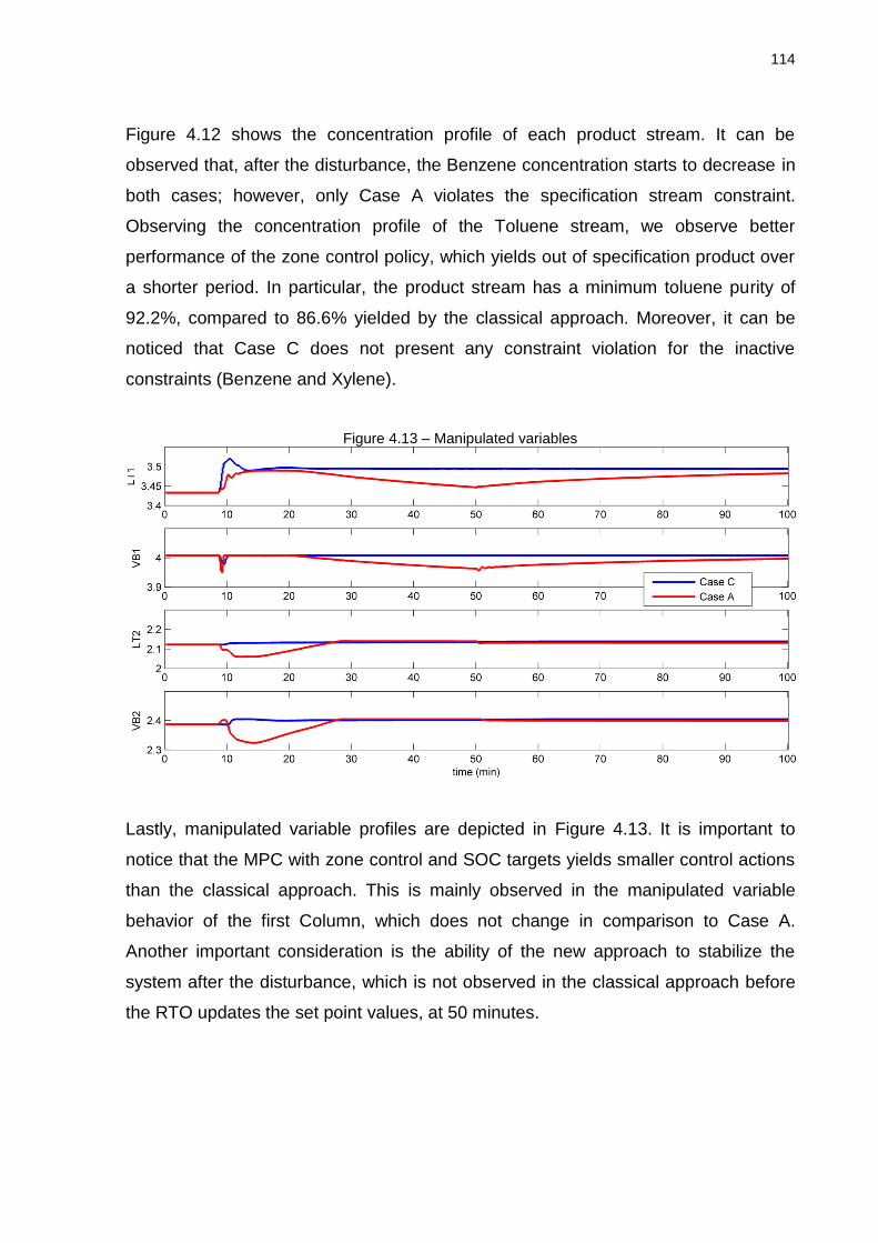
114

Figure 4.12 shows the concentration profile of each product stream. It can be

observed that, after the disturbance, the Benzene concentration starts to decrease in

both cases; however, only Case A violates the specification stream constraint.

Observing the concentration profile of the Toluene stream, we observe better

performance of the zone control policy, which yields out of specification product over

a shorter period. In particular, the product stream has a minimum toluene purity of

92.2%, compared to 86.6% yielded by the classical approach. Moreover, it can be

noticed that Case C does not present any constraint violation for the inactive

constraints (Benzene and Xylene).

Figure 4.13 – Manipulated variables

Lastly, manipulated variable profiles are depicted in Figure 4.13. It is important to

notice that the MPC with zone control and SOC targets yields smaller control actions

than the classical approach. This is mainly observed in the manipulated variable

behavior of the first Column, which does not change in comparison to Case A.

Another important consideration is the ability of the new approach to stabilize the

system after the disturbance, which is not observed in the classical approach before

the RTO updates the set point values, at 50 minutes.

115

4.5. Partial conclusions

This study presents a RTO framework with a new MPC algorithm based on zone

control and SOC variable targets. The new approach is demonstrated on two case

studies: an ammonia production plant and a multi-column distillation process. The

results at steady state and dynamic operation show better economic performance of

the new approach in comparison with classical RTO/MPC, requiring less effort from

the manipulated variables to keep the process under control. This characteristic

improves the process stability, since it requires less process changes when the RTO

is evaluated. Moreover, the zone constraint policy outperforms the classical target

approach regarding the constraints satisfaction, showing faster responses to drive

the concentration profile back to their zones or targets. These facts indicate that the

integration between RTO and SOC can be a good alternative to alleviate the

drawback of low frequency updates in RTO. Furthermore, the zone control policy is a

reliable option to handle the problem of active set changes observed in the SOC

methodology.

The concepts of SOC methodology are used in the next Chapter to evaluate different

structures of the VRD process, and then, to estimate possible improvements of

integrating RTO with SOC in this kind of process.

The main findings presented in Chapter 4 corresponds to the paper “Integrating self-

optimizing control and real-time optimization using zone control MPC”, published in

the Journal of Process Control, volume 34, pages 35-48, 2015.

116

5. Practical implementation of an RTO approach

The objective of this Chapter is to discuss the practices of the RTO implementation in

a Vapor Recompression Distillation (VRD) process. This is carried out by performing

a complete RTO cycle (in open loop), using information provided by the real plant.

As a typical rule of thumb the RTO benefits may range from 0 to 50%, which is

justified by day-to-night variations and changing market conditions. For this reason,

the RTO approach has been largely used in chemical and petrochemical industry.

Some estimates point out around 250 to 300 RTO implementations using commercial

software, not including in-house applications (DARBY et al., 2011b).

Several practical RTO implementations are reported in literature for a number of

different petrochemical processes. For instance, Sildir et al. (2013) applied the RTO

methodology to a hydrocracking process including fractionation columns. The results

showed that the control framework is able to drive the process to the optimum

condition determined by the economic optimization. Shokri et al. (2009) discussed

the applicability of the RTO methodology in refineries, showing several successful

implementations around the world and their economical benefits. Ramdial et al.

(2009) applied an RTO like framework to a petroleum field, which was able to meet

the gas market demands with increase of 7% in the condensate production. Bader

and Guesneux (2007) implemented the RTO methodology in a hydrodesulphurization

(HDS) unit with capacity to process about 870,000 ton per year, reducing in about

20% the H2 makeup and the reactor octane loss. Rotava and Zanin (2005) compared

the potential of implementing multivariate control (MVC) and RTO. The analysis of

two industrial cases studies showed that RTO is preferable, since it considered the

trade-off between energy consumption and production with a rigorous nonlinear

model. Basak et al. (2002) developed an in-house RTO solution for an industrial

crude distillation unit, increasing the profit around 8.5 million dollars per year.

Geourgiou et al. (1998) discussed the application of RTO in an ethylene production

unit, pointing out improvements in plant operations and maintenance.

117

All the papers above describe the implementation and the benefits of RTO

approaches. This is conducted in this Chapter for the VRD case study. Firstly,

Section 5.1 describes the phenomenological steady-state model used in our RTO

cycle. Then, Section 5.2 comments about the steady-state identification procedure

used to obtain the plant information. Further, the description of the parameter

estimation is performed in Section 5.3, where the plant/model adequacy is evaluated.

Section 5.4 discusses the economical improvements reached by the RTO approach.

The comparison between the implementation of RTO or MPC alone is carried out in

Section 5.5. Finally, the partial conclusions are drawn in Section 5.6.

5.1. Process description

The present section describes a mathematical model suitable for RTO

implementation on an industrial-scale depropanizer column (in Paulínea refinery

owned by Petrobras S.A.). VRD is a well-known highly integrated energy process,

widely used in the chemical industry to split close-boiling mixture, such as propylene

and propane (ANNAKOU; MIZSEY, 1995). The main characteristic of VRD process is

that additional mechanical energy is added to the overhead vapor stream by a

compressor; then this stream is used to boil up the mixture in the reboiler, reducing

the total amount of demanded energy compared to a traditional distillation scheme.

The highly interlinked structure involved in the VRD process, coupled to the

nonlinearities and the large number of equations (around 8000 in this specific case)

make the simulation particularly difficult to converge in sequential modular simulators

(AYDIN; BENALI, 2009; HEYEN; LEDENT; KALITVENTZEFF, 1994), requiring an

equation oriented approach to handle the convergence obstacles generated by this

recycle system (MEIXELL; GOCHENOUR; CHEN, 2010). In the present work the

VRD process is modeled in the software EMSO (Environment for Modeling,

Simulation and Optimization), which is an equation oriented simulator conceived and

developed in a joint effort of Brazilian universities, Petrobras and Braskem, to be a

tool for educational and industrial purposes (RODRIGUES; SOARES; SECCHI,

2010). Some features that make EMSO adequate to RTO implementation are the

118

calculation of first order derivatives via automatic differentiation, robust nonlinear

algebraic solver and modules for parameter estimation and optimization.

The schematic structure of VRD process is depicted in Figure 5.1. First, a low

molecular weight hydrocarbon mixture (mainly propylene and propane) enters the

distillation column, where high-purity propylene (99.95%) is obtained as overhead

product stream D, and propane (95%) is obtained as the main product at the bottom

stream B. The overhead stream is mixed with vapor stream from the distillate drum,

and then, it is compressed to increase its condensing temperature. After that, the

largest part of the compressor outlet stream feeds the reboiler (Fboil), while the rest

(about 10%) is condensed with cooling water (Fcool) to control the column pressure.

Subsequently, the propylene streams (hot stream) from reboiler and condenser

expand through throttle valves, returning to the distillate drum, where a portion of the

liquid is sent to the column as reflux stream (R), and the other part is stored as high

purity propylene (D).

Figure 5.1 - Schematic representation of the VRD process

The equipment in this process are modeled considering thermodynamic aspects

only, using thermodynamic properties calculated with Peng and Robinson (PR)

equation of state and predictive-SRK mixing rule (HOLDERBAUM; GMEHLING,

119

1991), which is provided by the IISE (Industrial Integrated Simulation Environment)

thermodynamic package of VRtech® company.

The main characteristics of each equipment are given below and the summary of

equipment equations is shown in Appendix G.

Distillation Tower

This equipment is modeled as a collection of individual trays (numbered from top to

bottom), which are described by rigorous mass, equilibrium, summation and heat

(MESH) equations. The column has 197 theoretical plates with feed stream at 157th

tray. The pressure profile is given by a linear approximation where the top and the

bottom pressures are set at constant values. Mass transfer aspects are included in

the model via vapor Murphree efficiencies (adjustable parameter), two for the

rectification and one for the stripping section.

Compressor

The rotary compressor is modeled using isentropic efficiency, CP , and specified

discharge pressure. The problem with this formulation is that, in the real process, the

isentropic efficiency is not a constant value, changing from different operating points.

For this reason, it is proposed to replace the constant value of CP by a function of the

product of delta pressure ( CPP ) times mass flow rate ( CPQ ). Figure 5.2 shows the

measurements of three years of process operation where it is possible to observe a

linear correlation between these variables.

120

Figure 5.2 - Measured efficiency against the product .CP CPP Q

Equation 5.1 describe the linear correlation obtained from this data and Figure 5.3

shows the comparison of the predicted and measured compressor power using the

correlation in eq.(5.1). It is worth to notice that the model is able to predict the power

consumption with small deviations.

40.5307 3.4619 .CP CP CPe Q P 5.1

Figure 5.3 - Comparison of predicted and measured power

Reboiler

The reboiler is modeled as an adiabatic countercurrent heat exchanger, in which the

temperature of the inlet streams is given by the solution of column and compressor

models. The vapor fraction of the cold outlet stream (propane to column) is set by an

adjustable parameter and the temperature of the propylene outlet stream is

121

empirically determined using plant historical data. The histogram, given in Figure 5.4

B, demonstrates that the difference of temperatures between the propylene outlet

stream and propane inlet stream is approximately constant, about 0.547°C. For this

reason, the propylene outlet temperature is set to 0.547°C higher than the propane

inlet stream.

Figure 5.4 - Historic data of the reboiler temperature profile A

B

Cooler

The model of this equipment is similar to the reboiler, but in this case the cooling

water flow rate is estimated by a function of propylene flow rate, overall heat transfer

coefficient (adjustable parameter) and the logarithmic mean temperature difference.

This formulation requires the specification of the temperature in the outlet hot stream,

which is given by analysis of the historical data. Figure 5.5 depicts the histogram of

measured temperatures in the cooler. One can see that the difference between hot

outlet stream and cooling water inlet stream temperature is almost constant at 0.05

°C. justifying the temperature of the hot outlet stream to be set 0.05 °C higher than

the measured temperature of cooling water.

122

Figure 5.5 - Historic data of the cooler temperature profile A

B

Throttle valves

The expansion valves are modeled as an adiabatic and isenthalpic process, in which

the outlet stream is in liquid-vapor equilibrium. The outlet stream pressure is set as

the measured pressure in the distillate drum.

Feedstock characteristics

Figure 5.6 shows the distribution profile of the feed stream flow rate (A) and

components concentration (B and C), in a period of three operating years. It is

important to notice that the process operates in a large range of feed conditions, but

in about 72% of times the flow rate is between 7.5 and 12 mass/time units, while the

concentration profiles distribution is similar to an uniform distribution, varying from 60

to 80% for propylene and 20 to 40% for propane.

123

Figure 5.6 - Feed stream characteristics A

B

C

Product stream characteristics

Figure 5.7 displays the distribution profile of the mass flow rate and contaminant

concentration in the overhead and bottom product streams. It may be appreciated

that the process is able to handle the disturbances in the feedstock, keeping the

contaminant concentration in the overhead stream less than its upper bound (5000

ppm), at least for 97.11% of sample times. In contrast, the contaminant concentration

in the bottom stream is greater than its upper limit (5%) in 47.50% of time, resulting in

economic loss due to large amount of propylene sent to the bottom stream.

Figure 5.7 - Products characteristics A

B

C

D

124

5.2. Steady state identification

As discussed in previous Chapters, the RTO methodology is based on steady-state

phenomenological models, requiring stationary information to update the key

parameters at each iteration. In this subsection, the steady-state identification (SSI)

method used in this work is presented.

Several different approaches of SSI have been developed in the literature, for

instance, methods based on F-like test (CAO; RHINEHART, 1995a), wavelet theory

(JIANG et al., 2003), polynomial equations (LE ROUX et al., 2008) and ARX (Auto-

Regressive with eXogenous inputs) models (RINCON; LIMA; LE ROUX, 2015).

Basically, each of these methods compute quantities from the measured states that

are compared to critical values; if this comparison satisfies a determined condition

the process is considered to be in steady-state. The problem associated with all

these approaches is the need for adequate tuning, which relies on specific

measurements characteristics such as noise and frequency. Rincon and coworkers

(2015) compared different approaches and found that, after proper tuning, the F-like

test presents similar levels of performance than more complex methods, which

motivated its application in our case study.

The Cao and Rhinehart (1995) SSI method is an F-like test, which basically

compares two variance estimates computed in different ways. First of all, the

measured state ( iX ) is filtered by an exponential filter, using 1 as smoothing factor

(eq.(5.2)). Then the filtered value ( ,f iX ) is used to compute the first variance estimate

(2

,f i ) in eq.(5.3), while the second variance estimate (2

,f i ) is calculated only based

on the measured states ( iX and 1iX ), eq.(5.4). After that, the ratio between these two

variance estimates is used in the SSI index iR (see, eq.(5.5)), which is finally

compared to a critical value crR . If iR is less than crR the process is considered at

steady-state. Otherwise, the process is assumed in transient regime.

, 1 1 , 11f i i f iX X X (5.2)

125

2

2 2

, 2 , 1 2 , 11f i i f i f iX X (5.3)

22 2

, 3 1 3 , 11f i i i f iX X (5.4)

2

1 ,

2

,

2 f i

i

f i

R

(5.5)

Seven measured variables are chosen to detect the process steady-state: three

stream flow rates (feed, overhead and bottom product) and four concentration

measurements (propylene composition of feed and bottom product and propane

composition in feed and overhead streams). The smoothing factors 1 , 2 and 3

are determined by visual inspection, resulting in 0.7, 0.05 and 0.006 respectively,

while the crR value is set equal to 2. Representative steady-states are selected as

information for the parameter estimation performed in the following subsection.

5.3. Parameter estimation

In this section the Rotational Discrimination (RD) methodology is applied to the VRD

case study, using real information from the propylene production unit of REPLAN

refinery of Petrobras. The tests are conducted in the software EMSO by using a RD

routine written in C++ language (see the algorithm depicted in Figure 3.2).

Firstly, the RD routine is tested in a small case study to evaluate the correctness of

its implementation, where these outcomes are compared with a classical weighted

least squares (LSq) approach already available in the EMSO software package. The

case study chosen in this test is the Williams Otto chemical reactor, previously

described in Section 2.3 of this thesis. Basically, this process is composed of a CSTR

reactor, which is fed with components A and B to produce the products P and E, and

a waste byproduct G.

126

Five different operating points are simulated with the original parameters values

(Region 1 of Table 2.1). Then, the obtained values of P and E concentrations are

used as measured variables for the parameter estimation problem, which is solved

with RD and LSq routines. Both methods are set with the same termination criteria

tolerance (1e-9).

Table 5.1 summarizes the results obtained by both approaches, where the values of

the objective function and parameters are compared. It is worth to observe that RD

approach presents smaller values of the objective function, but with a larger number

of objective function evaluations than the LSq method. The difference in the number

of objective functions evaluations does not necessarily represent a significant

discrepancy in computational time, which is 0.108 and 0.056 seconds for RD and

LSq respectively, at least for this small case study.

Another important remark about the RD results is related to the parameters values.

One may notice that RD approach presents smaller parameter deviations from the

initial values in comparison to LSq. This fact indicates that the algorithm is able to

perform what it is aimed to do, which is to minimize the objective function without

increasing the parameter inflation resulting from identifiability issues.

Table 5.1 - Summary of the parameter estimation results for the WO case study

Parameter values Parameter deviation

from the initial value

Initial value LSq RD LSq

RD *ObF value ----- 2.85831e-04 2.80622e-04 ----- -----

*ObF evaluations 0 22 69 ----- -----

1ηp 1.6e06 5.2544e06 1.4081e06 228.40% -11.99%

2ηp 7.2e08 2.2928e09 7.8325e08 218.45% 8.78%

3ηp 2.6e12 1.9400e13 2.2481e12 646.14% -13.53%

1Ea 6600 7154 6646 8.39% 0.70%

2Ea 8300 8109 8271 -2.30% -0.35%

3Ea 11000 11275 11051 2.50% 0.47% *ObF: objective function

The results of the first case study show that the RD algorithm written in C++ is well

implemented. The next step is to conduct the parameter estimation in the VRD case

study using the representative steady-state found by the procedure described in

Section 5.2.

127

In this parameter estimation problem, 6 model parameters are used to fit the process

data and other 5 measured states are set as "parameters" in order to be

reconciliated; the detailed list of parameters can be appreciated in Table 5.2. In

addition, 9 states are set at their measured values and 23 measured states are used

in the objective function (see Table 5.3). The standard deviations used in the

objective function are also computed from the historical data and displayed in Table

5.3.

Table 5.2 - Parameters used in the VRD estimation

Parameter type

Description Unit Lower bound

Upper bound

Model parameter

Column - Murphree efficiency section 1 ------ 0.5 1.2 Column - Murphree efficiency section 2 ------ 0.5 1.2 Column - Murphree efficiency section 3 ------ 0.5 1.0 Column - heat exchanged with the environment W 0 5000 Cooler - overall heat transfer coefficient W/m

2K 200 1000

Reboiler - vapor fraction of the outlet propane stream ------ 0.25 1.0

Reconciliated data

Propylene composition in feed stream %-mol 20 90 Feed stream flow rate mass/time 6.4e3 1.5e4 Reflux flow rate mass/time 6.4e4 1.1e5 Bottom product flow rate mass/time 2.6e2 5.1e3 Column top pressure kgf/cm

2 8 12

The parameter estimation algorithm is executed and converges in about 17 minutes,

which is a small period when compared to the process settling time of 10-12 hours.

Figure 5.8 shows the temperature profile of the column after the parameter

estimation. It can be seen that the prediction has a good agreement with the

measured values.

Figure 5.8 - Temperature profile of VRD column after parameter estimation

128

Table 5.3 displays the values of the measured and predicted states, organized by

equipment. One can observe that the deviation between the process and the model

is not greater than 5% for most of the measured states. The highest deviation is

obtained in the propane concentration at the overhead stream, which is not an issue

since the observed deviation is still smaller than measurement variance (559ppm2

against 900 ppm2).

Four out of six parameters used in the parameter estimation reach their limits. The

three Murphree efficiencies are adjusted to their upper bounds, probably to

compensate possible inaccuracies of the thermodynamic model. Moreover, the vapor

fraction at the reboiler outlet stream (vapor to the column) reaches its lowest value.

In general, the results demonstrate that the model is able to reproduce the process

behavior and can be applied to the RTO algorithm. The next section presents the

economic optimization of this updated model, in order to evaluate the economical

benefits related to the RTO implementation.

continue...

Table 5.3 - Summary of the parameter estimation results for the VRD process case study

Process variable Unit Measured

value Std Predicted

value Deviation

%

Feed s

trea

m Temperature* °C 24.96 0.03 24.96 ------

Pressure* kgf/cm² 11.49 0.01 11.49 ------

Flow rate** mass/time 7.32 0.26 7.19 -1.72

Propylene concentration** %-mol 78.03 0.15 77.26 -0.98

Propane concentration** %-mol 22.00 0.14 22.73 3.32

Ethane concentration* ppm 0.13 0.14 15.84 ------

Com

pre

ssor Suction temperature °C 19.20 0.03 18.27 -4.85

Discharge temperature °C 44.88 0.06 46.77 4.22

Suction Pressure kgf/cm² 10.14 0.00 9.92 -2.16

Discharge Pressure* kgf/cm² 16.17 0.02 16.17 ------

Power MW 3.51 0.01 3.36 -4.12

129

...

Process variable Unit Measured

value std

Predicted value

Deviation %

Coole

r

Propylene inlet temperature °C 44.88 0.00 46.77 4.22

Cooling water inlet temperature* °C 25.90 0.48 25.90 ------ Cooling water outlet temperature** °C 30.55 0.59 30.54 -0.06

flooding level* % 50.20 1.29 50.20 ------

Cooling water flow rate mass/time ------ ------- 195.32 ------

Propylene outlet temperature* °C 25.84 0.49 26.05 0.82

Propylene flow rate** mass/time 10.85 0.52 10.28 -5.22

Bott

om

pro

duct Flow rate** mass/time 1.73 0.40 1.77 2.45

Temperature °C 30.88 0.12 30.70 -0.59

Propylene concentration** %-mol 4.42 0.43 4.64 4.89

Overh

ead

pro

duct Temperature °C 30.40 0.04 30.35 -0.16

Propane concentration** ppm 312.32 30.28 871 178.85

Flow rate** mass/time 5.66 0.31 5.43 -4.11

Reflux

str

eam

Pressure* kgf/cm² 15.89 0.01 15.90 ------

Flow rate** mass/time 92.59 0.75 93.43 0.91

Reflux

dru

m

Pressure* kgf/cm² 13.45 0.01 13.45 ------

Outlet stream temperature °C 30.29 0.03 30.35 0.20

** measured states used in the estimation objective function

* measured states set in the model

Tow

er

Top pressure** kgf/cm² 10.04 0.01 9.92 -1.19

Tray 17th** °C 18.83 0.02 18.73 -0.54

Tray 35th** °C 19.39 0.02 19.24 -0.77

Tray 51st** °C 19.67 0.02 19.70 0.13

Tray 69th** °C 20.15 0.02 20.22 0.34

Tray 85th** °C 20.60 0.02 20.69 0.46

Tray 119th** °C 21.63 0.02 21.78 0.73

Tray 137th** °C 22.32 0.02 22.47 0.66

Tray 153rd** °C 23.01 0.02 23.23 0.94

Tray 171st** °C 24.30 0.07 24.42 0.50

V stream temperature °C 30.56 0.06 30.73 0.57

Bottom pressure** kgf/cm² 11.37 0.01 11.36 -0.04

Rebo

iler Propylene inlet temperature °C 44.88 0.00 46.77 4.22

Propane outlet temperature** °C 30.56 0.06 30.73 0.57

Propylene outlet temperature °C 30.94 0.05 31.15 0.71

Propylene flow rate** mass/time 88.49 0.37 88.73 0.27

130

5.4. Optimization

With the updated model at hand, it is possible to optimize the model according to the

economic objective function. Essentially, the main objective of this plant is to produce

high purity propylene at overhead stream, which is sold to a polymer industry at a

higher price compared to the bottom stream (propane incorporated in LPG).

Therefore, the economic objective function is composed of the operating cost given

by the sum of profits (overhead and bottom products) minus the sum of utilities

(compressor energy and cooling water) and feedstock cost.

The problem of the above objective function formulation is that the feedstock stream

is an intermediate stream, which does not have an assigned market price, and

cannot be compared to the cost of other streams. An alternative to circumvent this is

to employ a wide-plant approach and to optimize several units at the same time, in

which all inlet and outlet streams have assigned market prices. However, this

approach is not efficient because it is almost impossible that all units achieve steady-

states at the same time in order to be optimized (RINALDO; UNGAR, 2000).

Another possibility is to optimize the process using decomposition techniques, to

obtain fictitious prices (shadow prices) for the intermediate streams, which are then

used to optimize each unit at a time (CONEJO et al., 2006; GUIGNARD, 2003). The

implementation of decompositions techniques in the propylene production unit was

previously studied in our research group, resulting in the shadow price used in this

thesis; the complete study can be found in (ACEVEDO et al., 2015). The list of prices

used in the VRD case is displayed in Table 5.4.

Table 5.4 - Price list

Cost component Unit Value

Feed stream currency/mass 397.25 Overhead stream currency/mass 893.86 Bottom stream currency/mass 229.08 Compressor energy currency/MWh 19.92 Cooling water currency/mass 0.013

Due to current problems found in the solver implementation of the EMSO

environment, it is impossible to solve large scale problems by an equation oriented

optimization approach. Therefore, the economic optimization problem is conducted

131

using a derivative-free approach (Nelder-Mead method) in the reduced space of this

problem.

Originally, the VRD process has two degrees of freedom to be optimized that are

chosen to be one internal flow rate (reflux stream) and the bottom stream flow rate.

The constraints for the products concentration are handled as 1 penalty functions

added to the objective function and the solver is tuned with relative and absolute

accuracy set at 10-8. With this tuning, the problem converges after 101 iterations with

191 objective function evaluations, in approximately 5 min.

Table 5.5 summarizes the economical gains obtained by the optimization, where it is

displayed the costs computed at the current operating point and the optimal solution.

It is important to notice that the utility cost is not significant with respect to the total

profit (approximately 0.8%); which is different from traditional distillation columns

schemes without energy integration. Furthermore, the optimization outcomes show

that it is possible to reduce the utility cost and also to increase the production of the

most valuable product (propylene), improving the total profit in 2.98% that represents

saves of around 2 million dollars per year.

Table 5.5 - Summary of the economic optimization result (cost components)

Unit Current Optimal solution Deviation %

Total profit

currency/ time

9073.87 9352.51 2.98%

Feed cost 2856.23 2856.23 0.00%

Overhead profit 4847.84 4934.12 1.75%

Bottom product profit 404.66 382.57 -5.78%

Compressor cost 67.04 60.76 -9.37%

Cooling water cost 2.59 1.62 -37.57%

The values of the most relevant process variables, before and after optimization, are

listed in Table 5.6. It can be seen that the internal flow rates (reflux, reboiler and

compressor) are significantly reduced to decrease the utility costs. However, as the

utility costs are rather negligible in comparison to the total profit, the optimization

tends to increase the amount of overhead product until the product concentrations

achieve their upper and lower bound in the overhead and bottom streams.

132

Table 5.6 - Summary of the economic optimization result (process variables)

Variable Unit Current Optimal solution Deviation %

Distillate Flow mass/time 5.43 5.52 1,66%

Distillate concentration ppm 870.92 5000.00 474,10%

Bottom Flow mass/time 1.77 1.67 -5,65%

Bottom concentration %-mol 4.64 0.30 -93,53%

Reflux Flow mass/time 93.43 80.42 -13,92%

Reboiler Flow mass/time 88.73 77.03 -13,19%

Compressor Flow mass/time 99.01 86.48 -12,66%

Actually, the optimization raises the column temperature (about 0.60ºC per tray) in

order to propel more propylene to the column top, as may be observed in Figure 5.9.

This behavior also sends more propane to the overhead stream, achieving its upper

bound of 5000ppm.

Figure 5.9 - Optimized temperature profile

5.5. Control structure

Darby et al. (2011) pointed out the importance to compare the benefits of RTO to

those than can be obtained from MPC or PID alone. This evaluation is carried out in

the present section.

In the previous section, the economical benefits of RTO are demonstrated, and it can

be seen that due to heat integration provided by the VRD process, the utilities costs

are almost irrelevant with respect to the total profit. As a consequence, the process

optimization tends to increase the overhead flow rate until the propane concentration

133

reaches its upper bound (5000ppm), while the propylene concentration reaches its

lowest value in the bottom stream (0.3%mol).

That characteristic motivates the control of both concentrations (at their bounds) to

obtaining the maximum profit at any operating point, without need of an RTO.

However, the “dual” control (control of two products composition) is known to be

difficult to be implemented due to the strong interactions (JOGWAR; DAOUTIDIS,

2009; MUHRER; COLLURA; LUYBEN, 1990; SKOGESTAD; MORARI, 1987;

SKOGESTAD, 2000), so the implementation of an MPC with a fixed set point using

both concentrations as controlled variables may be impractical.

A possible alternative could be to control the propane concentration in the overhead

stream together with another measured state, which preferentially does not change

its value for different disturbances. Table 5.7 shows the optimal values of several

measured variables, considering disturbances in flow rate and composition of feed

stream. It can be seen that all variables change their values in comparison to the

nominal state, with exception of the products concentrations.

Table 5.7 - Optimal values for different disturbances

Variable Unit Nominal

value Dist1 Dist2 Dist3 Dist3**

Feed flow rate mass/time 7.19 7.55 7.91 7.19 7.19 Feed propylene composition

%-mol 77.26 77.26 77.26 73.40 69.54

R mass/time 80.42 84.39 88.35 77.07 73.69

Fboil mass/time 77.03 81.03 85.04 73.61 70.17

D mass/time 5.52 5.80 6.07 5.23 4.95

B mass/time 1.67 1.76 1.84 1.96 2.24 Overhead propylene composition

%-mol 5000 5000 5000 5000 5000

Bottom propylene composition

%-mol 0.30 0.30 0.30 0.30 0.30

R/Feed ------ 11.18 11.17 11.17 10.71 10.24

Fboil/Feed ------ 10.71 10.73 10.75 10.23 9.76

R/D ------ 14.56 14.55 14.55 14.72 14.89

D/Feed ------ 0.77 0.77 0.77 0.73 0.69

B/Feed ------ 0.23 0.23 0.23 0.27 0.31

** Disturbance

The integration between RTO and SOC is discussed in Chapter 4. That study

inspires the proposition of a pair of controlled variables for the VRD process, one

134

would be the propane concentration at overhead stream and the other an artificial

self-optimizing control variable made-up of a linear combination of the overhead (D)

and bottom (B) streams flow rates and of the ratio Feed

Fboil . The SOC variable is

calculated in accordance to the Null Space method (ALSTAD; SKOGESTAD, 2007),

with optimal sensitivities computed by finite differences at the nominal point. Equation

5.6 presents the new pair of controlled variables.

,1

2 0.10701 0.2962 0.9491

D propy

boil

c x

Fc D B

Feed

(5.6)

To evaluate the performance of the proposed alternative, an experiment is conducted

with disturbances of 10% in the feed composition and feed flow rate, employing 1c

and 2c as controlled variables. The results show that the profit loss that can be

attributed to the control of both variables is small, about 0.09% of the optimal profit.

This outcome is an important indication that the optimum control of the VRD process

using an RTO with SOC approach may yield excellent results, since the SOC is able

to handle small disturbances and the RTO can manage larger ones.

For sure, the previous analysis is not conclusive and dynamic experiments need to

be conducted to draw a general conclusion about the ideal VRD control structure.

However, these experiments are not in the scope of the present thesis and are to be

considered for future works.


In this Chapter the practical aspects of RTO implementation in a VRD unit are

discussed. First of all, the phenomenological model is presented using process data

to determine some relevant fixed parameters. After that, the steady-state

identification method is presented, and then, the model parameters are estimated by

the Rotational Discrimination method. The parameter estimation outcomes show that

the model is flexible enough to represent the process data with small deviations and

135

can be successfully used in the RTO cycle. The economical optimization is

conducted by using the operational cost as objective function, resulting in a profit

improvement of 2.98%, equivalent to 2 million dollars per year. Finally, the

improvements obtained by the RTO approach are compared to the ones obtained by

the MPC alone. Although the dual control of both products composition is enough to

keep the process at the economical optimum, this control strategy may have poor

results, due to strong interaction between the controlled variables (SKOGESTAD;

MORARI, 1987). This fact motivates the proposition of a new control structure using

SOC variables. Preliminary results show that the proposed control approach (RTO

plus SOC) could lead to small profit losses and would be a good alternative to the

VRD control. However, more experiments need to be conducted to guarantee the

superiority of RTO plus SOC in comparison to MPC alone. Moreover, other methods

to calculate SOC variables should also be considered that include implementation

errors, for instance.

136

6. General Conclusions and Future Works

In the thesis the Real Time Optimization methodology applied to chemical processes

has been studied. This is an attractive alternative to control many process systems,

because it has a high acceptance among process operators. Although the large

number of RTO implementations in industry, its benefits are not always self-evident

because this method has some drawbacks that need to be reduced for proper

operation, namely: plant/model mismatch, non-identifiability problems and low

frequency of set points updates. Each of these problems was separately analyzed

and alternatives were proposed to mitigate their influence on the RTO cycle, resulting

in an improved RTO framework. Then, the proposed approaches were successfully

applied to an industrial case of study.

The main conclusions of this thesis may be summed up as following:

a) The comparison between RTO strategies shows that the classical RTO

method (Model Parameter Adaptation) may be reliable, provided that a flexible

model to represent process topology, a parameter estimation method suitable

to handle process noise characteristics, lack of model identifiability and a

method to improve the quality of measurements (Dual methodology) are used

in combination.

b) The evaluation of the parameter estimation methodologies demonstrates that

the Rotational Discrimination (RD) method is likely the most appropriate

among the evaluated methods to be used in a RTO-like framework, because it

presents the best prediction capacity and robustness, with reasonable

computational time, in the examples that studied in this thesis.

c) The results obtained in the development of the MPC integrating Self-

Optimizing Control (SOC) and RTO point out that the combination of these

methodologies may be a good alternative to alleviate the inconvenience of low

frequency set point updates in RTO. Moreover, the zone control policy is a

consistent option to handle the problem of active set point changes observed

in the SOC methodology.

137

d) The RTO implementation in an industrial case study shows that it is possible

to increase the VRD process profit in 2.98%, which is equivalent to saves

around 2 million dollars per year. Moreover, the comparison between the

control structures shows that the integrated approach between RTO and SOC

may be an interesting alternative for this process.

e) One of the main drawbacks in the RTO methodology is that it is necessary that

the process be at steady-state. This limits the frequency of application of the

estimation, re-optimization cycle, and it depends solely on the control

performance, the characteristics of perturbations of the system and on the

dynamics of the process.

Some of the drawbacks in RTO were studied in detail in this thesis, but some are

inherent to the methodology. In this sense, it would be interesting to provide some

suggestions for future works:

a) The Rotational Discrimination method may be extended using redescending

estimators to integrate parameter estimation and reconciliation modules. This

approach would be able to handle simultaneously, and in a robust way, gross

errors and identifiability problems.

b) It is necessary to analyze other methods to compute SOC variables including

measurement errors, and then integrate these methods to the MPC developed

in the present work.

c) It would be interesting to develop a general alternative to handle both

problems related with changes in the active set (see Chapter 4). One

possibility is to employ only unconstrained variables as controlled variables

and calculate the optimum sensitivity matrix via surface response methods,

similar to the work of Ye et al. (2013).

d) Development of an MPC integrating RTO and SOC with for example using

infinity horizon to guarantee Lyapunov stability.

138

f) The dynamic comparison among different control structures for the VRD case

study including possible SOC variables is necessary to evaluate economic

and stability benefits of RTO methodology in this process.

g) The identification of continuous processes by steady-state models is a difficult

task, mainly because the information used in the parameter estimation is

punctual and the time is crucial. An alternative to handle this problem is to use

a dynamic model to take advantage of measurements in the transient period,

improving the parameter estimation. This approach would be similar to the

Dynamic Real Time Optimization (DRTO) with the difference that the

economic optimization could be performed by the steady-state model, such as

done in the classic RTO, which would reduce at least one dynamic

optimization problem.

139

REFERENCES

ACEVEDO, A. M.; GRACIANO, J.E.A.; LIPORACE, F.; LE ROUX, G.A.C.

Decomposition Techniques for the Real-time Optimization of a Propylene

Production Unit25th European Symposium on Computer Aided Process

Engineering. Copenhagen: Elsevier, 2015

ALSTAD, V.; SKOGESTAD, S. Null Space Method for Selecting Optimal

Measurement Combinations as Controlled Variables. Industrial & Engineering

Chemistry Research, v. 46, n. 3, p. 846–853, jan. 2007.

ALSTAD, V.; SKOGESTAD, S.; HORI, E. S. Optimal measurement combinations as

controlled variables. Journal of Process Control, v. 19, n. 1, p. 138–148, jan. 2009.

ANNAKOU, O.; MIZSEY, P. Rigorous investigation of heat pump assisted distillation.

Heat Recov. Syst. CHP, v. 15, n. 3, p. 241, abr. 1995.

ARORA, N.; BIEGLER, L. T. Redescending estimators for data reconciliation and

parameter estimation. Comput. Chem. Eng., v. 25, n. 11-12, p. 1585, nov. 2001.

AYDIN, B.; BENALI, M. Simulation and optimization of depropanizer, C3-splitter

and debutanizerSpring Meeting & 5th Global Congress on Process Safety. Tampa:

2009

BADER, J.-M.; GUESNEUX, S. Use real-time optimization for low-sulfur gasoline

production. Hydrocarbon processing, v. 86, n. 2, 2007.

BAMBERGER, W.; ISERMANN, R. Adaptive on-line steady-state optimization of slow

dynamic processes. Automatica, v. 14, n. 3, p. 223–230, may 1978.

BARD, Y. Comparison of Gradient Methods for the Solution of Nonlinear Parameter

Estimation Problems. SIAM Journal on Numerical Analysis, v. 7, n. 1, p. 157–186,

mar. 1970.

BARD, Y. Nonlinear parameter estimation. New York: Academic Press, 1974.

BARD, Y.; LAPIDUS, L. Nonlinear System Identification. Industrial & Engineering

Chemistry Fundamentals, v. 9, n. 4, p. 628–633, nov. 1970.

BASAK, K.; ABHILASH, K.B.; GANGULY, S.; SARAF, D.N. On-Line Optimization of a

Crude Distillation Unit with Constraints on Product Properties. Ind. Eng. Chem. Res.,

v. 41, n. 6, p. 1557, mar. 2002.

BELLMAN, R.; ÅSTRÖM, K. J. On structural identifiability. Mathematical

Biosciences, v. 7, n. 3-4, p. 329–339, abr. 1970.

BEN-ZVI, A. Reparameterization of inestimable systems with applications to chemical

and biochemical reactor systems. AIChE Journal, v. 54, n. 5, p. 1270–1281, maio

140

2008.

BERTSEKAS, D. P.; NEDIÂC, A.; OZDAGLAR, A. E. Convex analysis and

optimization. e.1. ed. Belmont: Athena Scientific, 2003.

BIEGLER, L. T.; DAMIANO, J. J.; BLAU, G. E. Nonlinear parameter estimation: A

case study comparison. AIChE Journal, v. 32, n. 1, p. 29–45, jan. 1986.

BIEGLER, L. T.; GROSSMANN, I. E.; WESTERBERG, A. W. A note on

approximation techniques used for process optimization. Computers & Chemical

Engineering, v. 9, n. 2, p. 201–206, 1985.

BRDYS, M. A.; TATJEWSKI, P. Iterative Algorithms for Multilayer Optimization

Control. London: Imperial College Press, 2005.

BUNIN, G. A.; FRANÇOIS, G.; BONVIN, D. Performance of Real-Time Optimization

Schemes – I. Sufficient Conditions for Feasibility and Optimality. Computer and

Chemical Engineering (subimitted), v. submitted, 2013a.

BUNIN, G. A.; FRANÇOIS, G.; BONVIN, D. Performance of Real-Time Optimization

Schemes – II. Implementation Issues. Computer and Chemical Engineering

(subimitted), v. submitted, 2013b.

BUNIN, G. A.; FRANÇOIS, G.; BONVIN, D. Sufficient Conditions for Feasibility and

Optimality of Real-Time Optimization Schemes - I. Theoretical Foundations. 12 ago.

2013c.

BUNIN, G. A.; FRANÇOIS, G.; BONVIN, D. Sufficient Conditions for Feasibility and

Optimality of Real-Time Optimization Schemes - II. Implementation Issues. p. 56, 12

ago. 2013d.

BUNIN, G. A.; FRANÇOIS, G.; BONVIN, D. From Discrete Measurements to

Bounded Gradient Estimates: A Look at Some Regularizing Structures. Industrial &

Engineering Chemistry Research, v. 52, n. 35, p. 12500–12513, 4 set. 2013e.

CAO, S.; RHINEHART, R. R. An efficient method for on-line identification of steady

state. Journal of Process Control, v. 5, n. 6, p. 363–374, 1995a.

CAO, S.; RHINEHART, R. R. An efficient method for on-line identification of steady

state. Journal of Process Control, v. 5, n. 6, p. 363–374, dez. 1995b.

CAO, Y. Direct and indirect gradient control for static optimisation. International

Journal of Automation and Computing, v. 2, n. 1, p. 60–66, jul. 2005.

CHU, Y.; HUANG, Z.; HAHN, J. Global Sensitivity Analysis Procedure Accounting for

Effect of Available Experimental Data. Industrial & Engineering Chemistry

Research, v. 50, n. 3, p. 1294–1304, 2 fev. 2011.

CONEJO, A. J. et al. Decomposition techniques in mathematical programming:

engineering and science applications. [s.l.] Springer Science & Business Media,

141

2006.

DARBY, M. L.; NIKOLAOU, M.; JONES, J.; NICHOLSON, D. RTO: An overview and

assessment of current practice. J. Process Contr., v. 21, n. 6, p. 874, jul. 2011a.

DARBY, M. L. et al. RTO: An overview and assessment of current practice. Journal

of Process Control, v. 21, n. 6, p. 874–884, jul. 2011b.

DE ARAÚJO, A. C. B.; GOVATSMARK, M.; SKOGESTAD, S. Application of

plantwide control to the HDA process. I—steady-state optimization and self-

optimizing control. Control Engineering Practice, v. 15, n. 10, p. 1222–1237, out.

2007.

EFRON, B. Biased versus unbiased estimation. Advances in Mathematics, v. 16, n.

3, p. 259–277, jun. 1975.

ENGELL, S. Feedback control for optimal process operation. Journal of Process

Control, v. 17, n. 3, p. 203–219, mar. 2007.

FARISS, R. H.; LAW, V. H. An efficient computational technique for generalized

application of maximum likelihood to improve correlation of experimental data.

Computers & Chemical Engineering, v. 3, n. 1-4, p. 95–104, jan. 1979.

FORBES, J. F.; MARLIN, T. E. Model Accuracy for Economic Optimizing Controllers:

The Bias Update Case. Industrial & Engineering Chemistry Research, v. 33, n. 8,

p. 1919–1929, ago. 1994.

FORBES, J. F.; MARLIN, T. E.; MACGREGOR, J. F. Model adequacy requirements

for optimizing plant operations. Comput. Chem. Eng., v. 18, n. 6, p. 497, jun. 1994.

GEORGIOU, A.; SAPRE, A.V.; TAYLOR, P.; GALLOWAY, R.E; CASEY, L.K.

Ethylene optimization system reaps operations and maintenance benefits. Oil and

Gas Journal, v. 96, n. 10, 1998.

GONZÁLEZ, A. H.; ODLOAK, D. A stable MPC with zone control. Journal of

Process Control, v. 19, n. 1, p. 110–122, jan. 2009.

GRACIANO, J. E.; MENDOZA, D. F.; LE ROUX, G. A. C. Performance comparison of

parameter estimation techniques for unidentifiable models. Computers & Chemical

Engineering, v. 64, p. 24–40, may 2014.

GUIGNARD, M. Lagrangean relaxation. Top, v. 11, n. 2, p. 151–200, 2003.

HAAKER, M. P. R.; VERHEIJEN, P. J. T. Local and Global Sensitivity Analysis for a

Reactor Design with Parameter Uncertainty. Chemical Engineering Research and

Design, v. 82, n. 5, p. 591–598, may 2004.

HALVORSEN, I. J. et al. Optimal Selection of Controlled Variables †. Industrial &

Engineering Chemistry Research, v. 42, n. 14, p. 3273–3284, jul. 2003.

HANGOS, K.; CAMERON, I. Process system engineering : process modeling

142

and modeling analysis. London: Academic Press, 2001.

HEYEN, G.; LEDENT, T.; KALITVENTZEFF, B. A modular package for simultaneous

calculation of complex interlinked separation processes. Comput. Chem. Eng., v.

18, p. S69, jan. 1994.

HOLDERBAUM, T.; GMEHLING, J. PSRK: A Group Contribution Equation of State

Based on UNIFAC. Fluid Phase Equilibria, v. 70, n. 2-3, p. 251–265, dez. 1991.

HU, W. et al. Local self-optimizing control of constrained processes. Journal of

Process Control, v. 22, n. 2, p. 488–493, fev. 2012.

JASCHKE, J.; SKOGESTAD, S. Using Process Data for Finding Self-optimizing

Controlled VariablesInternational Symposium on Dynamics and Control of Process

Systems. Anais...Mumbai: 2013

JÄSCHKE, J.; SKOGESTAD, S. NCO tracking and self-optimizing control in the

context of real-time optimization. Journal of Process Control, v. 21, n. 10, p. 1407–

1416, dez. 2011.

JIANG, T. et al. Application of steady-state detection method based on wavelet

transform. Computers & Chemical Engineering, v. 27, n. 4, p. 569–578, abr. 2003.

JOGWAR, S. S.; DAOUTIDIS, P. Dynamics and control of vapor recompression

distillation. Journal of Process Control, v. 19, n. 10, p. 1737–1750, dez. 2009.

JOSE, R. A.; UNGAR, L. H. Pricing interprocess streams using slack auctions.

AIChE Journal, v. 46, n. 3, p. 575–587, mar. 2000.

KARIWALA, V.; CAO, Y.; JANARDHANAN, S. Local Self-Optimizing Control with

Average Loss Minimization. Industrial & Engineering Chemistry Research, v. 47,

n. 4, p. 1150–1158, fev. 2008.

KEESMAN, K. J.; SPANJERS, H.; STRATEN, G. VAN. Analysis of endogenous

process behavior in activated sludge. Biotechnology and Bioengineering, v. 57, n.

2, p. 155–163, 1998.

LARSSON, T. et al. Self-Optimizing Control of a Large-Scale Plant: The Tennessee

Eastman Process. Industrial & Engineering Chemistry Research, v. 40, n. 22, p.

4889–4901, out. 2001.

LE ROUX, G. A. C. Strategie d’identification de modeles algebro-diferentiels.

Application aux systemes reactionnels complexes. [s.l.] Institut national

polytechnique de tolouse, 1995.

LE ROUX, G. A. C. et al. Improving steady-state identification. Proceedings of the

18th European Symposium on Computer Aided Process Engineering –

ESCAPE 18, v. 25, p. 459–464, 2008.

LEER, R. B. Self-optimizing control structures for active constraint regions of a

143

sequence of distillation columns. [s.l.] Norwegian University of Science and

Technology, 2012.

LERSBAMRUNGSUK, V. et al. Control structure design for optimal operation of heat

exchanger networks. AIChE Journal, v. 54, n. 1, p. 150–162, jan. 2008.

LI, R.; HENSON, M. A.; KURTZ, M. J. Selection of Model Parameters for Off-Line

Parameter Estimation. IEEE Transactions on Control Systems Technology, v. 12,

n. 3, p. 402–412, maio 2004.

LUBANSKY, A. S. et al. A general method of computing the derivative of

experimental data. AIChE Journal, v. 52, n. 1, p. 323–332, jan. 2006.

LUND, B. F.; FOSS, B. A. Parameter ranking by orthogonalization—Applied to

nonlinear mechanistic models. Automatica, v. 44, n. 1, p. 278–281, jan. 2008.

MAEDER, U.; BORRELLI, F.; MORARI, M. Linear offset-free Model Predictive

Control. Automatica, v. 45, n. 10, p. 2214–2222, out. 2009.

MANSOUR, M.; ELLIS, J. E. Comparison of methods for estimating real process

derivatives in on-line optimization. Applied Mathematical Modelling, v. 27, n. 4, p.

275–291, apr. 2003.

MANUM, H.; SKOGESTAD, S. Self-optimizing control with active set changes.

Journal of Process Control, v. 22, n. 5, p. 873–883, jun. 2012.

MARCHETTI, A. Modifier-Adaptation Methodology for Real-Time Optimization.

[s.l.] ÉCOLE POLYTECHNIQUE FÉDÉRALE DE LAUSANNE, 2009.

MARCHETTI, A.; CHACHUAT, B.; BONVIN, D. Modifier-Adaptation Methodology for

Real-Time Optimization. Industrial & Engineering Chemistry Research, v. 48, n.

13, p. 6022–6033, jul. 2009.

MARQUARDT, D. W. An Algorithm for Least-Squares Estimation of Nonlinear

Parameters. Quarterly of Applied Mathematics, v. 11, n. 2, p. 431–411, 1963.

MARQUARDT, D. W. Generalized Inverses, Ridge Regression, Biased Linear

Estimation, and Nonlinear Estimation. Technometrics, v. 12, n. 3, p. 591–612, ago.

1970.

MCLEAN, K. A. P.; MCAULEY, K. B. Mathematical modelling of chemical processes-

obtaining the best model predictions and parameter estimates using identifiability and

estimability procedures. The Canadian Journal of Chemical Engineering, v. 90, n.

2, p. 351–366, 17 abr. 2012.

MEIXELL, M. D.; GOCHENOUR, B.; CHEN, C.-C. Chapter 3 – Industrial Applications

of Plant-Wide Equation-Oriented Process Modeling—2010. In: SUNDMACHE, K.

(Ed.). . Adv. Chem. Eng. Burlington: Elsevier, 2010. p. 152.

MIAO, H. et al. On identifiability of nonlinear ode models and applications in viral

144

dynamics. SIAM review. Society for Industrial and Applied Mathematics, v. 53, n.

1, p. 3–39, 1 jan. 2011.

MILETIC, I. P.; MARLIN, T. E. On-line Statistical Results Analysis in Real-Time

Operations Optimization. Industrial & Engineering Chemistry Research, v. 37, n.

9, p. 3670–3684, set. 1998.

MUHRER, C. A.; COLLURA, M. A.; LUYBEN, W. L. Control of vapor recompression

distillation columns. Ind. Eng. Chem. Res., v. 29, n. 1, p. 59, jan. 1990.

NGUYEN, V. V.; WOOD, E. F. Review and Unification of Linear Identifiability

Concepts. SIAM Review, v. 24, n. 1, p. 34–51, jan. 1982.

NIKEREL, I. E. et al. Model reduction and a priori kinetic parameter identifiability

analysis using metabolome time series for metabolic reaction networks with linlog

kinetics. Metabolic engineering, v. 11, n. 1, p. 20–30, jan. 2009.

NOCEDAL, J.; WRIGHT, S. J. Numerical optimization. 1. ed. New York: Elsevier,

1999.

PFAFF, G. C. Generating Information for Real-Time Optimization. [s.l.] University

of Alberta, 2001.

PRITCHARD, D. J.; BACON, D. W. Prospects for reducing correlations among

parameter estimates in kinetic models. Chemical Engineering Science, v. 33, n. 11,

p. 1539–1543, jan. 1978.

QUAISER, T.; MÖNNIGMANN, M. Systematic identifiability testing for unambiguous

mechanistic modeling--application to JAK-STAT, MAP kinase, and NF-kappaB

signaling pathway models. BMC systems biology, v. 3, p. 50, jan. 2009.

QUELHAS, A. D.; DE JESUS, N. J. C.; PINTO, J. C. Common vulnerabilities of RTO

implementations in real chemical processes. The Canadian Journal of Chemical

Engineering, v. 91, n. 4, p. 652–668, 24 abr. 2013.

RAMDIAL, A. et al. Real-time data, models optimize complex production off Trinidad.

Oil & gas journal, v. 107, n. 17, 2009.

RAUE, A. et al. Structural and practical identifiability analysis of partially observed

dynamical models by exploiting the profile likelihood. Bioinformatics (Oxford,

England), v. 25, n. 15, p. 1923–9, 1 ago. 2009.

REN, T. Barriers and drivers for process innovation in the petrochemical industry: A

case study. Journal of Engineering and Technology Management, v. 26, n. 4, p.

285–304, dez. 2009.

RINCON, F. D.; LIMA, F. V; LE ROUX, G. A. C. An ARX-based technique for

steady-state identification of chemical processesAmerican Control Conference

(ACC), 2015. Anais...2015

145

ROBERTS, P. D. An algorithm for steady-state system optimization and parameter

estimation. International Journal of Systems Science, v. 10, n. 7, p. 719–734, jul.

1979.

RODGER, E. Dual Modifier Adaptation Methodology For the On-line Optimization of

Uncertain Processes. 2010.

RODGER, E. A.; CHACHUAT, B. Design Methodology of Modifier Adaptation for On-

Line Optimization of Uncertain Processes. 2011.

RODRIGUES, R.; SOARES, R. P.; SECCHI, A. R. Teaching chemical reaction

engineering using EMSO simulator. In: Comput Aided Chem. Eng. [s.l: s.n.]. v. 18p.

607.

ROTAVA, O.; ZANIN, A. C. Multivariable control and real-time optimization-An

industrial practical view. Hydrocarbon Processing, v. 84, n. 6, p. 61, 2005.

SALTELLI, A.; CHAN, K.; SCOTT, E. M. (EDS.). Sensitivity Analisis. 1. ed. New

York: John Wiley & Sons, 2000.

SECCHI, A. R.; HAYATI, R.; MARVAST, M.A.; AYAZI, M.; GANJI, H. An algorithm

for automatic selection and estimation of model parametersInternational

Symposium on Advanced Control of Chemical Processes. 2006

SHOKRI, S.; ARKUN, Y. CAKAL, B.; GOKCE, D; KUZU, E. Real time optimization as

a tool for increasing petroleum refineries profits. Petroleum & Coal, v. 51, n. 2, p.

110–114, 2009.

SILDIR, H.; CARDOZO, N.S.M.; NETO, E.A.; FINKLER, T.F. Plant-wide hierarchical

optimization and control of an industrial hydrocracking process. Journal of Process

Control, v. 23, n. 9, p. 1229–1240, out. 2013.

SKOGESTAD, S. Plantwide control: the search for the self-optimizing control

structure. Journal of Process Control, v. 10, n. 5, p. 487–507, out. 2000.

SKOGESTAD, S.; MORARI, M. Control configuration selection for distillation

columns. AIChE Journal, v. 33, n. 10, p. 1620–1635, out. 1987.

SOBOL′, I. . Global sensitivity indices for nonlinear mathematical models and their

Monte Carlo estimates. Mathematics and Computers in Simulation, v. 55, n. 1-3,

p. 271–280, fev. 2001.

SURISETTY, K. et al. Model re-parameterization and output prediction for a

bioreactor system. Chemical Engineering Science, v. 65, n. 16, p. 4535–4547, ago.

2010.

TJÄRNSTRÖM, F.; LJUNG, L. L2 Model reduction and variance reduction.

Automatica, v. 38, n. 9, p. 1517–1530, set. 2002.

VAJDA, S. et al. Qualitative and quantitative identifiability analysis of nonlinear

146

chemical kinetic models. Chemical Engineering Communications, v. 83, n. 1, p.

191–219, set. 1989.

WEIJERS, S. R.; VANROLLEGHEM, P. A. A procedure for selecting best identifiable

parameters in calibrating actived sludge model no.1 to full-scale plant data. Water

SciencieTechnology, v. 36, n. 5, p. 69–79, 1997.

YE, L. et al. Approximating Necessary Conditions of Optimality as Controlled

Variables. Industrial & Engineering Chemistry Research, v. 52, n. 2, p. 798–808,

16 jan. 2013.

YE, L. et al. A Novel Hierarchical Control Structure with Controlled Variable

Adaptation. Industrial & Engineering Chemistry Research, v. 53, n. 38, p. 14695–

14711, 24 set. 2014.

ZHANG, Y.; NADLER, D.; FORBES, J. F. Results analysis for trust constrained real-

time optimization. Journal of Process Control, v. 11, n. 3, p. 329–341, jun. 2001.

147

Appendix A

Upper and lower bounds for the parameter initial values used in the first RTO

iteration of each Monte Carlo simulation. The set of parameters are uniformly

sampled.

Table A1 - Parameter bounds used in the parameter estimation

Parameter bounds used in perfect model simulations

1A 1Ea 2A 2Ea 3A 3Ea Upper 2.7554e12 13333 5.2000e17 16667 3.6099e18 22216 Lower 1.2884e03 3333 2.6853e04 4167 4.3589e04 5554

Parameter bounds used in approximate model simulations

1 1 2 2

Upper 1.7183e09 9289 1.3291e15 14304 Lower 6.6979e06 6866 1.5076e11 10573

The measurement noise is simulated by MATLAB® function randn with zero mean

and standard deviation equal to 0.5% of error:

()merror+m=z randn.. (A.1)

where z is the measurement contaminated with noise, m is the measurement without

noise and error is equal to 0 or 0.005.

148

Appendix B

This section presents the behavior of the optimization routines implemented using

the approximate model and the perfect model. All RTO schemes start with the same

parameter values, using noise free measurements and exact derivatives.

Figure.B1 - Algorithms results for ideal conditions (A) RTO path using approximated model and (B) RTO path using perfect model

A

B

source: own elaboration

According to FigureB1 all RTO methods achieve the true optimum when accurate

measurements are available even in presence of model mismatch. The only exception is the

MPA that presents offset in the case when it uses the approximate model. This results show

the basic behavior of the algorithms assessed in this thesis.

149

Appendix C

Ben-zvi chooses the net consumption of and production of as the pseudo-

outputs1 2, .

Vr

Vrrrr

42

43211 )(

(C.1)

This election was motivated by the fact that, under experimental conditions, only Bn

and Pn are measured. The inestimable parameter combinations, 321 ,, ,

were calculated using the method of characteristics (Ben-zvi. 2008).

3

,

,

23

3

,

,

12

1

kn

nk

kn

nk

k

nomE

nomC

nomE

nomAl

MT

(C.2)

The transformation of the parameters space, , , is given by:

3

,

,

2

3

,

,

1

4

,,

,4,3,2,1

,)(

kn

nk

kn

nk

k

kV

nn

nknknknkV

n

nomE

nomC

nomE

nomAl

MT

nomFnomB

nomFnomEnomCnomAl

nomB

(C.3)

This transformation fulfills the orthogonality requirement. i.e. , 0j id d for j = 1,

2 and i = 1, 2, 3.

Bn Pn

150

Appendix D

Complete equation system for the parameter estimation problem of Dow Chemical

Co.

][)3exp(

])[3exp(][

][)2exp(

])[2exp(][

][)1exp(

])[1exp(][

][][][][][][

][]][[][]][[][

][]][[][

][]][[][

][]][[]][[][

]][[][]][[][

]][[][

3311

11

33

332

211

2

HK

HABMKABM

HK

HAKA

HK

MBMHKMBM

ABMAMBMMQH

ABMkABMkMBMkBMMkdt

Md

MBMkBMMkdt

MBMHd

ABMkABMkdt

ABd

ABMkABMkBMAkdt

HABMd

BMAkMBMkBMMkdt

BMd

BMAkdt

HAd

(D1)

where the rate constants are given by the PRITCHARD and BACON (1978)

reparametrization:

)exp(11

exp)exp(3

)exp(11

exp)exp(3

)exp(11

exp)exp(2

)exp(11

exp)exp(1

)exp(11

exp)exp(1

33

33

22

11

11

TTrefk

TTrefk

TTrefk

TTrefk

TTrefk

KTref 16.342

(D2)

151

Table D1 - Time vectors (hours) used in the second case study:

40°C 67°C 100°C 120°C

0.00 0.00 0.00 0.00

0.08 0.08 0.08 0.08

0.58 1.08 0.42 0.42

1.58 2.33 0.75 0.75

2.75 3.33 1.17 1.17

3.75 4.33 1.50 1.50

4.75 5.33 2.00 2.00

5.75 12.83 2.50 2.50

8.75 23.33 3.00 3.00

13.05 27.83 3.50 3.50

21.75 30.83 4.00 4.00

28.75 51.67 4.50 4.50

46.25 83.33 5.00 5.00

52.25 93.33 5.50 5.50

76.25 102.42 6.50 6.50

106.25 124.83 7.00 7.00

124.25 148.08 7.50 7.50

147.25 171.83 8.00 8.00

172.25 197.33 8.50 8.50

196.25 228.33 9.00 9.00

219.75 270.33 9.50 9.50

240.25 293.33 10.00 10.00

274.25 ----- 10.50 10.50

292.25 ----- 11.00 11.00

316.25 ----- 11.50 11.50

340.75 ----- 12.50 12.50

364.25 ----- 13.50 13.50

386.75 ----- 14.50 14.50

412.25 ----- 16.50 16.50

442.75 ----- 21.75 21.75

460.75 ----- 29.50 29.50

483.75 ----- 53.00 53.00

507.25 ----- ----- -----

553.75 ----- ----- -----

580.75 ----- ----- -----

651.25 ----- ----- -----

673.25 ----- ----- -----

842.75 ----- ----- -----

Table D2 – Initial condition for the other state variables (complement for the Table 1.10)

][HABM ][ M ][ H ][ MBM ][ A ][ ABM Sensitivities

0 0.0131 )) [HA] 4K2+(K2+0.5(-K2 0.52 ][ H 0 0 0190XR

152

Appendix E

Equations E1 and E2 describe the computation of the output predicted vectors with p

predicted intervals and m control actions, where c is the predicted vector of artificial

SOC variables and r is the vector of constrained output variables. Matrices U, V, D

and E are given in eq.(4.7).

k

mppp

mm

mm

p

m

m

ukxkc

kmku

kku

kku

BUDEUDEUD

UDEEUDEUD

UEEUDEUD

UEUDE

UE

kx

UD

UD

UD

UD

UD

kpkc

kmkc

kmkc

kkc

kkc

)()(

)|1(

)|1(

)|(0

00

)(

)|(

)|1(

)|(

)|2(

)|1(

21

1

21

1

2

(E1)

k

mppp

mm

mm

p

m

m

ukxkr

kmku

kku

kku

BVDEVDEVD

VDEEVDEVD

VEEVDEVD

VEVDE

VE

kx

VD

VD

VD

VD

VD

kpkr

kmkr

kmkr

kkr

kkr

)()(

)|1(

)|1(

)|(0

00

)(

)|(

)|1(

)|(

)|2(

)|1(

21

1

21

1

2

(E2)

where ℝ ( . ) ( )nc p nx nu , ℝ uc npn ).( , ℝ ( . ) ( )nr p nx nu and ℝ ( . )nc p nu

153

Appendix F

The ammonia production case study is based on conversion of hydrogen and

nitrogen in ammonia by the stoichiometric equation given in (F1). This process is

composed by 8 equipments, which are modeled as a set of mass and energy

balances, and equilibrium equations as follows:

322 23 NHNH (F1)

Mixer

661122

612

xSxSxS

SSS

(F2)

where S is the molar flow rate for the respective stream (e.g. stream S1, S2 and S6); x

is the vector of molar fractions of the respective stream, sorted by H2, N2 and NH3.

Reactor

322

2

3

2

2

3

3331

33

3

2233

NHNH

NreacHreac

NHreaceq

xxx

xPxP

xPK

ExSxS

(F3)

The reactor is modeled as an equilibrium reactor and its output stream S3 is

calculated by the extent reaction ( ). E is a vector of stoichiometric coefficients

T2,1,3 . eqK is the equilibrium constant given in Table F1 and reacP is the reactor

pressure in bar.

Flash

154

reac

CTflash

BA

NH

reac

flashNN

N

reac

flashHH

H

Pk

P

THHk

P

THHk

)(

3

2

0

2

2

2

0

2

2

10

(F4)

554433

35

)1(34

0)1(1

)1(3

4]),,([5

}3,2,2{

322

xSxSxS

vfSS

vfSS

kvf

kx

xkkkdiagx

NHNHi i

ii

NHNH

(F5)

The constants used to compute the k-values ( 2Hk , 2Nk and 3NHk ) are displayed in

Table F1, and the vapor fraction vf is calculated by the Rachford-Rice equation.

Splitter

765

7)1(5

65

xxx

SsfS

SsfS

(F6)

sf is the splitter fraction used as manipulated variable in Case A of Section 4.4.1.

Feed compressor

fc

reacfeed

P

PTRSW

1log1

0

0

(F7)

feedW is the compressor work used in the feed stream, fc is the compressor

efficiency, R is the gas constant and T0 and P0 are the initial conditions of feed stream

(see Table F1)

Recycle compressor

155

rcreac

reacflashrecy

PP

PTRSW

1log6

(F8)

recyW is the compressor work used in the recycle stream S6, rc is the compressor

efficiency and P is the system pressure drop.

Cooler

coolNHNHi

iicool

flash

flash

TcTflashCpxSW

T

TTc

11

28828833

288log

288

}3,2,2{

(F9)

coolW is the cooler work spent in the system, cool is the cooler efficiency, iCp are the

heat capacity of each component. The present cooler model considers only the

energy used to bring the temperature down to 288K, for higher temperatures the

cooler work is considered zero.

Table F1 - Constant values

Parameter Value Unit

eqK 6.36e-5

0

2HH 210688

2HH -656 0

2NH 110816

2NH -342 A 4.4854 B 926.132 C -32.98

2HCp 28.82 J/mol.K

2NCp 29.13 J/mol.K

3NHCp 35.06 J/mol.K

0T 298.15 K

rc 1

fc 1

cool 1

0P 50 Bar

P 15 Bar

156

Table F2 - Costs for ammonia production case study

Parameter Value Unit

feedP 0.5

$/time recyP 10

coolP 1.3

3NHP 1e4

157

Appendix G

This appendix summarizes the equations used to model the Vapor Recompression

Distillate process presented in Chapter 5 of this thesis.

Column equilibrium stage

This equipment is modeled by a set of mass, equilibrium, summation and heat

equations (G1 – G10). Where F , V , and L denote the molar flow rates of the feed,

internal liquid and vapor streams, respectively. x and y are the mole fractions of the

liquid and vapor phases, Vh and Lh are the vapor and liquid molar enthalpies, and jP

and jP are the total pressure and pressure drop in tray j , respectively. C is the set

of components, MV

jE is the Murphree efficiency, ijK is the relative volatility and T is

the stream temperature.

1 1 1 1 0 ( 1,..., )V Lj j

V L

j j j ij j ij j ij j ijiF iFF y F x V y L x V y L x i C (G1)

1 1 1 1 0V Lj j

V V L L V L V L

j j j j j j j j j jF FF h F h V h L h V h L h (G2)

*

1 1( ) ( ) 0 ( 1,..., 1)MV

j ij ij ij ijE y y y y i C (G3)

* 0 ( 1,..., )ij ij ijK x y i C (G4)

*

1

1 0C

ij

i

y

(G5)

1 0V

j j jP P P (G6)

1

1 0C

ij

i

y

(G7)

1 1 0V L

j j j j j jF F V L V L (G8)

L V

j jT T (G9)

L V

j jP P (G10)

Throttle valve

158

The expansion valves are modeled as an adiabatic process in which the outlet

stream is in vapor−liquid equilibrium (G11 – G17). The nomenclature is the same

described in equilibrium stage.

=0 ( 1,..., )iF i iFx Vy Lx i C (G11)

0V L

FFh Vh Lh (G12)

0 ( 1,..., )i i iy K x i C (G13)

0L VT T (G14)

0L VP P (G15)

1

1 0C

i

i

y

(G16)

0F V L (G17)

Reboiler

The reboiler is modeled as a thermodynamic equipment (G18 – G28). The cold side

of the total reboiler, identified by subscript “C ”, is the liquid coming from the last tray

of the distillation column while the hot side, denoted by subscript “ H ”, is the

overheated vapor coming from the compressor.

=0 in out

C CF F (G18)

=0 ( 1,..., )in out

iC iCx y i C (G19)

0 ( 1,..., )out out out

iC iC iCy K x i C (G20)

, , =0L out V out

C CT T (G18)

, , =0L out V out

C CP P (G19)

1

1 0C

out

iC

i

x

(G20)

=0 in out

H HF F (G21)

=0 ( 1,..., )in out

iH iHy x i C (G22)

0 ( 1,..., )out out out

iH iH iHy K x i C (G23)

, , =0L eq V eq

H HT T (G24)

, , =0L out V out

H HP P (G25)

159

1

1 0C

out

iH

i

y

(G26)

, =0out L eq sub

H H HT T T (G27)

outL

F

out

H

outV

F

out

C

inV

F

in

H

inL

F

in

C HCHChFhFhFhF ,,,, (G28)

Cooler

The cooler is modeled basically as the reboiler. However, the eq.(G28) is substituted

by eq.(G29 - G31). Where rebQ is the total amount of energy changed in this

equipment, U is the overall heat transfer coefficient, A is the cooler area, LMTDis

the logarithmic mean of temperatures, PC is the calorific capacity of water, W is the

mass flow rate of water and T is the difference of temperatures between the inlet

and outlet water streams.

outL

F

out

H

inV

F

in

Hreb HHhFhFQ ,, (G29)

LMTD..AUQreb (G30)

TWCQ Preb (G31)

Compressor

The compressor model is given by equations G32 to G37. Where s is the entropy,

CP is the isentropic efficiency, CPQ is the compresso mass flow rate and CPP is the

difference of pressure between the inlet and outlet streams.

=0 in inF F (G32)

0 ( 1,..., )in out

i iy y i C (G33)

0out in

CPP P P (G34)

0in outs s (G35)

( ) ( ) 0out in isen in

CP h h h h (G36)

40.5307 3.4619 .CP CP CPe Q P (G37)

160

Date post:	16-Jul-2020
Category:	Documents
Upload:	others
View:	1 times
Download:	0 times

Real Time Optimization in chemical processes: evaluation ... · I would like to express my special...

Documents