Real-time Shadows in Computergraphics

Matthias Buchetics∗

Vienna University of Technology

Figure 1: Shadows can greatly enhance computer generated images.

Abstract

Recent advances in 3D GPU technology have led to an increased inrealistic graphic effects, like shadows. Extensive research has takenplace in that field and the advances in the last years have been con-siderable. Real-time shadows are already considered indispensablein a range of applications and further improvements such as softshadow generation continue to be a challenging research topic. Thegoal of this paper is to give an extensive overview of existing tech-nologies. The most common problems are explained and solutionsprovided. Furthermore soft shadow techniques are described leav-ing the reader with enough knowledge to choose the best methodfor his or her needs.

CR Categories: I.3.7 [Three-Dimensional Graphics and Realism]:Color, shading, shadowing, and texture; I.3.3 [Picture/Image Gen-eration]: Bitmap and framebuffer operations; I.3.1 [Hardware Ar-chitecture]: Graphics processors

Keywords: shadow algorithms, shadow volumes, shadow map-ping, soft shadows, real-time

1 Introduction

Shadows are crucial for realistic computer generated images. Theyprovide important visual cues to understand the geometry, positionand size of the shadow occluder as well as information about theshadow receiver geometry. Tremendous advances in 3D graphicshardware technology led to a high interest in real-time shadow ren-dering. As a result, extensive research has been performed in the

∗e-mail: mbuchetics@gmail.com

field in recent years. However, producing realistic shadows, espe-cially soft shadows, in a real-time environment continues to be adifficult and challenging task.

Figure 2: Shadows help one to perceive geometric relations like therelative position of objects. Image courtesy of Hasenfratz et al.

Although all shadows in nature are soft and blend in with theenvironment, the most used form of computer generated shadowsare currently hard shadows. Using this approach a point is eitherinside or outside the shadow area which can lead to serious aliasingartifacts easily noticed by the human eye. Soft shadows do not sim-ply divide the region in ”shadow” and ”not shadow”, they providedifferent intensities of shadows and a more realistic and visuallypleasing end result.

The first comprehensive survey of shadows in computer graph-ics was written by Woo [Woo et al. 1990] but since then major ad-vances in computer graphics technology have occured. A survey ofreal-time soft shadows [Hasenfratz et al. 2003] was done in 2003,followed by a state of the art report [Scherzer 2004]. Recent worknot only deals with generating soft shadows but also with the vari-ous artifacts original real-time shadow techniques produce.

This paper first takes a look at those basic techniques, explainsthe problems of the different algorithms as well as solutions beforegiving a short overview of recent advances in the field of soft shad-ows. It is structured as follows:

In Section 2basic notions of shadow generation, hard and softshadows and classic techniques to generate hard shadows are re-

viewed. Section 3 will provide explanations of the most commonaliasing artifacts using shadow mapping. Methods to resolve theseissues are explained in Section 4. We will then look at soft shadowgeneration, emerging problems and outline popular algorithms inSection 5 before a summary and outlook is given in Section 6.

2 Basic Concepts

Imagine a scene with a light source L. All objects which are possi-bly illuminated by the light are called receivers. The umbra of thelight source is the region of the scene that is not lit by L (it can be litby other light sources though). If L is not just a single point but anarea which emits light, sections of the scene can may be partly lit.This section is called the penumbra of the light source. The combi-nation of umbra and penumbra is the shadow. An object blockingthe light is called occluder. Any occluder can also be a receiver.In fact an object can be a receiver and occluder of the same lightsource which is a special case of shadow called ”self shadow”.

2.1 Hard Shadows

Figure 3: The umbra of a hard shadow. Image courtesy of Hasen-fratz et al.

Most people see a shadow as a binary decision where a point caneither be in the shadow or outside. This assumption is only true forpoint light sources. This single point is either totally visible for agiven point in the scene or it is completely occluded. Point lightsources do not exist in reality and while they simplify the shadowmodel and therefore the algorithms for calculation they give theimage a rather unrealistic look. Figure 3 shows the geometry of ahard shadow. Hard shadows only have an umbra and no penumbra.

2.2 Soft Shadows

When considering that the light source is not just a point but an areaor a volume which emits light, it is possible that only a fractionof the light source is visible from a given point in the scene. Apartly hidden point lies within the penumbra while a completelyhidden point is in the umbra of the light source. Looking at 4one can see that the geometry of the umbra and penumbra is notonly dependent on the light source and occluder, but also on thedistance between the two. A soft shadow can not be mistaken as justa blurred version of a hard shadow because the degree of blurrinessof a soft shadow varies with the distances involved between light

source, shadow occluder and receiver. See Figure 2 for an examplewhere parts of the shadow are more blurred than others.

Figure 4: Umbra and penumbra of a area light source. Image cour-tesy of Hasenfratz et al.

2.3 Basic techniques

Considering that we are focusing on real-time techniques where theapplications need to run at 30 fps or more, non real-time methodslike ray tracing or radiosity will not be described in this paper. Thetwo main real-time approaches to shadowing are shadow volumesand shadow mapping, both are going to be described in the nextsections.

2.4 Shadow volumes

Shadow volumes were first described by Crow [Crow 1977]. Incontrast to the shadow mapping method shadow volumes is aobject-space technique. The algorithm build shadow volumes byfirst finding the silhouettes of the occluder before extruding themin direction of the light to infinity. Every point inside the shadowvolumes is inside the umbra while all other points are illuminatedby the light.

Figure 5: Shadow volume test.

An inside-outside test is used to determine if a point of thescene is inside the shadow volume or not. The number of faces ofthe shadow volume crossed is calculated for every rendered pixel.Front-facing faces increment the count and back-facing faces decre-ment it (see 5). The pixel is inside the shadow volume if the totalcount is positive whereas a zero or negative count will result in ailluminated pixel. This step of the algorithm can easily be done

in hardware using the stencil buffer, as a result most time is spentextracting the silhouettes and generating the shadow volumes. Thecost of the algorithm is directly linked to the number of edges of theshadow volume resulting in a performance penalty on scenes witha high polygon count. Several publications exist trying to improvethe shadow volume algorithm in various ways. Brabec [Brabec andSeidel 2003] developed a way to generate the shadow volume on thehardware resulting in a considerable performance gain compared toprevious CPU based methods. Everitt and Kilgard [Everitt and Kil-gard 2003] have described a robus shadow volume implementationusing the zfail technique which was discovered independently byCarmack and Bilodeau/Songy.

Shadow volumes genereally do not have any aliasing problemsbecause they provide pixel perfect shadows in eye-space which isalso the big advantage of this method. They also handle self shad-owing without any extra steps. On the other side there is the needfor vast amounts of fillrate, depending on the complexity of thescene. Even though approaches of soft shadow volumes exist [As-sarsson and Akenine-Moller 2003] the technique usually suffersfrom the very hard shadow edges leading to a unrealistic look.

2.5 Shadow mapping

Figure 6: Shadow map rendered from the light view.

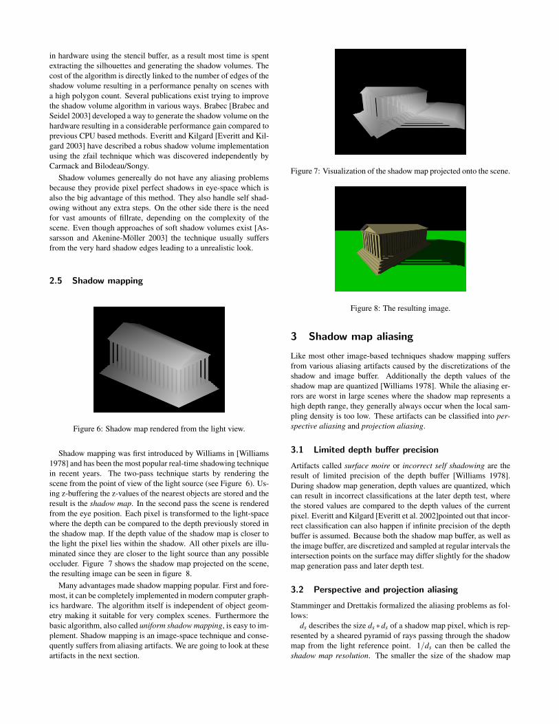
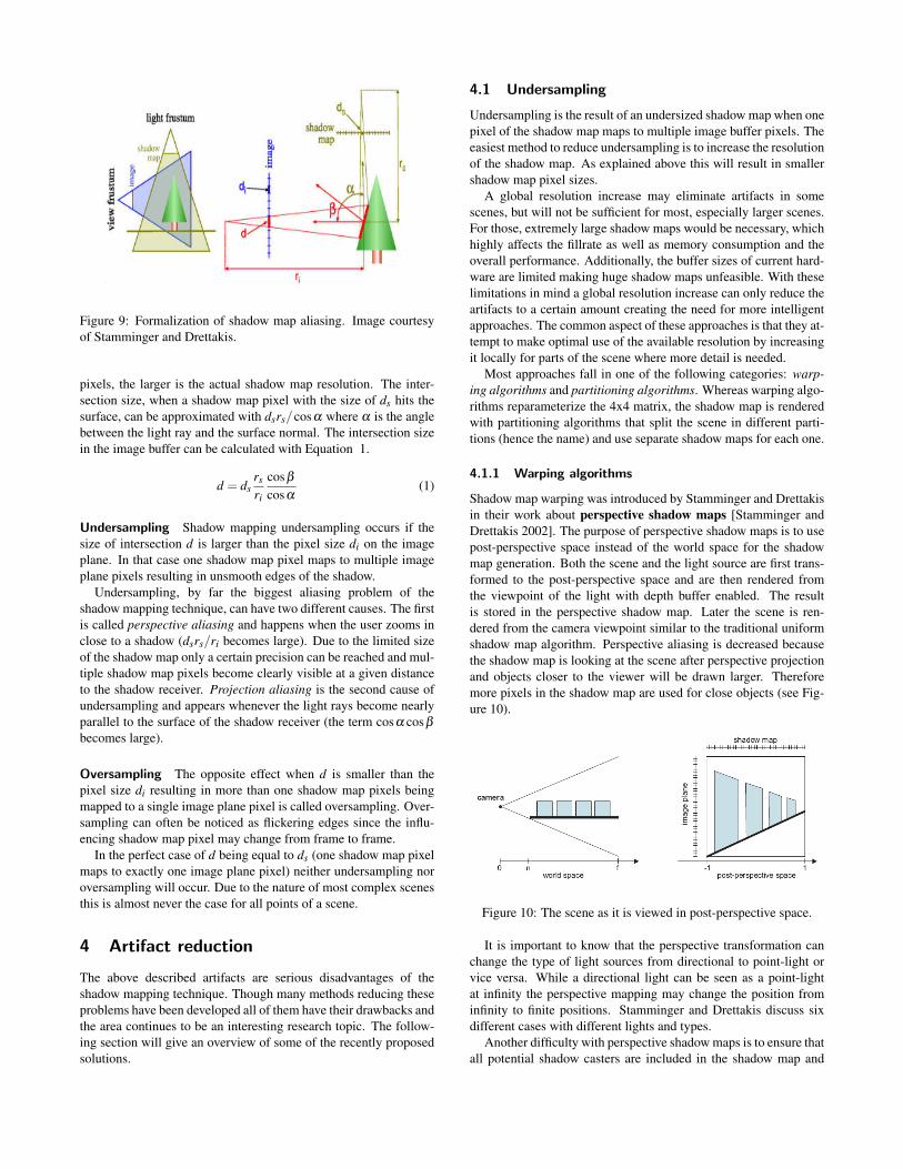
Shadow mapping was first introduced by Williams in [Williams1978] and has been the most popular real-time shadowing techniquein recent years. The two-pass technique starts by rendering thescene from the point of view of the light source (see Figure 6). Us-ing z-buffering the z-values of the nearest objects are stored and theresult is the shadow map. In the second pass the scene is renderedfrom the eye position. Each pixel is transformed to the light-spacewhere the depth can be compared to the depth previously stored inthe shadow map. If the depth value of the shadow map is closer tothe light the pixel lies within the shadow. All other pixels are illu-minated since they are closer to the light source than any possibleoccluder. Figure 7 shows the shadow map projected on the scene,the resulting image can be seen in figure 8.

Many advantages made shadow mapping popular. First and fore-most, it can be completely implemented in modern computer graph-ics hardware. The algorithm itself is independent of object geom-etry making it suitable for very complex scenes. Furthermore thebasic algorithm, also called uniform shadow mapping, is easy to im-plement. Shadow mapping is an image-space technique and conse-quently suffers from aliasing artifacts. We are going to look at theseartifacts in the next section.

Figure 7: Visualization of the shadow map projected onto the scene.

Figure 8: The resulting image.

3 Shadow map aliasing

Like most other image-based techniques shadow mapping suffersfrom various aliasing artifacts caused by the discretizations of theshadow and image buffer. Additionally the depth values of theshadow map are quantized [Williams 1978]. While the aliasing er-rors are worst in large scenes where the shadow map represents ahigh depth range, they generally always occur when the local sam-pling density is too low. These artifacts can be classified into per-spective aliasing and projection aliasing.

3.1 Limited depth buffer precision

Artifacts called surface moire or incorrect self shadowing are theresult of limited precision of the depth buffer [Williams 1978].During shadow map generation, depth values are quantized, whichcan result in incorrect classifications at the later depth test, wherethe stored values are compared to the depth values of the currentpixel. Everitt and Kilgard [Everitt et al. 2002]pointed out that incor-rect classification can also happen if infinite precision of the depthbuffer is assumed. Because both the shadow map buffer, as well asthe image buffer, are discretized and sampled at regular intervals theintersection points on the surface may differ slightly for the shadowmap generation pass and later depth test.

3.2 Perspective and projection aliasing

Stamminger and Drettakis formalized the aliasing problems as fol-lows:

ds describes the size ds ∗ds of a shadow map pixel, which is rep-resented by a sheared pyramid of rays passing through the shadowmap from the light reference point. 1/ds can then be called theshadow map resolution. The smaller the size of the shadow map

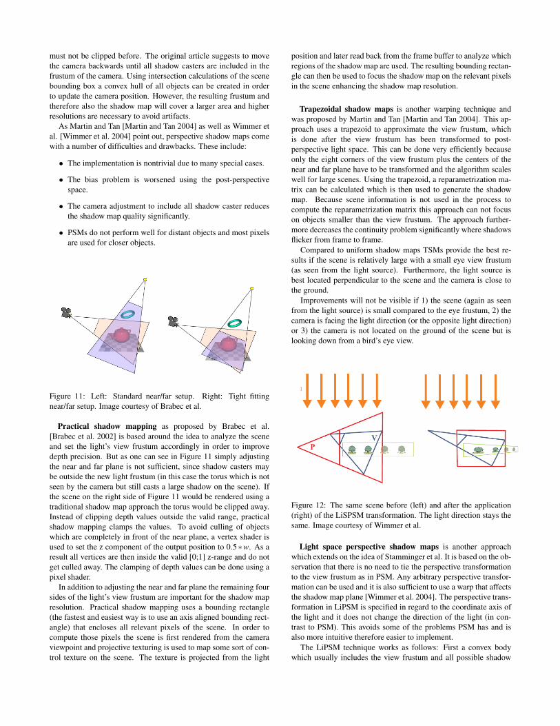
Figure 9: Formalization of shadow map aliasing. Image courtesyof Stamminger and Drettakis.

pixels, the larger is the actual shadow map resolution. The inter-section size, when a shadow map pixel with the size of ds hits thesurface, can be approximated with dsrs/cosα where α is the anglebetween the light ray and the surface normal. The intersection sizein the image buffer can be calculated with Equation 1.

d = dsrs

ri

cosβ

cosα(1)

Undersampling Shadow mapping undersampling occurs if thesize of intersection d is larger than the pixel size di on the imageplane. In that case one shadow map pixel maps to multiple imageplane pixels resulting in unsmooth edges of the shadow.

Undersampling, by far the biggest aliasing problem of theshadow mapping technique, can have two different causes. The firstis called perspective aliasing and happens when the user zooms inclose to a shadow (dsrs/ri becomes large). Due to the limited sizeof the shadow map only a certain precision can be reached and mul-tiple shadow map pixels become clearly visible at a given distanceto the shadow receiver. Projection aliasing is the second cause ofundersampling and appears whenever the light rays become nearlyparallel to the surface of the shadow receiver (the term cosα cosβ

becomes large).

Oversampling The opposite effect when d is smaller than thepixel size di resulting in more than one shadow map pixels beingmapped to a single image plane pixel is called oversampling. Over-sampling can often be noticed as flickering edges since the influ-encing shadow map pixel may change from frame to frame.

In the perfect case of d being equal to ds (one shadow map pixelmaps to exactly one image plane pixel) neither undersampling noroversampling will occur. Due to the nature of most complex scenesthis is almost never the case for all points of a scene.

4 Artifact reduction

The above described artifacts are serious disadvantages of theshadow mapping technique. Though many methods reducing theseproblems have been developed all of them have their drawbacks andthe area continues to be an interesting research topic. The follow-ing section will give an overview of some of the recently proposedsolutions.

4.1 Undersampling

Undersampling is the result of an undersized shadow map when onepixel of the shadow map maps to multiple image buffer pixels. Theeasiest method to reduce undersampling is to increase the resolutionof the shadow map. As explained above this will result in smallershadow map pixel sizes.

A global resolution increase may eliminate artifacts in somescenes, but will not be sufficient for most, especially larger scenes.For those, extremely large shadow maps would be necessary, whichhighly affects the fillrate as well as memory consumption and theoverall performance. Additionally, the buffer sizes of current hard-ware are limited making huge shadow maps unfeasible. With theselimitations in mind a global resolution increase can only reduce theartifacts to a certain amount creating the need for more intelligentapproaches. The common aspect of these approaches is that they at-tempt to make optimal use of the available resolution by increasingit locally for parts of the scene where more detail is needed.

Most approaches fall in one of the following categories: warp-ing algorithms and partitioning algorithms. Whereas warping algo-rithms reparameterize the 4x4 matrix, the shadow map is renderedwith partitioning algorithms that split the scene in different parti-tions (hence the name) and use separate shadow maps for each one.

4.1.1 Warping algorithms

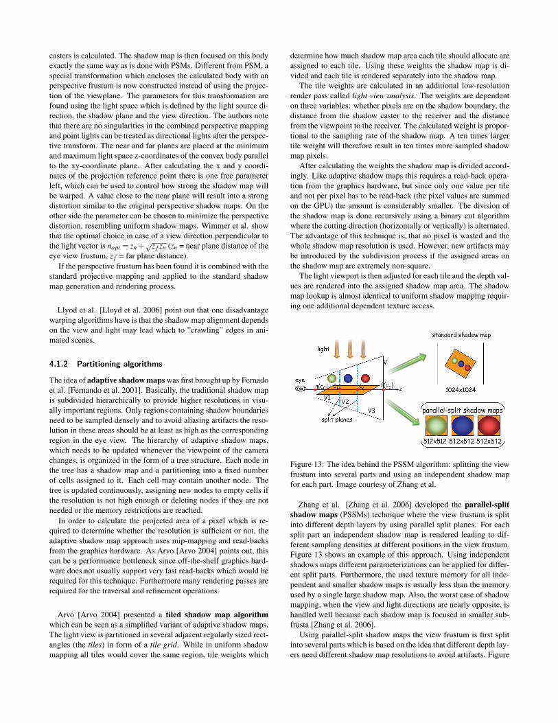
Shadow map warping was introduced by Stamminger and Drettakisin their work about perspective shadow maps [Stamminger andDrettakis 2002]. The purpose of perspective shadow maps is to usepost-perspective space instead of the world space for the shadowmap generation. Both the scene and the light source are first trans-formed to the post-perspective space and are then rendered fromthe viewpoint of the light with depth buffer enabled. The resultis stored in the perspective shadow map. Later the scene is ren-dered from the camera viewpoint similar to the traditional uniformshadow map algorithm. Perspective aliasing is decreased becausethe shadow map is looking at the scene after perspective projectionand objects closer to the viewer will be drawn larger. Thereforemore pixels in the shadow map are used for close objects (see Fig-ure 10).

Figure 10: The scene as it is viewed in post-perspective space.

It is important to know that the perspective transformation canchange the type of light sources from directional to point-light orvice versa. While a directional light can be seen as a point-lightat infinity the perspective mapping may change the position frominfinity to finite positions. Stamminger and Drettakis discuss sixdifferent cases with different lights and types.

Another difficulty with perspective shadow maps is to ensure thatall potential shadow casters are included in the shadow map and

must not be clipped before. The original article suggests to movethe camera backwards until all shadow casters are included in thefrustum of the camera. Using intersection calculations of the scenebounding box a convex hull of all objects can be created in orderto update the camera position. However, the resulting frustum andtherefore also the shadow map will cover a larger area and higherresolutions are necessary to avoid artifacts.

As Martin and Tan [Martin and Tan 2004] as well as Wimmer etal. [Wimmer et al. 2004] point out, perspective shadow maps comewith a number of difficulties and drawbacks. These include:

• The implementation is nontrivial due to many special cases.

• The bias problem is worsened using the post-perspectivespace.

• The camera adjustment to include all shadow caster reducesthe shadow map quality significantly.

• PSMs do not perform well for distant objects and most pixelsare used for closer objects.

Figure 11: Left: Standard near/far setup. Right: Tight fittingnear/far setup. Image courtesy of Brabec et al.

Practical shadow mapping as proposed by Brabec et al.[Brabec et al. 2002] is based around the idea to analyze the sceneand set the light’s view frustum accordingly in order to improvedepth precision. But as one can see in Figure 11 simply adjustingthe near and far plane is not sufficient, since shadow casters maybe outside the new light frustum (in this case the torus which is notseen by the camera but still casts a large shadow on the scene). Ifthe scene on the right side of Figure 11 would be rendered using atraditional shadow map approach the torus would be clipped away.Instead of clipping depth values outside the valid range, practicalshadow mapping clamps the values. To avoid culling of objectswhich are completely in front of the near plane, a vertex shader isused to set the z component of the output position to 0.5 ∗w. As aresult all vertices are then inside the valid [0;1] z-range and do notget culled away. The clamping of depth values can be done using apixel shader.

In addition to adjusting the near and far plane the remaining foursides of the light’s view frustum are important for the shadow mapresolution. Practical shadow mapping uses a bounding rectangle(the fastest and easiest way is to use an axis aligned bounding rect-angle) that encloses all relevant pixels of the scene. In order tocompute those pixels the scene is first rendered from the cameraviewpoint and projective texturing is used to map some sort of con-trol texture on the scene. The texture is projected from the light

position and later read back from the frame buffer to analyze whichregions of the shadow map are used. The resulting bounding rectan-gle can then be used to focus the shadow map on the relevant pixelsin the scene enhancing the shadow map resolution.

Trapezoidal shadow maps is another warping technique andwas proposed by Martin and Tan [Martin and Tan 2004]. This ap-proach uses a trapezoid to approximate the view frustum, whichis done after the view frustum has been transformed to post-perspective light space. This can be done very efficiently becauseonly the eight corners of the view frustum plus the centers of thenear and far plane have to be transformed and the algorithm scaleswell for large scenes. Using the trapezoid, a reparametrization ma-trix can be calculated which is then used to generate the shadowmap. Because scene information is not used in the process tocompute the reparametrization matrix this approach can not focuson objects smaller than the view frustum. The approach further-more decreases the continuity problem significantly where shadowsflicker from frame to frame.

Compared to uniform shadow maps TSMs provide the best re-sults if the scene is relatively large with a small eye view frustum(as seen from the light source). Furthermore, the light source isbest located perpendicular to the scene and the camera is close tothe ground.

Improvements will not be visible if 1) the scene (again as seenfrom the light source) is small compared to the eye frustum, 2) thecamera is facing the light direction (or the opposite light direction)or 3) the camera is not located on the ground of the scene but islooking down from a bird’s eye view.

Figure 12: The same scene before (left) and after the application(right) of the LiSPSM transformation. The light direction stays thesame. Image courtesy of Wimmer et al.

Light space perspective shadow maps is another approachwhich extends on the idea of Stamminger et al. It is based on the ob-servation that there is no need to tie the perspective transformationto the view frustum as in PSM. Any arbitrary perspective transfor-mation can be used and it is also sufficient to use a warp that affectsthe shadow map plane [Wimmer et al. 2004]. The perspective trans-formation in LiPSM is specified in regard to the coordinate axis ofthe light and it does not change the direction of the light (in con-trast to PSM). This avoids some of the problems PSM has and isalso more intuitive therefore easier to implement.

The LiPSM technique works as follows: First a convex bodywhich usually includes the view frustum and all possible shadow

casters is calculated. The shadow map is then focused on this bodyexactly the same way as is done with PSMs. Different from PSM, aspecial transformation which encloses the calculated body with anperspective frustum is now constructed instead of using the projec-tion of the viewplane. The parameters for this transformation arefound using the light space which is defined by the light source di-rection, the shadow plane and the view direction. The authors notethat there are no singularities in the combined perspective mappingand point lights can be treated as directional lights after the perspec-tive transform. The near and far planes are placed at the minimumand maximum light space z-coordinates of the convex body parallelto the xy-coordinate plane. After calculating the x and y coordi-nates of the projection reference point there is one free parameterleft, which can be used to control how strong the shadow map willbe warped. A value close to the near plane will result into a strongdistortion similar to the original perspective shadow maps. On theother side the parameter can be chosen to minimize the perspectivedistortion, resembling uniform shadow maps. Wimmer et al. showthat the optimal choice in case of a view direction perpendicular tothe light vector is nopt = zn +√z f zn (zn = near plane distance of theeye view frustum, z f = far plane distance).

If the perspective frustum has been found it is combined with thestandard projective mapping and applied to the standard shadowmap generation and rendering process.

Llyod et al. [Lloyd et al. 2006] point out that one disadvantagewarping algorithms have is that the shadow map alignment dependson the view and light may lead which to ”crawling” edges in ani-mated scenes.

4.1.2 Partitioning algorithms

The idea of adaptive shadow maps was first brought up by Fernadoet al. [Fernando et al. 2001]. Basically, the traditional shadow mapis subdivided hierarchically to provide higher resolutions in visu-ally important regions. Only regions containing shadow boundariesneed to be sampled densely and to avoid aliasing artifacts the reso-lution in these areas should be at least as high as the correspondingregion in the eye view. The hierarchy of adaptive shadow maps,which needs to be updated whenever the viewpoint of the camerachanges, is organized in the form of a tree structure. Each node inthe tree has a shadow map and a partitioning into a fixed numberof cells assigned to it. Each cell may contain another node. Thetree is updated continuously, assigning new nodes to empty cells ifthe resolution is not high enough or deleting nodes if they are notneeded or the memory restrictions are reached.

In order to calculate the projected area of a pixel which is re-quired to determine whether the resolution is sufficient or not, theadaptive shadow map approach uses mip-mapping and read-backsfrom the graphics hardware. As Arvo [Arvo 2004] points out, thiscan be a performance bottleneck since off-the-shelf graphics hard-ware does not usually support very fast read-backs which would berequired for this technique. Furthermore many rendering passes arerequired for the traversal and refinement operations.

Arvo [Arvo 2004] presented a tiled shadow map algorithmwhich can be seen as a simplified variant of adaptive shadow maps.The light view is partitioned in several adjacent regularly sized rect-angles (the tiles) in form of a tile grid. While in uniform shadowmapping all tiles would cover the same region, tile weights which

determine how much shadow map area each tile should allocate areassigned to each tile. Using these weights the shadow map is di-vided and each tile is rendered separately into the shadow map.

The tile weights are calculated in an additional low-resolutionrender pass called light view analysis. The weights are dependenton three variables: whether pixels are on the shadow boundary, thedistance from the shadow caster to the receiver and the distancefrom the viewpoint to the receiver. The calculated weight is propor-tional to the sampling rate of the shadow map. A ten times largertile weight will therefore result in ten times more sampled shadowmap pixels.

After calculating the weights the shadow map is divided accord-ingly. Like adaptive shadow maps this requires a read-back opera-tion from the graphics hardware, but since only one value per tileand not per pixel has to be read-back (the pixel values are summedon the GPU) the amount is considerably smaller. The division ofthe shadow map is done recursively using a binary cut algorithmwhere the cutting direction (horizontally or vertically) is alternated.The advantage of this technique is, that no pixel is wasted and thewhole shadow map resolution is used. However, new artifacts maybe introduced by the subdivision process if the assigned areas onthe shadow map are extremely non-square.

The light viewport is then adjusted for each tile and the depth val-ues are rendered into the assigned shadow map area. The shadowmap lookup is almost identical to uniform shadow mapping requir-ing one additional dependent texture access.

Figure 13: The idea behind the PSSM algorithm: splitting the viewfrustum into several parts and using an independent shadow mapfor each part. Image courtesy of Zhang et al.

Zhang et al. [Zhang et al. 2006] developed the parallel-splitshadow maps (PSSMs) technique where the view frustum is splitinto different depth layers by using parallel split planes. For eachsplit part an independent shadow map is rendered leading to dif-ferent sampling densities at different positions in the view frustum.Figure 13 shows an example of this approach. Using independentshadows maps different parameterizations can be applied for differ-ent split parts. Furthermore, the used texture memory for all inde-pendent and smaller shadow maps is usually less than the memoryused by a single large shadow map. Also, the worst case of shadowmapping, when the view and light directions are nearly opposite, ishandled well because each shadow map is focused in smaller sub-frusta [Zhang et al. 2006].

Using parallel-split shadow maps the view frustum is first splitinto several parts which is based on the idea that different depth lay-ers need different shadow map resolutions to avoid artifacts. Figure

Figure 14: The frustum is split along the z axis in parts at splitpositions Ci. Image courtesy of Zhang et al.

14 shows an example of a view frustum which is split into parts atcertain positions Ci. The PSSM approach describes three differentschemes to select the split positions: uniform split scheme, loga-rithmic split scheme and practical split scheme which combines thefirst two (see Figure 15).

Figure 15: The three different split schemes. Image courtesy ofZhang et al.

As we have shown above, the optimal distribution of perspectivealiasing errors make d p/ds constant and the logarithmic functionis used to approximate this distribution. The more split parts thatare used in order to discretize the logarithmic function, the closerthe distribution will to the ideal. The problem with the logarithmicsplit scheme is, that the split parts close to the viewer are too smalland only a few objects will be included. Zhang et al. describe that”this is due to the theoretically optimal parameterization assumesthat the shadow map accurately covers the view frustum and noany resolution is wasted on invisible parts of the scene.” In practicethis leads to over-sampling in parts near to the viewer and under-sampling in parts further from the viewer.

The uniform split scheme simply splits the frustum uniformlyalong the z axis. Similar to uniform shadow mapping this schemeresults in under-sampling at points closer to the viewer because thedistribution of perspective aliasing errors is the same. Furthermoreover-sampling is introduced in points further away.

Both, logarithmic and uniform split schemes, do not produceappropriate sampling densities for the whole scene. The practi-cal split scheme is designed to combine the advantages of bothwhile reducing their draw backs and aliasing origins. The calcu-lated split positions Cuni f orm

i and Clogarithmici are simply combined

by Ci = (Cuni f ormi +Clogarithmic

i )/2. See equation 2 for the completecomputation.

Ci =n( f /n)i/m+n+( f −n)i/m

2+δbias (2)

notation descriptionCi depth of the i-th split planen near planef far planem number of splitsi current split

Besides splitting the view frustum as explained above the lightfrustum W is also split into smaller parts Wi. Each of the light frus-tum parts covers one view frustum part Viand the bounding boxesof these view frustum split parts are used to focus the light frus-tum parts on the relevant areas. Afterwards each split part Vi isrendered to an independent shadow map Ti using the light spaceWi. Shadow map sizes of 512x512 are usually sufficient and othershadow mapping techniques such as the before described warpingapproaches can be integrated into PSSMs. Generally three splitsalready produce good results and use less memory than one uni-form 1024x1024 map. Since additional splits result in additionalrender passes the performance decreases with an increasing num-ber of splits. Zhang et al. eliminated this problem by integratingthe shadow map selection into the pixel shader which is possible aslong as the number of splits does not excess the number of availabletextures.

Figure 16: Six shadow map algorithms compared. Images courtesyof Zhang et al.

Experiments have shown that parallel split shadow maps workextremely well for very large environments. The example in Figure

16 is a outdoor environment rendered in the view frustum with near= 1m and far = 1000m. There are about 55 complex objects ran-domly located in the 2.56km2 environment. The authors state thatrendering performance of the 1.3 million polygons was almost thesame for all methods used.

4.1.3 Other approaches

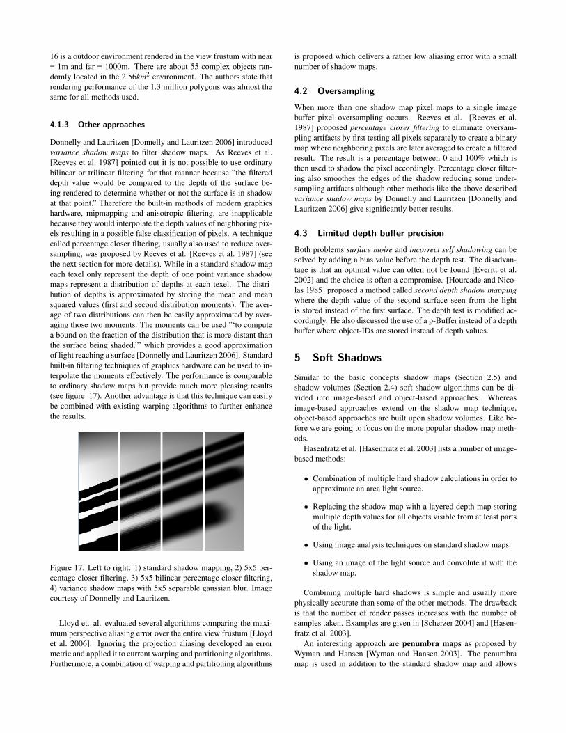
Donnelly and Lauritzen [Donnelly and Lauritzen 2006] introducedvariance shadow maps to filter shadow maps. As Reeves et al.[Reeves et al. 1987] pointed out it is not possible to use ordinarybilinear or trilinear filtering for that manner because ”the filtereddepth value would be compared to the depth of the surface be-ing rendered to determine whether or not the surface is in shadowat that point.” Therefore the built-in methods of modern graphicshardware, mipmapping and anisotropic filtering, are inapplicablebecause they would interpolate the depth values of neighboring pix-els resulting in a possible false classification of pixels. A techniquecalled percentage closer filtering, usually also used to reduce over-sampling, was proposed by Reeves et al. [Reeves et al. 1987] (seethe next section for more details). While in a standard shadow mapeach texel only represent the depth of one point variance shadowmaps represent a distribution of depths at each texel. The distri-bution of depths is approximated by storing the mean and meansquared values (first and second distribution moments). The aver-age of two distributions can then be easily approximated by aver-aging those two moments. The moments can be used ”‘to computea bound on the fraction of the distribution that is more distant thanthe surface being shaded.”’ which provides a good approximationof light reaching a surface [Donnelly and Lauritzen 2006]. Standardbuilt-in filtering techniques of graphics hardware can be used to in-terpolate the moments effectively. The performance is comparableto ordinary shadow maps but provide much more pleasing results(see figure 17). Another advantage is that this technique can easilybe combined with existing warping algorithms to further enhancethe results.

Figure 17: Left to right: 1) standard shadow mapping, 2) 5x5 per-centage closer filtering, 3) 5x5 bilinear percentage closer filtering,4) variance shadow maps with 5x5 separable gaussian blur. Imagecourtesy of Donnelly and Lauritzen.

Lloyd et. al. evaluated several algorithms comparing the maxi-mum perspective aliasing error over the entire view frustum [Lloydet al. 2006]. Ignoring the projection aliasing developed an errormetric and applied it to current warping and partitioning algorithms.Furthermore, a combination of warping and partitioning algorithms

is proposed which delivers a rather low aliasing error with a smallnumber of shadow maps.

4.2 Oversampling

When more than one shadow map pixel maps to a single imagebuffer pixel oversampling occurs. Reeves et al. [Reeves et al.1987] proposed percentage closer filtering to eliminate oversam-pling artifacts by first testing all pixels separately to create a binarymap where neighboring pixels are later averaged to create a filteredresult. The result is a percentage between 0 and 100% which isthen used to shadow the pixel accordingly. Percentage closer filter-ing also smoothes the edges of the shadow reducing some under-sampling artifacts although other methods like the above describedvariance shadow maps by Donnelly and Lauritzen [Donnelly andLauritzen 2006] give significantly better results.

4.3 Limited depth buffer precision

Both problems surface moire and incorrect self shadowing can besolved by adding a bias value before the depth test. The disadvan-tage is that an optimal value can often not be found [Everitt et al.2002] and the choice is often a compromise. [Hourcade and Nico-las 1985] proposed a method called second depth shadow mappingwhere the depth value of the second surface seen from the lightis stored instead of the first surface. The depth test is modified ac-cordingly. He also discussed the use of a p-Buffer instead of a depthbuffer where object-IDs are stored instead of depth values.

5 Soft Shadows

Similar to the basic concepts shadow maps (Section 2.5) andshadow volumes (Section 2.4) soft shadow algorithms can be di-vided into image-based and object-based approaches. Whereasimage-based approaches extend on the shadow map technique,object-based approaches are built upon shadow volumes. Like be-fore we are going to focus on the more popular shadow map meth-ods.

Hasenfratz et al. [Hasenfratz et al. 2003] lists a number of image-based methods:

• Combination of multiple hard shadow calculations in order toapproximate an area light source.

• Replacing the shadow map with a layered depth map storingmultiple depth values for all objects visible from at least partsof the light.

• Using image analysis techniques on standard shadow maps.

• Using an image of the light source and convolute it with theshadow map.

Combining multiple hard shadows is simple and usually morephysically accurate than some of the other methods. The drawbackis that the number of render passes increases with the number ofsamples taken. Examples are given in [Scherzer 2004] and [Hasen-fratz et al. 2003].

An interesting approach are penumbra maps as proposed byWyman and Hansen [Wyman and Hansen 2003]. The penumbramap is used in addition to the standard shadow map and allows

polygonal objects to cast approximate soft shadows on themselvesand other objects. In a three pass process a standard shadow map iscreated before the penumbra map is calculated in the second pass.The penumbras themselves are constructed using cones and sheets.The first pass then uses the intensity information from the penumbramap in combination with the shadow map’s depth information torender the scene.

While penumbra maps can be quite easily integrated in exist-ing shadow map algorithms, their performance suffers especially inscenes with a high polygon count. A significant amount of time isspent calculating the penumbra.

Figure 18: Left to right: a) standard shadow map, b) smoothiebuffer (depth values), c) smoothie buffer (alpha values), d) finaleimage. Image courtesy of Chan and Durant.

Another variation of the shadow map approach are the so calledsmoothies. The algorithm first renders an ordinary shadow mapand then extracts the silhouettes of the shadow occluders. Similarto penumbra maps the silhouettes are then extended by geometricprimitives (the smoothies) which are later rendered into a smoothiebuffer. In addition to the smoothie depth an alpha value which de-pends on the ratio of distances distances between the light source,blockers and receiver is stored. Finally the image is rendered byusing the shadow map and smoothie buffer to determine whetherand how a point is shadowed. See Figure 18 for an overview of theprocess.

Both, smoothies and penumbra maps only compute the outerpenumbra, which makes scenes a lot darker than anticipated be-cause shadow occluders will always project an umbra even if thelight source is very large. One approach that handles inner andouter-penumbras is the soft shadow map technique [Atty et al.2006].

The algorithm starts by dividing occluders and receivers, one ob-ject can not be occluder and receiver at the same time and the softshadows are only generated from the occluders onto the receivers.Instead of one depth, buffer two buffers, one for the occluders andone for the receivers, are computed. The occluder depth buffers isconverted into a set of rectangles or so called micro-patches. Thesize of these rectangles depends on the distance from light sourceto the pixel in the occluder buffer. The further away a pixel is thelarger the resulting rectangle.

The depth values of the receivers are stored in the receiver buffer.In order to compute the soft shadow map for each light source,the soft shadow for every occluder micro-patch is calculated andsummed. This calculation takes the relative distance between theoccluders, the receiver and the light source into account. Given thefact that the micro-patches are parallel to the light source this com-putation can be done quite fast.

While the algorithm is fast and provides good results the largestlimitation is the fact that self-shadowing is not supported. Also,the technique can not be easily integrated into existing hard shadow

map methods.

This was only a short overview of some of the existing softshadow mapping techniques. For more take a look at the surveysof Hasenfratz et al. [Hasenfratz et al. 2003] and Scherzer [Scherzer2004].

6 Conclusion

While shadow mapping became very popular in recent years be-cause of the simplicity of the basic algorithm, we have seen thatvarious aliasing artifacts such as perspective and projection alias-ing make new approaches and extensions of the original uniformshadow mapping technique necessary.

In order to understand the problems involved, the basic con-cepts of hard and soft shadows as well as the two most populartechniques, shadow volumes and shadow mapping were explained.Later we gave a detailed look into the possible aliasing artifactsand described some of the most important methods to reduce them.These methods were classified in regard to what aliasing artifactthey are supposed to eliminate. Most research goes into the reduc-tion of undersampling artifacts and all ideas are based on the idea toprovide a higher shadow map resolution were needed and a lowersampling density for distant regions. Most proposed methods canbe divided into warping and partitioning algorithms. Whereas theformer modify the perspective transform in order to reach the goal,the latter divide the shadow map or the view frustum in smaller partsfor specific regions of the scene. These parts can be handled indi-vidually and their size varies depending on the requested shadowmap size.

At the end a short overview of existing soft shadow techniqueswas given, introducing even more challenges to the already com-plex area of real-time shadows. After studying this paper the readershould be able to understand the basic concepts and problems ofreal-time shadows. Choosing a shadowing technique is not a sim-ple task since due to the nature of the problem there is no singleideal or optimal solution. Therefore, I hope that this paper can helpa reader get started in this interesting field of computer graphics.

References

ARVO, J. 2004. Tiled shadow maps. In CGI ’04: Proceedings ofthe Computer Graphics International (CGI’04), IEEE ComputerSociety, Washington, DC, USA, 240–247.

ASSARSSON, U., AND AKENINE-MOLLER, T. 2003. A geometry-based soft shadow volume algorithm using graphics hardware. InSIGGRAPH ’03: ACM SIGGRAPH 2003 Papers, ACM Press,New York, NY, USA, 511–520.

ATTY, L., HOLZSCHUCH, N., LAPIERRE, M., HASENFRATZ, J.-M., HANSEN, C., AND SILLION, F. 2006. Soft shadow maps:Efficient sampling of light source visibility. Computer GraphicsForum 25, 4 (dec). (to appear).

BRABEC, S., AND SEIDEL, H.-P. 2003. Shadow volumes on pro-grammable graphics hardware. In Eurographics 2003.

BRABEC, S., ANNEN, T., AND SEIDEL, H.-P. 2002. Practicalshadow mapping. J. Graph. Tools 7, 4, 9–18.

CROW, F. C. 1977. Shadow algorithms for computer graphics.In SIGGRAPH ’77: Proceedings of the 4th annual conferenceon Computer graphics and interactive techniques, ACM Press,New York, NY, USA, 242–248.

DONNELLY, W., AND LAURITZEN, A. 2006. Variance shadowmaps. In SI3D ’06: Proceedings of the 2006 symposium on In-teractive 3D graphics and games, ACM Press, New York, NY,USA, 161–165.

EVERITT, C., AND KILGARD, M. J., 2003. Practical and robuststenciled shadow volumes for hardware-accelerated rendering.

EVERITT, C., REGE, A., AND CEBENOYAN, C., 2002. Hardwareshadow mapping.

FERNANDO, R., FERNANDEZ, S., BALA, K., AND GREENBERG,D. P. 2001. Adaptive shadow maps. In SIGGRAPH ’01: Pro-ceedings of the 28th annual conference on Computer graphicsand interactive techniques, ACM Press, New York, NY, USA,387–390.

HASENFRATZ, J.-M., LAPIERRE, M., HOLZSCHUCH, N., AND

SILLION, F. 2003. A survey of real-time soft shadows algo-rithms. Computer Graphics Forum 22, 4 (dec), 753–774.

HOURCADE, J. C., AND NICOLAS, A. 1985. Algorithms for an-tialiased cast shadows. Computers and Graphics 9, 3, 259–265.

LLOYD, B., TUFT, D., YOON, S., AND MANOCHA, D. 2006.Warping and partitioning for low error shadow maps. In Pro-ceedings of the Eurographics Symposium on Rendering 2006,Eurographics Association, 215–226.

MARTIN, T., AND TAN, T.-S. 2004. Anti-aliasing and continuitywith trapezoidal shadow maps. In Rendering Techniques, 153–160.

REEVES, W. T., SALESIN, D. H., AND COOK, R. L. 1987. Ren-dering antialiased shadows with depth maps. SIGGRAPH Com-put. Graph. 21, 4, 283–291.

SCHERZER, D. 2004. Real-time soft shadows. In Europgrahics.

STAMMINGER, M., AND DRETTAKIS, G. 2002. Perspectiveshadow maps.

WILLIAMS, L. 1978. Casting curved shadows on curved surfaces.In SIGGRAPH ’78: Proceedings of the 5th annual conferenceon Computer graphics and interactive techniques, ACM Press,New York, NY, USA, 270–274.

WIMMER, M., SCHERZER, D., AND PURGATHOFER, W. 2004.Light space perspective shadow maps. In Rendering Techniques2004 (Proceedings of the Eurographics Symposium on Ren-dering 2004), Eurographics Association, A. Keller and H. W.Jensen, Eds., Eurographics, 143–151.

WOO, A., POULIN, P., AND FOURNIER, A. 1990. A survey ofshadow algorithms. IEEE Comput. Graph. Appl. 10, 6, 13–32.

WYMAN, C., AND HANSEN, C. 2003. Penumbra maps: approx-imate soft shadows in real-time. In EGRW ’03: Proceedingsof the 14th Eurographics workshop on Rendering, EurographicsAssociation, Aire-la-Ville, Switzerland, Switzerland, 202–207.

ZHANG, F., SUN, H., XU, L., AND LUN, L. K. 2006. Parallel-split shadow maps for large-scale virtual environments. In VR-CIA ’06: Proceedings of the 2006 ACM international conferenceon Virtual reality continuum and its applications, ACM Press,New York, NY, USA, 311–318.