Real-time simulation of three phase Induction motor using

Raspberry Pi

Thesis submitted in partial fulfillment of the requirements for the degree of

Master of Technology

in

Electrical Engineering (Specialization: Power electronics and Drives)

by

Surapu Jagan

Department of Electrical Engineering National Institute of Technology Rourkela

Odisha, 769008, India May 2015

Dissertation submitted

In May 2015

To the department of

Electrical Engineering Of

National Institute of Technology Rourkela

In partial fulfillment of the requirements for the degree of

Master of Technology

By

Surapu Jagan (Roll: 213EE4323 )

Under the supervision of

Prof. S. Gopala Krishna

Real-time simulation of three phase Induction motor using

Raspberry Pi

Department of Electrical Engineering

National Institute of Technology Rourkela, Odisha-769008

Department of Electrical Engineering National Institute of Technology Rourkela Rourkela-769008, Odisha, India.

Certificate

This is to certify that the work in the thesis entitled Real-time simulation of three phase

induction motor using Raspberry Pi by S ur a p u J a g a n is a record of an original research

work carried out by him under my supervision and guidance in partial fulfillment of the

requirements for the award of the degree of Master of Technology with the specialization

of Power electronics & Drives in the department of Electrical Engineering, National

Institute of Technology Rourkela. Neither this thesis nor any part of it has been submitted

for any degree or academic award elsewhere.

Place: NIT Rourkela Prof. S. Gopala Krishna Date: May 2015 Professor, EE Department

NIT Rourkela, Odisha

i

Acknowledgment

It is a genuine pleasure to express my deep sense of thanks and gratitude to my

mentor and guide Dr. S. Gopala Krishna, Assistant professor, Department of electrical

engineering, NIT Rourkela, Odisha. His desiccation and keen interest above all

overwhelming attitude to help his students had been responsible for completing my work. His

timely advice, meticulous scrutiny advice and scientific approach have helped me a little to

accomplish this task.

I owe a deep sense of gratitude to Dr. A.K.Panda, Head of the department,

department of electrical engineering, NIT Rourkela, Odisha for providing me all the required

facilities. I would like to thank all the other faculties of electrical department for their

guidance. I thank profusely all the Staff of NIT Rourkela for their help and cooperation

throughout my study period.

I am extremely thankful to my friends for giving continuous support and helpful

company. My wholehearted gratitude to my parents and brother for their encouragement and

support.

Surapu Jagan

Roll. No: 213EE4323

ii

Abstract

These days’ simulators are playing a crucial role in day to day life. In order to reduce

the cost and effort, people are preferring simulation rather than going for hardware. But this

normal simulations can’t give a good idea of the system behavior. For much better

understanding of the system real time simulation is the only option. This comes under a

special case of normal digital simulations. In this thesis topics like, what is real time

simulation means and what are its requirements are explained in detail. Some of the daily life

real-time simulation applications have also been illustrated in a detailed manner. By the

advancements in software technologies many simulation tools are available in the market for

real time simulation such as RT-lab, eFPGAsim, MATLAB/SIMULINK. These real time

simulators bridges the gap between theoretical knowledge and practical knowledge. Thus

these are very helpful for students and researchers to get practical experience with greater

flexibility, without going for the costly and bulky physical equipment.

The main objective of this project is to simulate a low cost real time simulator. In this

project real time simulation has been done using Raspberry Pi kit as the hardware simulator

and Python Language as Real-time simulation software. In this thesis capability of Raspberry

pi and its interfacing with outer world has been discussed in detail. The reason for selecting

python and its advantages are also explained in detail here.

In this thesis, topics like how the model of the induction motor can be represented in

differential equations is also discussed in detail. There are also discussions about the different

numerical methods that can be used to solve these differential equations and the suitability of

these methods to a particular application.

iii

Contents

1. Introduction ………………………………………………….....................................2

1.1 Motivation …………………………………………………………….3

1.2 Literature Review ………………………………………………………3

1.3 Objective and scope …………………………………………………….3

2. Real-time simulation ………………………………………………………………...5

2.1 Introduction to real-time simulation ……………………………………...6

2.2Types of real time simulation ……………………………………………9

2.2.1 Rapid control prototyping

2.2.2 Hardware-in-the-Loop simulation

2.2.3 Software-in-the-Loop simulation

2.3 Applications of Real-time simulation …………………………………11

3. Requirements of Real-time simulation ………………………………………………16

3.1 Introduction to Raspberry Pi .……………………………………………18

3.1.1 Interfacing ports

3.1.2 Applications of Raspberry Pi

3.2 Introduction to Python …………………………………………………..20

3.2.1 Advantages and capabilities of Python

3.3 Numerical integration methods ………………………………………....22

3.4 Modelling of three phase induction motor ………………………………25

4. Real-time simulation in Raspberry Pi ……………………………………………….30

4.1 simulation results ………………………………………………………..33

5. Real time simulation in MATLAB …………………………………………………..36

5.1 Simulation results ………………………………………………………..39

6. Conclusion and Bibliography ………………………………………………………..43

Appendix-A: Simulation of induction motor using SIMULINK …………………....46

iv

List of figures Fig.no Figure name Pg.no

Fig. 1.1 Comparison between real time and non-real time simulations 7

Fig. 2.1 Rapid control prototyping 10

Fig. 2.2 Hardware in loop simulation 10

Fig. 2.3 Software in loop simulation [SIL] 11

Fig. 2.4 Multi-level VSC based STATCOM 12

Fig. 2.5 Real-time simulation of Renewable energy sources 12

Fig. 2.6 Hybrid electric vehicle model 13

Fig. 2.7 Electric motor drive model 14

Fig. 3.1 The Raspberry Pi hardware kit 19

Fig. 3.2 Graphical representation of a function (ݔ) 23

Fig. 4.1 The electromagnetic torque vs rotor speed of 3-phase induction motor in Raspberry Pi simulation

33

Fig. 4.2 The stator current of 3-phase induction motor in Raspberry Pi simulation 33

Fig. 4.3 The rotor current of 3-phase induction motor in Raspberry Pi simulation 34

Fig. 4.4 The electromagnetic torque of 3-phase induction motor in Raspberry Pi simulation

34

Fig. 4.5 The rotor speed of 3-phase induction motor in Raspberry Pi simulation 34

Fig. 4.6 The D-axis stator current of 3-phase induction motor in Raspberry Pi simulation

35

Fig. 4.7 The Q-axis stator current of 3-phase induction motor in Raspberry Pi simulation

35

Fig. 4.8 The D-axis rotor current of 3-phase induction motor in Raspberry Pi simulation

35

Fig. 4.9 The Q-axis stator current of 3-phase induction motor in Raspberry Pi simulation

35

Fig. 5.1 The D-axis stator current of 3-phase induction motor in MATLAB simulation

39

Fig. 5.2 The Q-axis stator current of 3-phase induction motor in MATLAB simulation

40

Fig. 5.3 Comparison between D-axis and Q-axis stator currents of 3-phase induction motor in MATLAB simulation

40

Fig. 5.4 The D-axis rotor current of 3-phase induction motor in MATLAB simulation

40

v

Fig. 5.5 The Q-axis rotor current of 3-phase induction motor in MATLAB simulation

41

Fig. 5.6 The Rotor speed of 3-phase induction motor in MATLAB simulation 41

Fig. 5.7 The electromagnetic torque vs rotor speed of 3-phase induction motor in MATLAB simulation

42

Fig. I The SIMULINK block diagram of 3-phase induction motor 46

Fig. II The inside architecture of the SIMULINK block of 3-phase induction motor 46

Fig. III The stator current of 3-phase induction motor in SIMULINK simulation 47

Fig. IV The stator current of 3-phase induction motor in SIMULINK simulation 47

Fig. V The electromagnetic torque of 3-phase induction motor in SIMULINK simulation

48

Fig. VI The rotor speed of 3-phase induction motor in SIMULINK simulation 48

Fig. VII The electromagnetic torque vs rotor speed of 3-phase induction motor in SIMULINK simulation

49

Chapter 1

Introduction

2

Introduction

Nowadays Simulators are extensively used in the planning and designing of electrical

systems for several years. Starting from the layout of transmission lines in large scale power

systems to the optimization of motor drives in transportation, simulators has been playing a

crucial role for the last thirty years. The evolution of different computing technologies leads to

the evolution of many simulation tools, thereby enabling the user to work in different simulation

environments. Because of the steady decrease in cost of computer technologies and an increase

in their performance features, the solving capability of simulators has been improved. Almost

any complex problems can be solved in very less time and with good accuracy. Thus the user is

getting the benefit of saving time and better understanding of their work.

There are two different types of simulation environment. One is a Real-

timesimulation and other is a Non-real time simulation or offline simulation. Most of the

applications use offline simulation because of lesser cost and quick performance. But when we

require exact model performance characteristics of the original model, we have to go for Real-

time simulation. Real-time simulation can be defined as simulation of a virtual model of a

physical system that can perform the given task at the same rate as an actual Real time clock.

That means the virtual computer model runs at the same rate as the actual physical system. For

example Simulation of the system’s response to 1 second must be completed in exactly1 second

These days, people are more concerned about the comfort ability and ease of the

simulator. There are certain simulators in the market, which can enable us to vary the simulation

step size and many other variables of the simulation. In these simulations, we don’t need to

worry about whether the numerical integration is going to meet our accuracy requirement or not.

The simulation algorithm does that work. Whereas in Real–time simulation, we can’t get all this

comfort. In order to understand ourselves how our simulation works in Real, we have to satisfy

some of the modern features of our simulation which can save time.

3

Now a days real-time simulators are being used immensely in engineering and

construction fields. In applications like Statistical power grid protection tests and Motor drive

controller designing methods these simulators are playing a crucial role. These are not only used

in these applications but also in applications like space robot integration and Air vehicle design

and test simulation.

1.1Motivation The real-time simulators that are being used in daily life are of highly expensive and

complex to operate. It requires qualified technical staff to operate this system. A low cost real-

time simulator enables the user to work on some simple systems. It also provides easiness to user

while operating. For example, if an engineer want to test a three phase induction motor, he don’t

need to go to expensive real-time simulators instead he can opt a low cost real-time simulator for

his application

1.2 Objective

The main objective of this project is

To design and simulate real time model of Induction motor on low cost

Raspberry Pi

To explore the capabilities of Raspberry pi hardware and test whether

real-time simulation is possible on it or not

1.3 Literature review With the purpose of doing real-time simulation on any platform, one must know deeply

about what is the real-time simulation, what its requirements are, where it can be used and why it

is used. These three things are explained elaborately with examples in [1]. The main objective of

this project is to do real-time simulation on Raspberry Pi so in depth details about its architecture

and capabilities should be known. These are well explained in [2]. This paper also explains how

one can make use of Raspberry Pi for the real-time simulation elaborately. In order to do real

4

time simulation of a system, modelling a mathematical model of the system is important. In this

paper a dynamic model of 3-phase induction motor is modelled using differential equations. This

is well explained in the paper [3].

After that a software is required to write a program for designing of a real-time model

that has to be expressed in the form of differential equations. In this project python is used for

this purpose. So knowing about Python and its programming is necessary. This software can be

downloaded from the website [6]. The python programming is well explained with examples in

the website [6, 7] and work out some examples. For the purpose of real time simulation, the

Knowledge of various numerical integration methods with detailed comparison is required. The

various advantages and disadvantages of different methods and which method is suitable for a

particular purpose can also learnt in the text book [4].

In order to do real-time simulation using MATLAB, the MATLAB programming is

illustrated with examples in [7,8and 13]. Here there are some examples and discussions relating

to our project. The real-time simulation using MATLAB is explained elaborately in [9]. The

questions like how to update the data keeping the previous data on the plot and the associated

problems and possible solutions are explained in detailed manner in [9, 10]. There are discussion

about similar projects in the website [11, 12].

5

Chapter 2

Real-time simulation

6

Real-Time Simulation 2.1 Introduction

Real-time simulation is defined as the numerical solution of the mathematical model of a

given physical system where the simulation time is equal to real time. The real-time simulation

of a system is very similar to the actual physical system in the point of variation of simulated

quantities with real-world clock time. This is the major difference between the offline simulation

and the real-time simulation. Real-time simulation simply replicates the characteristics of a

physical system as it is also running with respect to real time. In offlinesimulation the numerical

integration time step is a number in the software, whereas in real-time simulation, the hardware

timer provides this time step.

For a given time-step we have to solve mathematical equations and functions within that

time step that means each variable involved in simulation or the state of the system should be

solved [by numerical integration] iteratively as a function of variables used in simulation and the

system states at the end of the preceding time step.In the discrete time simulation, the time

(actual clock time) taken to solve all the equations that are representing our physical system at

the given time-step can be more or less than the provided time-step.

For better understanding of the Real-time simulation, observe the figure 1.1 which shows

the difference between offline simulation and real-time simulation. In the first case, we can

observe that the computation time for each iteration is shorter than the fixed time-step (of real

time clock). This type of simulation is called accelerated simulation. Whereas in the second case,

the computation time is longer than the fixed time-step (of real time clock). These two types of

simulations can be called as offline simulation. In these two cases, we can’t predict the moment

at which the result will be available. Thus the main objective in performing an offline simulation

is getting the results as early as possible depending on co. The calculation speed in offline

simulation depends mainly on the Processor Speed and complexity of system’s mathematical

model.

7

In contrast to offline simulation, during real time simulation, the accuracy of

computations involved in system simulation will be depending on exact dynamic representation

of the system in mathematical model and the time period assigned to generate results. We can

see that the results are available exactly at the end of each simulation time step. Thus we can

predict occurrence of the result. Figure 1.1 depicts the difference between the offline and real-

time simulations.

Fig1.1: Comparison between real time and non-real time simulations

For a valid real-time simulation, the simulator used should generate the internal variables

and outputs of the simulation within the same period that its actual real world system do. The

time taken to calculate the solution at the given time step should be less than the real-world clock

time step. If the simulator computes the dynamic model equations before the allocated time step,

then it will wait until the next real-time clock time-step starts. If the simulator can’t compute the

equations within allocated fixed time-step, then the system is out of synchronism, and the

simulation is no longer real-time simulation. This is called as “overrun”.

8

The simulator should execute a series of tasks for each time step iteratively:

Reading inputs and generating outputs

Solve real-time model equations in differential form by using suitable numerical

integration method

Exchanging these results with the previous results

Wait for the next time-step to start

Mainly there are two applications, where the real-time simulation is mandatory. First one

is; the developer uses the real-time simulator to validate their control algorithm against its

working conditions with the plant. In particular, when there is analog power electronics involved.

The simulation of these components is very difficult, so real hardware is needed. As the virtual

model of the plant is being used, the controller need not to be in its fully designed form. The

second application is, the developer may want to check his required functional behavior of the

finished the product, such as power usage or heat or fault conditions. That means the developer

want to check whether it is working under predicted conditions or not.

The main challenge that an engineer will face while doing real time simulation is the

selection of the real-time simulator to meet his requirements. The simulator size, cost and other

characteristics will be depending on two main factors. They are:

The highest transient frequency to be simulated, which also decides the minimum

integration time-step to be used

The System size and complexity of simulation

The number of Input/output channels used for interfacing our simulator with the physical

controller is also an important factor to be considered.

For example take a situation where we have to trigger a thyrister at an angle 90 degrees

with respect to the AC voltage source positive zero crossing. When the thyrister triggers, the

current begins to flow in it. If we compare the load current waveform obtained in non-real time

simulation and the waveform obtained in real-time simulation, we can observe certain error in

the non-real time case. The reason is the 90 electrical degrees event was not occurred in

synchronous with the simulator fixed time-step. Hence, the thyrister gate signal is taken into

consideration only at the beginning of the next time-step. This phenomenon is called as “jitter”.

9

Whenever jitter comes into picture there will be considerable uncharacteristic harmonics

introduced into the waveforms. Thus resulting in in valid simulation results.

High frequency power electronic converters ranging from 10-50 kHz may require very

small time-steps of less than 10 microseconds. Higher resonant frequency circuits will be

requiring a time–step of below 20 micro seconds. Example: Low-voltage distribution circuits,

electric rail power feeding systems etc.

The real time model can be interacted in 3 ways. They are

(a) interaction with a system user

(b) interaction with physical equipment

(c) interaction with both at the same time

In first two cases we can give inputs to the real- time model and get outputs from it, in

same way we do with the physical plant. But one advantage of the real-time model is that we can

run the model online. That means it can be modified during the simulation, which can’t be

achieved with a real physical plant. Not only that we can also read and update any parameter of

the model online. For instance, take a simulation of a small power plant, while running the

simulation we can change the inertia of the turbine to know its effect on the stability of the

system. This we can’t do with the physical power plant. By using a real-time model, almost

every model quantity can be accessed during execution. For example take a wind turbine. The

torque we inject on the generator from a gearbox can be accessed in a real-time model, whereas

measuring this torque in real physical plant using torque meter is not economical.

2.2 Types of real-time simulation:

There are three types of real-time simulation based on applications. They are

1) Rapid control prototyping [RCP]

2) Hardware-in-the-Loop simulation [HIL]

3) Software in the loop simulation [SIL]

10

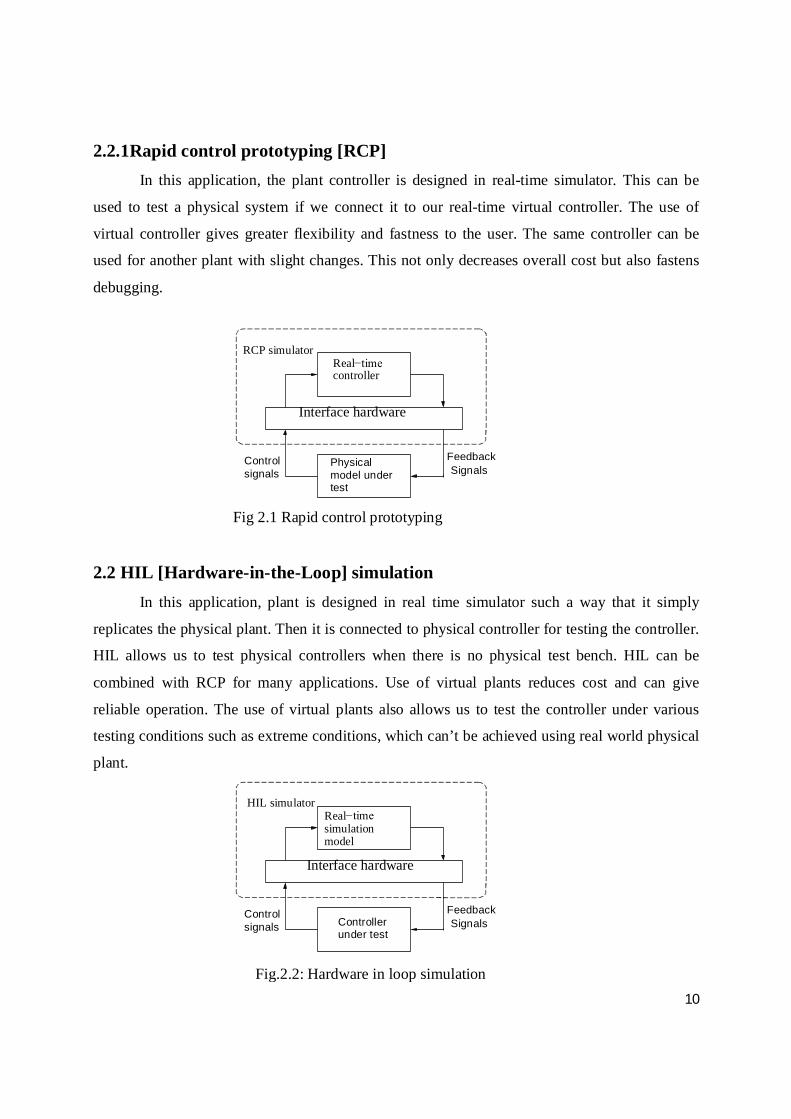
2.2.1Rapid control prototyping [RCP]

In this application, the plant controller is designed in real-time simulator. This can be

used to test a physical system if we connect it to our real-time virtual controller. The use of

virtual controller gives greater flexibility and fastness to the user. The same controller can be

used for another plant with slight changes. This not only decreases overall cost but also fastens

debugging.

Interface hardware

Fig 2.1 Rapid control prototyping

2.2 HIL [Hardware-in-the-Loop] simulation In this application, plant is designed in real time simulator such a way that it simply

replicates the physical plant. Then it is connected to physical controller for testing the controller.

HIL allows us to test physical controllers when there is no physical test bench. HIL can be

combined with RCP for many applications. Use of virtual plants reduces cost and can give

reliable operation. The use of virtual plants also allows us to test the controller under various

testing conditions such as extreme conditions, which can’t be achieved using real world physical

plant.

Interface hardware

HIL simulator Real−time simulation model

Interfacehardware

Control signals

Feedback Controller under test

Signals

RCP simulator Real−time controller

Control signals

Feedback Physical model under test

Signals

Fig.2.2: Hardware in loop simulation

11

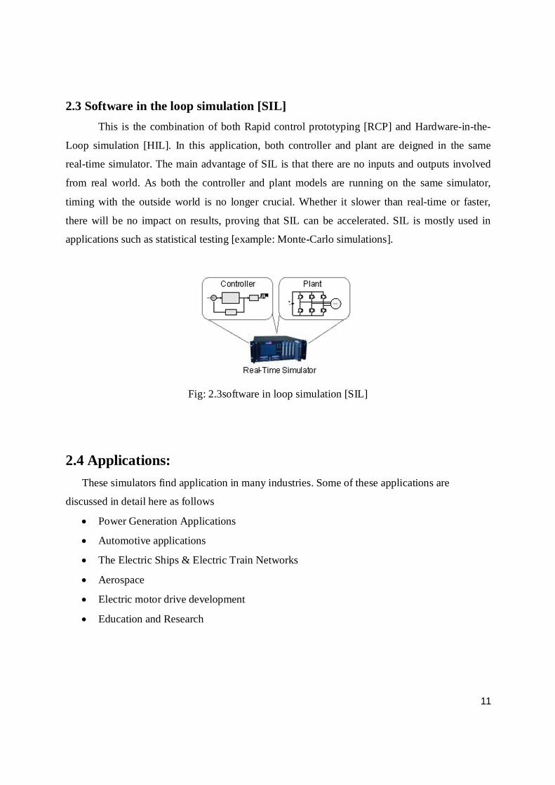
2.3 Software in the loop simulation [SIL] This is the combination of both Rapid control prototyping [RCP] and Hardware-in-the-

Loop simulation [HIL]. In this application, both controller and plant are deigned in the same

real-time simulator. The main advantage of SIL is that there are no inputs and outputs involved

from real world. As both the controller and plant models are running on the same simulator,

timing with the outside world is no longer crucial. Whether it slower than real-time or faster,

there will be no impact on results, proving that SIL can be accelerated. SIL is mostly used in

applications such as statistical testing [example: Monte-Carlo simulations].

Fig: 2.3software in loop simulation [SIL]

2.4 Applications: These simulators find application in many industries. Some of these applications are

discussed in detail here as follows

Power Generation Applications

Automotive applications

The Electric Ships & Electric Train Networks

Aerospace

Electric motor drive development

Education and Research

12

2.4.1 Power Generation Applications

These days testing of modern STATCOMs, HVDC links, (Static VAR Compensator)

SVCs, and FACTS devices under steady state and transient operating conditions, is a custom

while designing and after finishing the design. In order to cut back th e risks resulted in

conducting tests on physical networks we need real-time simulator for the network. HIL testing

should be conducted with a real-time prototype model successfully instead of using the real

physical controller .Many tests including both systematic and random have to be conducted

while testing the performance of a system under normal operating conditions as well as

abnormal operating conditions. This will help us in detecting the instabilities caused by

unwanted disturbances like the influence of other FACTS devices on our system that we are

testing.

While learning Protection and insulation coordination techniques for a huge power

system, people use statistical methods to deal with the inherent events, like finding the instant at

which the circuit breaker operates, or the point on the wave at which a fault occurs. We have

to identify, record and store the measure the quantities under several fault conditions by

conducting tests on occurrence of faults. These stored database can be used for future study

and analysis. T h e normal offline simulation software will be used while conducting

statistical study for the development of protection algorithms. If the hardware is finished we can

evaluate and develop the model using a real time simulator.

Fig.2.4: Multi-level VSC based STATCOM Fig.2.5: Real-time simulation of Renewable energy sources

13

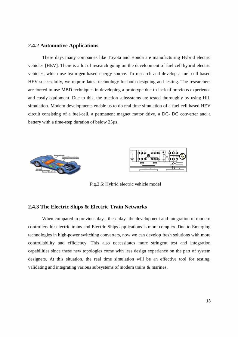
2.4.2 Automotive Applications

These days many companies like Toyota and Honda are manufacturing Hybrid electric

vehicles [HEV]. There is a lot of research going on the development of fuel cell hybrid electric

vehicles, which use hydrogen-based energy source. To research and develop a fuel cell based

HEV successfully, we require latest technology for both designing and testing. The researchers

are forced to use MBD techniques in developing a prototype due to lack of previous experience

and costly equipment. Due to this, the traction subsystems are tested thoroughly by using HIL

simulation. Modern developments enable us to do real time simulation of a fuel cell based HEV

circuit consisting of a fuel-cell, a permanent magnet motor drive, a DC- DC converter and a

battery with a time-step duration of below 25µs.

2.4.3 The Electric Ships & Electric Train Networks

When compared to previous days, these days the development and integration of modern

controllers for electric trains and Electric Ships applications is more complex. Due to Emerging

technologies in high-power switching converters, now we can develop fresh solutions with more

controllability and efficiency. This also necessitates more stringent test and integration

capabilities since these new topologies come with less design experience on the part of system

designers. At this situation, the real time simulation will be an effective tool for testing,

validating and integrating various subsystems of modern trains & marines.

Fig.2.6: Hybrid electric vehicle model

14

2.4.4 Aerospace

In aerospace applications, we may not need very low time-steps as that we use in power

generation applications. But the accuracy and repeatability of the simulation results are very

important for the purpose of safety. The aircraft manufacturers should maintain some standards

prescribed by the US-based RTCA (Radio Technical Commission for Aeronautics). Today’s

complex control systems in the aircraft can be designed and tested according to the above

mentioned standard. Thus the aerospace engineers need a higher precision testing and simulation

technologies that can ensure compliance. They should also consider the budget and built on time.

2.4.5 Electric motor drive development

The main advantage in developing the real time model of a motor drive is that we can

detect the defects while designing itself. If we find a problem after finishing of product, then we

have to spend more money to rectify it. Rapid prototyping methodology useful to the control

engineer in deploying control algorithms quickly and finding the problems. To perform this we

need an (Rapid control prototyping) RCP that is connected in a closed-loop with the actual

physical prototype of the drive which we want to control.

Fig 2.7: Electric motor drive model

Motor

15

2.4.6 Education and Research

The universities should be in update with the present technological revolution for making

the students and researchers to work on latest technologies. There are many new ways to teach

the students effectively. In order to provide them the practical experience which improves their

creativity, electronic simulators such as PSpice has been used as teaching tools from last few

years. They just build the required circuit in circuit editor and then simulate it to analyze the

results. But while studying the effect of variation in two or more parameters such as frequency

and duty cycle simultaneously, the offline simulation will take more time. In these situations,

simulation based on a real time simulator will be much effective teaching technique. Because the

real-time simulation gives the flexibility that the model parameter can be changed online means

during running. By using this tool we can provide the live feedback of the changes in the model

to the students, which will give them better understanding of the model.

16

Chapter 3

Requirements of Real-time simulation

17

Requirements for real-time simulation

There are certain requirements to be met to do real time simulation. They are as described below

Real-time capable operating system

In this case choose Linux as operating system because of its fast

performance. Another reason for selecting Linux is our Raspberry pi kit

supports Linux only

Hardware platform to run the simulation with external interface capability

For real time simulation, a hardware to do all the computations in

simulation with in the assigned time step is needed. Thus care should be

taken while selecting hardware simulator. There are many simulators in

market such as FPGA, MATLAB/SIMULINK. In this case Raspberry pi

chosen as the hardware simulator

Dynamic model of the system to be simulated

A mathematical model of the system to be simulated using ordinary

differential equations. In this case model of induction motor in linear

differential equations is designed.

Selecting a proper Numerical integration method and proper integration Time-step

To solve these differential equations a numerical integration method has to

be chosen out of many available methods. The selection depends on how

much accuracy is needed for the end user. The selection also depends on

the application area of the system and the capabilities of the hardware

simulator used.

Real time simulation software

A software platform to write the program and produce results has to be

selected. It should be capable of dynamic programming and memory

allocation. In this case the Python has been chosen as the simulation

software to program the code.

18

3.1 Introduction to Raspberry Pi

The Raspberry Pi is a very low-cost Linux minicomputer of nearly our palm size. It is

developed by the Raspberry Pi Foundation in the UK in 2011. The main purpose of designing the

Raspberry Pi is to provide programming skills to school students. Like our desktop CPU it has

also many components like processor, GPU, RAM, USB ports, Ethernet port and Audio and

video out channels. Hence it is also called as min computer.

The heart of our Raspberry Pi kit is the processor. It is equipped with Broadcom

BCM2835 SoC (system-on-chip). The SoC is a combination of CPU and GPU. The BCM2835 is

an ARM11 processor with a clock speed of 700 MHz . There are two models of raspberry pi

based on the Ram size. Our model is MODEL-B and is equipped with 512MB RAM. The

raspberry Pi doesn’t support WINDOW operating system. It only supports GNU/LINUX

operating system. There are different application based operating systems based on LINUX.

They are RASPBIAN, PIDORA, OPENELEC, RISC OS, RASPBMC. In this project

RASPBIAN was used as operating system.

Display The Raspberry Pi is equipped with two different types of video output ports such as

composite video, HDMI I/O port. Through composite port we can connect it a CRT (cathode ray

tube) TV. If we want best quality picture we can use HDMI port and it provides full HD

1920x1080 resolution. If we don’t have HDMI compatible display device, we can use converters

such as HDMI to DVI or HDMI to VGA converter.

Audio

The Raspberry Pi gives two ports for audio output. One is through HDMI port as it can

carry both video and audio signals. There is another separate audio port for 3.5mm jack.

19

Connecting Keyboard and Mouse The raspberry pi provides two (universal serial bus) USB 2.0 ports in order to connect our

Keyboard and mouse. Model A and Model B contains one and two USB ports respectively. And

the latest model, Model B+ contains 4 USB ports giving more access to the end user.

It has 26 GPIO (General Purpose Input output) low latency pins fixed on the top of the

board that allows low latency communication interfacing. Out of these pins some pins can be

used for two purposes. The GPIO facilitates the Pi to communicate with the other components

and circuits. These are also can be used to control a large electronic circuit. With the help of the

GPIO I/O port, we can sense temperature, operate servo motors and communicate with other

microcontrollers through any of the interfaces like SPI (serial peripheral interface) and I2C

(Inter-Integrated Circuit).

3.1.1 Interfacing We can communicate with Raspberry by four type of interfaces. They are:

one asynchronous serial interface (UART)

one serial peripheral interface (SPI)

two two-wire serial interfaces (commonly called

I²C)

Fig.3.1 The Raspberry Pi hardware kit

20

The Raspberry Pi can be able to interact with the outer real world. So it has been used in

a wide variety of applications starting from music machines and parent detectors to weather

stations and tweeting birdhouses with infra-red cameras. This can be programmed by using either

Python or Scratch. For our project, we are programming it in Python.

3.1.2 Applications of Raspberry Pi The Raspberry Pi can be used

As a Home theatre PC

As a Productivity machine to develop apps

As a Web server

As a microcontroller to interface with outer world

For each application we have to install corresponding Debian based operating system

3.2 Introduction to Python

Python is a programing language developed in the late 1980s. It is an object-oriented

language as it uses classes and methods in its programming. It comes under the high-level

language category, so the readability and understandability are more in this language. Python is

an interpreted language so the programs are need not to be converted into machine language and

are directly run by an interpreter. Python programs are not compiled into machine code but are

run by an interpreter. Thus the programs testing and debugging is easy and faster. It takes very

less time to write a program in python than in other languages like FORTAN and C because we

need not to compile and then link and then execute after each modification. Python is more

powerful and popular language than FORTAN. It is the one of the emerging programing

languages as many developments are going on it. However we need Python interpreter installed

in our computer in order to run a python program.

MATLAB and Python are quite similar as both are interpreter languages and high level

languages. Our Raspberry pi kit comes with inbuilt python software and comes with some

21

default libraries such as RpiGPIO.lib, math.lib, time.lib. But we have to download some other

libraries like scipy.lib, numpy.lib, matplotlib.lib...etc.

Python has got some advantages compared to other languages. They are as follows

Open source availability

o Python is an open-source software that means it is available for free of cost

Easy syntax:

o The syntax of python code is of short length and easier to learn

Greater supportability

o Python supports all the operating systems like Linux, Windows 7 and 8, Mac OS

Greater integrality

o Python Can be integrated with other programming platforms like C, JAVA,

C++…etc.

Concurrent processing

o Python has the ability to do concurrent processes effectively in the same program

thus making it one of the option for Real-time simulation

Object-oriented programming

o It uses classes and objects while addressing its code thus making the user to find

errors easily and allowing the user to program dynamically

High level language

o Python uses simple English expressions enabling the user to read and understand

the program easily. Learning python is easier than other programming languages

Numeric and scientific computation capabilities

o Python has a good scientific and math library with which we can do almost any

computation we want to do

22

3.3 Numerical integration methods Numerical integration or quadrature approximates the definite integral with a sum as

shown below. Statistically numerical integration is accurate than numerical differentiation.

The definite integral of form

푓(푥)푑푥

Can be written as a summation of

퐼 = 푊푓(푥 )

Where the nodal abscissas xi and weights Wi depend on the rule used for the numerical

integration method

There are two different categories of numerical integration one is Newton’s cotes

formulae and other is Gaussian numerical integration. The main point in Newton’s cotes

formulae is that abscissas are equally space by some distance h. the examples under this category

are Trapezoidal rule, Simpson’s rule. Where as in Gaussian numerical integration method

abscissa keeps changing to get best possible accuracy. Another advantage of Gaussian numerical

integration is that it allows singularities in integration

In this project Newton’s cotes formulae [ Euler explicit method] has been chosen as it is

simple to implement. There are many methods under this category based on the updating

formulae for Y-coordinate 푓(푥). We have discussed some important methods here. They are

23

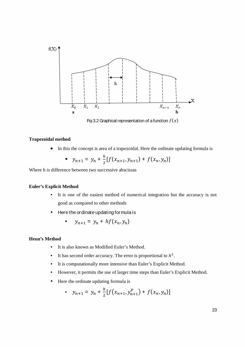
Trapezoidal method

In this the concept is area of a trapezoidal. Here the ordinate updating formula is

푦 = 푦 + [푓(푥 , 푦 ) + 푓(푥 ,푦 )]

Where h is difference between two successive abscissas

Euler’s Explicit Method

• It is one of the easiest method of numerical integration but the accuracy is not

good as compared to other methods

• Heretheordinateupdatingformulais • 푦 = 푦 + ℎ푓(푥 ,푦 )

Heun’s Method

• It is also known as Modified Euler’s Method.

• It has second order accuracy. The error is proportional to ℎ .

• It is computationally more intensive than Euler’s Explicit Method.

• However, it permits the use of larger time steps than Euler’s Explicit Method.

• Here the ordinate updating formula is

• 푦 = 푦 + [푓 푥 , 푦 + 푓(푥 ,푦 )]

Fig 3.2 Graphical representation of a function 푓(푥)

24

RUNGE-KUTTA Method

Here the integration formulae is

푦 = 푦 +ℎ6 [푝 + 2푝 + 2푝 + 푝 ]

푥 = 푥 + ℎ

푝 = 푓(푥 ,푦 )

푝 = 푓 푥 +ℎ2 ,푦 +

ℎ2 푝

푝 = 푓(푥 +ℎ2 ,푦 +

ℎ2 푝 )

푝 = 푓(푥 + ℎ,푦 + ℎ푝 )

Adams-Bash forth Method

• The slope used is the weighted average of the slope at the previous time point, and the

one before that

• Second order accuracy

• How to start the integration at n = 0?

• One way: Use Euler’s method to calculate the value of yi(−1)

• The formula is

yi (n+1)=yi (n)+T(1/2 )* f i (y1(n),..,yN(n))− (3 / 2) * f i (yi (n−1),..,yN (n-1))

Simpson’s 1/3 rule

Here the integration formula is

∫ f(X)dx= [f (푋 ) + 4 f (푋 ) + 2 f (푋 ) + 4 f (푋 ) +······ + 2 f (푋 ) + 4 f (푋 ) + f (푋 )]

Simpson’s 3/8 rule

Here the integration formula is

∫ f(X)dx= [f (푋 ) + 3 f (푋 ) + 3 f (푋 ) + f (푋 )]

25

3.4 Induction motor modeling The dynamic model of a physical system is usually developed as a set of first-order

ordinary differential equations, perhaps nonlinear. The model development is the result of the

application of basic physical laws to describe the system dynamic behavior. In general the model

development always involves making simplifying assumptions. Some of these assumptions may

be obvious. Others will be more subtle. When one uses a dynamic model of any system, it is very

important to have a clear idea of what to expect, and what not to expect, from it.

The essential point here is that in developing the dynamic model of any physical system,

we are faced with a trade-off between exactness and usability. The model may be very exact, but

it may be so complicated that it may be difficult to use. On the other hand, the model may be

very easy to use, but it may be trivial to the point of uselessness. It is important to identify an

appropriate set of assumptions in developing the dynamic model of a physical system. This is

also true of dynamic models of electric machines. Here the dynamic model of an induction motor

has been implemented.

The model development process for a rotating electric machine typically goes through the

following steps.

Step 1: Derive expressions for the machine inductances based on geometry and winding

distribution.

Machine inductance expressions are derived by describing the machine winding layout in terms

of winding functions. These functions enable machine windings to be described mathematically.

Step 2: Set up equations for winding flux linkages of the form

λi=ΣLkik

Step 3: Write down the machine electrical equations in the form

vi =λ˙ i+ Riii

Steps 2 and 3 describe the electric circuit equations of the machine by relating the winding

terminal voltages to resistive voltage drops and rates of change of flux linkages

Step 4: Simplify the form of the equations using a transformation of variables.

26

For AC machines, the electric model of the machine after Step 3 is often in a very complicated

form. This is because of two main reasons:

There is mutual coupling between all pairs of windings.

The mutual coupling between stator and rotor windings is position-dependent.

A transformation of variables helps in simplifying the electrical equations.

Step 5: Derive an expression for the rotor torque Te based on the electrical variables.

Step 6: Write down the machine mechanical equation in the form

휔 =푇 − 푇

퐽 … … … … … … … … … … … … … Eq(3.1)

Where ωr is the rotor speed, TL is the load torque, and J is the rotational inertia. After these steps,

we will have a set of first order ordinary differential equations that describe the

electromechanical behavior of the machine. This set of equations is our machine dynamic model.

The dynamic plant model is thus made up of a number of first-order ordinary differential

equations and algebraic equations. By Starting from the given initial conditions, the evolution of

the system states can be determined by numerically integrating the differential equations

These days most widely used motors are induction motors because of its simple operation

and rugged construction. It is basic component foe an Electric drive. Induction motor can be

modeled in many ways based on the control method used. The Transient analysis of induction

motor gives better understanding of the machine. For a given model of induction motor, one can

analyze it in many ways depending on the reference frame chosen.

All the analysis has been based on the dynamic representation or D-Q equivalent circuit

of induction motor and is done in rotating reference frame. The differential equations with

respect to stator reference frame can be described as follows:

The stator voltage equations are as described below:

푣 = 푅 푖 +푑휑푑푡

−푤 휑 … … … … … … … … … … … … … Eq(3.2)

27

푣 = 푅 푖 +푑휑푑푡

+ 푤 휑 … … … … … … … … … … … … … Eq(3.3)

For a squirrel cage induction motor, the rotor is always short-circuited, so 푣 = 0and푣 = 0

Hence the rotor voltage equations are as described below:

푣 = 0 = 푅 푖 +푑휑푑푡

− (푤 −푤 )휑 … … … … … … … … … … … … … Eq(3.4)

푣 = 0 = 푅 푖 +푑휑푑푡

+ (푤 −푤 )휑 … … … … … … … … … … … … … Eq(3.5)

Where‘d’ is corresponding to direct axis and ‘q’ is corresponding to quadrature axis,

푣 = 푑 − axisstatorvoltage

푣 = 푞 − axisstatorvoltage

푣 = 푑 − axisrotorvoltage

푣 = 푞 − axisrotorvoltage

푅 = statorresistance

푅 = rotorresistance

푤 = angularvelocityofrotor

Assume 휑 ,휑 arefluxlinkages of stator corresponding to d-axis and q-axis respectively and

휑 ,휑 arefluxlinkagesofrotorcorrespondingtod− axisandq − axisrespectively. Then

the flux linkage equations are as described below:

휑 = 퐿 푖 + 퐿 푖 … … … … … … … … … … … … … Eq(3.6)

휑 = 퐿 푖 + 퐿 푖 … … … … … … … … … … … … … Eq(3.7)

휑 = 퐿 푖 + 퐿 푖 … … … … … … … … … … … … … Eq(3.8)

휑 = 퐿 푖 + 퐿 푖 … … … … … … … … … … … … … Eq(3.9)

Where

퐿 = 푆푡푎푡표푟푠푒푙푓푖푛푑푢푐푡푎푛푐푒

28

퐿 = 푆푡푎푡표푟푠푒푙푓푖푛푑푢푐푡푎푛푐푒

퐿 = 푀푢푡푢푎푙푖푛푑푢푐푡푎푛푐푒

푤 = angularvelocityofreferenceframe

From above equations, we can express currents in terms of flux linkages as

푖 =퐿

퐿 퐿 − 퐿휑 −

퐿퐿 퐿 − 퐿

휑 … … … … … … … … … … … … … Eq(3.10)

푖 =퐿

퐿 퐿 − 퐿휑 −

퐿퐿 퐿 − 퐿

휑 … … … … … … … … … … … … … Eq(3.11)

푖 =퐿

퐿 퐿 − 퐿휑 −

퐿퐿 퐿 − 퐿

휑 … … … … … … … … … … … … … Eq(3.12)

푖 =퐿

퐿 퐿 − 퐿휑 −

퐿퐿 퐿 − 퐿

휑 … … … … … … … … … … … … … Eq(3.13)

The electromagnetic torque of the machine can be expressed as

푇 =3푃4퐿 [푖 푖 − 푖 푖 ] … … … … … … … … … … … … … Eq(3.14)

Where, P is number of poles andT is the electromagnetic torque.

By neglecting mechanical damping the relation between torque and rotor speed can be related as

= (푇 − 푇 ) … … … … … … … … … … … … … Eq(3.15)

Where푇 = Loadtorque

The ordinary differential equations that represent the dynamic model of induction motor are

given below

푑휑푑푡

= 푣 −푅 퐿

퐿 퐿 − 퐿휑 +

푅 퐿퐿 퐿 − 퐿

휑 + 푤 휑 … … … … … … Eq(3.16)

푑휑푑푡

= 푣 −푅 퐿

퐿 퐿 − 퐿휑 +

푅 퐿퐿 퐿 − 퐿

휑 −푤 휑 … … … … … … Eq(3.17)

29

푑휑푑푡

= −푅 퐿

퐿 퐿 − 퐿휑 +

푅 퐿퐿 퐿 − 퐿

휑 + (푤 −푤 )휑 … … … … … … Eq(3.18)

푑휑푑푡

= −푅 퐿

퐿 퐿 − 퐿휑 +

푅 퐿퐿 퐿 − 퐿

휑 + (푤 −푤 )휑 … … … … … … Eq(3.19)

= (푇 − 푇 )… … … … … … … … … … … … . . Eq(3.20)

Upon integrating these five differential equations eq (3.16), (3.17),(3.18),(3.19),(3.20) in each

iteration using a suitable numerical integration method, we have to update them with the

previous results.

30

Chapter 4

Real-time simulation using Raspberry Pi

31

Real-time simulation using Raspberry Pi

For running simulations on the Raspberry Pi board, system performance is a difficulty.

The ARM core includes a single-precision floating-point unit that helps for environment models

engineered on mathematical algorithms. If performance is lacking by a tiny low margin, the

Raspberry Pi will safely be overclocked by concerning 10 to 20 percent. Some boards can be

overclocked by more than 50 percentage.

With a specific end goal to minimize cost, we didn't utilize add-on sheets for extra I/O

channels. Rather, we attempted to get by with simply the bare Raspberry Pi. This represents an

extra challenge: The Raspberry Pi has no usable Digital to Analog and Analog to Digital

converters. Its two inward PWM generators are connected to the earphone jack by means of an

audio quality RC filter. This may be utilized in some cases, yet we disregarded that plausibility

to prevent signal integrity issues.

Raspberry Pi is a mini computer that runs on LINUX operating system. It is compatible

with many Debian based operating systems such as RASPBIAN, PIDORA, OPENELEC, ARCH

LINUX, and RISC OS. Etc. these operating systems are application specific. For our application,

we choose RASPBIAN as our operating system. We are designing the induction motor model in

raspberry pausing python. As Raspberry Pi consists of 26 GPIO pins for interfacing with the

outer world. Raspberry provides various types of interfacing such as serial peripheral interface

(SPI) and inter-integrated circuit (I2C).

Below here is the list of Raspberry Pi peripherals that are useful for our real-time simulation. We

are planned to do HIL type Real-time simulation using our Pi kit.

Timers

Interrupt controller

GPIO

32

The Timer peripheral in BCM2835 chip consists of 4 32-bit timer channels and one 64-

bit counter (updated at every 1us rate). Every channel has been provided with an output compare

register that compares up to 32 least significant bits. Whenever the compared values are

matching, the timer peripheral produces a signal for indicating the match. This signal is fed into

the interrupt controller. The interrupt service routine will read the compare register output and

adds an appropriate offset for the next timer clock. In order to get accurate time interval for

integration time step, following process should be followed.

Read a value from the counter into some variable

Add an offset equivalent to time delay required to the variable

keep branching back into the same code until the counter value and the variable value

matches

The main objective is to test the designed model with the help of a real world controller

such as an accelerometer or an LVDT. As all the GPIO pins are digital pins, there is requirement

of a DAQ card (NI-DAQ 6009) for analog to digital conversion. But while accessing the GPIO

pins, some problems came into picture. For middle and higher range frequencies, the output of

the pins is toggling from HIGH state to LOW state unexpectedly. So the analog value is keep

changing within 10 Nano seconds. So the DAQ card option also went wrong as the obtained

results are not reliable.

Later the other types of interfacing Serial peripheral interfacing and I2C interfacing (one

wire communication) have been tried. The Arduino UNO board is connected to the Raspberry Pi

kit using SPI interfacing. The Arduino acts as the controller to the real-time induction model

designed in our Pi kit. But some errors resulted. The reason is that the kit is not recognizing the

SPI or I2C device. Now the results has to be displayed in real time using python plot commands.

For that install matplotlib.lib library as it won’t come default with the kit. But remind that it is a

third party software not from official website.

33

A model is designed by programming such that it updates the results at the end of each

time-step, which is an important feature in real-time simulation. All the state variables are

defined in an array (in python language we call it a List) of floating numbers. By selecting a time

step of 0.001 sec, simulation has been carried out. There is no errors resulted but a warning

showing that the memory is full and there are too many variables to proceed displayed on the

control window. By decreasing the time-step to 0.01 sec, simulation has been carried out but still

the same error appeared. Then an offline simulation of induction motor using Pi kit. The results

are of pretty accurate. By comparing them with the MATLAB results, the results obtained are

nearly same as the MATLAB results. The results are attached in the appendix page.

4.1 Simulation results:

휔e=376.99 rad/s, 푟 = 0.435 Ω, 푟 = 0.816 Ω, xs= 26.88 Ω, J=0.089 Kg/m2, T=0 Nm

Fig.4.1: The electromagnetic torque vs rotor speed of 3-phase induction motor

Fig.4.2: The stator current of 3-phase induction motor Time In seconds

34

Fig.4.3: The rotor current of 3-phase induction motor

Fig.4.4: The electromagnetic torque of 3-phase induction motor

Fig.4.5: The rotor speed of 3-phase induction motor

Time In seconds

Time In seconds

Time In seconds

35

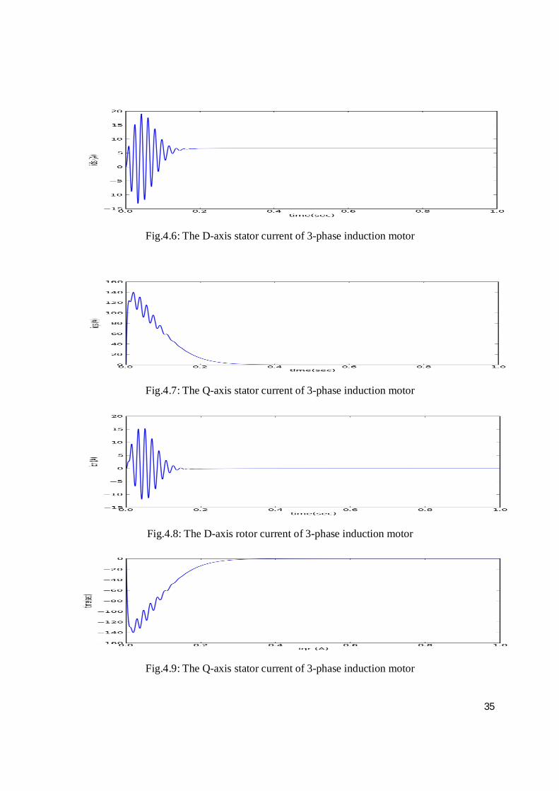
Fig.4.6: The D-axis stator current of 3-phase induction motor

Fig.4.7: The Q-axis stator current of 3-phase induction motor

Fig.4.8: The D-axis rotor current of 3-phase induction motor

Fig.4.9: The Q-axis stator current of 3-phase induction motor

36

Chapter 5

Real time simulation using MATLAB

37

Real time simulation using MATLAB

Nowadays MATLAB is a very powerful simulation software and is widely used in

engineering, research and educational purposes. Doing real-time simulation in MATLAB

requires better programming knowledge. The real time simulation in MATLAB gives better

understanding of our system. The real time simulation can be done in two ways in MATLAB.

One way is through programming in MATLAB editor and the other way is through

MATLAB/SIMULINK. In this project this is accomplished by normal programming. However

one can done it in SIMULINK also but time didn’t permitted us to do it. So there won’t be any

discussion about SIMULINK in this thesis. However offline simulation of induction motor is

done in Simulink and the model, results are discussed in Appendix.

First of all, in order to do real time simulation one needs a real timer in the real time

simulator hardware. In conventional PC there is inbuilt timer so there is no need to worry about

it. There is need to have some idea about MATLAB timer programming for MATLAB

simulation. We need to take into consideration the processor clock speed. For that one can use

the command “cputime” in MATLAB.

The selection of the integration time-step is the main considerate in doing real time

simulation. The tine step to be chosen such a way that it should be greater than the maximum

time taken by the system for one iteration. To calculate this maximum time taken, one has to

program in MATLAB to start and stop the stopwatch. For this purpose commands such as “tic”

to start the timer and “toc” to stop the timer are useful.

In real time simulation, each iteration should take similar time that is provided by the

user. But depending on the capacity of the processor, the real-time software used and complexity

of the system the time taken for each iteration may be different. One need to program the model

by taking all these factors into consideration. The processor should be put on idle mode when the

time taken is less than the time-step provided. In order to get accurate time interval in each

iteration, one need to start the timer at the starting of each iteration and stop it at the end of the

iteration. By using this period of time one can decide how much time we have to suspend the

38

processor so that the result will be available at the next time-step, which is mandatory in real-

time simulation.

The program can be put into wait state by two ways. First is by stopping the processor for

that interval and the second way is by running an empty loop until total iteration time is equal to

the time-step provided. In MATLAB, by using “pause” function, the processor can be stopped

for some time. This stop time for the processor is nothing but the difference between the fixed

time-step provided and the iteration time of that particular iteration. However the “pause”

function precision is in tens of mille seconds only. So better to go for the second alternative

which is running an empty loop.

pause((Fixed time step provided)-(iteration time for that iteration))

In generating an empty loop one has to keep reading the stopwatch time and when it

reaches the wait time, get out of the loop by using the “break” function. By this way one can get

accurate time interval in the order of micro seconds.

For integration in MATLAB, technicians normally use “odeint” function by mentioning

the initial states, the start time, end time and the time step. The program directly gives the results

after all the iterations are completed. Technician don’t have control on any iteration and he can’t

to do anything in between two successive iterations. However in order to do real-time simulation

one has to update the state variable values in the real-time plot, which can’t be achieved simply

by using “odeint” function. Thus a custom made integration function is needed for the real-time

simulation.

While plotting the real-time plot one has to make use of some functions in MATLAB.

The first thing is to hold the plot with fixed axes until total simulation is completed. For this

purpose the “hold” MATLAB function is useful. The next thing updating the ordinate value with

the present iteration result and also keeping the previous data. This can be achieved by using the

“drawnow” MATLAB function. This is how one can plot a real-time plot.

39

In real time simulation the engineer have to design a custom made integration function in

order to update the state variables in each time step and stop the process if the integration is

completed faster than the provided simulation time-step. This can also be achieved in another

way without using custom made integration function. To accomplish this one can use the inbuilt

MATLAB function “odeint”. This can be done by taking another time-step of value smaller than

our provided time-step for the integration purpose in one iteration. And the end value in this

iteration is assigned to the starting value of the next iteration. And if all this process is completed

before the simulation time-step, then the program is put into idle mode for that extra time. So

that engineer will have full control over each and every iteration of the simulation. That means,

the state variable is updating in each iteration with the previous iteration state variables

indirectly. One will get a clear idea, if he carefully observe the program.

5.1 Simulation results

Real-time simulation has been done on an induction motor using MATLAB with the

below mentioned machine ratings and the results are shown below. The simulated response for

the system in 5 seconds is shown here.휔e=376.99 rad/s, 푟 = 0.435 Ω, 푟 = 0.816 Ω, xs= 26.88 Ω,

J=0.089 Kg/m2, T=0 Nm

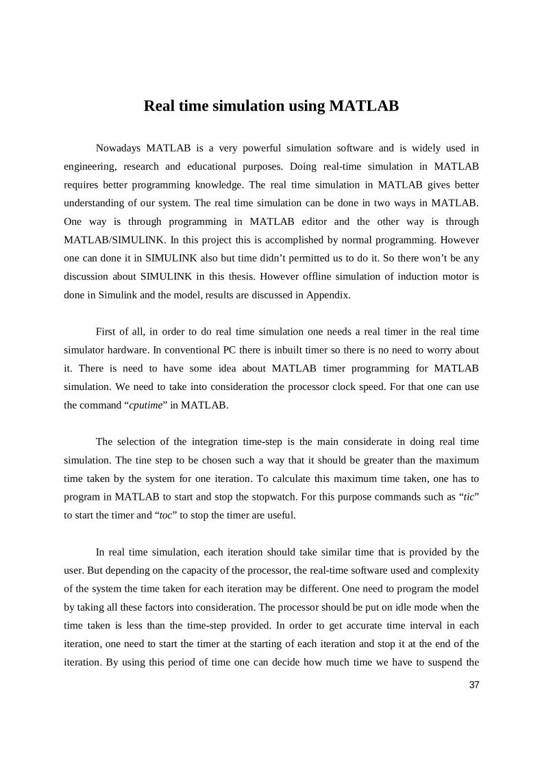
Stator currents:

Figure 5.1 and fig: 5.2 shows variation of the d-axis stator current the q-axis stator current with time. Fig 5.3 shows the comparison between d-axis and q-axis stator currents

Fig.5.1: the D-axis stator current of 3-phase induction motor

40

Fig.5.2: the Q-axis stator current of 3-phase induction motor

Fig 5.3: Comparison between D-axis and Q-axis stator currents of 3-phase induction motor

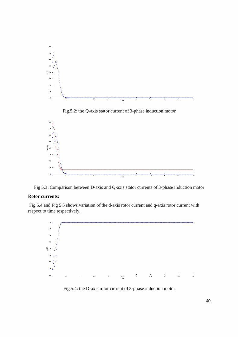
Rotor currents:

Fig 5.4 and Fig 5.5 shows variation of the d-axis rotor current and q-axis rotor current with respect to time respectively.

Fig.5.4: the D-axis rotor current of 3-phase induction motor

41

Fig.5.5: the Q-axis rotor current of 3-phase induction motor

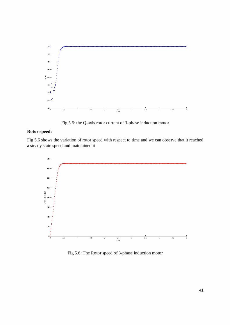
Rotor speed:

Fig 5.6 shows the variation of rotor speed with respect to time and we can observe that it reached a steady state speed and maintained it

Fig 5.6: The Rotor speed of 3-phase induction motor

42

Torque vs Speed

Fig 5.7 shows variation of torque with respect to rotor speed

Fig 5.7: the electromagnetic torque vs rotor speed of 3-phase induction motor

43

Chapter 6

Conclusion &

Bibliography

44

6.1 Conclusion

Modern power systems are implementing power electronic converters, so there are many

studies are going on superfast, flexible and reliable real-time simulators. There is a lot of

research going on implementation of low-cost real-time simulators. This thesis describes how the

real-time simulation on Raspberry Pi has been done and associated problems with possible

solutions. This thesis provides a platform for low cost real-time simulator. In this thesis real-time

simulation using MATLAB has also been done and results are displayed. The simple steps

involved in this process are discussed in this paper elaborately. This thesis also describes the

essence and applications of real time simulation.

6.2 Future work

In future there is scope for other alternatives of low-cost real-time simulators “such as

Arduino. There is lot of scope in this field as many developments are going on in design of

microcontrollers and many advanced techniques are coming out.

6.3 Bibliography

[1] “The What, Where and Why of Real-Time Simulation” J. Bélanger, Member, IEEE, P. Venne,

Student Member, IEEE, and J.-N. Paquin, Member, IEEE

[2] “Hardware-Based Real-Time Simulation”, Jörg Walter, Maher Fakih, and Kim Grüttner

OFFIS Institute for Information Technology, Oldenburg, Germany

[3] “Induction motor modelling for vector control purposes”,Mircea Popescu, Helsinki

University of Technology Department of Electrical and Communications Engineering

[4]“Numerical Methods in Engineering with PYTHON” by Jaan Kiusalaas

45

[5] “Simulink / MATLAB Dynamic Induction Motor Model for use in Undergraduate Electric

Machines and Power Electronics Courses”, A.W. Leedy, Member, IEEE Department of

Engineering & Physics Murray State University

[6] www.docs.python.org

[7] www.codecademy.com/en/tracks/python

[8] www.tutorialspoint.com/matlab

[9]https://plot.ly/matlab/streaming-tutorial

[10]http://in.mathworks.com/matlabcentral/answers/87466-real-time-plot-from-streaming-data

[11] www.raspberrypi.org

[12] www.adafruit.com

[13] www.youtube.com/matlabtutorials

46

APPENDIX-A

Offline Simulation of induction motor using MATLAB/SIMULINK

An offline simulation of a three phase induction motor is conducted in MATLAB/SIMULINK and the results are shown here

Fig i: SIMULINK block diagram of 3-phase induction motor

Fig ii: The inside architecture of the SIMULINK block of 3-phase induction motor

47

Simulation Results:

Stator phase currents

Fig iii: The stator current of 3-phase induction motor

Rotor phase currents

Fig iv: The stator current of 3-phase induction motor

48

Torque

Fig v: The electromagnetic torque of 3-phase induction motor

Speed

Fig vi: The rotor speed of 3-phase induction motor

49

Torque vs Speed

Fig vii: The electromagnetic torque vs rotor speed of 3-phase induction motor