Real-time verification of wireless home networks using bigraphs with sharing Muffy Calder 1a , Alexandros Koliousis b , Michele Sevegnani a , Joseph Sventek a a School of Computing Science, University of Glasgow, UK b Dept of Computing, Imperial College London, UK Abstract Home wireless networks are difficult to manage and comprehend because of evolving locality, co-locality, connectivity and interaction. We define formal models of home wireless network infrastructure and policies and investigate how they can be used in a network management system designed to provide user-oriented support. We model spatial and temporal behaviour of network interactions and user-initiated network policies and define an online framework for generation of models from network and user-initiated events. The models are expressed in an extension to Milner’s bigraphical reactive systems. Analysis of the models is carried out in real-time by a bespoke bigraph reasoning system based on checking predicates, which is encoded as bigraph matching. Real-time model generation and analysis is implemented on the experimental Homework system router and trialled with synthetic and actual network data. Keywords: network management, verification, bigraphical reaction systems, bigraphs with sharing, runtime model generation, bigraph matching 1. Introduction Wireless home networking is notoriously difficult to install and manage, es- pecially for non-expert users. The Homework network management system [1] is an experimental system designed to provide user-oriented support in home wireless local area network (WLAN) environments. The Homework system is much more than a user interface for existing network infrastructure. It provides new network architectures that take into account the sociotechnical nature of home networking. For example, devices are brought into the home by fam- ily and friends, and users define policies for explicit management and access. It also encompasses new approaches to infrastructure measurement and mon- itoring and user focussed computational models for modelling and analysis in support of both design and user experience. In particular, the Homework sys- tem is a platform from which we can investigate how formal models can be used 1 Corresponding author. e-mail: Muff[email protected]. Preprint submitted to Elsevier August 5, 2013
Transcript
Real-time verification of wireless home networks usingbigraphs with sharing
Muffy Calder 1a, Alexandros Koliousisb, Michele Sevegnania, Joseph Sventeka
aSchool of Computing Science, University of Glasgow, UKbDept of Computing, Imperial College London, UK
Abstract
Home wireless networks are difficult to manage and comprehend becauseof evolving locality, co-locality, connectivity and interaction. We define formalmodels of home wireless network infrastructure and policies and investigatehow they can be used in a network management system designed to provideuser-oriented support. We model spatial and temporal behaviour of networkinteractions and user-initiated network policies and define an online frameworkfor generation of models from network and user-initiated events. The modelsare expressed in an extension to Milner’s bigraphical reactive systems. Analysisof the models is carried out in real-time by a bespoke bigraph reasoning systembased on checking predicates, which is encoded as bigraph matching. Real-timemodel generation and analysis is implemented on the experimental Homeworksystem router and trialled with synthetic and actual network data.
Keywords: network management, verification, bigraphical reaction systems,bigraphs with sharing, runtime model generation, bigraph matching
1. Introduction
Wireless home networking is notoriously difficult to install and manage, es-pecially for non-expert users. The Homework network management system [1]is an experimental system designed to provide user-oriented support in homewireless local area network (WLAN) environments. The Homework system ismuch more than a user interface for existing network infrastructure. It providesnew network architectures that take into account the sociotechnical nature ofhome networking. For example, devices are brought into the home by fam-ily and friends, and users define policies for explicit management and access.It also encompasses new approaches to infrastructure measurement and mon-itoring and user focussed computational models for modelling and analysis insupport of both design and user experience. In particular, the Homework sys-tem is a platform from which we can investigate how formal models can be used
iteratively and interactively to contribute to the question “is the proposed net-work infrastructure fit for purpose”, and more generally, if and how seamfullyexposing models of infrastructure and user behaviour to those being modelledis useful and can be carried out in real-time, without interruption or delay tothe network management system.
The aim of this paper is to define suitable formal models of the infrastructureand policies and to investigate how they can be used in an extension to the basicHomework network management system.
1.1. The standard Homework system
The Homework system architecture consists of three complementary planes:data, signalling, and information. We focus on the last, which is a monitoringapplication that makes available information about network set-up, managementand measurement. It uses a stream database to record (raw and derived) events.Events include network behaviours such as detecting that a new machine hasjoined the network, resulting in new links and granting a DHCP lease, and user-initiated behaviours such a enforcing or dropping a policy. Policies are definedby users through a novel user interface that allows drag and drop, comic-stripstyle interaction (see [2]). Typically, policies forbid or allow access to networkresources; for example, a policy might block UDP and TCP traffic from a givenwebsite, or restrict internet access for certain users during given time periods.
1.2. Modelling wireless network management
Locality, co-location, interaction, connectivity, and user-perceived events arekey aspects of user-oriented home networking. We require models that exposethese aspects, and their temporal evolution, to both end users and system de-velopers, and permit computation and analysis of properties in real-time. Whilevarious formalisms might fit these criteria to a greater or lesser extent, we pro-pose that bigraphs with sharing, an extension of Milner’s universal process al-gebra that encapsulates both dynamic and spatial behaviour [3], fit all thesecriteria particularly well. Specifically, bigraphical reactive systems (BRS) arewell suited to the problem because a) the (human-oriented) graphical form pro-vides an intuitive representation of locality, co-locality, and connectivity, b)there is an explict representation of user-perceived events by rewrite rules andc) there is a (machine readable) algebraic form for computation and verificationof properties.
In our models, each BRS consists of a set of bigraphs that describes spatialand communication relationships between machines and entities in the network,and a set of bigraphical reaction rules that define how the bigraphs can evolveover time. We have extended the basic formalism of BRS to bigraphical re-active systems with sharing, to permit effective and intuitive representation ofspatial locations that can overlap2. This extension is particularly relevant to
2Henceforth we refer to this extension simply as BRS.
2
Network
Stream database
Bigraph analysis
Logfiles
Bigraph encoder
feedback
feedback
Policy enforce/drop
Raw network traffic
updated bigraph
events
Figure 1: Real-time model generation, analysis and feedback in the Homeworksystem.
our requirements, since multiple, overlapping signals are fundamental to wirelessnetworks.
1.3. Real-time model generation, analysis and feedback in Homework
In our extension to the Homework system, models are generated from eventsrecorded in the information plane and analysed without interruption or delayto the network management system.
The system is depicted in Figure 1. As we have indicated above, the Streamdatabase is part of the standard Homework management system; all networkand policy events are recorded as streams of tuples in the database. The Bi-graph encoder component is new, and it encodes events as bigraphical reactionrules. The Bigraph analysis component is also new, and it has two roles. First,it generates the bigraphical representation of the current configuration of theWLAN, according to the sequences of reaction rules received from the Bigraphencoder. Second, it analyses the current configuration by checking properties,for example, whether or not a configuration violates a user-invoked access con-trol policy. Properties are expressed as predicates that are encoded as instancesof bigraph matching. The results are logged and can be fed back to the system,or to the user, using the graphical notation of bigraphs as explanation. Thiswork flow is carried out in real-time, hence we refer to our approach as real-timeverification.
While our long-term motivation is to aid users in their understanding of thestate of their system (e.g. when and why it is “broken”), and to give feedback todevelopers about user experiences, in this paper we concentrate on the technicaldetails of the representations of networks and policies and the analysis systemitself.
3
1.4. Overview of paper
The main focus of this paper is to describe the bigraphical representationsof networks topologies, the events that modify topologies and the access controlpolicies, and how to represent and check predicates on bigraphs within theruntime system.
The contributions of the paper are the following:
• representations of network topologies as bigraphs and network events (suchas a machine leaving and joining a network) as bigraphical reaction rules,
• representations of access control policies that forbid and allow behavioursas bigraphical reaction rules that constrain network evolutions,
• new reasoning techniques for predicates over bigraphs, encoded as in-stances of bigraph matching and implemented using a SAT solver,
• a solution for the problem of how to check for the non-existence of patternsin bigraphical reaction rules, and how to reason about topologies witharbitrary numbers of machines and communication channels, by taggingand untagging entities,
• on-line generation of bigraphical reactive system models from the currentnetwork topology and activated policies, as recorded in the Homeworkinformation plane, and
• empirical evidence demonstrating that generation and analysis of bigraphmodels can be carried out in real-time within the Homework system.
The paper is organised as follows. Section 2 contains an informal introduc-tion to the bigraph notation, bigraphical reactive systems and bigraph matching.In Section 3 we describe how network topologies are represented as bigraphicalsystems and how network events, such as moving in and out of the router’srange, and granting and revoking of leases, are encoded as reaction rules; inSection 4 we show how predicates are encoded as bigraphs, and thus can bechecked by bigraph matching. In Section 5 the rules and predicates definedin Section 3 are used to generate sequences of models in real-time. Section 6describes how policies that forbid and allow behaviour are represented as bi-graphical reaction rules and how they constrain network evolutions. In Section7 we describe how policy events such as enforce a policy, drop a policy or checka policy, are encoded as reaction rules, and we discuss the interplay between the(representations of) network and policy events. In Section 8 we show in detailhow a bigraphical model of a WLAN is updated according to the stream ofnetwork and policy events generated in real-time. Section 9 discusses the role ofstate predicates in the analysis of network configurations and compliance withpolicies; in Section 10, we give an overview of the implementation. A discussionof the overall approach and the role of the bigraph abstraction is in Section 11and related work is reviewed in Section 12; we conclude in Section 13.
4
Router R
Machine M1
Machine M1
signal
Router R
signal
Figure 2: Simple WLAN with one machine and a router.
2. Bigraphs with sharing
In this section we give an informal overview of BRS, with some examples.The overview contains sufficient detail for this paper; a concise semantics of bi-graphs with sharing is defined in [4]. Details of standard BRS (without sharing)are in [3].
A bigraph has a graphical and an algebraic form. In this paper, we use bothforms, but primarily the graphical form. In the graphical form, an entity (realor virtual) is encoded by a node (oval or circle). Spatial placement of nodes isdescribed by node nesting, which we have extended to directed acylic graphs.Thus, nodes can be placed in the intersection of other nodes. Each node isassigned a control. Interaction between nodes is represented by an edge called alink that connects ports. Each node can have zero, one or many ports, indicatedby bullets. They can be thought of as sockets into which links can be plugged. Adashed rectangle denotes a region of adjacent parts of the system. A grey squareindicates a site, which encodes part of the model that has been abstracted away.A link may be only partially specified, in which case it connects ports with aname. Name closure /xA is used to disallow connections on name x in bigraphA.
As an example, consider the WLAN depicted in Figure 2: there is one ma-chine and a router in the network, each associated with a signal.
This network is represented as a bigraph in Figure 3. There are threecontrols M1, S, and R; the two signals (of the machine and the router) arerepresented by the nodes of control S, the router is indicated by the node ofcontrol R and the machine is represented by the node of control M1. There arethree links: a link between machine M1 and its signal, a link between routerR and its signal, and a link between machine M1 and router R. There are nonames in this bigraph.
The capabilities of a bigraph to interact with the external environment aregiven in its interface. For example, we write A : 1 → 〈2, {x, y}〉 to indicate
5
S
M1
R
S
Figure 3: Bigraph representation of simple WLAN with one machine and arouter.
that A has one site, two regions and the names x and y. Controls and linksin a bigraph are classified by means of sorts (ranged over by a, b, ...) and aformation rule defines sorting properties a bigraph has to satisfy. For example,in a WLAN representation, a typical formation rule would be: an R node isalways contained in an S node (i.e. a router has a signal). A sort may be a
disjunction, which we denote as follows: ab means that a node can have sort a orb. The interface of a sorted bigraph is expressed as follows: A : a→ 〈bb, {x, y}〉.The notation indicates that the site has sort a and the two regions have sort b.
The structure of a bigraph can also be specified in algebraic form by com-bining elementary bigraphs and bigraphical operations. A summary is givenin Table 1. Except for sharing, the notation is fairly straightforward. An ex-planation of the notation for sharing is the following. Sharing is a specialisedversion of nesting: share F by φ inG denotes the bigraph in which the regions ofbigraph F can be placed inside the sites of bigraph G. The association betweenF ’s regions and G’s sites is specified by placing φ, which is a bigraph withoutnodes. This allows the expression of shared nodes, i.e. nodes situated in theintersection of other nodes. Numbering of regions and sites proceeds from leftto right starting from zero. Therefore, placings can be expressed by a vector ofsets indicating unambiguously how regions are shared by sites. For example,
share F by φ inG
where Fdef= A ‖ B, G
def= C | D and placing φ
def= [{0}, {0, 1}], is depicted in
Fig. 4. This Figure also indicates the difference between the more familiar Venndiagram graphical notation that we use, and the usual stratified notation. Here,φ has length 2 and indicates that the first F region (the region containing theA-node) is placed in the first G site (the site in the C-node) while the secondF region (the region containing the B-node) is shared between the first and thesecond of G’s site (the sites in the C and D-nodes, respectively). Regardingelementary bigraphs, 1 denotes an empty region and 0 expresses a site that isnot within a region; the latter only exists because of sharing. Identities are
6
BA
DC
DC
A B
F
G
Figure 4: Two representations of bigraphical term share F by φ inG, where Fdef=
A ‖ B and Gdef= C | D. Graphical notation using Venn diagrams (left) and
indicated with idn,X where n ∈ N and X is the elements of a set of names. Wesometimes write idn when X = ∅ and id for id1.
We note that while it is possible to encode sharing in standard BRS, theseencodings suffer several disadvanges (see [4] for details); moreover, an advantageof explicit sharing is that it overcomes the asymmetric treatment of roots andsites in standard bigraphs.
Evolution in a BRS is defined by rewrite rules, called bigraph reaction rules,which induce a transition relation on bigraphs. Reaction rules are written withan arrow thus: I, whereas transitions between bigraphs are written with anarrow thus: B. We also use B∗ to indicate zero or more transitions. Asan example, consider the evolution of a WLAN consisting of two machines anda router, to one machine and a router, as depicted in Figure 5a. On the left-hand side, the two machines are part of the network. They can both sense therouter, but not each other. On the right-hand side, one machine has left thenetwork. This evolution can be represented formally with two bigraphs, W0 andW1, as shown in Figure 5b. Note that on the left-hand side, each signal is linkedto its device and the three devices are linked together to indicate they all arepart of the WLAN. On the right-hand side, M2 and its signal disappear. Thelink representing the WLAN now only connects M1 and R. Observe that bothbigraphs W0 and W1 respect the formation rule described above (i.e. an R nodeis always contained in an S node).
Now consider how the transformation of W0 into W1 is specified by thereaction rule given in Figure 6. In general, the left-hand side of a reactionrule identifies the parts of a bigraph that are to be modified (this is also calledbigraph matching), and the right-hand side describes how to modify them. Inthis example, bigraph R identifies M2 and its signal as the sub-parts of W0 thatare to be modified. The site indicates that other nodes can be present insidethe S node. Similarly, name r represents the fact that M2 can be linked to othernodes. When the reaction rule is applied to W0, the site is associated to R andr to M1. The two regions surrounding node M2, together with the site insideS, are necessary to express that the site and M2 are in different parts of the
7
Description Algebraic Graphical
Parallel product A(x, y) ‖ B(y, z)
x
BA
y z
Merge product A(x, y) | B(y, z)
x
BA
y z
Nesting A(x, y).B(x, z)
x
BA
y z
Sharingshare A ‖ B by φ in C | D
φdef= [{0}, {0, 1}]
BA
DC
Closure and new /z A(x, z) ‖ y
x
A
y
Empty region 1
Site not within a region 0
Identity id1,x
x
x
Table 1: Elementary bigraphs and operations on bigraphs.
8
Router R
Machine M1
Machine M2
M1signal
Rsignal
M2signal
Router R
Machine M1
M1signal
Rsignal
(a) A machine leaves the WLAN
SS
M1
R
S
M2
S
M1
R
S
(b) A bigraphical representation: W0 BW1
Figure 5: Evolution of a WLAN: network diagram (a) and bigraphical repre-sentation (b).
9
rr
S
M2
Figure 6: Reaction rule R IR′: machine M2 leaves the WLAN.
system. This is shown in W0, where M2 and R are in different intersections ofS nodes. Right-hand side R′ specifies that the sub-parts of W0 matched by Rare substituted by two regions, a site and a closed link on name r, i.e. M2 andits signal are removed. When the occurrence of R in W0 is replaced with R′, weindeed obtain the updated WLAN encoded by bigraph W1. Note that this rulehighlights a difficulty of simple Venn diagrams for representing complex spatialrelationships. For example, on the right hand side the grey site is not withinthe parent region of S (i.e. the upper right hand region) because this wouldimpose a relationship between the grey site and this region. While there wasa relationship between this site and signal S on the left hand side of the rule,when S is no longer present, there is no relationship.
Bigraph matching and rewriting
Like in any rule-based system, a given reaction rule is applicable to a given bi-graph (the target) when the the left-hand side of the reaction rule (the pattern)matches the target. Thus bigraph matching is fundamental to the transitionrelation B. Bigraph matching was first defined in [5] by a set of inferencerules characterising the occurrence of an abstract pattern in an abstract tar-get. However, these rules do not lead to an efficient implementation, nor canthey be extended in an efficient way to bigraphs with sharing. In particular,there is only one way to extend the rules to deal with sharing and it increasessignificantly the amount of unnecessary blind search into the inference process.Whereas the matching problem without sharing is (in general) an instance ofthe subforest isomorphism problem, in most cases (for example, when a reactionrule is applied) it is an instance of the subtree isomorphism problem, which canbe efficiently solved in polynomial time. However, the matching problem forbigraphs with sharing is a special case of the subgraph isomorphism problem,which is NP-complete. We have defined and implemented an efficient algorithmfor matching bigraphs with sharing based on a SAT-encoding, which has proveneffective for solving several other NP-complete problems (e.g. graph colouringproblem, bounded model checking). Since (standard) bigraphs are a specialcase of bigraphs with sharing, our algorithm works for standard bigraphs aswell. Full details of the algorithm are given in [4]. Details of experiments with
10
synthetic and actual network data are given in Section 10, where we note theslowest update (including checking several predicates) is less than 0.1s.
A rewriting paradigm we encounter several times when modelling home wire-less network management is the need to apply a rewrite rule(s) a fixed numberof times to certain terms in the representation. For example, we may require toapply a reaction rule to (the represesentation of) every machine in the network.But, we are dealing with a dynamic network topology, and we do not have afixed number of machines. Alternatively, we may need to distinguish betweenmachines that are connected to the network and those that are not, so that wecan apply a treatment to only one type. Our solution is to “tag” terms thathave been treated (or conversely, have still to be treated). This means addingadditional reaction rules to apply and remove the markings, a process we referto as “tagging” and “untagging”. The first occurrence of this paradigm is inSection 3.4 where we consider granting leases to machines in the network.
3. Bigraphical models of network topology and network events
In this section we outline how a given network topology is represented by abigraph, and then how network events, such as moving in/out of the router’srange and granting/revoking leases, are represented by reaction rules.
3.1. Network topology
We use a node to represent each entity present in the network, which canbe physical e.g. router, wireless signal, machines, or virtual e.g. configurationproperties, the Internet, communication channels. Links connect related enti-ties. For instance, a machine is linked to its signal and to its properties. Thesorting discipline ensures that only bigraphs with a meaningful structure areconstructed. For example, it enforces that a node representing a machine lieswithin a node representing its signal.
The controls and sorts used to represent the network are listed in Table 2.An explanation is as follows. Sort p is assigned to controls indicating MACaddresses, such as control 01:23:45:67:89:ab. We use a special control MAC, toindicate a generic MAC address, controls Hostname and IP, to indicate a generichost-name and IP address, respectively. The formation rule is given in Table 3.Informally, it states that most of the entities are atomic (e.g. machines, input,output, etc.) and each machine is placed inside a signal and is connected toit. Analogously, the router lies within its signal and is linked to it. Machinesare also connected to a property box that contains various configuration details.Note that whereas in the introductory material in Section 2 we had two controlsfor machines, i.e. M1 and M2 in Figure 4, here we have only one control formachines, M. Individual machines are distinguished by a link to their MACaddress. Machines that are part of the WLAN share a link with the w-nodeinside the router. Finally, property boxes (and the Internet) are linked to eachother via a pair of communication channels. These are represented by an i-nodelinked to an o-node.
11
Control Meaning Sort Graphical notation
R Router r CircleS Wireless signal s OvalM Wi-Fi enabled machine m CircleInternet Outside world j BoxProperties, . . . Configuration settings b BoxW WLAN w CircleI, . . . Input i Small rectangleO, . . . Output o Small arrowheadMAC, . . . MAC address p Rounded boxHostname, . . . Hostname p Rounded boxIP, . . . IP address p Rounded box
Table 2: Controls and sorts for WLAN.
all mwiop-nodes are atomicall children of an s-node have sort rman r-node has a w-childall p-nodes are children of a b-node
all io-nodes are children of a bj-nodeall s-nodes are always linked to a rm-childa b-node is always linked to an m-nodea w-node may only be linked to m-nodesan i-node may only be linked to an o-nodean o-node may only be linked to an i-node
Table 3: Formation rule for WLAN.
12
RW Internet
S
Figure 7: Initial configuration S0.
The initial configuration of a WLAN is given by bigraph S0 in Figure 7. Itmodels the scenario in which only the router and the external world are present.The interface is S0 : ε→ 〈sj, ∅〉, ε indicates no sorted site, i.e. the interface of S0
is a constant. The algebraic form is S0def= /x /y (S(x).R(x).W(y).1) | Internet.1
Now we turn our attention to the reaction rules that represent the networkevents, which include moving in and out of the router’s range, and the grantingand revoking of DHCP leases. We discuss each event in turn, using the graphicalform. A summary of all the reaction rules is given in algebraic form in Table 4,and the interfaces are in Table 5, respectively.
3.2. Moving into the signal range of the router
The first reaction rule, given in Figure 8, models the appearance of a newmachine in the signal range of the router. On the left-hand side, in the expressiondenoted by R1, the router is in the range of its signal and possibly other signals.This is expressed by the region surrounding the r-node. On the right-hand side,in the expression denoted by R′1 (n.b. in general, the text accompanying a ruledescribes the right-hand side), a new machine is in the range of the router’ssignal. The router senses the new machine’s signal and possibly other signals.This is expressed by nodes R and M being in the intersection of the two s-nodesand the region surrounding R. A property box (i.e. a b-node) is also linked toM. Note that the only configuration setting specified at this stage is the MACaddress of the new machine M. This is witnessed by the p-node placed insideProperties.
Observe that this reaction rule forces all m-nodes to be shared by only twos-nodes. This means our model does not capture any interference between thesignals of the machines in the system: our model is based solely on informationprovided by the router. In other words, we only model what the router senses.
3.3. Moving out of the signal range of the router
Another reaction rule, given in Figure 9, models the evolution of the systemwhen a machine is no longer in the router’s signal range. This happens becauseeither a machine switches off its network interface or it moves into a locationnot reachable by the router’s signal. On the left-hand side, in expression R2,an m-node is linked to a b-node and placed within an s-node. These correspond
13
Properties
S
M
RW
S
MAC
RW
S
y y
Figure 8: Reaction rule R1 IR′1: a new machine appears in the router’s signalrange.
Properties
S
M
MAC
Figure 9: Reaction rule R2 IR′2: a machine is no longer in the router’s signalrange.
to a machine, its configuration properties and its signal range, respectively.The extra region enclosing M and the site are necessary to allow the machinemodelled in R2 to be in the range of the router and possibly other machines. Onthe right-hand side, in expression R′2, all the nodes have disappeared and onlythe bigraphical interface is preserved (see Table 5). This models the absence ofthe machine from the system. Note that on the left-hand side, there could beanother entity in the site (e.g. the router), which would persist even after weremove the signal S.
3.4. Granting leases
The next three reaction rules describe how the system changes when a ma-chine joins the WLAN and a DHCP lease is granted. This requires distinguishingbetween the new machine and those already in the network. We do so by tag-ging the latter. The first rule, R3a IR′3a, implements the tagging, the secondrule, R3b IR′3b, establishes the network aspects of the untagged machine (i.e.IP address etc.), and the third rule, R3c IR′3c, establishes the communicationchannels between the new machine and the tagged machines and then it revokesthe tags.
14
M
W
y x
Properties'
M
W
y x
Properties
Figure 10: Reaction rule R3a IR′3a. A new machine joins the WLAN: allstations already in the WLAN are tagged.
Properties
M
W
Internet
MAC IP Hostname
Properties
M
W
Internet
MAC
y yx x
Figure 11: Reaction rule R3b IR′3b. A new machine joins the WLAN: Host-name and IP address are set and communication channels with the Internet areestablished.
Reaction R3a IR′3a, in Figure 10, is used to tag all the machines in thesystem that are already part of the WLAN. On the left-hand side we have an m-node linked to the w-node. The actual tagging is implemented in the right-handside, where a node of control Properties′ takes the place of the correspondingnode of control Properties in R3a.
Reaction rule R3b IR′3b models the DHCP server granting a lease to themachine, as depicted in Figure 11. On the left-hand side, a machine is not partof the network and the only configuration property already specified is the MACaddress. This is shown by the absence of a link between the m-node and thew-node and the absence of a site inside the node of control Properties. On theright-hand side, R′3b, the machine joins the WLAN, IP address and hostname areset, and two communication channels with the external world are established.Note that the channels are directional.
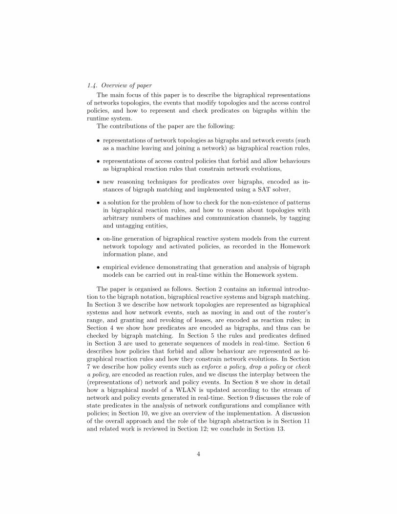
In reaction rule R3c IR′3c a pair of communication channels is establishedbetween the new machine and the machines already part of the WLAN, seeFigure 12. On the left-hand side, R3c, a node of control Properties and a node ofcontrol Properties′ specify the configurations of the new machine and a machinealready in the WLAN, respectively. On the right-hand side, R′3c, a pair of
15
Properties
Properties'
Properties
Properties
y xy x
MAC MAC
Figure 12: Reaction rule R3c IR′3c. A new machine joins the WLAN: Com-munication channels are created between the station and all the machines al-ready present in the WLAN.
communication channels is established and a node of control Properties replacesthe corresponding node of control Properties′ in R3c.
We note that initially, all machines that have already joined the WLAN aretagged, using reaction R3a IR′3a. This means the reaction is applied n times,where n is the number of machines in the network. The resulting interleavingof applications is confluent, therefore, only one sequence need be considered.Reaction R3b IR′3b is applied once. Finally, reaction R3c IR′3c is appliedn times. Again, due to confluence, only one sequence need be considered.
3.5. Revoking leases
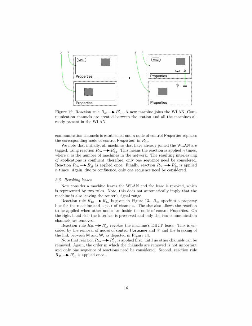
Now consider a machine leaves the WLAN and the lease is revoked, whichis represented by two rules. Note, this does not automatically imply that themachine is also leaving the router’s signal range.
Reaction rule R4a IR′4a is given in Figure 13. R4a specifies a propertybox for the machine and a pair of channels. The site also allows the reactionto be applied when other nodes are inside the node of control Properties. Onthe right-hand side the interface is preserved and only the two communicationchannels are removed.
Reaction rule R4b IR′4b revokes the machine’s DHCP lease. This is en-coded by the removal of nodes of control Hostname and IP and the breaking ofthe link between M and W, as depicted in Figure 14.
Note that reaction R4a IR′4a is applied first, until no other channels can beremoved. Again, the order in which the channels are removed is not importantand only one sequence of reactions need be considered. Second, reaction ruleR4b IR′4b is applied once.
16
Reaction rule Algebraic form
R1 IR′1
R1def= /x
(share R(x).W(y).1 ‖ idby φ
in S(x).(id | id) ‖ id1,y,x)
R′1def= /x /z /p
(share R(x).W(y).1 ‖ /y M(y, z, p).1 ‖ idby φ′
in (S(x).(id | id) | S(z) | Properties(p).MAC.1)
‖ id1,y,x,z,p)
φdef= [{1, 2}, {0}] φ′
def= [{1, 2, 3}, {1, 2}, {0}]
R2 IR′2
R2def= /x /p
(share /y M(y,x, p).1 ‖ idby φ
in (S(x).(id | id) | Properties(p).MAC.1) ‖ id1,x,p)
Figure 15: Bigraph encoding predicate “Laptop has Internet connection”.
4. Predicates
Predicates for bigraphs can be expressed in the logic BiLog [6]. However, ifwe restrict to an intensional fragment of BiLog, which omits the Boolean opera-tors and product and composition adjuncts, then any predicate can be encoded(syntactically) as a bigraph (see [4] for formal details), which can be then bechecked by reduction to bigraph matching. We have found this restriction to besuitable for the predicates we require in this application. For example predicatestypically express spatial, static properties of the systems such as “TCP traffic isblocked for machine with IP address 192.168.0.3”,“Machine 01:23:45:67:89:ab isin the range of the router’s signal”, and “Laptop has Internet connection”. Thelatter property is represented by the bigraph in Figure 15.
Definition: Let α be a predicate and Bα its bigraph encoding. Let S bea bigraph. We define S |= α iff Bα is a match in S. S 6|= α denotes Bα is not amatch in S.
We often require to reason about whether or not a machine is in the systemor part of the WLAN, especially in the context of enforcing or revoking a policy.We therefore define the following two predicates (parameterised by a machineaddress):
• ϕMAC is true iff the machine MAC is present in the system,
• ψMAC is true iff the machine MAC is part of the WLAN.
These predicates are encoded by bigraphs BϕMACand BψMAC
, depicted inFigure 16.
5. Generating models of network events in real-time
The model of the current configuration is generated and stored in the Bigraphanalysis component. Note, we generate and store the algebraic form, whereaswe use the graphical form for feedback.
19
Properties
M
W
y x
Properties
p
MACMAC
Figure 16: Bigraphs BϕMAC(left) and BψMAC
(right).
The reaction rules and predicates defined in the previous section are used togenerate sequences of models, e.g. S0, S1, . . ., from network events. For a givenmodel Sn in a sequence, we generate a successor model Sn+1 when Sn B∗ Sn+1.Strictly, any model S such that Sn B∗ S is a successor model, however, oftenwe store only the model obtained after several rewriting steps, for example whentagging and untagging is required. This means that the sequence of storedmodels corresponds exactly to the sequence of events. Generation is carried outin real-time, without interruption or delay to the network management system.
An example illustrates the generation process.Assume the Stream database generates a (derived) network event specifying
that machine A is present in the system and a DHCP lease has been granted.Let the current model be denoted by Sn, and assume the generated event hasbeen sent to the Bigraph encoder component. The sequence of reaction rules tobe applied to Sn is determined by whether or not machine A is already presentin the system and if it has joined the WLAN. Therefore, the Bigraph analysiscomponent is queried to check if Sn |= ϕA and Sn |= ψA. The results are sentback to the Bigraph encoder component. We then have three cases of modelgeneration, summarised as follows:
• If Sn |= ϕA and Sn |= ψA, then the system remains unchanged and noreaction rule is applied.
• If Sn |= ϕA but Sn 6|= ψA, then machine A has to join the WLAN. Thegenerated sequence of reactions is: R3a IR′3a, R3b IR′3b, R3c IR′3c,which is sent to the Bigraph analysis component to update the model:Sn B∗
3aB
3bB∗
3cSn+1. For brevity, we denote this sequence of ap-
plications as Sn B∗3Sn+1.
• If Sn 6|= ϕA, then machine A has to appear in the range of the routerand then to join the WLAN. The generated sequence is: R1 IR′1,R3a IR′3a, R3b IR′3b, R3c IR′3c, which is sent to the Bigraph anal-ysis component to update the model: Sn B
1B∗
3Sn+1.
Encodings for the four network events, e.g. move in and out of range, grant andrevoke leases, are summarised in Table 6.
20
Event Encoding Notation
Move in range B1
—Grant lease B∗
3aB
3bB∗
3cB∗
3Revoke lease B∗
4aB
4bB∗
4Move out range B
2—
Table 6: Encodings for network events.
Control Meaning Sort Graphical notation
Port, . . . Port number p Bold rounded boxWWW, . . . External host p Bold rounded boxP, . . . Protocol p Bold rounded boxBLOCKED All traffic forbidden p Bold rounded box
Table 7: New controls and sorts for modelling policies.
6. Bigraphical models of policies
Now we turn our attention to the representation of access control policies byreaction rules. Access control policies constrain behaviours, for example theycan constrain traffic between machines, or types of traffic. New entities aretherefore required. For example, new controls are needed to express the ban ofa given port or protocol. The additional controls are listed in Table 7, which wecall constraints. The formation rule given in Table 3 is also modified by allowingio-nodes to be linked to p-nodes.
Policies are categorised as forbid policies or allow policies. The latter arerelatively simple to represent because matching can detect the existence of aconstraint that is required to be removed. However, the representation of forbidpolicies is a little more complex.
The key idea of representing a forbid policy is to link chains of p-nodes tocommunication channels. A chain of constraints represents a conjunction ofconstraints, and several chains linked to a channel represent a disjunction ofconstraints. Some policies can be represented by a single reaction rule, whereasothers require several when a form of tagging is needed in the representation(because we consider arbitrary network topologies). We illustrate the possibleforms of representation with three example forbid policies. A summary of thereaction rules (algebraic form) for these policies is given in Table 8.
Policy 1: Consider a policy that forbids the machine named Laptop fromreceiving incoming traffic from remote host WWW, defined by the reaction rulein Figure 17. This can match only Laptop’s properties box, its out-going channelto the external world and Internet box. In the right-hand side, constraint WWWis attached to the channel’s link. Note that constraints like WWW are alwaysplaced within the sender’s bj-box. The inverse reaction P ′1 IP1 models thepolicy being dropped.
21
Properties
Internet
Properties
Internet
y c y c
Laptop
WWW
Laptop
Figure 17: Reaction rule P1 IP ′1. All incoming traffic from WWW to Laptopis blocked.
While this policy (P1) is represented by a single reaction rule, we note that itmust be applied carefully, to avoid multiple or inconsistent applications. The fol-lowing example illustrates the problem. Consider a bigraph S in which machineLaptop is already forbidden from receiving traffic from WWW, i.e. a WWW-nodeis already linked to the channel from Laptop to Internet (this is indicated by theopen link on name c in P1). The reaction rule P1 IP ′1 could be applied tothis bigraph, and as a result of the rule application, we would obtain a bigraphin which two copies of the same constraint are linked to the channel. To avoidthis, we must check, before any rule applications for the policy, whether trafficfrom WWW to Laptop is forbidden. Specifically, the Bigraph analysis compo-nent is queried to check whether S |= ϕP ′
1, where predicate ϕP ′
1corresponds to
the bigraph P ′1. The reaction rule for the policy is applied only if the predicateis false (i.e. P ′1 is not a match in S). Since the predicate holds for S, reactionrule P1 IP ′1 would not be applied in this case.
Policy 2: A more complex model arises when TCP connections with anyhost using destination ports 8080 or 6881 and source port 6882 are forbidden.First, rule P2a IP ′2a is applied once to all the channels in the system. This
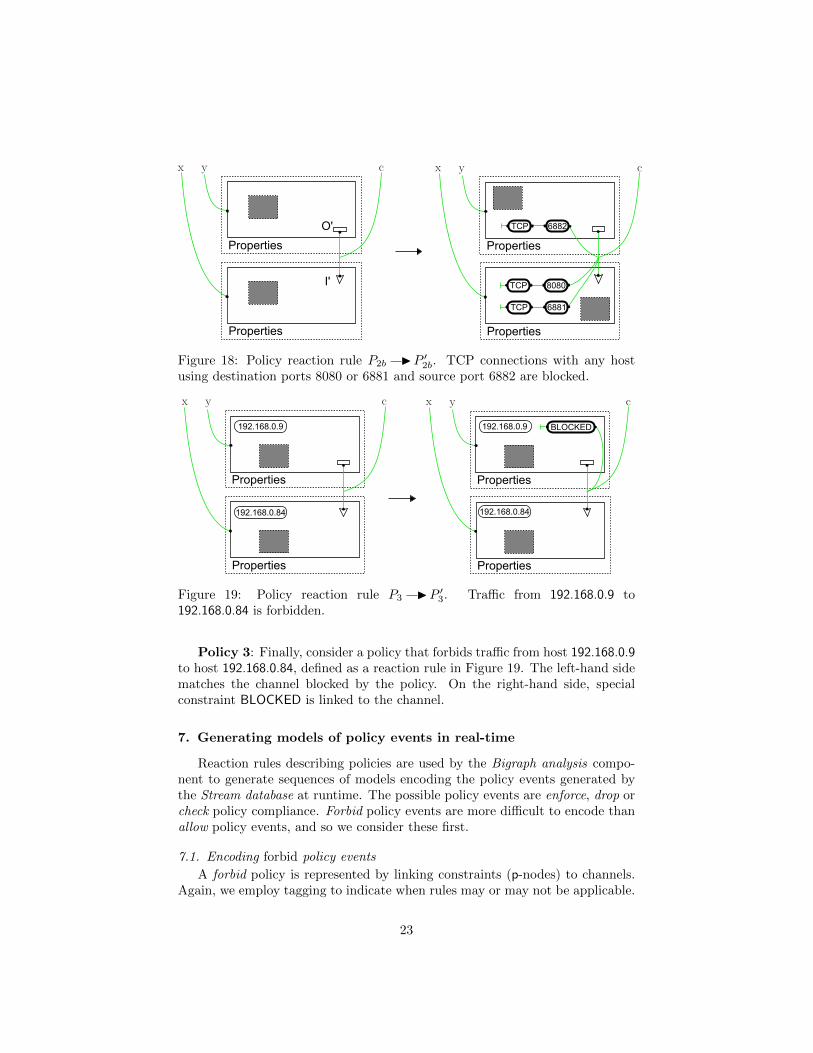
results in a bigraph in which all io-nodes are tagged, which is necessary in orderto ensure that rule P2b IP ′2b is applied only once. Second, rule P2b IP ′2b isapplied to all the tagged channels; this is depicted in Figure 18. The left-handside P2b matches any tagged channel. On the right-hand side P ′2b, the con-
straints are placed by linking them to the channels and io-nodes are untagged.Constraints on source ports are placed inside the box containing node O (i.e.sender’s Properties box), while constraints on destination ports are inside thebox containing node I (i.e. receiver’s Properties box). The order in which chan-nels are tagged and untagged is irrelevant. Thus, only one interleaving need beconsidered.
As in the previous example, the Bigraph analysis component is queried priorto the application of the reaction rules modelling this policy in order to avoiddouble entries and inconsistent constraints.
22
Properties
Properties
Properties
Properties
y cx y cx
TCP 6882
TCP 8080
TCP 6881
I'
O'
Figure 18: Policy reaction rule P2b IP ′2b. TCP connections with any hostusing destination ports 8080 or 6881 and source port 6882 are blocked.
Properties
Properties
Properties
Properties
192.168.0.9 192.168.0.9
192.168.0.84192.168.0.84
BLOCKED
y cx y cx
Figure 19: Policy reaction rule P3 IP ′3. Traffic from 192.168.0.9 to192.168.0.84 is forbidden.
Policy 3: Finally, consider a policy that forbids traffic from host 192.168.0.9to host 192.168.0.84, defined as a reaction rule in Figure 19. The left-hand sidematches the channel blocked by the policy. On the right-hand side, specialconstraint BLOCKED is linked to the channel.
7. Generating models of policy events in real-time
Reaction rules describing policies are used by the Bigraph analysis compo-nent to generate sequences of models encoding the policy events generated bythe Stream database at runtime. The possible policy events are enforce, drop orcheck policy compliance. Forbid policy events are more difficult to encode thanallow policy events, and so we consider these first.
7.1. Encoding forbid policy events
A forbid policy is represented by linking constraints (p-nodes) to channels.Again, we employ tagging to indicate when rules may or may not be applicable.
In the case of enforce, we employ tagging to ensure that constraints are onlyadded once. In the case of checking policy compliance, the use of tagging ismore subtle. The problem we need to overcome is how to check for the non-existence of a pattern in a bigraph, namely, we require to check that we cannot(bigraph) match the left hand-side of a policy enforcement rule. So, we tagchannels that comply with the policy. If all the channels are tagged, then a(bigraph) match is not possible, denoted by ���match, and we can conclude theentire model complies with the policy. Thus, for a policy P, we denote by ϕP
the predicate for compliance with policy P and BϕPthe corresponding bigraph.
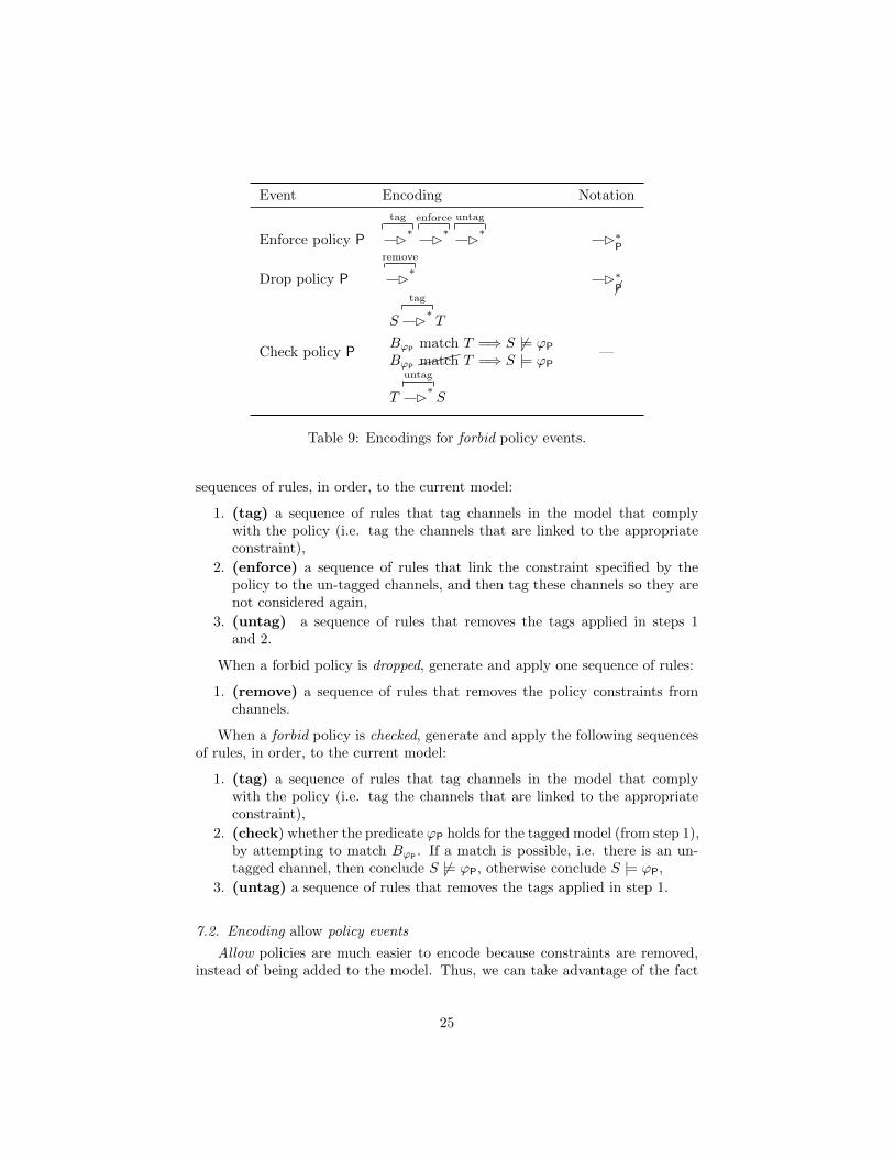
An explanation of the sequence of reaction rules that encode a forbid policyis given below, the rules are summarised in Table 9, assuming a current model S.The rules are grouped according to three functions: tag, enforce/remove/check,and untag. We note that tagging and untagging is required when enforcing orchecking a (forbid) policy because we are dealing with an arbitrary topology(with an unknown number of communication channels). Without tagging wewould be unable to determine how many channels to check. Moreover, we can’tjust match patterns of the form /c(O(c).1 ‖ I(c).1) to search for channels withoutconstraints because if such match does not exist, it does not assure us that thepolicy holds. It may not hold because the channel is linked to other constraints.
When a forbid policy is to be enforced, generate and apply the following
24
Event Encoding Notation
Enforce policy P
tag
B∗enforce
B∗
untag
B∗
B∗P
Drop policy P
remove
B∗
B∗�P
Check policy P
S
tag
B∗T
BϕPmatch T =⇒ S 6|= ϕP
BϕP ���match T =⇒ S |= ϕP
T
untag
B∗S
—
Table 9: Encodings for forbid policy events.
sequences of rules, in order, to the current model:
1. (tag) a sequence of rules that tag channels in the model that complywith the policy (i.e. tag the channels that are linked to the appropriateconstraint),
2. (enforce) a sequence of rules that link the constraint specified by thepolicy to the un-tagged channels, and then tag these channels so they arenot considered again,
3. (untag) a sequence of rules that removes the tags applied in steps 1and 2.
When a forbid policy is dropped, generate and apply one sequence of rules:
1. (remove) a sequence of rules that removes the policy constraints fromchannels.
When a forbid policy is checked, generate and apply the following sequencesof rules, in order, to the current model:
1. (tag) a sequence of rules that tag channels in the model that complywith the policy (i.e. tag the channels that are linked to the appropriateconstraint),
2. (check) whether the predicate ϕP holds for the tagged model (from step 1),by attempting to match BϕP
. If a match is possible, i.e. there is an un-tagged channel, then conclude S 6|= ϕP, otherwise conclude S |= ϕP,
3. (untag) a sequence of rules that removes the tags applied in step 1.
7.2. Encoding allow policy events
Allow policies are much easier to encode because constraints are removed,instead of being added to the model. Thus, we can take advantage of the fact
25
Event Encoding Notation
Enforce policy P
enforce
B∗
B∗P
Check policy PBϕP
match S =⇒ S 6|= ϕP
BϕP ���match S =⇒ S |= ϕP—
Table 10: Encodings for allow policy events.
that bigraph matching tests for the existence of a pattern. An overview of allowpolicy enforce/check is the following, which is also summarised in Table 10.Again, assume current model S.
When an allow policy is to be enforced, simply generate and apply a sequenceof rules that enforce the policy by removing the relevant constraints. There isno need for tagging.
When an allow policy is checked, simply attempt to match BϕP. Again, if
a match is possible, then conclude S 6|= ϕP, otherwise conclude S |= ϕP.We note that is not possible to drop an allow policy. If the user wishes to
block some behaviour, it has to be specified explicitly as a forbid policy.
7.3. Interplay between network and policy events
When a network event occurs, the Bigraph analysis component applies a se-quence of reaction rules as described in Section 5. However, this may lead to asystem in which some policies are not enforced. For example, assume a currentmodel, Sn, of a WLAN where every machine is forbidden to receive data from re-mote host WWW. Further, assume a new machine joins the WLAN. As a result,the Bigraph analysis component updates Sn to Sn+1 thus: Sn B
1B∗
3Sn+1.
But in model Sn+1, the new machine is not forbidden from receiving data fromWWW, thus the policy has to be re-enforced.
Let us call a policy that has been enforced, but not dropped, an active policy.In general, in the bigraph model, active policies need to be checked/enforced/dropped(by the Bigraph analysis component) before and/or after network and policyevents. The exact sequence depends on the event. Informally, consider eachpossible event and the requirements to check/enforce/drop active policies:
1. grant a lease - enforce active policies after granting a lease, then checkall active polices
2. revoke a lease - drop active policies before revoking a lease, enforce allactive polices afterwards, then check all active policies
3. move into signal range - check active policies after moving into signalrange
4. move out of signal range - check active policies after moving out of signalrange
5. enforce a policy - enforce new policy, and add new policy to active set,then check all active policies
26
6. drop a policy - drop the policy and remove from active set, then checkall active policies.
We can make this more precise as follows, referring to network and policyevents by the abbreviations above. For policy φ, set of active policies Φ, andsequence of network and policy events S, we define the expansion of a sequenceof events according to the function [| |] as follows:
1. [| grant; S |] Φ = grant; enforce Φ; check Φ; ([| S |] Φ)
2. [| revoke; S |] Φ = drop Φ; revoke; enforce Φ; check Φ; ([| S |] Φ)
3. [| in; S |] Φ = in; check Φ; ([| S |] Φ)
4. [| out; S |] Φ = out; check Φ; ([| S |] Φ)
5. [| enforce φ; S |] Φ = enforce φ; check {φ} ∪ Φ; ([| S |] ({φ} ∪ Φ))
6. [| drop φ; S |] Φ = drop φ; check Φ \ {φ}; ([| S |] (Φ \ {φ}))
We illustrate the process, in detail, in the next section.
8. Example of interplay between network events and policy events inreal-time
We show step-by-step how updates are made to the current bigraphicalmodel of the WLAN, according to the events from the Stream database. Weindicate sequences of WLAN models by S0, S1, . . .. Due to confluence proper-ties, we consider only one possible sequence of updates.
Initially, no stations are present, as given by bigraph S0 in Figure 7. Nowconsider the following scenario, a summary of which is given in Table 11.
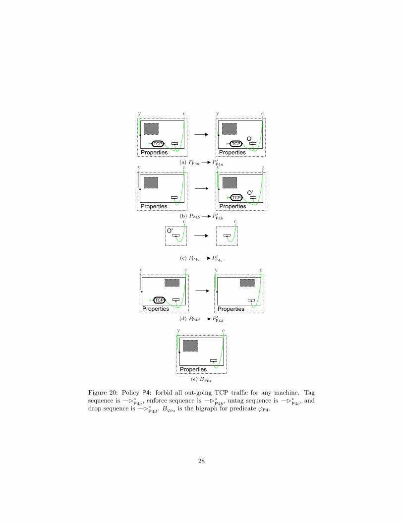
1. The user specifies and enforces a new policy that all out-going TCP trafficfor any machine is forbidden. This user-action generates a policy event, whichtriggers the generation of the reaction rules for a forbid policy. We denote thepolicy by P4 and give the reaction rules in Figure 20. A brief explanation of therules is the following. Reaction rule PP4a IP ′P4a tags any out-going channelof any machine that is part of the WLAN3 and complies with P4. Reaction rulePP4b IP ′P4b matches any untagged channel and thus it enforces the policy.On the right hand-side, P ′P4b, a TCP-node is linked to the matched channel andthe channel is tagged (to avoid further treatment). Untagging reaction rulePP4c IP ′P4c removes the tags. Bigraph BϕP4
matches any untagged out-goingchannel and as described in Section 7, P4 is violated when BϕP4
is a matchin the temporary state in which all blocked out-going channels are tagged. Atthis point, the Bigraph analysis component enforces P4 on S0 and we haveS0 B∗
P4S0, i.e. no reaction rule is applicable because no machines are present
in S0. Policy P4 is also checked. Since BϕP4is not a match, P4 holds.
2. Machine MAC1 enters a location covered by the router’s signal. SinceS0 6|= ϕMAC1, the Bigraph encoder component instantiates4 reaction ruleR1 IR′1
3A channel is present thus a DHCP lease has already been granted.4Special control MAC is replaced by actual address MAC1.
27
Properties
y c
TCPO'
Properties
y c
TCP
(a) PP4a IP ′P4a
Properties
y c
Properties
y c
TCPO'
(b) PP4b IP ′P4bc
O'
c
(c) PP4c IP ′P4c
Properties
y c
Properties
y c
TCP
(d) PP4d IP ′P4d
Properties
y c
(e) BϕP4
Figure 20: Policy P4: forbid all out-going TCP traffic for any machine. Tagsequence is B∗
P4a, enforce sequence is B∗
P4b, untag sequence is B∗
P4c, and
drop sequence is B∗P4d
. BϕP4is the bigraph for predicate ϕP4.
28
Properties
S
M
RW
Internet
SMAC1
Properties
S
M
RW
Internet
SMAC1
IP1
N1
Properties
S
M
RW
Internet
SMAC1
IP1
N1
TCP
Figure 21: States S1 (upper left), S2 (upper right), S3 (lower). In State S3
MAC1 is part of the network and P4 is enforced.
and the Bigraph analysis component updates the system: S0 B1S1. After
this step, the Bigraph encoder component checks whether P4 is violated. In thiscase, reaction rule PP4a IP ′P4a is not applicable and BϕP4
is not a match inS1. Therefore, the policy is not violated.
3. A DHCP lease is granted to machine MAC1. In the current state wehave S1 |= ϕMAC1 and S1 6|= ψMAC1. Therefore, the Bigraph analysis componentupdates the system by applying instantiated rules R3a IR′3a, R3b IR′3b,and R3c IR′3c: S1 B∗
3aB
3bB∗
3cS2. After the topology update, the Bi-
graph analysis component enforces P4 in S2. The following updates are per-formed: S2 B∗
P4aB∗
P4bB∗
P4cS3
5. We indicate this sequence of rules byB∗
P4. States S1, S2 and S3 are shown in Figure 21.
4. MAC2 enters a location covered by the router’s signal. Since S3 6|=ϕMAC2, the Bigraph analysis component performs the same sequence describedin step 2 above when machine MAC1 entered the signal range. Specifically, first,the topology is updated with S3 B
1S4. Second, P4 is enforced by the usual
tagging, matching, untagging sequence: S4 B∗P4S4. Observe that no update
is performed because reaction rule PP4b IP ′P4b is not applicable (there are no
5In this case B∗ is B because only one machine is part of the network in S2.
29
Properties
SS
M
RW
Internet
S
M
Properties
MAC2
MAC1 IP1 N1
TCP
Figure 22: State S4: MAC2 enters the router’s signal range, MAC1 is part of theWLAN and P4 is enforced.
Properties
SS
M
RW
Internet
S
M
Properties
MAC2
MAC1 IP1 N1
TCP
IP2 N2
TCP
TCP
TCP
Figure 23: State S5: MAC1 and MAC2 joined the WLAN and P4 is enforced.
out-going channels requiring to be blocked in machine MAC2). Finally ϕP4 ischecked. Since BϕP4
is not a match in T4, P4 is not violated. The bigraph forupdated model S4 is given in Figure 22.
5. A DHCP lease is granted to machine MAC2. The status of the configu-ration is S4 |= ϕMAC2 and S4 6|= ψMAC2. Hence, the Bigraph analysis componentupdates the model by applying the sequence of reaction rules encoding a joinevent: S4 B∗
3S′4. Then, the policy is enforced with S′4 B∗
P4S5. Finally, the
Bigraph analysis component checks whether ϕP4 holds. Since BϕP4does not
occur in T5, we have S5 |= ϕP4. The bigraph for S5 is given in Figure 23.The sequence of events and the corresponding model updates described are
summarised in Table 11.
9. Bigraph model analysis
At any point in the model generation process we can check whether thebigraphical representation of the current system satisfies compliance with a pol-icy, or an invariant, or indeed any property that can be defined in the fragment
30
Event Updates WLAN model Policy
1. P4 enforced
S0 B∗P4S0
S0 B∗P4a
T0BϕP4 ���match T0T0 B∗
P4cS0
check P4S0 S0 |= ϕP4
2. MAC1 in sig-nal range
S0 6|= ϕMAC1
S0 B1S1 B∗
P4S1
S1 B∗P4a
T1BϕP4 ���match T1T1 B∗
P4cS1
check P4S1 S1 |= ϕP4
3. MAC1 leasegranted
S1 |= ϕMAC1 and S1 6|= ψMAC1
S1 B∗3S2 B∗
P4S3
S3 B∗P4a
T3BϕP4 ���match T3T3 B∗
P4cS3
check P4S3 S3 |= ϕP4
4. MAC2 in sig-nal range
S3 6|= ϕMAC2
S3 B1
B∗P4S4
S4 B∗P4a
T4BϕP4 ���match T4T4 B∗
P4cS4
check P4S4 S4 |= ϕP4
5. MAC2 leasegranted
S4 |= ϕMAC2 and S4 6|= ψMAC2
S4 B∗3
B∗P4S5
S5 B∗P4a
T5BϕP4 ���match T5T5 B∗
P4cS5
check P4S5 S5 |= ϕP4
Table 11: Generation of models S0 B · · · BS5.
of BiLog. For example, we check invariants after every update of the system,logging any violations and reporting them, as required, to the system and/oruser. We can also detect conflicting policies, as follows. We assume the right-hand side of reaction rules for policies as invariants. A new policy conflicts withan existing one whenever its application invalidates an invariant. As a simpleexample, consider reaction rule P1 BP ′1 and its inverse P ′1 BP1 introducedin Section 6. Assume that Laptop is the only machine in the system and noconstraints are in place. Call the bigraph representing this state Sn. When thesystem is updated by P1 BP ′1, right-hand side P ′1 is adopted as an invariant.The evolution of the system is given by Sn B
1Sn+1. Now consider an appli-
cation of the inverse rule, so the system evolves: Sn+1 B1′Sn+2 = Sn. At
this point the invariant is checked. Since P ′1 is not a match in Sn+2 (node ofcontrol WWW cannot be matched), then Sn+2 6|= P ′1, thus indicating a conflictbetween the two policies. This is a simple example: a policy and its inverse aretrivially in conflict and in this case the policies are implemented by single rules.
31
S0 BS1 B · · · BSn
B· · ·
B · · ·B · · ·&%
'$Transition system
Figure 24: Generating all possible evolutions from current state Sn.
In general, checking for conflicts will be more complicated because a policy isimplemented by a sequence of reactions (e.g. because of tagging/untagging). Inany event, the run-time system can either indicate this to the user, deny theenforcement of the second policy, or just keep track of conflicts in a logfile.
It is possible to reason about the evolution of the system with temporal prop-erties such as “Eventually machine 01:23:45:67:89:ab will be connected to Lap-top”, “TCP traffic is always blocked for machine with IP address 192.168.0.3”,“A lease is granted to machine 01:23:45:67:89:ab until it is not in the range ofthe router’s signal”. These properties can be expressed in an appropriate (e.g.linear or branching time) temporal logic and then checked in a transition systemof all possible evolutions, generated from the current state. See Figure 24 for anillustration. In order to generate a finite structure, a fixed set of machines andpolicies would have to be specified. Further, to reflect likely user behaviours,allowable events have to be specified (otherwise, from any state we could returnto S0). For example, we might wish to reason about future behaviour, basedon the assumption that no machines leave the network, or no new policies areenforced.
Given a finite transition system, checking a temporal property involves bi-graph matching for state formulae and standard model checking techniques forthe temporal operators. The latter is computationally expensive and may notbe tractable in real-time, depending on the number of machines and policies andon the temporal formula. So far, we have not found a need for temporal prop-erties: state formulae are currently sufficient for all verification needs expressedby the Homework system users.
10. Implementation
A prototype system is fully implemented on the Homework router, whichis hosted on a variety of small form-factor PCs. The bigraph generation isimplemented in OCaml; the matching engine is based on the MiniSat solver [7]and is written in C++. The Bigraph encoder and Bigraph analysis componentsare part of the more extensive BigraphER (Bigraph Evaluator and Rewriting)System [8]. The software runs on a standard Linux Ubuntu distribution. Accesscontrol is enforced via NOX (which implements the custom DHCP server) andOpen vSwitch, as dictated by the Ponder2 policy engine [9], based on eventsrecorded in the Homework database.
32
00.010.020.030.040.050.060.070.080.09
0.1
302520151051
Ave
rage
upd
ate
time
(s)
Machines
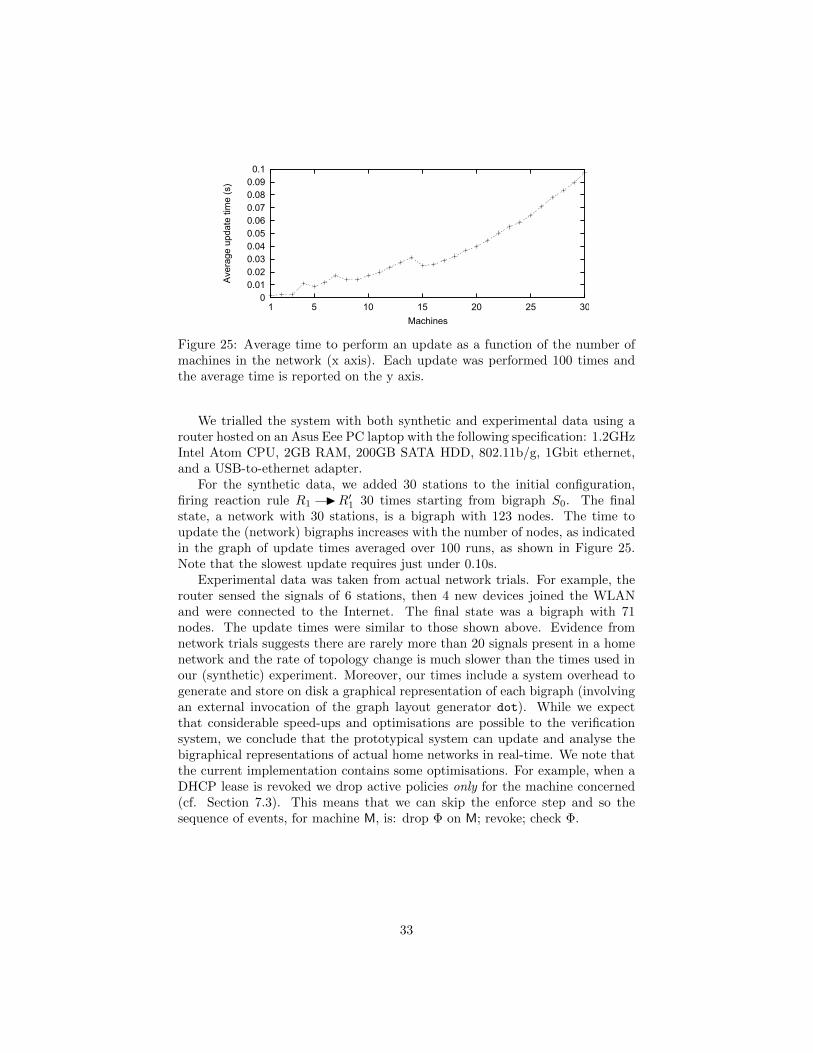
Figure 25: Average time to perform an update as a function of the number ofmachines in the network (x axis). Each update was performed 100 times andthe average time is reported on the y axis.
We trialled the system with both synthetic and experimental data using arouter hosted on an Asus Eee PC laptop with the following specification: 1.2GHzIntel Atom CPU, 2GB RAM, 200GB SATA HDD, 802.11b/g, 1Gbit ethernet,and a USB-to-ethernet adapter.
For the synthetic data, we added 30 stations to the initial configuration,firing reaction rule R1 IR′1 30 times starting from bigraph S0. The finalstate, a network with 30 stations, is a bigraph with 123 nodes. The time toupdate the (network) bigraphs increases with the number of nodes, as indicatedin the graph of update times averaged over 100 runs, as shown in Figure 25.Note that the slowest update requires just under 0.10s.
Experimental data was taken from actual network trials. For example, therouter sensed the signals of 6 stations, then 4 new devices joined the WLANand were connected to the Internet. The final state was a bigraph with 71nodes. The update times were similar to those shown above. Evidence fromnetwork trials suggests there are rarely more than 20 signals present in a homenetwork and the rate of topology change is much slower than the times used inour (synthetic) experiment. Moreover, our times include a system overhead togenerate and store on disk a graphical representation of each bigraph (involvingan external invocation of the graph layout generator dot). While we expectthat considerable speed-ups and optimisations are possible to the verificationsystem, we conclude that the prototypical system can update and analyse thebigraphical representations of actual home networks in real-time. We note thatthe current implementation contains some optimisations. For example, when aDHCP lease is revoked we drop active policies only for the machine concerned(cf. Section 7.3). This means that we can skip the enforce step and so thesequence of events, for machine M, is: drop Φ on M; revoke; check Φ.
33
11. Discussion
In this section we give an overview of modelling and design decisions we havemade and the implications for our overall approach.
11.1. Why model with BRS?
Our models are one of the first applications of BRS to a real world problemand modelling the management of wireless networks with BRS has some advan-tages over other process calculi. Arguably the most important advantage is theability to express spatial aspects of computation in a natural, hierarchical way,a feature lacking in formalisms such as the π-calculus and CCS where the un-derlying spatial structure is assumed to be flat. Cardelli and Gordon’s calculusof mobile ambients [10] is closer to BRS and allows the location hierarchy to beorganised into a tree structure. Additionally, this structure can be representedgraphically by using boxes to encode locations and the nesting of boxes to en-code their topology. However, computation is encoded solely by changes in thespatial structure. In BRS, computation can also be encoded by changes in thelink graph structure. While these process calculi are fundamentally equivalent,bigraphs allow for an easier representation of complex systems by keeping theconcepts of space and computation separated. In contrast, as a consequence ofthe structural operational semantics of process calculi, non-trivial protocols arerequired when encoding complex state modifications.
Nevertheless we did encounter one drawback with BRS modelling, whicharises from the declarative nature of reaction rules (and suffered by all processcalculi). Recall, we employed tagging in our reaction rules to overcome problemsin three scenarios:
1. the requirement to apply a rule n times, because we have arbitrary topolo-gies,
2. the requirement to ensure that we do not duplicate the application of arule,
3. the requirement to encode universal quantification (e.g. there does notexist a non-match for a given predicate).
Essentially, these problems are a consequence of the declarative nature of rewriterules and rewriting: in these scenarios we require a notion of control. We could,for example, define that control explicitly, with a reaction rule for each valueof n. But this is rather clumsy and would obscure the clarity of the model;it also assumes we can define a static upper bound. A better solution wouldbe to introduce parameterised reaction rules into BRS, as syntactic sugar, thusavoiding the need for tagging. This is future work.
11.2. Do we have the right abstraction?
We currently model exactly what the router senses and the subsequent eventsstored in the Stream database. But we could add additional features such as thephysical location of devices, or ownership of machines, if they can constrain
34
behaviour. Moreover we could also add aspects of real-time, such as the rateof events or timed policies (e.g. a policy applies between 18:00 and 24:00 everyday, or on a given day), if these become relevant. More generally, we aim tomodel the events recognised and stored by the Homework network managementsystem; if the system monitors more detailed behaviour, then the abstractionand the subsequent formal models must reflect that.
11.3. Do we have the abstraction right?
In other words, are our models faithful to the actual system, do they abstractfrom the same semantics? This is a problem for any modelling approach. Inthe case of network events, it is fairly straightforward to see our abstraction isfaithful. In the case of the policies, there are often subtleties about how exactlyto interpret a policy, which may depend on user intentions. We have presentedpolicy enforcement and dropping in detail deliberately, so as to expose thesesubtleties and why and how user comprehension and implementation can bedifficult. Throughout the project we have discussed policy design and imple-mentation with the developers of the policy engine, using the bigraph graphicalnotation. This has provided informal validation that bigraph models can helppolicy language designers agree on interpretations and resolve ambiguity.
11.4. Can we use the sequence of models in other ways?
The approach we have described here is a form of runtime verification, inthat we construct a directed simulation and test for behaviors satisfying orviolating certain properties. Our approach is not based on data traces or dead-lock detection, rather it is a form of runtime formal modelling. While this hassignificant overheads, compared to more conventional runtime verification, wepropose that the additional requirements of behaviour that is both spatial aswell as temporal, can justify this. The result is much richer feedback that in-forms the user’s cognitive model. For example, traditional verification mightreport that a packet was observed on a channel, or a variable has a particularvalue, whereas we can report a much more detailed model (of the state of thesystem) that explains current spatial relationships and communication links.We could make further use of the sequence of generated models, for examplefor debugging and for supporting understanding the causes of failure (e.g. wecould rollback and replay), or for generating tests from the results of the failedverifications.
11.5. Can we improve feedback?
As we have stated earlier, our long-term motivation is to aid users in theirunderstanding of the state of their system, and to give feedback to developersabout user experiences. We have not yet carried out a formal evaluation of this,but informal evaluations from the (Homework) system developers is that thebigraphical feedback from the runtime verification is helpful to them. However,while bigraphs permit a straightforward and intuitive graphical representation,
35
we conjecture that our system representations, which are based on Venn dia-grams, may be too unfamiliar and/or detailed for non-expert users. We planto experiment with other graphical representations that can be generated au-tomatically from our bigraphs. For example, can we generate the cartoon inFigure 2 from the bigraph in Figure 3; can we generate the cartoons used in theHomework system drag and drop interface for policies? Are there constraintson the style of cartoons that can be generated from our bigraphs? Furthermore,we may not wish to reveal all the detail initially, but, for example, only presentproperties when the user rolls a mouse over the (representation of) a machine.This will be future work.
12. Related work
There is a significant body of work on analysis of policies and conflicts inthe context of network management, for example [11], but we are unaware ofany approach involving real-time analysis of process calculi models.
Runtime models for managing the complexity of evolving software behaviourwhile it is executing is a recent area of interest, particularly in the domain of self-adaptation (e.g. recent Dagstuhl seminar [12]). While our domain is different,our work has a similar goal in that it is reasoning about context-dependenciesat runtime. We note a related online, event-driven formal modelling approachtaken in [13] to checking configurations of a home-care application. In this case,the configuration data was streamed from log files of user activity; empirical useof the reasoning system also revealed state-based reasoning was sufficient andthere was no need for temporal operators.
13. Conclusions
We have extended the Homework network management system with runtimeverification comprising real-time generation and analysis of bigraphical modelsof network topology, network events and access policies. This work representsone of the first applications of bigraphical modelling to a real world problem,and a novel use of process algebraic modelling in a runtime verification context.
Both standard network events, such as a machine entering a signal range orhaving a DHCP lease revoked, and forbid and allow access policy enforcement ordropping, are represented by bigraph reaction rules. We have presented the fulldetails of the representation so as to expose the precise details of how policieswork and their interplay with network events.
Many rules involve the concept of “tagging” entities, to limit the scope ofapplicability of the rules. While this adds some complexity to the representation,it is an inevitable consequence of reasoning about complex computation withdeclarative rules.
The real-time generation of bigraph models is event-driven: we apply thereaction rules of a bigraphical reactive system, according to events captured inthe Homework stream database. In essence, we generate a real-time simulation
36
trace, where states are bigraph representations of the live system: at each step,the bigraph state is checked for invariants and violations are reported to theuser.
Verification is done via a bespoke software component, based on reasoningabout predicates by bigraph matching, encoded in a SAT solver. The verificationsystem is fully implemented on the router and our experiments indicate thatmodel generation and analysis can be carried out in real-time. We have outlinedhow to model-check temporal properties, but so far there is little evidence fromuser trials that temporal operators are required.
Future work will be in three areas: feedback, efficiency, and quantitive be-haviour. The first includes developing and evaluating different forms and typeof feedback about the outcomes of the verification process to both the user andthe system. For example, we will extend the system so that the Bigraph anal-ysis component communicates directly with the Stream database component.Whenever an invariant is not satisfied, the violation is recorded in a table inthe database; users and diagnostic applications can subscribe to the table andobtain real-time updates of the system status. We will also explore (graphical)abstractions of bigraphical representations that may be more accessible and/ormeaningful to users, and conduct user trials with them. We will consider extend-ing the matching engine in the Bigraph encoder component to support regularexpressions on controls. This can greatly reduce the number of matching in-stances, especially when reaction rules involve ranges of addresses. Finally, wewill extend the modelling to stochastic bigraphs [14], to represent the rate oftraffic and bandwidth capabilities, thus extending the range of policies we canconsider.
Acknowledgments
This work is supported by the Homework Research Project, funded by theEngineering and Physical Sciences Research Council, under grant EP/F064225/1.
References
[1] J. Sventek, A. Koliousis, O. Sharma, N. Dulay, D. Pediaditakis, M. Sloman,T. Rodden, T. Lodge, B. Bedwell, K. Glover, An Information Plane Archi-tecture Supporting Home Network Management, Proceedings of the 12thIFIP/IEEE International Symposium on Integrated Network Management(2011) 1–8.
[2] R. Mortier, B. Bedwell, K. Glover, T. Lodge, T. Rodden, C. Rotsos, A. W.Moore, A. Koliousis, J. Sventek, Supporting novel home network manage-ment interfaces with openflow and nox, SIGCOMM Comput. Commun.Rev. 41 (4) (2011) 464–465. doi:10.1145/2043164.2018523.
[3] R. Milner, The space and motion of communicating agents, CambridgeUniversity Press, 2009.
37
[4] M. Sevegnani, Bigraphs with sharing and applications in wireless networks,PhD thesis, University of Glasgow (2012).
[5] L. Birkedal, T. C. Damgaard, A. J. Glenstrup, R. Milner, Matching of bi-graphs, Electronic Notes in Theoretical Computer Science 175 (4) (2007) 3– 19, Proceedings of the Workshop on Graph Transformation for Concur-rency and Verification (GT-VC 2006). doi:10.1016/j.entcs.2007.04.013.
[6] G. Conforti, D. Macedonio, V. Sassone, Spatial logics for bigraphs, in:L. Caires, G. Italiano, L. Monteiro, C. Palamidessi, M. Yung (Eds.), Au-tomata, Languages and Programming, Vol. 3580 of LNCS, Springer, 2005,pp. 766–778.
[7] N. Een, N. Sorensson, An extensible SAT-solver, in: SAT 2003, LNCS vol.2919, 2003, pp. 502–518.
[8] M. Sevegnani, BigraphER.URL http://www.dcs.gla.ac.uk/∼michele/bigrapher.html
[9] K. Twidle, N. Dulay, E. Lupu, M. Sloman, Ponder2: A policy system forautonomous pervasive environments, The Fifth International Conferenceon Autonomic and Autonomous Systemsdoi:10.1109/ICAS.2009.42.
[10] L. Cardelli, A. D. Gordon, Mobile ambients, Electr. Notes Theor. Comput.Sci. 10 (1997) 198–201.
[11] A. Bandara, J. Lobo, Calo, E. S. Lupu, A. Russo, M. Sloman, Toward aFormal Characterization of Policy Specification Analysis, in: Annual Con-ference of ITA (ACITA), University of Maryland, USA, 2007.
[12] U. Aßmann, N. Bencomo, B. H. C. Cheng, R. B. France, [email protected](Dagstuhl Seminar 11481), Dagstuhl Reports 1 (11) (2012) 91–123.URL http://drops.dagstuhl.de/opus/volltexte/2012/3379
[13] M. Calder, P. Gray, C. Unsworth, Is my configuration any good: checkingusability in a sensor-based activity monitor, Innovations in Systems andSoftware Engineering (2013) in press,doi:10.1007/s11334-013-0203-1.
[14] J. Krivine, R. Milner, A. Troina, Stochastic bigraphs, Electr. Notes Theor.Comput. Sci. 218 (2008) 73–96.