Real Wage Inequality Enrico Moretti UC Berkeley, NBER, CEPR and IZA First Draft: May 2008 This Draft February 2011 Abstract. A large literature has documented a significant increase in the difference between the wage of college graduates and high school graduates over the past 30 years. I show that from 1980 to 2000, college graduates have experienced relatively larger increases in cost of living, because they have increasingly concentrated in metropolitan areas that are characterized by a high cost of housing. When I deflate nominal wages using a location-specific CPI, I find that the difference between the wage of college graduates and high school graduates is lower in real terms than in nominal terms and has grown less. At least 22% of the documented increase in college premium is accounted for by spatial differences in the cost of living. The implications of this finding for changes in well-being inequality depend on why college graduates sort into expensive cities. Using a simple general equilibrium model of the labor and housing markets, I consider two alternative explanations. First, it is possible that the relative supply of college graduates increases in expensive cities because college graduates are increasingly attracted by amenities located in those cities. In this case, the higher cost of housing reflects consumption of desirable local amenities, and there may still be a significant increase in well-being inequality even if the increase in real wage inequality is limited. Alternatively, it is possible that the relative demand for college graduates increases in expensive cities due to shifts in the relative productivity of skilled labor. In this case, the relative increase in skilled workers’ standard of living is offset by the higher cost of living. The evidence indicates that changes in the geographical location of different skill groups are mostly driven by changes in their relative demand. I conclude that the increase in well-being disparities between 1980 and 2000 is smaller than previously thought. I thank David Autor, Dan Black, David Card, Tom Davidoff, Ed Glaeser, Chang-Tai Hsieh, Matt Kahn, Pat Kline, Douglas Krupka, David Levine, Adam Looney and Krishna Pendakur for insight- ful conversations, and seminar participants at Banco de Portugal, Berkeley Economics, Berkeley Haas, Bocconi, Bologna, British Columbia, Chicago Harris, Collegio Carlo Alberto, Edinburgh, Federal Reserve Board of Governors, IZA, Milano, Missouri, NBER Summer Institute, Northwest- ern, Oxford, San Francisco Federal Reserve, Simon Fraser, Stanford, Stanford GSB, UCLA, UC Santa Cruz, Toronto, Tulane, UC Merced, Verona and Victoria for many useful comments. I thank Emek Basker for generously providing the Accra data on consumption prices. Issi Romen, Mariana Carrera, Justin Gallagher, Jonas Hjort, Max Kasy and Zach Liscow provided excellent research assistance.
Transcript
Real Wage Inequality
Enrico MorettiUC Berkeley, NBER, CEPR and IZA
First Draft: May 2008This Draft February 2011
Abstract. A large literature has documented a significant increase in the difference betweenthe wage of college graduates and high school graduates over the past 30 years. I show that from1980 to 2000, college graduates have experienced relatively larger increases in cost of living, becausethey have increasingly concentrated in metropolitan areas that are characterized by a high cost ofhousing. When I deflate nominal wages using a location-specific CPI, I find that the differencebetween the wage of college graduates and high school graduates is lower in real terms than innominal terms and has grown less. At least 22% of the documented increase in college premiumis accounted for by spatial differences in the cost of living. The implications of this finding forchanges in well-being inequality depend on why college graduates sort into expensive cities. Usinga simple general equilibrium model of the labor and housing markets, I consider two alternativeexplanations. First, it is possible that the relative supply of college graduates increases in expensivecities because college graduates are increasingly attracted by amenities located in those cities. Inthis case, the higher cost of housing reflects consumption of desirable local amenities, and theremay still be a significant increase in well-being inequality even if the increase in real wage inequalityis limited. Alternatively, it is possible that the relative demand for college graduates increases inexpensive cities due to shifts in the relative productivity of skilled labor. In this case, the relativeincrease in skilled workers’ standard of living is offset by the higher cost of living. The evidenceindicates that changes in the geographical location of different skill groups are mostly driven bychanges in their relative demand. I conclude that the increase in well-being disparities between1980 and 2000 is smaller than previously thought.
I thank David Autor, Dan Black, David Card, Tom Davidoff, Ed Glaeser, Chang-Tai Hsieh, MattKahn, Pat Kline, Douglas Krupka, David Levine, Adam Looney and Krishna Pendakur for insight-ful conversations, and seminar participants at Banco de Portugal, Berkeley Economics, BerkeleyHaas, Bocconi, Bologna, British Columbia, Chicago Harris, Collegio Carlo Alberto, Edinburgh,Federal Reserve Board of Governors, IZA, Milano, Missouri, NBER Summer Institute, Northwest-ern, Oxford, San Francisco Federal Reserve, Simon Fraser, Stanford, Stanford GSB, UCLA, UCSanta Cruz, Toronto, Tulane, UC Merced, Verona and Victoria for many useful comments. I thankEmek Basker for generously providing the Accra data on consumption prices. Issi Romen, MarianaCarrera, Justin Gallagher, Jonas Hjort, Max Kasy and Zach Liscow provided excellent researchassistance.
1 Introduction
One of the most important developments in the US labor market over the past 30 years
has been a significant increase in wage inequality. For example, the difference between the
wage of skilled and unskilled workers has increased significantly since 1980. The existing
literature has focused on three classes of explanations: an increase in the relative demand
for skills caused, for example, by skill biased technical change; a slowdown in the growth
of the relative supply of skilled workers; and the erosion of labor market institutions that
protect low-wage workers.1
In this paper, I re-examine how inequality is measured and how it is interpreted. I
begin by noting that skilled and unskilled workers are not distributed uniformly across cities
within the US, and I assess how existing estimates of inequality change when differences in
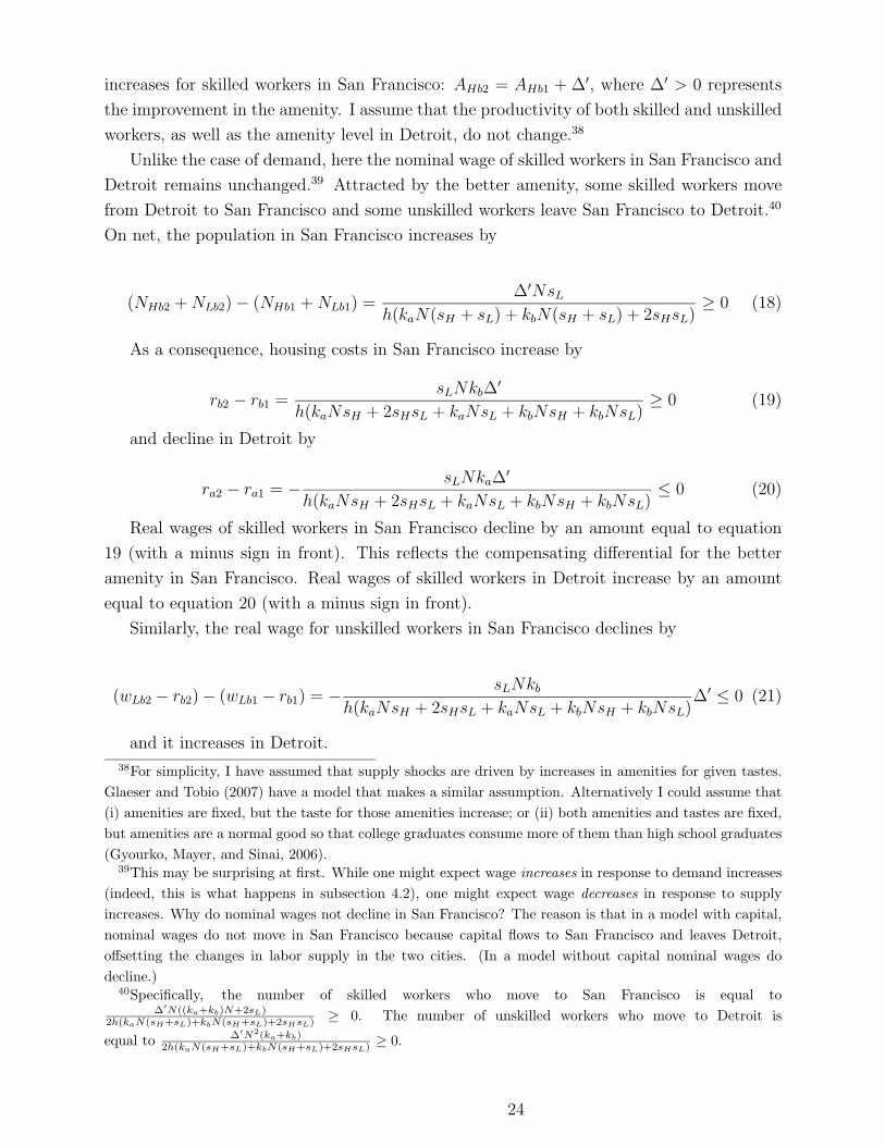
the cost of living across locations are taken into account. I then discuss how to interpret
these measures of real wage inequality when changes in amenities are different across cities.
I focus on changes between 1980 and 2000 in the difference in the average hourly wage for
workers with a high school degree and workers with college or more. Using Census data, I
show that from 1980 to 2000 college graduates have increasingly concentrated in metropolitan
areas with a high cost of housing. This is due both to the fact that college graduates in 1980
are overrepresented in cities that experience large increases in housing costs and to the fact
that much of the growth in the number of college graduates has occurred in cities with initial
high housing costs. College graduates are therefore increasingly exposed to a high cost of
living and the relative increase in their real wage may be smaller than the relative increase
in their nominal wage.
To measure the wage difference between college graduates and high school graduates
in real terms, I deflate nominal wages using a cost of living index that allows for price
differences across metropolitan areas. I closely follow the methodology that the Bureau
of Labor Statistics uses to build the official CPI, while allowing for changes in the cost of
housing to vary across metropolitan areas. Since housing is by far the largest item in the
CPI—accounting for more than a third of the index—geographical differences in housing
costs have the potential to significantly affect the local CPI. In some specifications, I also
allow for local variation in non-housing prices.
The results are striking. First, I find that between 1980 and 2000, the cost of housing
for college graduates grows much faster than cost of housing for high school graduates.
Specifically, in 1980 the difference in the average cost of housing between college and high
school graduates is only 4%. This difference grows to 14% in 2000, or more than three times
the 1980 difference. Second, consistent with what is documented by the previous literature,
I find that the difference between the nominal wage of high school and college graduates has
increased 20 percentage points between 1980 and 2000. However, the difference between the
real wage of high school and college graduates has increased significantly less. Changes in the
1A comprehensive survey is found in Katz and Autor (1999).
1
cost of living experienced by high school and college graduates account for about a quarter
of the increase in the nominal college premium over the 1980-2000 period. This finding does
not appear to be driven by different trends in relative worker ability or housing quality and
is robust to a number of alternative specifications. Third, the difference between the wage of
college graduates and high school graduates is smaller in real terms than in nominal terms
for each year. For example, in 2000 the difference is 60% in nominal terms and 51% in real
terms.
Overall, the difference in the real wage between skilled and unskilled workers is smaller
than the nominal difference and has grown less.2 Does this finding mean that the significant
increases in wage disparities that have been documented by the previous literature over the
last 30 years have failed to translate into significant increases in disparities in well-being?
Not necessarily. Since local amenities differ significantly across cities, changes in real wages
do not necessarily equal changes in well-being.
To understand the implications of my empirical findings for well-being inequality, I use a
simple general equilibrium model of the housing and labor markets with two types of labor,
skilled and unskilled.3 The model indicates that the implications of my empirical findings for
well-being inequality crucially depend on why college graduates tend to sort into expensive
metropolitan areas. I consider two possible explanations. First, it is possible that college
graduates move to expensive cities because firms in those cities experience an increase in
the relative demand for skilled workers. This increase can be due to localized skill-biased
technical change or positive shocks to the product demand for skill intensive industries
that are predominantly located in expensive cities (for example, high tech and finance are
mostly located in expensive coastal cities). If college graduates increasingly concentrate in
expensive cities such as San Francisco and New York because the jobs for college graduates
are increasingly concentrated in those cities—and not because they particularly like living
in San Francisco and New York—then the increase in their utility level is smaller than the
increase in their nominal wage. In this scenario, the increase in well-being inequality is
smaller than the increase in nominal wage inequality because of the higher costs of living
faced by college graduates.
Alternatively, it is possible that college graduates move to expensive cities because the
relative supply of skilled workers increases in those cities. This may be due, for example, to
an increase in the local amenities that attract college graduates. In this scenario, increases in
the cost of living in these cities reflect the increased attractiveness of the cities and represent
the price to pay for the consumption of desirable amenities. This consumption arguably
2It is worth stressing that changes in cost of living, while clearly important, account only for a fraction
of the overall increase in wage inequality in this period.3The model clarifies what happens to employment, wages, costs of housing of skilled and unskilled workers
and when a local economy experiences a shock to the productivity of skilled labor or a change in local
amenities. Unlike Roback (1982), productivity and amenity shocks are not necessarily fully capitalized into
land prices. This allows shocks to the relative demand and relative supply of skilled workers in a city to have
different effects on the well-being of skilled and unskilled workers and landowners.
2
generates utility. If college graduates move to expensive cities like San Francisco and New
York because they want to enjoy the local amenities—and not primarily because of labor
demand—then there may still be a significant increase in utility inequality even if the increase
in real wage inequality is limited.4 Of course, the two scenarios are not mutually exclusive,
since in practice it is possible that both relative demand and supply shift at the same time.
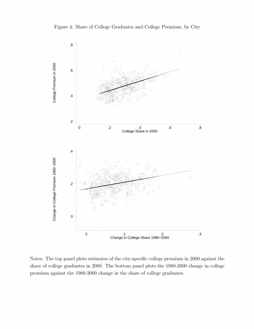
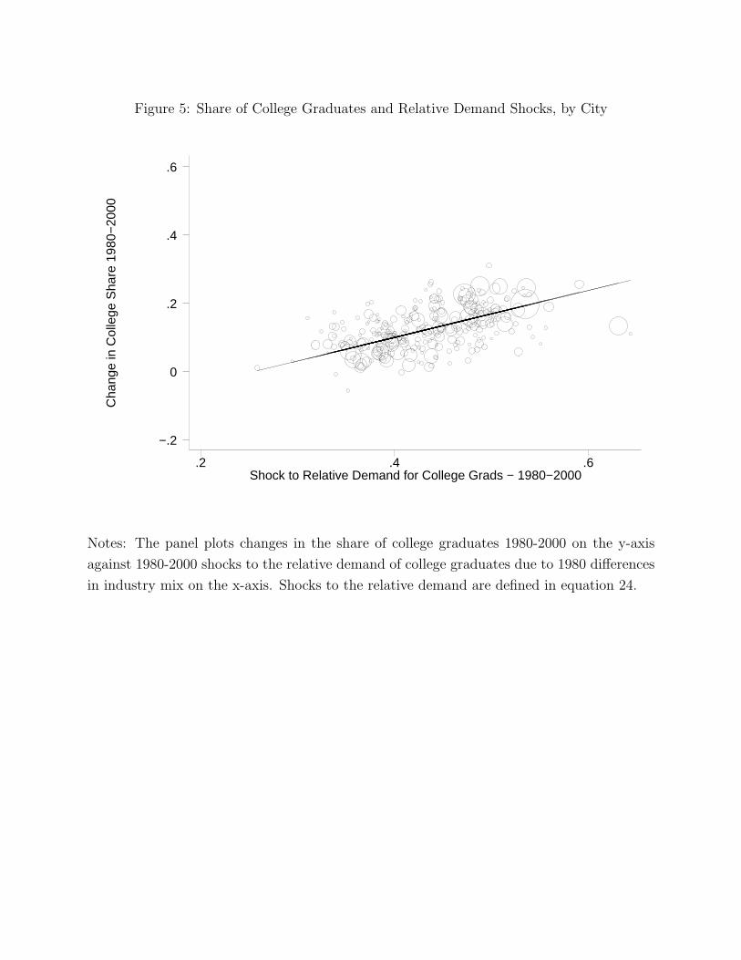
To determine whether relative demand or relative supply shocks are more important in
practice, I analyze the empirical relationship between changes in the college premium and
changes in the share of college graduates across metropolitan areas. My model indicates
that under the relative demand hypothesis, one should see a positive equilibrium relation-
ship between changes in the college premium and changes in the college share. Intuitively,
increases in the relative demand of college graduates in a city should result in increases in
their relative wage there. Under the relative supply hypothesis, one should not see such a
positive relationship. This test is related to the test proposed by Katz and Murphy (1992)
to understand nationwide changes in inequality.
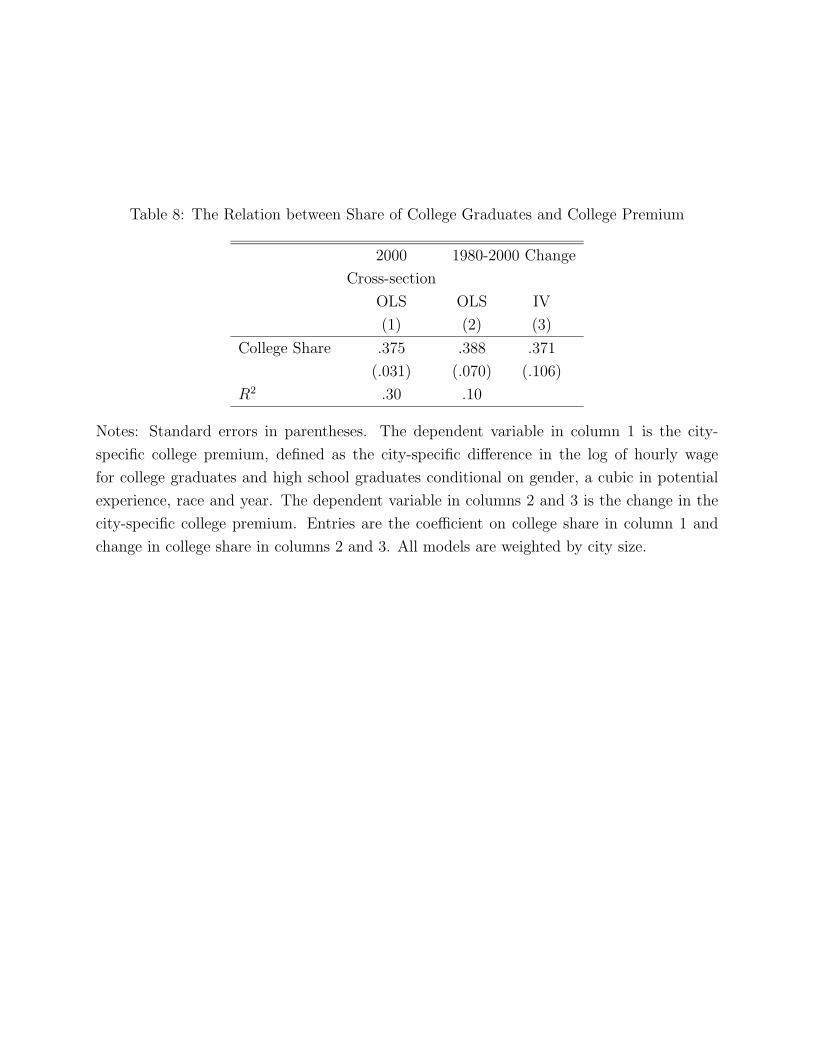
Consistent with relative demand shocks playing an important role, I find a strong positive
association between changes in the college premium and changes in the college share. While
this suggests that demand factors are important, it does not necessarily rule out supply
factors. As a second piece of evidence, I present instrumental variable estimates of the
relationship between changes in the college premium and changes in the college share based
on a shift-share instrument.5 The IV estimate establishes what happens to the college
premium in a city when the city experiences an increase in the number of college graduates
that is driven purely by an increase in the relative demand for college graduates. By contrast,
the OLS estimate establishes what happens to the college premium in a city when the city
experiences an increase in the number of college graduates that may be driven by either
demand or supply shocks. The comparison of the two estimates is therefore informative
about the relative importance of demand and supply shocks.
Overall, the empirical evidence is more consistent with the notion that relative demand
shocks are the main force driving changes in the number of skilled workers across metropoli-
tan areas.6 If this is true, the increase in well-being disparities between 1980 and 2000 is
significantly smaller than we previously thought based on the existing literature.7
4See also Kahn (1999).5The instrument is a weighted average of nationwide relative skilled employment growth by industry, with
weights reflecting the city-specific employment share in those industries in 1980.6This finding does not imply that amenities do not affect worker location decisions in general, nor it
implies that amenities do not affect location decisions of skilled and unskilled workers differently. Rather,
it implies that the differential change in the geographical location of skilled and unskilled workers in this
period is mostly driven by changes in the geographical differences in the availability of new skilled and
unskilled jobs, not by changes in the geographical differences in local amenities that are relevant to skilled
and unskilled workers.7I note that the exact magnitude of the increase in well-being disparities remains unkwown. While my
estimates indicate that the increase in well-being disparities is smaller than suggested by existing estimates,
a full account of changes in well-being disparities would require several additional pieces of information. For
3
My findings are consistent with previous studies that identify shifts in labor demand—
whether due to skill-biased technical change or product demand shifts across industries with
different skill intensities—as an important determinant of the increase in wage inequality
(for example, Katz and Murphy, 1992). But unlike the previous literature, my findings point
to an important role for the local component of these demand shifts. While in this paper I
take these local demand shifts as exogenous, future research should investigate the economic
forces that make skilled workers more productive in some parts of the country.8 The notion
that demand shocks are important determinants of population shifts is consistent with the
evidence in Blanchard and Katz (1992) and Bound and Holzer (2000).9 The specific finding
that variation in the college share is mostly driven by demand factors is consistent with the
argument made by Berry and Glaeser (2005) and Beaudry, Doms and Lewis (2008).
My results are also related to a series of papers by Pendakur (1998, 2002) and Lewbel and
Pendakur (forthcoming) on the correct use of price indexes on the measurement of inequality.
My approach is related to a paper by Black et al. (2010) which, along with earlier work by
Dahl (2002), criticizes the standard practice of treating the returns to education as uniform
across locations. They show that, in theory, the return to schooling is constant across
locations only in the special case of homothetic preferences, and argue that the returns
to education are empirically lower in high-amenity locations.10 My findings complement
the literature on consumption inequality, which has documented that income inequality is
higher and has grown faster than consumption inequality in many countries, including the
US. See Krueger, Perri, Pistaferri, Violante (2010) for a recent review of the evidence. In
principle, my estimates have the potential to provide an explanation for the slower increase
in consumption inequality in this period.11
From the methodological point of view, this paper illustrates the importance of accounting
for general equilibrium effects when thinking about the effects of group specific labor market
shocks. Labor economists often approach the analysis of labor market shocks using a partial
equilibrium analysis. However, this paper shows that a partial equilibrium analysis can miss
example, it would require estimates of relative changes in features of jobs other than wages (job amenities,
other forms of compensation, etc.) and estimates of the relative changes in housing wealth induced by
changes in housing prices. A full empirical treatment of these issues is complicated and is beyond the scope
of this paper.8See for example Moretti (2004a and 2004b) and Greenstone, Hornbeck and Moretti (forthcoming).9Chen and Rosenthal (forthcoming) document that jobs are the key determinant of mobility of young
individuals. Mobility of older individuals seems more likely to be driven by amenities.10In a related paper, Black et al. (2009) argue that estimates of the wage differences between blacks and
whites need to account for differences in the geographical location of different racial groups and develop a
theoretical model to understand when estimates of black-white earnings gap can be used to infer welfare
differences.11See also Duranton (2002 and 2008) on spatial wage disparities; Broda and Romalis (2009) who document
the distributional consequences of increased imports from China; Gordon (2009) and Gordon and Dew-Becker
(2005, 2007 and 2008); and Aguiar and Hurst (2007a and 2007b) who focus on the role of differential changes
in labor supply and leisure, by skill group.
4
important parts of the picture, since the endogenous reaction of factor prices and quantities
can significantly alter the ultimate effects of a shock. Because aggregate shocks to the labor
market are rarely geographically uniform, the geographic reallocation of factors and local
price adjustments are empirically important. It is difficult to fully understand aggregate
labor market changes—like changes in relative wages— if ignoring the spatial dimension of
labor markets. This paper shows that labor flows across localities and changes in local prices
have the potential to undo some of the direct effects of labor market shocks and this may
alter the implications for policy.
The rest of the paper is organized as follows. In Section 2, I describe how the official CPI
is calculated by the BLS and I propose two alternative CPI’s that allow for geographical
differences across skill groups. In Section 3, I present estimates of nominal and real college
premia. In Section 4, I present a simple model that can help interpreting the empirical
evidence. In Section 5, I discuss the different implications of the demand pull and supply
push hypotheses and present empirical evidence to distinguish the two. Section 6 concludes.
2 Cost of Living Indexes and the Location of Skilled
and Unskilled Workers
In this Section, I begin with some descriptive evidence on recent changes in the geo-
graphical location of skilled and unskilled workers and housing costs (subsection 2.1). I then
describe how the Bureau of Labor Statistics computes the official Consumer Price Index and
I propose two alternative measures of cost of living that account for geographical differences
(subsection 2.2). Finally, I use my measures of cost of living to document the differential
change in the cost of living experienced by high school and college graduates between 1980
and 2000 (subsection 2.3).
2.1 Changes in the Location of Skilled and Unskilled Workers
Throughout the paper, I use data from the 1980, 1990 and 2000 Censuses of Population.12
The geographical unit of analysis is the metropolitan statistical area (MSA) of residence.
Rural households in the Census are not assigned a MSA. In order to keep my wage regressions
as representative and as consistent with the previous literature as possible, I group workers
who live outside a MSA by state, and treat these groups as additional geographical units.
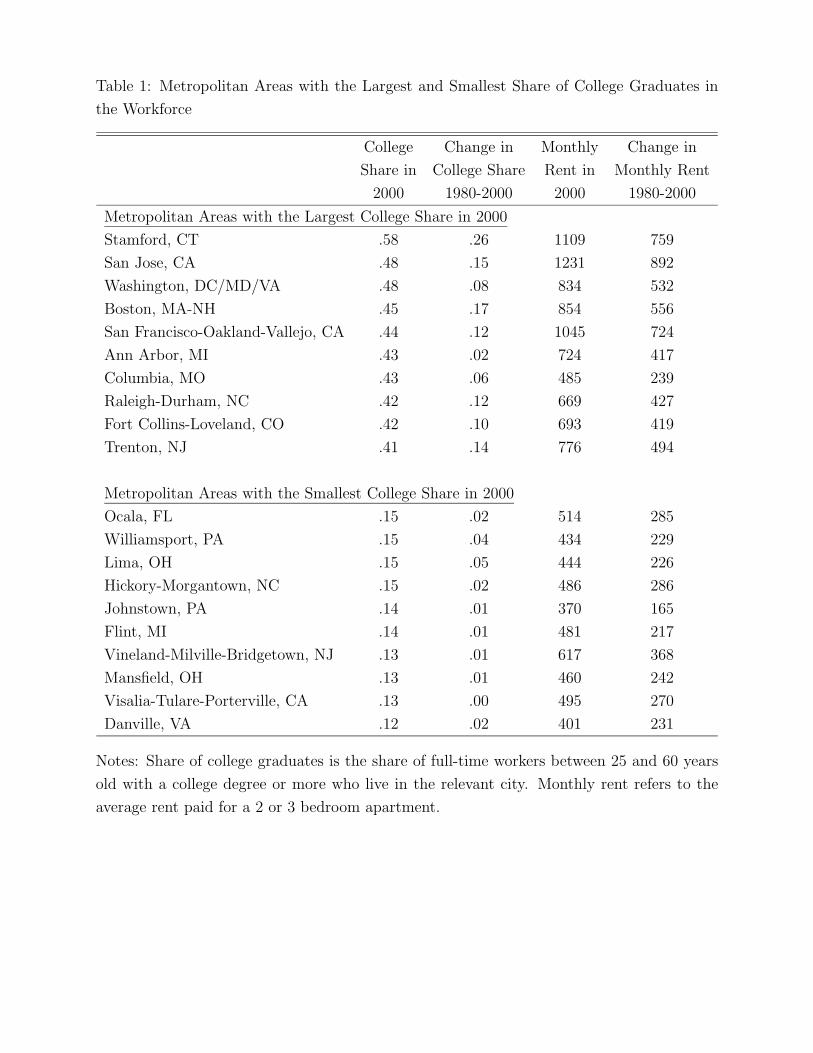
Table 1 documents differences in the fraction of college graduates across some US metropoli-
tan areas. Specifically, the top (bottom) panel reports the 10 cities with the highest (lowest)
fraction of workers with a college degree or more in 2000. Throughout the paper, college
graduates also include individuals with a post-graduate education. The metropolitan area
12Because my data end in 2000, my empirical analysis is not affected by the run-up in home prices during
the housing bubble years and the subsequent decline in home prices.
5
with the largest share of workers with a college degree among its residents is Stamford, CT,
where 58% of workers has a college degree or more. The fraction of college graduates in
Stamford is almost 5 times the fraction of college graduates in the city at the bottom on
the distribution—Danville, VA—where only 12% of workers have a college degree. Other
metropolitan areas in the top group include MSA’s with an industrial mix that is heavy in
high tech and R&D—such as San Jose, San Francisco, Boston and Raleigh-Durham—and
MSA’s with large universities— such as Ann Arbor, MI and Fort Collins, CO. Metropolitan
areas in the top panel have a higher cost of housing—as measured by the average monthly
rent for a 2 or 3 bedroom apartment—than metropolitan areas in the bottom panel. College
share and the cost of housing vary substantially not only in their levels across locations but
also in their changes over time. While cities like Stamford, Boston, San Jose and San Fran-
cisco experienced large increases in both the share of workers with a college degree and the
monthly rent between 1980 and 2000, cities in the bottom panel experienced more limited
increases.
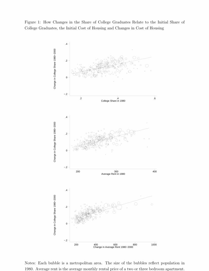
The relation between changes in the number of college graduates and changes in housing
costs is shown more systematically in Figure 1. The top panel shows how the 1980-2000
change in the share of college graduates relates to the 1980 share of college graduates.
The size of the bubbles reflect population in 1980. The positive relationship indicates that
college graduates are increasingly concentrated in metropolitan areas that have a large share
of college graduates in 1980. This relationship has been documented by Berry and Glaeser
(2005) and Moretti (2004), among others.13
The middle panel of Figure 1 shows how the 1980-2000 change in the share of college
graduates relates to the average cost of housing in 1980. The positive relationship indicates
that college graduates are increasingly concentrated in MSA’s where housing is initially
expensive.14 The bottom panel plots the 1980-2000 change in college share as a function of
the 1980-2000 change in the average monthly rental price. The positive relationship suggests
that the share of college graduates has increased in MSA’s where housing has become more
expensive.15
These relationships do not have a causal interpretation, but instead need to be inter-
preted as equilibrium relationships. Taken together, the panels in Figure 1 show that the
metropolitan areas that have experienced the largest increases in the share of college grad-
uates are the metropolitan areas where the average cost of housing in 1980 is highest and
13The regression of the 1980-2000 change in college share on the 1980 level in college share weighted by
the 1980 MSA size yields a coefficient equal to .460 (.032), indicating that a 10 percentage point difference in
the baseline college share in 1980 is associated with a 4.6 percentage point increase in college share between
1980 and 2000.14The regression of the 1980-2000 change in college share on the 1980 cost of housing weighted by the 1980
MSA size yields a coefficient equal to .0011 (.00006), indicating that a 100 dollar difference in the baseline
monthly rent in 1980 is associated with a 4.7 percentage point increase in college share between 1980 and
2000.15The regression yields a coefficient equal to .0003 (.00001).
6
also the areas where the average cost of housing has increased the most.
2.2 Local Consumer Price Indexes
A cost of living index seeks to measure changes over time in the amount that consumers
need to spend to reach a certain utility level or “standard of living.” Changes in the official
Consumer Price Index between period t and t + 1 as measured by the Bureau of Labor
Statistics are a weighted average of changes in the price of the goods in a representative
consumption basket. The basket is the original consumption basket at time t, and the
weights reflect the share of income that the average consumer spends on each good at time
t.16
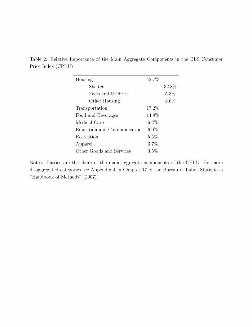
Table 2 shows the relative importance of the main aggregate components of the CPI for
all urban consumers, CPI-U, in 2000. The largest component by far is housing. In 2000,
housing accounts for more than 42% of the CPI-U. The largest sub-components of housing
costs are “Shelter” and “Fuel and Utilities”. The second and third main components of the
CPI-U are transportation and food. They only account for 17.2% and 14.9% of the CPI-U,
respectively. The weights of all the other categories are 6% or smaller.
Although most households in the US are homeowners, changes in the price of housing
are measured by the BLS using changes in the cost of renting an apartment (Poole, Ptacek
and Verbugge, 2006; Bureau of Labor Statistics, 2007). The rationale for using rental costs
instead of home prices is that rental costs are a better approximation of the user cost of hous-
ing. Since houses are an asset, their price reflects both the user cost as well as expectations
of future appreciation.
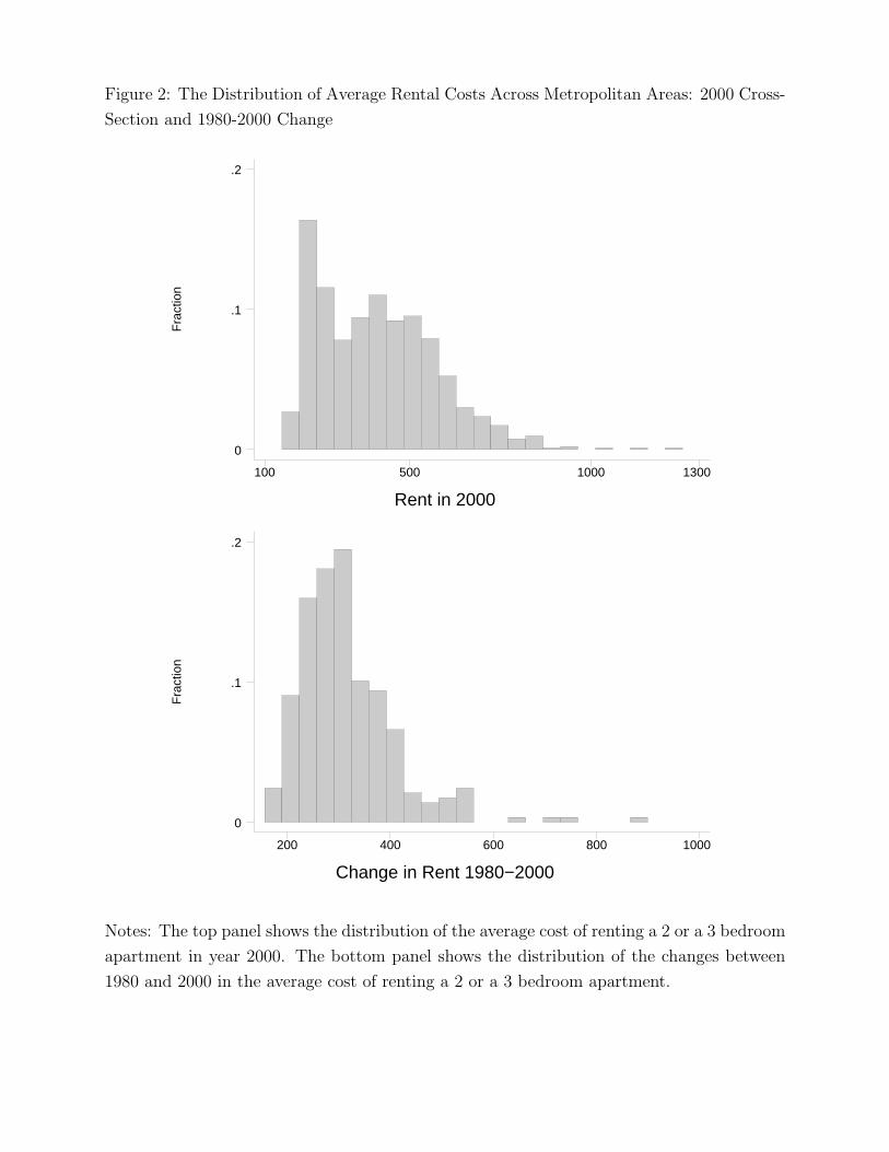
Rental costs vary significantly across metropolitan areas. For example, in 2000, the
average rental cost for a 2 or 3 bedroom apartment in San Diego, CA—the city at the 90th
percentile of the distribution—is $894. This rental cost is almost 3 times higher than the
rental cost for an equally sized apartment in Decatour, AL, the city at the 10th percentile.
Changes over time in rental costs also vary significantly across metropolitan areas. For
example, between 1980 and 2000, the rental cost increased by $165 in Johnstown, PA—one
of the cities at the bottom of the distribution—and by $892 in San Jose—one of the cities at
the top of the distribution. The distribution of average rental costs and changes in average
rental costs are shown in Figure 2.
Although the cost of living varies substantially across metropolitan areas, wage and in-
come are typically deflated using a single, nation-wide deflator, such as the CPI-U calculated
by the BLS. The use a nation-wide deflator is particularly striking in light of the fact that
16One well known problem with the CPI is the potential for substitution bias, which is the possibility that
consumers respond to price changes by substituting relatively cheaper goods for goods that have become
more expensive. While the actual consumption baskets may change, the CPI reports inflation for the original
basket. Details of the BLS methodology are described in Chapter 17 of the Handbook of Methods (BLS,
2007), titled “The Consumer Price Index”.
7
more than 40% of the CPI-U is driven by housing costs (Table 2), and that housing costs vary
so much across locations (Figure 2). To investigate the role of cost of living differences on
wage differences between skill groups, I propose two alternative CPI indexes that vary across
metropolitan areas. I closely follow the methodology that the Bureau of Labor Statistics
uses to build the official Consumer Price Index, but I generalize two of its assumptions.
Local CPI 1. First, I compute a CPI that allows for the fact that the cost of housing
varies across metropolitan areas. I call the resulting local price index “Local CPI 1”. Fol-
lowing the BLS methodology, I define Local CPI 1 as the properly weighted sum of local
cost of housing—with the average across cities normalized to 1 in 1980—and non-housing
consumption—normalized to 1 in 1980. I measure the cost of housing faced by an individual
in metropolitan area c in two ways. In my preferred specification, I follow the BLS method-
ology and I use rental costs. I assign the cost of housing to residents in a metropolitan area
based on the relevant average monthly rent. Specifically, I take the average of the monthly
cost of renting a 2 or 3 bedroom apartment among all renters in area c. As an alternative
way to measure cost of housing, in some models I use the price of owner occupied houses
instead of rental costs. Specifically, I take the average reported value of all 2 or 3 bedroom
owner occupied single family houses in area c. Both rental costs and housing prices are from
the Census of Population. As I discuss later, empirical results are not sensitive to measur-
ing housing costs using rental costs or housing prices. The price of non housing goods and
services is assumed to be the same in a given year, irrespective of location. This assumption
is relaxed in Local CPI 2.17
I describe the details of this approach in Appendix 1. It is important to note that this
methodology ensures that the deflator that I use for a given worker does not reflect the
increase in the cost of the apartment rented or the cost of the house owned by that specific
worker. Instead, it reflects the increase in the cost of housing experienced by residents in
the same city, irrespective of their own individual housing cost and irrespective of whether
they rent or own.
Local CPI 2. In local CPI 1, changes in the cost of housing can vary across localities,
but changes in the cost of non-housing goods and services are assumed to be the same
everywhere. While the cost of housing is the most important component of the CPI, the
price of other goods and services is likely to vary systematically with the cost of housing.
In cities where land is more expensive, production and retail costs are higher and therefore
the cost of many goods and services is higher. For example, a slice of pizza or a hair cut are
17The motivation for using 2 and 3 bedroom apartments is to keep the size of the apartment roughly similar.
I have experimented with variants of this selection rule. Estimates based only on 2 bedroom apartments are
similar to the ones presented below. Estimates based on data from the American Housing Survey that use
information on square footage to hold constant the exact size of the apartment also yield similar results. See
Section 3.3 below for details.
8
likely to be more expensive in New York city than in Indianapolis, since it is more expensive
to operate a pizza restaurant or a barber shop in New York city than Indianapolis.
Local CPI 2 allows for both the cost of housing and the cost of non-housing consumption
to vary across metropolitan areas. Systematic, high quality, city-level data on the price of
non-housing good and services are not available for most cities over a long time period. To
overcome this limitation, I use two alternative approaches. First, in my preferred specifica-
tion, I use the fact that the BLS releases a local CPI for a limited number of metropolitan
areas. This local CPI is not ideal because it is made available by the BLS only for 23 MSA’s
in the period under consideration and there are 315 MSA’s in the 2000 Census. Additionally,
it is normalized to 1 in a given year, thus precluding cross-sectional comparisons. However,
it can still be used to impute the part of local non-housing prices that varies systematically
with housing costs. The local CPI computed by the BLS for city c in year t is a weighted av-
erage of housing cost (HPct) and non-housing costs (NHPct): BLSct = wHPct +(1−w)NHPct
where w is the CPI weight used by BLS for housing. Non-housing costs can be divided in
two components:
NHPct = πHPct + vct (1)
where πHPct is the component of non-housing costs that varies systematically with housing
costs; and vct is the component that is orthogonal to housing costs. If π > 0 it means that
cities with higher cost of housing also have higher costs of non-housing goods and services.
I use the small sample of MSA’s for which a local BLS CPI is available to estimate π.18 I
then impute the systematic component of non-housing costs to all MSA’s, based on their
housing cost: E(NHPct|HPct) = π̂HPct. Finally, I compute “Local CPI 2” as a properly
weighted sum of the cost of housing, the component of non-housing costs that varies with
housing (π̂HPct), and the component of non-housing costs that does not vary with housing.
See Appendix 1 for more details.
As an alternative strategy to measure local variation in non-housing prices, I use data on
non-housing prices taken from the Accra dataset, which is collected by the Council for Com-
munity and Economic Research.19 The Accra data have both advantages and disadvantages.
On one hand, the Accra data are available for most cities, and therefore do not require any
imputation. Furthermore, the detail is such that price information is available at the level
of specific consumption goods and the price is not normalized to a base year. On the other
hand, the Accra data are available only for a very limited number of goods.20 Importantly,
18To do so, I first regress changes in the BLS local index on changes in housing costs: ∆BLSct = β∆HPct+
ect. Estimating this regression in differences is necessary because BLSct is normalized to 1 in a given year.
While cross-sectional comparisons based on BLSct are meaningless, BLSct does measure changes in prices
within a city. Once I have an estimate of β, I can calculate π̂ = β̂−w
1−w. Empirically, β̂ is equal to .588 (.001)
and π̂ is equal to .35 in 2000.19The data were generously provided by Emek Basker. Basker (2005) and Basker and Noel (2007) describe
the Accra dataset in detail.20Only 48 goods have prices that are consistently defined for the entire period under consideration. The
BLS basket includes more than 1000 goods.
9
the sample size for each good and city is quite small, so that local price averages are noisy.
Additionally, the set of cities covered changes over time. In practice, the empirical findings
based on the version of local CPI 2 that uses the imputation and those based on the version
of local CPI 2 that uses Accra data are similar.
In sum, local CPI 2 is more comprehensive than Local CPI 1 because it includes local
variation in both housing and non-housing costs, but it is has the limitation that non-housing
costs are imputed or come from Accra data. For this reason, in the next Section I present
separate estimates for Local CPI 1 and Local CPI 2.
2.3 Changes in the Cost of Living Experienced by Skilled and
Unskilled Workers Between 1980 and 2000
I now quantify the changes in the cost of living experienced by high school and college
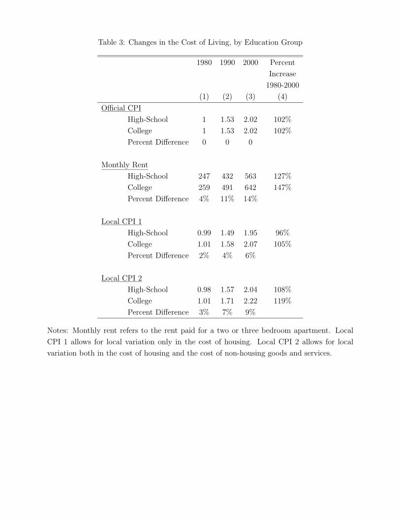
graduates between 1980 and 2000. The top panel of Table 3 shows changes in the official
CPI-U, as reported by the BLS, and normalized to 1 in 1980. This is the most widely used
measure of inflation, and it is the measure that is almost universally used to deflate wages
and incomes. According to this index, the price level doubled between 1980 and 2000. This
increase is—by construction—the same for college graduates and high school graduates.
The next panel shows the increase in the cost of housing faced by college graduates and
high school graduates. College graduates and high school graduates are exposed to very
different increases in the cost of housing. In 1980 the cost of housing for the average college
graduate is only 4% more than the cost of housing for the average high school graduate.
This gap grows to 11% in 1990 and reaches 14% by 2000. Column 4 indicates that housing
costs for high school and college graduates increased between 1980 and 2000 by 127% and
147%, respectively.
The third panel shows “Local CPI 1”, normalized to 1 in 1980 for the average household.21
The panel shows that in 1980 the overall cost of living experienced by college graduates is
only 2% higher than the cost of living experienced by high school graduates. This difference
increases to 6% by year 2000. The difference in Local CPI 1 between high school and college
graduates is less pronounced than the difference in monthly rent because Local CPI 1 includes
non-housing costs as well as housing costs.
The differential increase in cost of living faced by college graduates relative to high school
graduates is more pronounced when the price of non-housing goods and services is allowed
to vary across locations, as in the bottom panel. In the case of Local CPI 2, the cost of
living is 3% higher for college graduates relative to high school graduates in 1980 and 9%
in 2000. Column 4 indicates that the increase in the overall price level experienced by high
school graduates between 1980 and 2000 is 108%. The increase in the overall price level
experienced by college graduates between 1980 and 2000 is 119%.
21Here I use rental costs to measure housing costs. Using property values for owner occupied houses yields
similar results.
10
The relative increase in the cost of housing experienced by college graduates between
1980 and 2000 can be decomposed into a part due to geographical mobility and a part due
to the fact that already in 1980 college graduates are overrepresented in cities that experience
large increases in costs. Specifically, the 1980-2000 nationwide change in the cost of housing
experienced by skill group j (j=high school or college), can be written as
Pj2000 − Pj1980 =∑
c ωjc2000Pc2000 −∑
c ωjc1980Pc1980∑
c(ωjc2000 − ωjc1980)Pc2000 +∑
c ωjc1980(Pc2000 − Pc1980)
where ωjct is the share of workers in skill group j who live in city c in year t and Pct
is the cost of housing in city c in year t. The equation illustrates that the total change
in cost of housing is the sum of two components: a part due to the the change in the
share of workers in each city, given 2000 prices (∑
c(ωjc2000 − ωjc1980)Pc2000); and a part due
to the differential change in the cost of housing across cities, given the 1980 geographical
distribution (∑
c ωjc1980(Pc2000 − Pc1980)). The change in cost of housing of college graduates
relative to high school graduates is therefore the difference of these two components for
college graduates and high school graduates.
Empirically, I find that both factors are important. About 43% of the total increase
in cost of housing of college graduates relative to high school graduates is due to the first
component (geographical mobility of college graduates toward expensive cities), and 57% is
due to the second component (larger cost increase in cities that have many college graduates
in 1980).
3 Nominal and Real Wage Differences
In this Section, I estimate how much of the increase in nominal wage differences between
college graduates and high school graduates is accounted for by differences in the cost of
living. In particular, in Section 3.1 I show estimates of the college premium in nominal and
real terms. In Sections 3.2 and 3.3 I discuss whether my estimates are biased by the presence
of unobserved worker characteristics or unobserved housing characteristics. In Section 3.4 I
show estimates of the college premium in real terms based on an alternative local CPI that
varies not just by metropolitan area, but also by skill level within metropolitan area.
3.1 Main Estimates
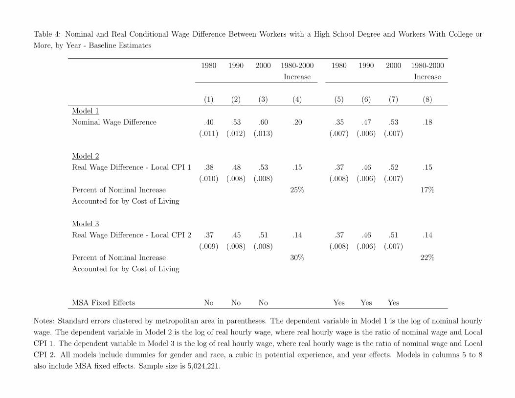
Model 1 in the top panel of Table 4 estimates the conditional nominal wage difference
between workers with a high school degree and workers with college or more, by year. Esti-
mates in columns 1 to 4 are from a regression of the log nominal hourly wage on an indicator
for college interacted with an indicator for year 1980, an indicator for college interacted
with an indicator for year 1990, an indicator for college interacted with an indicator for year
2000, years dummies, a cubic in potential experience, and dummies for gender and race.
11
Estimates in columns 5 to 8 are from models that also include MSA fixed effects. Entries
are the coefficients on the interactions of college and year and represent the conditional wage
difference for the relevant year. The sample includes all US born wage and salary workers
aged 25-60 who have worked at least 48 weeks in the previous year.22
My estimates in columns 1 to 4 indicate that the conditional nominal wage difference
between workers with a high school degree and workers with college or more has increased
significantly. The difference is 40% in 1980 and rises to 60% by 2000. Column 4 indicates
that this increase amounts to 20 percentage points. This estimate is generally consistent
with the previous literature (see, for example, Table 3 in Katz and Autor, 1999).
Models 2 and 3 in Table 4 show the conditional real wage differences between workers
with a high school degree and workers with college or more. To quantify this difference, I
estimate models that are similar to Model 1, where the dependent variable is the nominal
wage divided by Local CPI 1 (in Model 2) or by Local CPI 2 (in Model 3). Two features are
noteworthy. First, the level of the conditional college premium is lower in real terms than
in nominal terms in each year. For example, in 2000 the conditional difference between the
wage for college graduates and high school graduates is .60 in nominal terms and only .53 in
real terms when Local CPI 1 is used as deflator. The difference is smaller—.51 percentage
points—when Local CPI 2 is used as deflator. Second, the increase between 1980 and 2000
in college premium is significantly smaller in real terms than in nominal terms. For example,
using Local CPI 1, the 1980-2000 increase in the conditional real wage difference between
college graduates and high school graduates is 15 percentage points. In other words, cost of
living differences as measured by Local CPI 1 account for 25% of the increase in conditional
inequality between college and high school graduates between 1980 and 2000 (column 4).
The effect of cost of living differences is even more pronounced when the cost of living is
measured by Local CPI 2. In this case, the increase in the conditional real wage difference
between college graduates and high school graduates is 14 percentage points. This implies
that cost of living differences as measured by Local CPI 2 account for 30% of the increase
in conditional wage inequality between college and high school graduates between 1980 and
2000 (column 4).
When I control for fixed effects for metropolitan areas in columns 5-8, the nominal college
premium is slightly smaller, but the real college premium is generally similar. The increase
in the college premium is 18 percentage points when measured in nominal terms, and 14-15
percentage points when measured in real terms, depending on whether CPI 1 or CPI 2 is used
as deflator. After conditioning on MSA fixed effects, cost of living differences account 22%
of the increase in conditional inequality between college and high school graduates between
1980 and 2000 when CPI 2 is used as a deflator (column 8).
22The sample includes both men and women. This may be a concern, since in a recent paper by Black et
al. (2010) shows that female labor force participation is different in different cities. At the end of this sub-
section, I discuss a number of alternative specifications, including one when I estimate the college premium
for men and women separetely. Estimates by gender are similar to those obtained from the pooled sample.
12
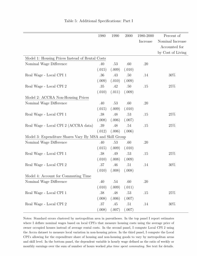
In Tables 5 and 6 I present the results from several alternative specifications. I begin in
the top panel of Table 5 by showing estimates where I deflate nominal wages based on local
CPI’s that measure housing costs using the average price of owner occupied houses instead of
average rental costs. In particular, as discussed in Section 2.2, I measure local housing prices
by taking the average reported property value of all 2 or 3 bedroom single family owner
occupied houses in the relevant MSA. In the second panel, I compute Local CPI 2 using the
Accra dataset described above to measure local variation in non-housing prices. (See Section
2.2 for details). In the third panel, I compute the Local CPI’s allowing for the expenditure
share of housing and non-housing goods to vary by metropolitan areas and skill level. (See
Appendix 1 for more details). In the bottom panel, I consider the possibility that commuting
distance may vary differentially for high school and college graduates. For example, it is
possible that increases in the number of college graduates in some cities lead high school
graduates to live farther away from job locations. To account for possible differential changes
in commuting times, I re-estimate the baseline model where the dependent variable is wage
per hour worked or spent commuting. In the baseline estimates, I calculate hourly wage by
taking the ratio of weekly or monthly earnings over the sum of number of hours worked. By
contrast, here I calculate hourly wage by taking the ratio of weekly or monthly earnings over
the sum of number of hours worked plus time spent commuting.
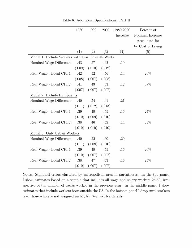
In the top panel of Table 6, I show estimates based on a sample that includes all wage
and salary workers 25-60, irrespective of the number of weeks worked in the previous year. In
the middle panel, I show estimates that include workers born outside the US. In the bottom
panel I drop rural workers (i.e. those who are not assigned an MSA).
In general, estimates in Tables 5 and 6 are not very different from the baseline estimates
in Table 4. The inclusion of workers with less than 48 weeks of work results in a slightly
larger percent of the nominal increase in inequality being accounted for by differences in cost
of living. I have performed several additional robustness checks that are not reported in the
Table due to space limitations and that are generally consistent with the estimates reported
in the Table.23
23For example, when I allow for the effect of experience, race, and gender to vary over time by controlling
for the interaction of year with gender, race and a cubic in experience, results are similar to Table 4. When
I estimate separate models for male and females, results are generally similar. When I estimate separate
models for workers with less than 20 years of experience and workers with more than 20 years of experience,
I find that the college premium seems to be smaller, and to have grown less—both in nominal and real
terms—for workers with higher levels of potential experience. Estimates where the dependent variable is the
log of weekly or yearly earnings are also generally consistent with Table 4. Finally, my estimates are not
very sensitive to the exclusion of outliers (defined as the top 1% and the bottom 1% of each year’s wage
distribution).
13
3.2 Worker Ability
One might be concerned about unobserved differences in worker ability. Models in Tables
4 and 5 control for standard demographics, but not for worker ability. Ability of college
graduates and high school graduates is likely to vary across metropolitan areas (Combes,
Duranton and Gobillon, 2008). Note that what may cause bias is not the mere presence
of cross-sectional differences across cities in the relative average ability of college graduates
and high school graduates. My estimates of the change in college premium in real terms
are biased if the change over time in the average ability of college graduates relative to
high school graduates in a given city is systematically related to changes over time in cost of
living in that city. The direction of the bias is a priori not obvious. If the average unobserved
ability of college graduates relative to high school graduates grows more (less) in expensive
cities compared to less expensive cities, then the estimates of the real college premia in Table
4 are biased downward (upward).
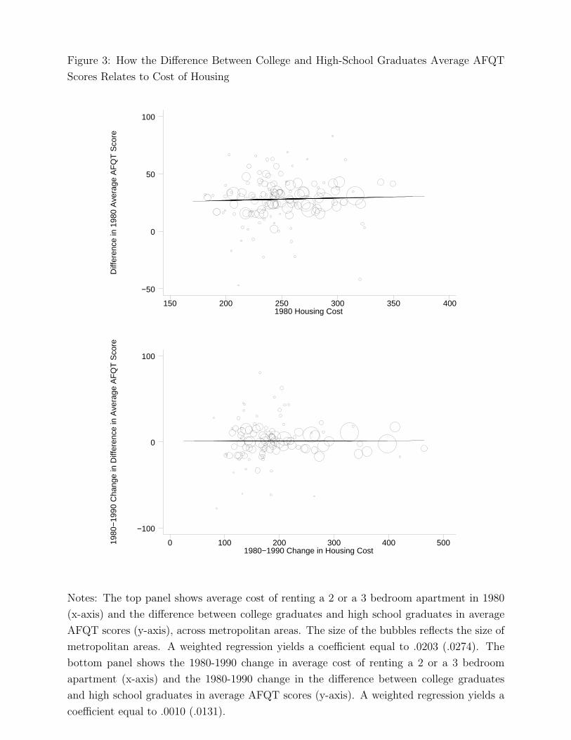
While I can not completely rule out the possibility of unmeasured worker differences, in
Figure 3 I provide some evidence on the relationship between one measure of worker ability
and housing costs. Specifically, I use NLSY data to relate the difference in average AFQT
scores between college graduates and high-school graduates across metropolitan areas to the
cost of housing across metropolitan areas.24
The top panel in the Figure shows average cost of renting a 2 or a 3 bedroom apart-
ment in 1980 on the x-axis against the difference between college graduates and high school
graduates in average AFQT score percentiles on the y-axis, across metropolitan areas. The
level of observation is a metropolitan area. The size of the bubbles reflects the size of the
metropolitan areas. Not surprisingly, the Figures shows that in most metropolitan areas
college graduates have significantly higher average AFQT score than high school graduates.
However, this difference does not appear to be systematically associated with housing costs.
A weighted regression of the difference between college graduates and high school graduates
in average AFQT scores on the average cost of renting a 2 or a 3 bedroom apartment yields
a coefficient equal to .0203 (.0274).
The bottom panel of the Figure shows the same relationship in changes over time. Specif-
ically, the graph shows the 1980-1990 change in average cost of renting a 2 or a 3 bedroom
apartment and the 1980-1990 change in the difference between college graduates and high
school graduates in average AFQT scores. A weighted regression yields a coefficient equal
to .0010 (.0131).
In sum, the Figure indicates that both in a cross section of cities, as well as in changes
over time for the same city, differences in ability between skill groups are generally orthogonal
to housing costs. This finding is consistent with the evidence in Glaeser and Mare (2001).
24My data contain AFQT score percentiles in 1980 and 1989. I merge these data with Census data on
housing costs for 1980 and 1990. Like in Section 3.1, housing costs are measured using the average cost of
renting a 2 or 3 bedroom apartment in the relevant MSA. I do not have AFQT scores in 2000.
14
3.3 Housing Quality
A second concern is the possibility that the the changes in housing costs faced by skilled
and unskilled workers reflect not just changes in cost of living, but also differential changes
in the quality of housing. This could bias my estimates of the relative increase in the cost
of living experienced by different skill groups, although the direction of the bias is not a
priori obvious. One the one hand, the relative increase in the cost of housing experienced by
college graduates may be overestimated if apartments in cities with many college graduates
are subject to more quality improvements between 1980 and 2000 than apartments in cities
with many high school graduates. In this case part of the additional increase in the rental
cost in cities with many college graduates relative to cities with many high school graduates
reflects differential quality improvements. Take, for example, features like the presence of a
fireplace, or quality of the kitchen and bathrooms. If these features have improved more in
cities with many college graduates, I may be overestimating the relative increase in cost of
living experienced by college graduates.
On the other hand, the relative increase in the cost of housing faced by college graduates
may be underestimated if apartments in cities with many high school graduates experience
more quality or size improvements. Take, for example, features like the size of an apart-
ment25, or the availability of a garden, a garage, or a porch. The average apartment in
New York or San Francisco is likely to be smaller than the average apartment in Houston or
Indianapolis and it is also less likely to have a garden, a garage or a porch. Moreover, these
features are less likely to have increased between 1980 and 2000 in New York or San Francisco
than in Houston or Indianapolis. Since the share of college graduates has increased more in
denser and more expensive cities, the true change in quality-adjusted per-square-foot price
faced by college graduates can in principle be larger than the one that I measure.
While I can not completely rule out the possibility of unmeasured quality differences,
here I present evidence based on a rich set of observable quality differences. I use data from
the American Housing Survey, which includes richer information on housing quality than
the Census of Population. Available quality variables include exact square footage, number
of rooms, number of bathrooms, indicators for the presence of a garage, a usable fireplace, a
porch, a washer, a dryer, a dishwasher, outside water leaks, inside water leaks, open cracks
in walls, open cracks in ceilings, broken windows, presence of rodents, and a broken toilet in
the last 3 months.26
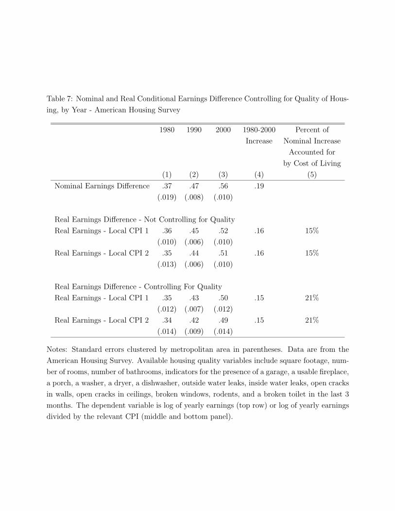
I begin by reproducing the baseline estimates that do not control for quality. Nominal
estimates based on the American Housing Survey in the top panel of Table 7 are generally
25Although my measure of housing cost is the average rent for apartments with a fixed number of bedrooms,
exact square footage may vary.26Each year, the American Housing Survey has a sample size that is significantly smaller than the sample
size in the Census. To increase precision, instead of taking only 1980, 1990 and 2000, I group years 1978-1984,
1988-1992 and 1998-2002 together.
15
similar to the corresponding baseline estimates based on the Census reported in Table 4.27
These estimates indicate that the nominal college premium increases by 19 percentage points
between 1980 and 2000. In the middle panel I estimate the real college premium, without
controlling for housing quality. Finally, in the bottom panel I re-estimate the same model
holding constant all available measures of housing quality. As before, I measure housing
cost using the rental price for renters. But, unlike before, I first regress housing costs on the
vector of observable housing characteristics. The residual from this regression represents the
component of the cost of housing that is orthogonal to my measures of dwelling quality. The
bottom panel of Table 7 shows how the baseline estimates change when I use the properly
renormalized residual as a measure of housing cost in my local CPI 1 and CPI 2. The
comparison of the middle and the bottom panels suggests that the 1980-2000 increase in real
college premium estimated controlling for quality is smaller than the corresponding increase
in the real college premium estimated without controlling for quality. Specifically, column
4 indicates that the increase in real college premium estimated controlling for quality is
15 percentage points. The corresponding estimate that does not control for quality is 16
percentage points.
In sum, though I can not completely rule out the possibility of unmeasured quality
differences, Table 7 indicates that controlling for a rich vector of observable quality differences
results in differences between nominal and real college premium that are slightly larger than
the baseline differences. This result is consistent with estimates in Malpezzi, Chun and
Green (1998).
3.4 An Alternative Measures of Local Cost of Living
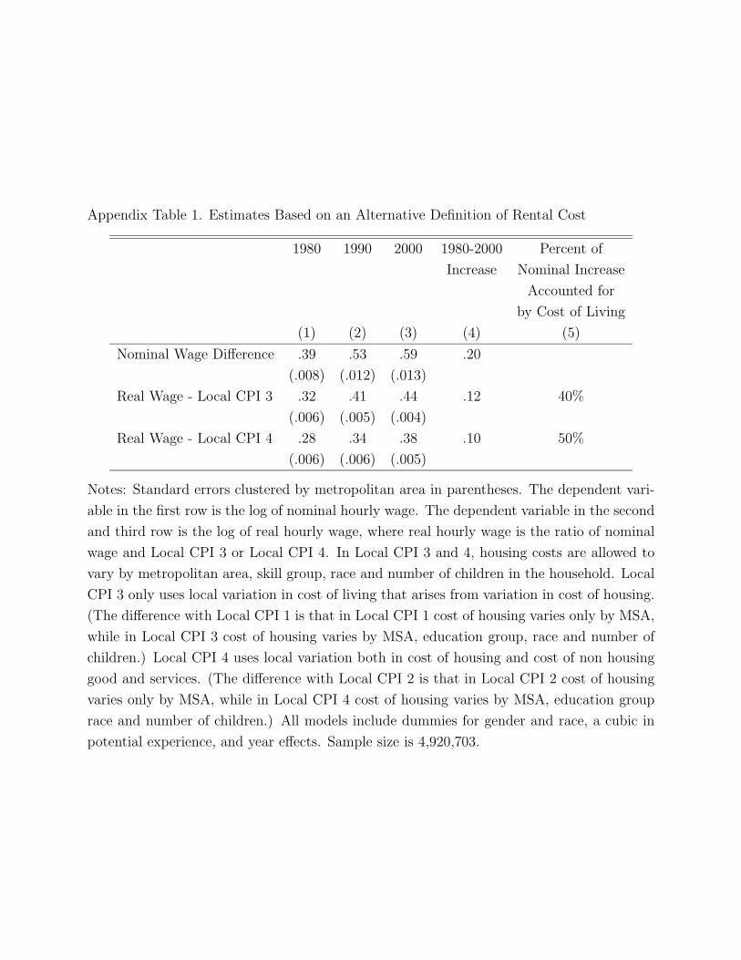
My estimates in Section 3.1 are based on a definition of cost of living where the housing
component of cost of living varies only by metropolitan area. In Appendix Table A1 I show
how my estimates change when an alternative definition of cost of living is adopted. In par-
ticular, I allow for the cost of housing experienced by different individuals to vary depending
not just on their city of residence, but also on their education level, family structure and
race. The idea is that, within a city, not all households necessarily use the same type of
housing. Allowing for the cost of housing faced by different demographic groups in a given
city to be different may matter if tastes and budget constraints differ across groups, so that
the type of housing that is used by some demographic groups in a city is not identical to the
one that is used by other groups. In this case, the group-specific rental cost is measured as
the predicted value from a regression of rental cost on identifiers for metropolitan area, edu-
cation group, number of children, race and interactions, where the regression is estimated on
the sample of renters of 2 or 3 bedroom apartments and the predicted values are calculated
27Unlike Table 4, the dependent variable here is log of yearly earnings. In the American Housing Survey
there is less information on number of hours worked than in the Census. Since college graduates work longer
hours, the estimated nominal college premium is slightly smaller than in Table 4.
16
for all households. Local CPI 3 only uses local variation in cost of living that arises from
variation in predicted cost of housing. Local CPI 4 uses local variation both in predicted
cost of housing and cost of non housing good and services. Estimates in Appendix Table 1
indicate that, relative to Table 4, a larger share of the increase in nominal wage differences
appears to be accounted for by cost of living differences.28
4 A Simple Framework
In the previous Section, I have shown that over the 1980-2000 period, real wage inequal-
ity has grown less than nominal wage inequality. Does this mean that the large increases
in nominal inequality have not translated into large increases in well being inequality? Not
necessarily. If amenities differ across cities, changes in real wages do not necessarily equal
changes in well-being. In this Section, I use a simple general equilibrium model to inves-
tigate the implications of my empirical findings for changes in well-being disparities. The
implications are different depending on the reasons for the increase in the share of college
graduates in expensive cities. I consider two alternative explanations for such an increase.
1. First, it is possible that skilled workers move to expensive cities because the relative demand
of skilled labor increases in expensive cities, as firms located in these cities increasingly
seek to hire skilled labor. This can be due to localized skill-biased technical change
or positive shocks to the demand faced by industries that employ skilled workers and
are located in expensive cities (for example, high tech, finance, etc.). In this case, the
increase in utility disparity between skilled and unskilled workers is smaller than the
increase in nominal wage disparity, because the higher nominal wage of skilled workers
is in part off-set by higher cost of living in the cities where skilled jobs are located.
2. Alternatively, it is possible that skilled workers move to expensive cities because the
relative supply of skilled labor increases in expensive cities, as skilled workers are in-
creasingly attracted by amenities located in those cities. In this case, a higher cost
of housing reflects consumption of desirable local amenities. Since this consumption
arguably generates utility, it is possible to have large increases in utility disparities
even when increases in real wage disparities are limited.
To formalize these two alternative hypotheses, and what they imply for inequality in
utility and wages, I consider a simple general equilibrium model of the labor and housing
market. The model is a generalization of the Roback (1982, 1988) model and has two types
of workers, skilled workers (type H) and unskilled workers (type L). Like in Roback, workers
and firms are mobile and choose the location that maximizes utility or profits. But unlike
28An obvious concern is the possibility of differential changes in the unmeasured quality of housing for
college graduates and high school graduates within a city. I have repeated the analysis of Table 7 and found
results that are generally similar.
17
Roback, the elasticity of local labor supply is not infinite, so that productivity and amenity
shocks are not always fully capitalized into land prices. This allows shocks to the relative
demand and relative supply of skilled workers to have different effects on the utility of skilled
and unskilled workers.
For simplicity of exposition, I model the two explanations as mutually exclusive. In the
empirical tests that seek to distinguish between the two explanations (Section 5), I allow for
the possibility that both demand and supply forces are at play at the same time.
4.1 Assumptions and Equilibrium
I assume that each city is a competitive economy that produces a single output good y
which is traded on the international market, so that its price is the same everywhere and set
equal to 1. Like in Roback, I abstract from labor supply decisions and I assume that each
worker provides one unit of labor, so that local labor supply is only determined by workers’
location decisions. The indirect utility of skilled workers in city c is assumed to be
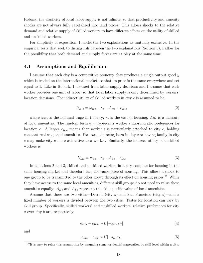
UHic = wHc − rc + AHc + eHic (2)
where wHc is the nominal wage in the city; rc is the cost of housing; AHc is a measure
of local amenities. The random term eHic represents worker i idiosyncratic preferences for
location c. A larger eHic means that worker i is particularly attached to city c, holding
constant real wage and amenities. For example, being born in city c or having family in city
c may make city c more attractive to a worker. Similarly, the indirect utility of unskilled
workers is
ULic = wLc − rc + ALc + eLic (3)
In equations 2 and 3, skilled and unskilled workers in a city compete for housing in the
same housing market and therefore face the same price of housing. This allows a shock to
one group to be transmitted to the other group through its effect on housing prices.29 While
they have access to the same local amenities, different skill groups do not need to value these
amenities equally: AHc and ALc represent the skill-specific value of local amenities.
Assume that there are two cities—Detroit (city a) and San Francisco (city b)—and a
fixed number of workers is divided between the two cities. Tastes for location can vary by
skill group. Specifically, skilled workers’ and unskilled workers’ relative preferences for city
a over city b are, respectively
eHia − eHib ∼ U [−sH , sH ] (4)
and
eLia − eLib ∼ U [−sL, sL] (5)
29It is easy to relax this assumption by assuming some residential segregation by skill level within a city.
18
The parameters sH and sL characterize the importance of idiosyncratic preferences for
location and therefore the degree of labor mobility. If sH is large, for example, it means that
preferences for location are important for skilled workers and therefore their willingness to
move to arbitrage away real wage differences or amenity differences is limited. On the other
hand, if sH is small, preferences for location are not very important and therefore skilled
workers are more willing to move in response to differences in real wages or amenities. In
the extreme, if sH = 0 skilled workers’ mobility is perfect.
A worker chooses city a if and only if eia − eib > (wb − rb) − (wa − ra) + (Ab − Aa). In
equilibrium, the marginal worker needs to be indifferent between living in Detroit and San
Francisco. This implies that skilled workers’ labor supply is upward sloping, with the slope
that depends on s. For example, the supply of skilled workers in San Francisco is:
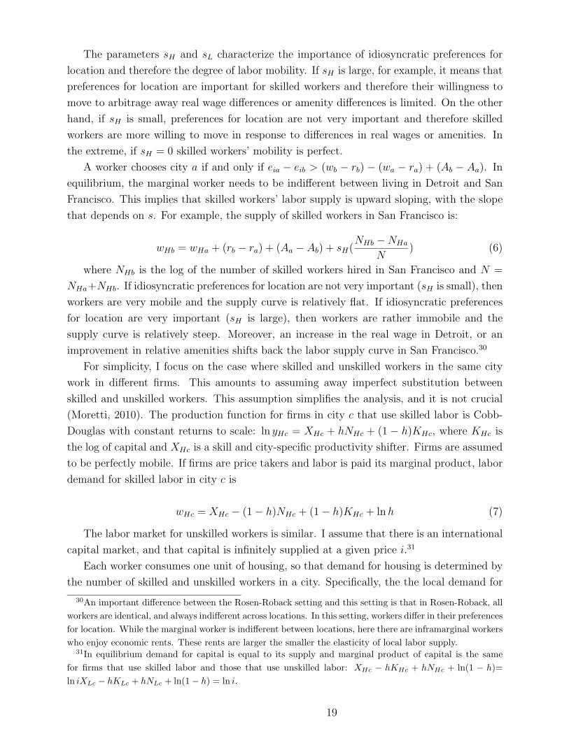
wHb = wHa + (rb − ra) + (Aa − Ab) + sH(NHb − NHa
N) (6)
where NHb is the log of the number of skilled workers hired in San Francisco and N =
NHa+NHb. If idiosyncratic preferences for location are not very important (sH is small), then
workers are very mobile and the supply curve is relatively flat. If idiosyncratic preferences
for location are very important (sH is large), then workers are rather immobile and the
supply curve is relatively steep. Moreover, an increase in the real wage in Detroit, or an
improvement in relative amenities shifts back the labor supply curve in San Francisco.30
For simplicity, I focus on the case where skilled and unskilled workers in the same city
work in different firms. This amounts to assuming away imperfect substitution between
skilled and unskilled workers. This assumption simplifies the analysis, and it is not crucial
(Moretti, 2010). The production function for firms in city c that use skilled labor is Cobb-
Douglas with constant returns to scale: ln yHc = XHc + hNHc + (1 − h)KHc, where KHc is
the log of capital and XHc is a skill and city-specific productivity shifter. Firms are assumed
to be perfectly mobile. If firms are price takers and labor is paid its marginal product, labor
demand for skilled labor in city c is
wHc = XHc − (1 − h)NHc + (1 − h)KHc + ln h (7)
The labor market for unskilled workers is similar. I assume that there is an international
capital market, and that capital is infinitely supplied at a given price i.31
Each worker consumes one unit of housing, so that demand for housing is determined by
the number of skilled and unskilled workers in a city. Specifically, the the local demand for
30An important difference between the Rosen-Roback setting and this setting is that in Rosen-Roback, all
workers are identical, and always indifferent across locations. In this setting, workers differ in their preferences
for location. While the marginal worker is indifferent between locations, here there are inframarginal workers
who enjoy economic rents. These rents are larger the smaller the elasticity of local labor supply.31In equilibrium demand for capital is equal to its supply and marginal product of capital is the same
for firms that use skilled labor and those that use unskilled labor: XHc − hKHc + hNHc + ln(1 − h)=
ln iXLc − hKLc + hNLc + ln(1 − h) = ln i.
19
housing is the sum the demand of skilled workers and the demand of unskilled workers. For
example, in city b:
rb =(2sHsL)
(sH + sL)−
(2sHsL)(NHb + NLb)
N(sH + sL)−
sL(wHa − wHb − ra)
(sL + sH)−
sH(wLa − wLb − ra)
(sL + sH)(8)
To close the model, I assume that the supply of housing is
rc = z + kcNc (9)
where Nc = NHc + NLc is the number of housing units in city c, which is the same as the
number of workers. The parameter kc characterizes the elasticity of the supply of housing.
I assume that this parameter is exogenously determined by geography and local land reg-
ulations. In cities where geography and regulations make it easy to build new housing, kc
is small. In the extreme case where there are no constraints to building new houses, the
supply curve is horizontal, and kc is zero. In cities where geography and regulations make
it difficult to build new housing, kc is large. In the extreme case where it is impossible to
build new houses, the supply curve is vertical, and kc is infinite.32
In period 1, the two cities are assumed to be identical. Equilibrium in the labor market
is obtained by equating equations 6 and 7 for each city. Equilibrium in the housing market
is obtained by equating equations 8 and 9. I consider two scenarios for period 2. In the first
scenario, the relative demand of skilled workers increases in one of the two cities (Section
4.2). In the second scenario, the relative supply of skilled workers increases in one of the
two cities (Section 4.3). The implications of the two scenarios for the empirical analysis are
summarized in Section 4.4.
4.2 Increase in the Relative Demand of Skilled Labor
Here I consider the case where the productivity of skilled workers increases relative to
the productivity of unskilled workers in San Francisco. Nothing happens to the productivity
of unskilled workers in San Francisco and the productivity of skilled and unskilled workers
in Detroit. In other words, the relative demand for skilled labor increases in San Francisco.
The amenities in the two cities are identical and fixed. Formally, I assume that in period
2, the productivity shifter for skilled workers in San Francisco is higher than in period 1:
XHb2 = XHb1 + ∆, where ∆ > 0 represents a positive, localized, skill-biased productivity
shock. I have added subscripts 1 and 2 to denote periods 1 and 2. The dot-com boom
32A limitation of equation 9 is housing production does not involve the use of any local input. Roback
(1982) and Glaeser (2008), among others, discuss spatial equilibrium in the case where housing production
involves the use of local labor and other local inputs. Moreover, equation 9 ignores the durability of housing.
Glaeser and Gyourko (2001) point out that once built, the housing stock does not depreciate quickly and
this introduces an asymmetry between positive and negative demand shocks. In particular, when demand
declines, the quantity of housing cannot decline, at least in the short run.
20
experienced by the San Francisco Bay Area is arguably an example of such a localized skill
biased shock. Driven by the advent of the Internet and the agglomeration of high tech firms
in the area, the demand for skilled workers increased significantly (relative to the demand
for unskilled workers) in San Francisco in the second half of the 1990s.33
Because skilled workers in San Francisco have become more productive, their nominal
wage increases by an amount ∆/h, proportional to the productivity increase. Attracted
by this higher productivity, some skilled workers leave Detroit and move to San Francisco.
Following this inflow of skilled workers, the cost of housing in San Francisco increases by
rb2 − rb1 =sLNkb∆
h(kaNsH + 2sHsL + kaNsL + kbNsH + kbNsL)≥ 0 (10)
In Detroit, the cost of housing declines by the same amount because of out-migration.
In San Francisco, real wages of skilled workers increase by
The productivity shock creates winners and losers. Skilled workers in both cities and
landowners in San Francisco benefit from the productivity increase. Inframarginal unskilled
workers in San Francisco are negatively affected, and inframarginal unskilled workers in
Detroit are positively affected.35 The exact magnitude of the changes in utility for skilled and
unskilled workers and for landowners crucially depends on which of the three factors—skilled
labor, unskilled labor or land—is supplied more elastically at the local level. Specifically, the
incidence of the shock depends on the elasticities of labor supply of the two groups (which
are governed by the preference parameters sH and sL) and the elasticities of housing supply
in the two cities (which are governed by the parameters ka and kb). Moretti (forthcoming)
provides detailed discussion of the incidence and welfare consequences of relative demand
shocks.
The model also illustrates that a non-degenerate equilibrium is possible. After a shock
that makes one group more productive, both groups are still represented in both cities. This
conclusion hinges upon the assumption of a less than infinite elasticity of local labor supply.36
Firms are indifferent between cities because they make the same profits in both cities. While
labor is now more expensive in San Francisco, it is also more productive there. Because firms
produce a good that is internationally traded, if skilled workers weren’t more productive,
employers would leave San Francisco and relocate to Detroit.37
4.3 Increase in the Relative Supply of Skilled Labor
In the case of demand pull described above, the number of skilled workers in San Francisco
increases because the relative demand of skilled workers increases. I now turn to the opposite
case, where the number of skilled workers in San Francisco increases because the relative
supply of skilled workers in San Francisco increases.
Specifically, I consider what happens when San Francisco becomes relatively more desir-
able for skilled workers compared to Detroit. I assume that in period 2, the amenity level
35Although inframarginal unskilled workers in San Francisco are made worse off by the decline in their real
wage, they are still better off in San Francisco than in Detroit because of their preference for San Francisco.36In the absence of individual preferences for location, no unskilled worker would remain in San Francisco
and the equilibrium would be characterized by complete geographic segregation of workers by skill level.
This is not realistic, since in reality we never observe cities that are populated by workers of only one type.37An assumption of this model is that skilled and unskilled workers are employed by different firms, so
that the labor market is segregated by skill within a city. This assumption effectively rules out imperfect
substitutability between skilled and unskilled labor. In a more general setting, skilled and unskilled workers
work in the same firm. The qualitative results generalize, but the equilibrium depends on the degree of
imperfect substitution between skilled and unskilled labor. Specifically, complementarity between skilled
and unskilled workers implies that the marginal product of unskilled workers increases in the number of
skilled workers in the same firm. Thus, the inflow of skilled workers in city b caused by the increase in their
productivity endogenously raises the productivity of unskilled workers in city b. As a consequence, the real
wage of unskilled workers declines less than in the case described above. This mitigates the negative effect
on the welfare of unskilled workers in city b and it reduces the number of unskilled workers who leave the
city.
23
increases for skilled workers in San Francisco: AHb2 = AHb1 + ∆′, where ∆′ > 0 represents
the improvement in the amenity. I assume that the productivity of both skilled and unskilled
workers, as well as the amenity level in Detroit, do not change.38
Unlike the case of demand, here the nominal wage of skilled workers in San Francisco and
Detroit remains unchanged.39 Attracted by the better amenity, some skilled workers move
from Detroit to San Francisco and some unskilled workers leave San Francisco to Detroit.40
On net, the population in San Francisco increases by
(NHb2 + NLb2) − (NHb1 + NLb1) =∆′NsL
h(kaN(sH + sL) + kbN(sH + sL) + 2sHsL)≥ 0 (18)
As a consequence, housing costs in San Francisco increase by
rb2 − rb1 =sLNkb∆
′
h(kaNsH + 2sHsL + kaNsL + kbNsH + kbNsL)≥ 0 (19)
and decline in Detroit by
ra2 − ra1 = −sLNka∆
′
h(kaNsH + 2sHsL + kaNsL + kbNsH + kbNsL)≤ 0 (20)
Real wages of skilled workers in San Francisco decline by an amount equal to equation
19 (with a minus sign in front). This reflects the compensating differential for the better
amenity in San Francisco. Real wages of skilled workers in Detroit increase by an amount
equal to equation 20 (with a minus sign in front).
Similarly, the real wage for unskilled workers in San Francisco declines by
38For simplicity, I have assumed that supply shocks are driven by increases in amenities for given tastes.
Glaeser and Tobio (2007) have a model that makes a similar assumption. Alternatively I could assume that
(i) amenities are fixed, but the taste for those amenities increase; or (ii) both amenities and tastes are fixed,
but amenities are a normal good so that college graduates consume more of them than high school graduates
(Gyourko, Mayer, and Sinai, 2006).39This may be surprising at first. While one might expect wage increases in response to demand increases
(indeed, this is what happens in subsection 4.2), one might expect wage decreases in response to supply
increases. Why do nominal wages not decline in San Francisco? The reason is that in a model with capital,
nominal wages do not move in San Francisco because capital flows to San Francisco and leaves Detroit,
offsetting the changes in labor supply in the two cities. (In a model without capital nominal wages do
decline.)40Specifically, the number of skilled workers who move to San Francisco is equal to
∆′N((ka+kb)N+2sL)2h(kaN(sH+sL)+kbN(sH+sL)+2sHsL) ≥ 0. The number of unskilled workers who move to Detroit is
equal to ∆′N2(ka+kb)2h(kaN(sH+sL)+kbN(sH+sL)+2sHsL) ≥ 0.
24
Like for the case of demand shocks, a supply shock generates winners and losers. Here
inframarginal skilled workers benefit from the improvement in amenities. While the utility
gain is larger for inframarginal skilled workers in San Francisco, inframarginal skilled workers
in Detroit are also made better off, even if there is no change in amenity there. On the other
hand, inframarginal unskilled workers in San Francisco are made worse off by the increase
in housing prices. Similarly, inframarginal unskilled workers in Detroit are made better off
by the decline in local housing prices.
4.4 Implications for Inequality in Wages and Utility
The model has three implications that are useful in guiding the interpretation of the
empirical findings.
(A) First, the model clarifies the relationship between changes in relative wages and
changes in relative utility in the two scenarios. The analysis in Sections 4.2 and 4.3 suggests
that for a given nation-wide increase in the nominal wage gap between skilled and unskilled
workers, the demand pull hypothesis implies a more limited increase in utility inequality,
while the supply push hypothesis implies a larger increase in utility inequality.
More specifically, in the demand pull scenario the nominal wage difference between skilled
and unskilled workers averaged across the two cities increases.41 The utility difference be-
tween skilled and unskilled workers averaged across the two cities also increases, but by an
amount smaller than the increase in the nominal wage gap. It is possible to show that the
larger is the increase in housing costs experienced by skilled workers relative to unskilled
workers, the smaller is the increase in average utility experienced by skilled workers relative
to unskilled workers.42
The intuition is simple. The benefits of a higher nominal wage for skilled workers are
in part eroded by the higher cost of housing in the cities where the new skilled jobs are
created. Thus, the relative utility of skilled workers does not increase as much as their
relative nominal wage. Put differently, if college graduates move to expensive cities like San
Francisco and New York because of increases in the relative demand for college graduates in
41This average is a weighted average reflecting the size of the two cities.42To formally see this, consider the population-weighted average across the two cities of the change in the
skilled-unskilled nominal wage difference and compare it with the population-weighted average across the
two cities of the change in the skilled-unskilled utility difference. In the simple case where ka = kb = k, the
difference between the two is
Nk∆2sL(sL + 2kN)
2h2(kNsH + sHsL + kNsL)2≥ 0 (22)
which is non-negative, indicating that the relative nominal wage of skilled workers grows more than their
relative utility. In the more general case where ka 6= kb, the difference between the two remains positive as
long as the elasticity of housing supply in the city affected by the demand shock is not too large compared
with the elasticity of housing supply in the city not directly affected by the demand shock.
25
these cities—and not because they particularly like living in San Francisco and New York—
then part of the benefit of higher nominal wage is offset by the higher cost of living. In this
case, the increase in their real wage and utility level is smaller than the increase in their
nominal wage.
By contrast, in the supply push scenario, the utility difference between skilled and un-
skilled workers averaged across the two cities increases more than the nominal and real wage
difference between skilled and unskilled workers averaged across the two cities. Intuitively,
if college graduates move to expensive cities like San Francisco and New York because im-
provements in amenities raise the relative supply of college graduates there—and not because
of labor demand—then there may still be a significant increase in utility inequality even if
the increase in real wage inequality is limited. In this case, increases in the cost of living in
these cities simply reflect the increased attractiveness of these cities to skilled workers and
represent the price to pay for the consumption of desirable amenities.43
(B) Second, the equilibrium described in subsections 4.2 and 4.3 suggests a simple em-
pirical test to distinguish between the two cases. If relative demand shifts are responsible for
the geographical reallocation of labor, we should see that in equilibrium, cities that experi-
ence large increases in the relative number of skilled workers (in the model: San Francisco)
also experience increases in the relative nominal wage of skilled workers, compared to cities
that experience small increases (or declines) in the relative number of skilled workers (in the
model: Detroit). By contrast, if relative supply shifts are responsible for the geographical
reallocation of labor, we should see that in equilibrium, cities that experience an increase in
the relative number of skilled workers experience no change in the relative nominal wage of
skilled workers.
One might have expected that an increase in the relative supply of factor of production
in a city should cause a decline in its equilibrium relative price. Why in the model the
nominal wage of skilled workers in San Francisco remains constant following an increase
in the relative supply of skilled workers? As discussed in Section 4.3, this is due to the
endogenous reaction of capital. Because capital is supplied with infinite elasticity at a fixed
interest rate, nominal wages do not move in San Francisco because capital flows to San
43To formally see this, note that the simple case where ka = kb = k, the population-weighted average
change in the skilled-unskilled nominal wage difference minus the population-weighted change in the skilled-