Realtime Control of a Mobile Robot Using...

Realtime Control of a Mobile Robot Using

Matlab

by

Kai Wu, B.Eng

Thesis

Presented to the department of Electrical Engineering and Computer Science

The University of Applied Science Hamburg

for the Degree of

Master of Engineering


Oct 2004

Realtime Control of a Mobile Robot Using

Matlab

Kai Wu, MEng.

The University of Applied Science Hamburg, 2004

Supervisor: Prof. Dr. Thomas Holzhueter

Second Supervisor: Prof. Dr. Ulf Claussen

In this thesis a real time control application for a mobile robot will be im-

plemented based on a MATLAB Simulink block diagram. The mobile robot

is called AmigoBot which has two driven wheels and 8 sonar sensors. The

block is built for running on the xPC Target which is a real time environment

provided by MATLAB. The control application will control the robot moving

along a wall at a certain distance. The track of the wall can be a straight one

or a curved one. The required distance can be a constant or a mathematic

function (e.g. a step function). This work is actually divided into two parts.

The first part is the construction of a communication block diagram which is

used for establishing a connection between the xPC Target and the AmigoBot.

The second part is creating a control system for the robot, which is based on

state-space control.

ii

ACKNOWLEDGMENTS

Acknowledgments

I would like to thank Prof.Dr.Thomas Holzhueter, my supervisor who give

me this chance, for his many suggestions and constant support during this

research. I am also thankful to Mr.Zeyn-Kranz and Mr.Suchan for their ad-

vice and help for preparing the robot and other things for me.Thanks for

Prof.Dr.Ulf Claussen who’d like to be my second supervisor. Thanks for

Mr.Stender who shares his knowledge about the robot with me. Thanks for

my parents who are always supporting me.

Kai Wu


Oct 2004

iii

CONTENTS

Contents

Abstract ii

Acknowledgments iii

List of Tables vii

List of Figures viii

Chapter 1 Introduction 1

1.1 Problem Overview . . . . . . . . . . . . . . . . . . . . . . . . 1

1.2 Organization of the Thesis . . . . . . . . . . . . . . . . . . . . 5

Chapter 2 Design of the AmigoBot’s Communication Interface 7

2.1 The xPC Target . . . . . . . . . . . . . . . . . . . . . . . . . . 7

2.1.1 Host and Target PC . . . . . . . . . . . . . . . . . . . 8

2.1.2 xPC Target Software Set . . . . . . . . . . . . . . . . . 8

2.1.3 Downloading A Model to the Target PC . . . . . . . . 10

2.2 The AmigoBot . . . . . . . . . . . . . . . . . . . . . . . . . . 13

2.2.1 Communication Packet Protocol . . . . . . . . . . . . . 14

2.2.2 Packet Data Types . . . . . . . . . . . . . . . . . . . . 15

2.2.3 Packet Checksum . . . . . . . . . . . . . . . . . . . . . 16

2.2.4 Packet Errors . . . . . . . . . . . . . . . . . . . . . . . 16

2.2.5 Server Information Packets . . . . . . . . . . . . . . . . 16

2.2.6 Client Commands . . . . . . . . . . . . . . . . . . . . . 18

2.2.7 Client Command Argument Types . . . . . . . . . . . 20

2.3 Connection between the xPC Target and AmigoBot . . . . . . 20

2.4 The AmigoBot Communication Block . . . . . . . . . . . . . . 21

iv

CONTENTS

Chapter 3 Implementation of the AmigoBot Communication Sys-

tem 22

3.1 Analyzing the Synchronization and Initialization Process . . 22

3.1.1 Analyzing the Synchronization Process . . . . . . . . . 22

3.1.2 Analyzing the Initialization Process . . . . . . . . . . 26

3.1.2.1 Opening the Servers–OPEN . . . . . . . . . . 26

3.1.2.2 Set the Sonar Firing Sequence–POLLING . . 26

3.1.2.3 Enable the Motor . . . . . . . . . . . . . . . . 27

3.1.3 Building the Synchronization and Initialization Model 27

3.1.3.1 Subsystem Synchronization and Initialization 32

3.2 Receive and Decode the SIPs . . . . . . . . . . . . . . . . . . 37

3.2.1 Subsystem Receive the SIPs . . . . . . . . . . . . . . . 37

3.2.2 Subsystem Decode the SIPs . . . . . . . . . . . . . . . 40

3.3 Setting the Wheel Speed . . . . . . . . . . . . . . . . . . . . . 43

3.4 Testing the Communication Block and Analyzing the Server

Information . . . . . . . . . . . . . . . . . . . . . . . . . . . . 46

Chapter 4 A Real-Time Control Application for the AmigoBot 58

4.1 Mobile Robot Control . . . . . . . . . . . . . . . . . . . . . . 58

4.1.1 State Space System Basics . . . . . . . . . . . . . . . 60

4.1.2 State Space System of the AmigoBot . . . . . . . . . . 61

4.2 Design of the Control Loop of the AmigoBot . . . . . . . . . . 63

4.2.1 Building the Simulation Model . . . . . . . . . . . . . 63

4.2.2 Building the Real-Time Control Model . . . . . . . . . 70

4.3 Experimental Verification of the Robot Controller . . . . . . . 73

Chapter 5 Conclusions and Suggestions for Future Work 80

5.1 Conclusions . . . . . . . . . . . . . . . . . . . . . . . . . . . . 80

5.2 Suggestions for the Future Work . . . . . . . . . . . . . . . . . 82

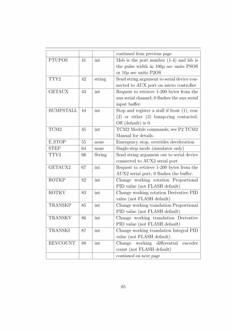
Appendix A AmigOS Command Set 83

Appendix B Initial File 87

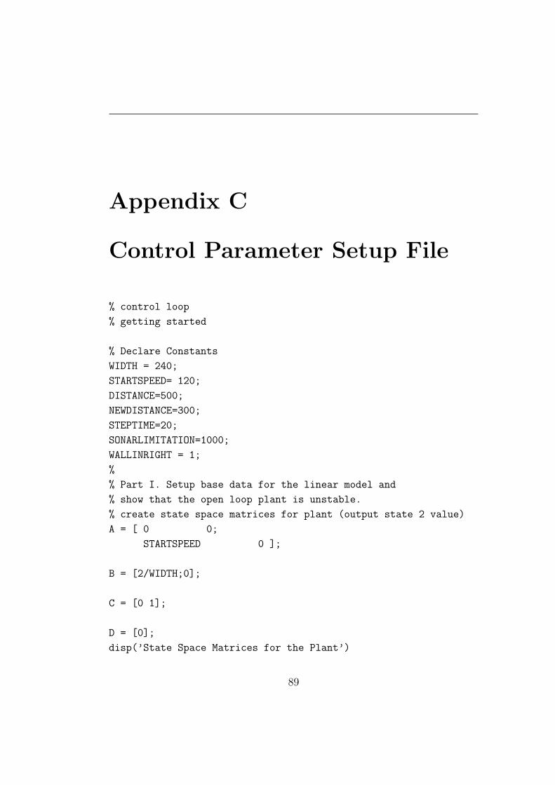
Appendix C Control Parameter Setup File 89

Bibliography 92

v

CONTENTS

Index 93

Vita 95

vi

LIST OF TABLES

List of Tables

2.1 Main Elements of AmigOS Communication Packet Protocol . 15

2.2 AmigOS Communication Packet Data Types . . . . . . . . . . 15

2.3 Standard AmigOS Server Information Packet (SIP) . . . . . . 18

2.4 AmigOS Client Command Packet . . . . . . . . . . . . . . . . 19

3.1 Synchronization Test Case 1 . . . . . . . . . . . . . . . . . . . 24




3.5 AmigOS Wheel Speed Analysis (mm/sec) . . . . . . . . . . . . 52

A.1 AmigOS Command Set . . . . . . . . . . . . . . . . . . . . . . 86

vii

LIST OF FIGURES

List of Figures

2.1 Real-Time Workshop Code Generation Process . . . . . . . . 9

2.2 Hardware Connection between Target PC and Host PC . . . 11

2.3 Configuration of Target Boot Disk . . . . . . . . . . . . . . . 12

2.4 xPC Target Boots, the Kernel and Display Information on the

Target PC . . . . . . . . . . . . . . . . . . . . . . . . . . . . 12

2.5 Loading a MATLAB Simulink Model to xPC Target . . . . . . 13

2.6 AmigoBot’s Physical Characteristics. . . . . . . . . . . . . . . 13

2.7 AmigoBot’s Client-server Architecture . . . . . . . . . . . . . 14

2.8 Hardware Connection between Target PC and AmigoBot . . . 20

2.9 The AmigoBot Communication Block . . . . . . . . . . . . . 21

3.1 Flow Chart of How to Start The AmigoBot . . . . . . . . . . 28

3.2 AmigoBot Connector . . . . . . . . . . . . . . . . . . . . . . 29

3.3 Second Level of the AmigoBot Connector. . . . . . . . . . . . 31

3.4 Synchronization & Initialization. . . . . . . . . . . . . . . . . . 33

3.5 The RS232 Received Buffer on the Target PC . . . . . . . . . 34

3.6 Sending the SYNC0 Packet . . . . . . . . . . . . . . . . . . . 35

3.7 Receiving the Echo of SYNC0 . . . . . . . . . . . . . . . . . 35

3.8 Receiving the Echo of SYNC1 . . . . . . . . . . . . . . . . . 36

3.9 Subsystem Receiving SIP . . . . . . . . . . . . . . . . . . . . . 37

3.10 Sub Subsystem Receiving SIP . . . . . . . . . . . . . . . . . . 38

3.11 Decoding the SIP to User Wanted Data . . . . . . . . . . . . . 41

3.12 Sub Subsystem to Detect the Speed of the Left Wheel . . . . . 41

3.13 Sub Subsystem Get the Sonar Values: New Sonar Readings

SonarRangeA and SonarRangeB . . . . . . . . . . . . . . . . . 43

3.14 Generating a Setting Wheel Speed Command Packet . . . . . 44

3.15 Five Examples of the Speed Commands . . . . . . . . . . . . . 45

viii

LIST OF FIGURES

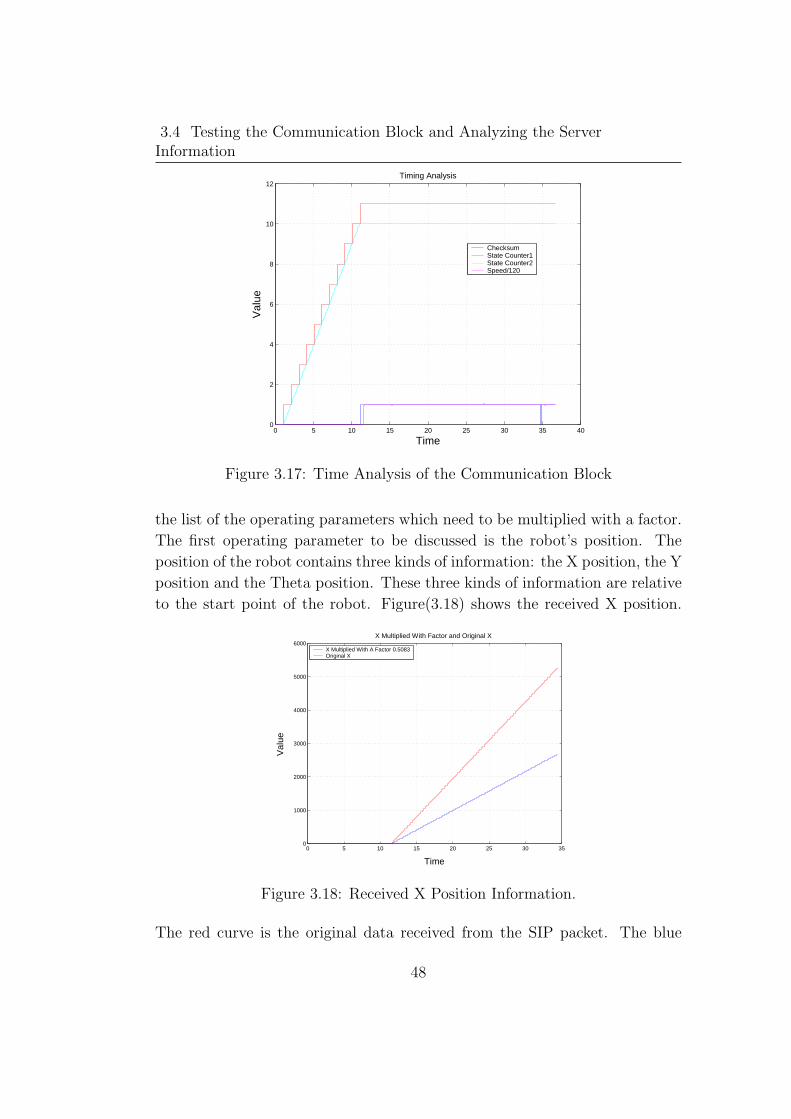
3.16 Timing Sequence Diagram of the Communication Block. . . . 47

3.17 Time Analysis of the Communication Block . . . . . . . . . . 48

3.18 Received X Position Information. . . . . . . . . . . . . . . . . 48

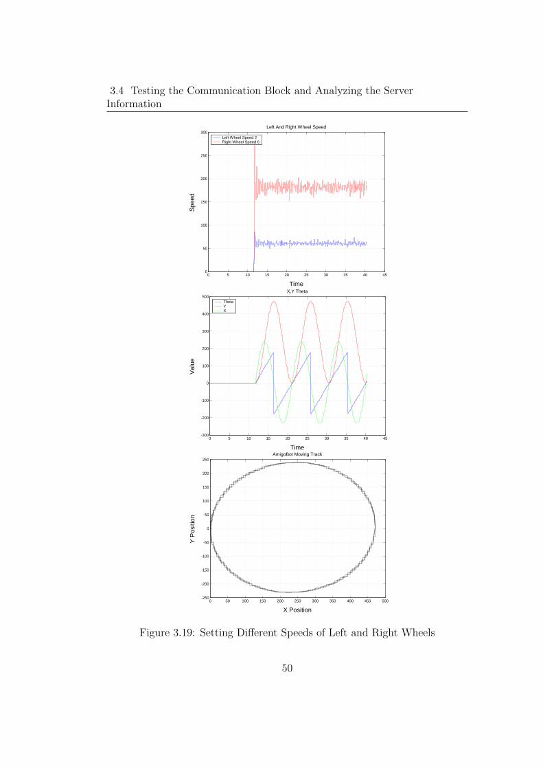
3.19 Setting Different Speeds of Left and Right Wheels . . . . . . . 50

3.20 Analyzing the Received Wheel Speed. . . . . . . . . . . . . . . 51

3.21 Received Left Wheel Speed with 7 Steps. . . . . . . . . . . . . 51

3.22 Received X Position Information (Wheel Speed with 6 Steps). 52

3.23 Find The Maximum Speed. . . . . . . . . . . . . . . . . . . . 53

3.24 Set the Left and Right Wheel Speed to Positive and Negative

Values . . . . . . . . . . . . . . . . . . . . . . . . . . . . . . . 53

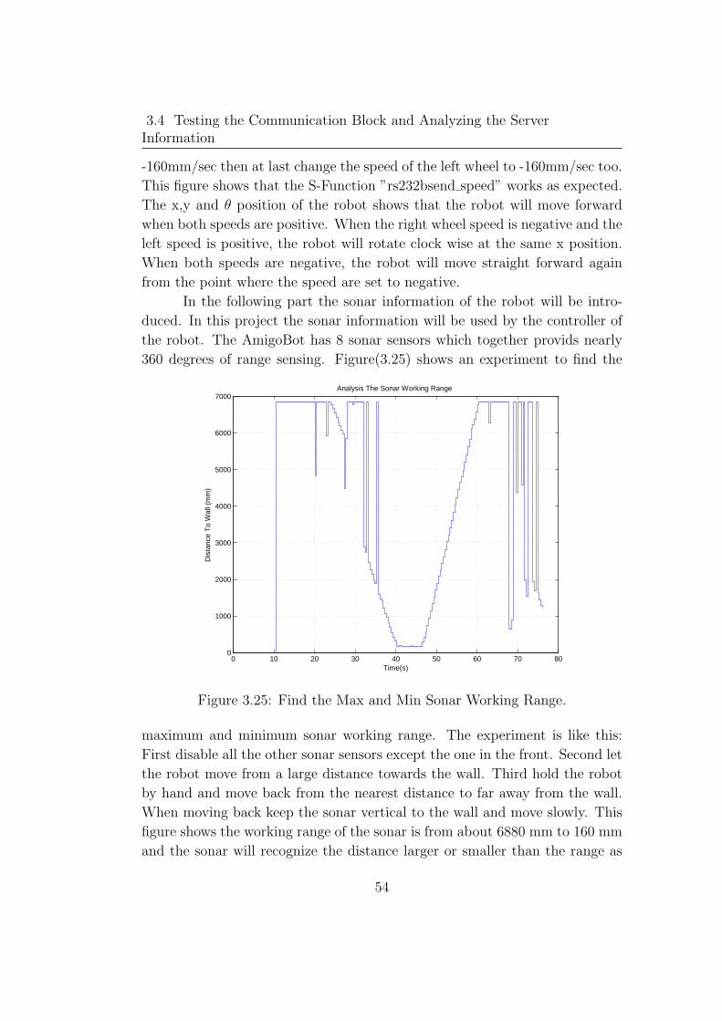
3.25 Find the Max and Min Sonar Working Range. . . . . . . . . . 54

3.26 Experiment To Test the Behavior of the Sonar 5 . . . . . . . . 55

3.27 Experimental Results of Rotating the Sonar 5 . . . . . . . . . 56

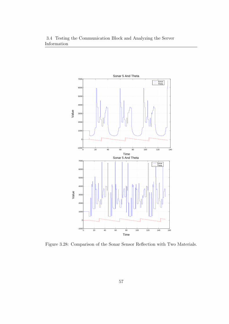
3.28 Comparison of the Sonar Sensor Reflection with Two Materials. 57

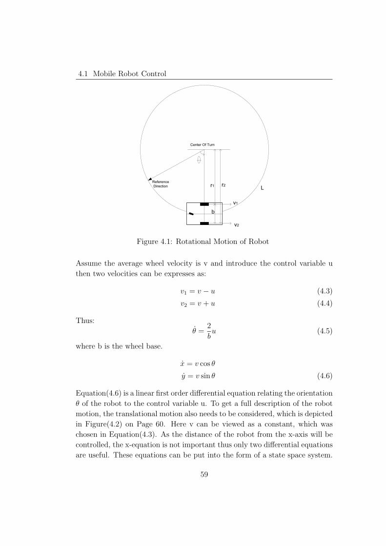
4.1 Rotational Motion of Robot . . . . . . . . . . . . . . . . . . . 59

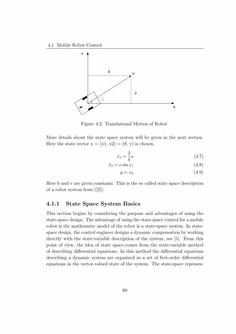
4.2 Translational Motion of Robot . . . . . . . . . . . . . . . . . 60

4.3 A State Variable Control System . . . . . . . . . . . . . . . . 61

4.4 Non-linearized Mathematic Model of The AmigoBot. . . . . . 62

4.5 Linearized and Non-linearized Model of the Open loop Control

of the AmigoBot . . . . . . . . . . . . . . . . . . . . . . . . . 63

4.6 Standard Control Loop for the Mobile Robot. . . . . . . . . . 63

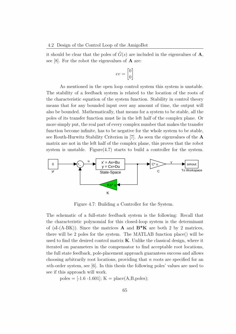
4.7 Building a Controller for the System. . . . . . . . . . . . . . 65

4.8 Linear Simulation Results. . . . . . . . . . . . . . . . . . . . 66

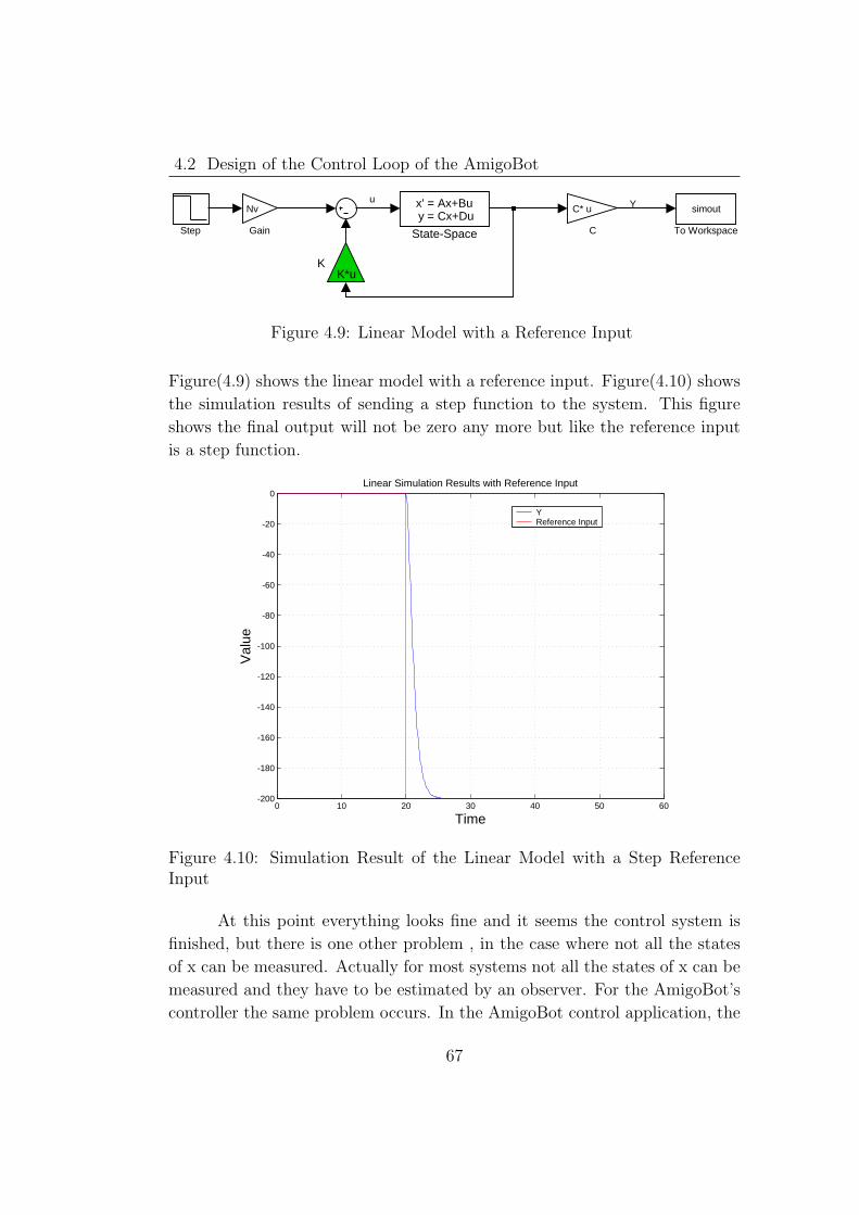
4.9 Linear Model with a Reference Input . . . . . . . . . . . . . . 67

4.10 Simulation Result of the Linear Model with a Step Reference

Input . . . . . . . . . . . . . . . . . . . . . . . . . . . . . . . 67

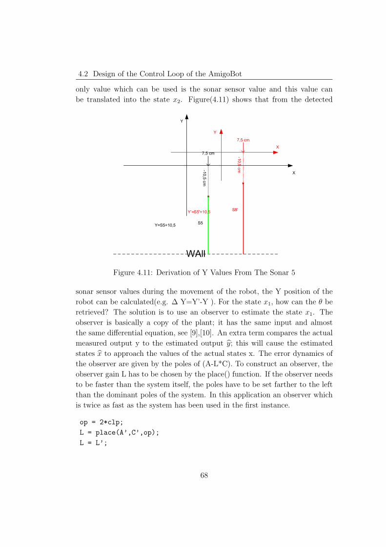
4.11 Derivation of Y Values From The Sonar 5 . . . . . . . . . . . 68

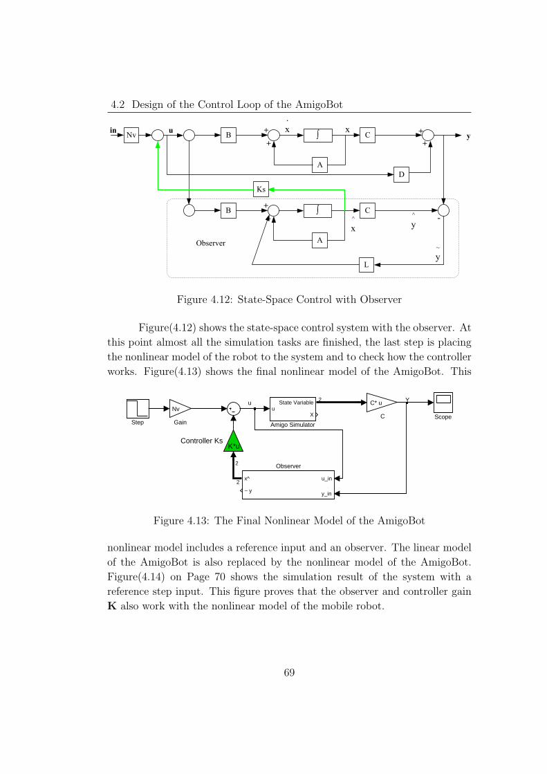
4.12 State-Space Control with Observer . . . . . . . . . . . . . . . 69

4.13 The Final Nonlinear Model of the AmigoBot . . . . . . . . . . 69

4.14 Simulation Result of Sending a Reference Step Function to the

Final Nonlinear Model of the AmigoBot . . . . . . . . . . . . 70

4.15 The Top Level of the AmigoBot’s Final Control System . . . . 70

4.16 Subsystem Observer and Controller . . . . . . . . . . . . . . . 71

4.17 Sub Subsystem Observer . . . . . . . . . . . . . . . . . . . . . 71

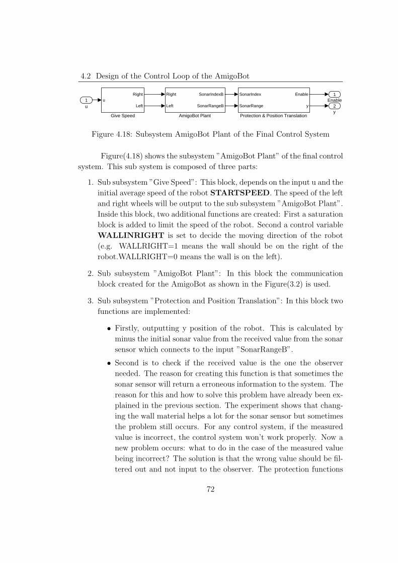
4.18 Subsystem AmigoBot Plant of the Final Control System . . . 72

ix

LIST OF FIGURES

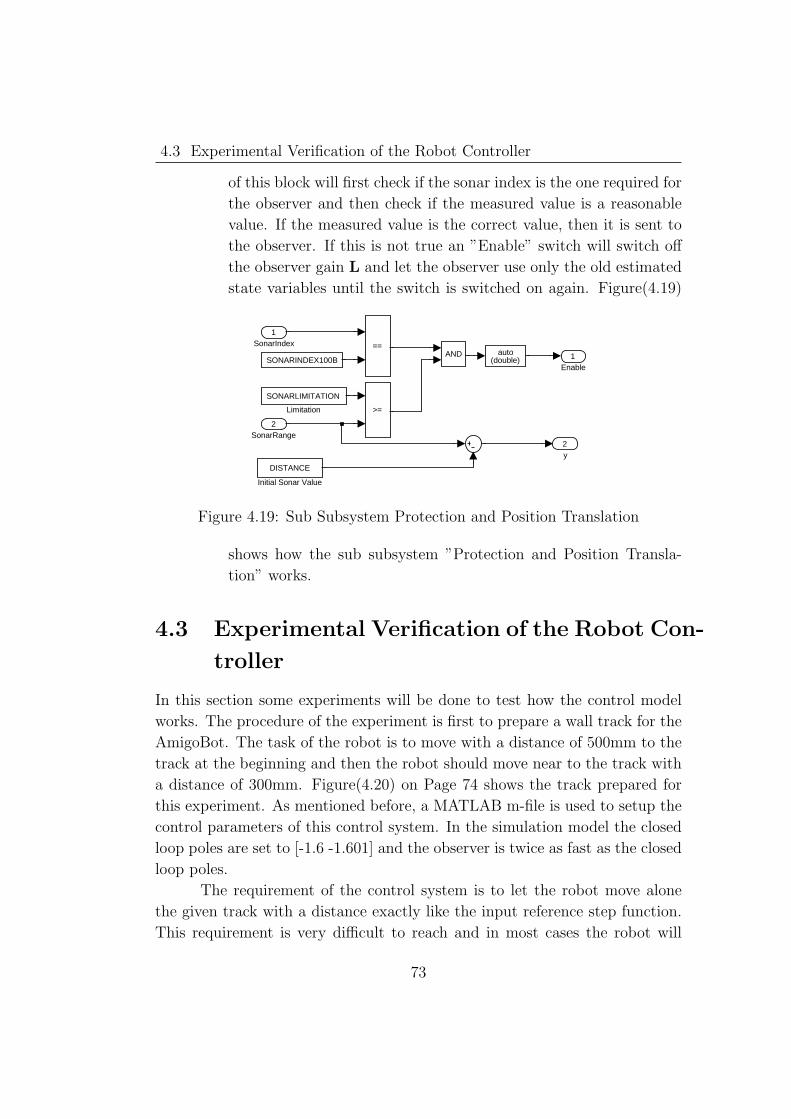
4.19 Sub Subsystem Protection and Position Translation . . . . . . 73

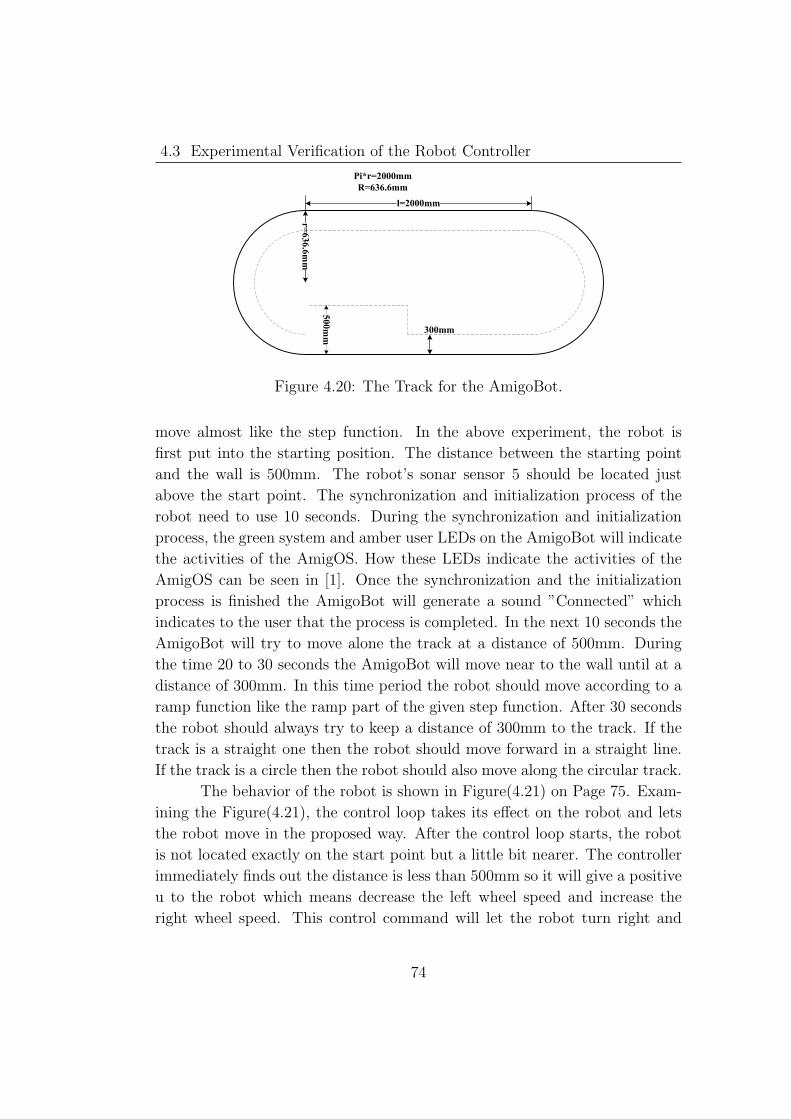
4.20 The Track for the AmigoBot. . . . . . . . . . . . . . . . . . . 74

4.21 Experiment A: The Received Sonar,Theta,U and the Given In-

put Information. . . . . . . . . . . . . . . . . . . . . . . . . . 75

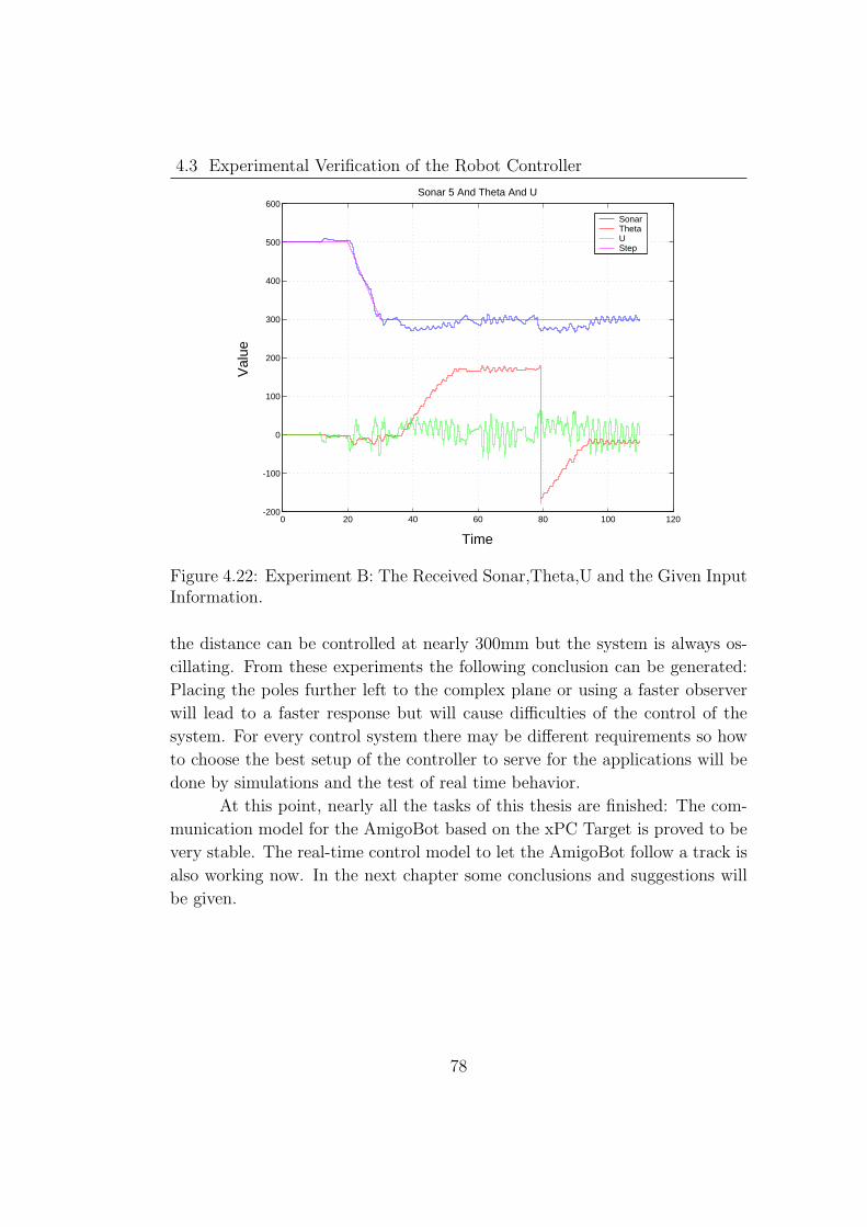
4.22 Experiment B: The Received Sonar,Theta,U and the Given In-

put Information. . . . . . . . . . . . . . . . . . . . . . . . . . 78

4.23 Experiment C: The Received Sonar,Theta,U and the Given In-

put Information. . . . . . . . . . . . . . . . . . . . . . . . . . 79

x

Chapter 1

Introduction

This thesis is based on a research work in the Automatic Control Laboratory

at the Department of Electrical Engineering and Computer Science of the

University of Applied Sciences Hamburg. In the laboratory some mobile robots

are used in student courses and research works. These robots have their own

software and control package. On the other hand, the software tool MATLAB

is the primary software used in the department for communication and control

because of its advantages. Therefore it is a very interesting research topic to

develop an interface to drive the robots by using MATLAB.

There are two possibilities to implement this interface. The simplest

approach is to use the basic software (ARIA) from the robot’s provider (Ac-

tivMedia). This solution is only possible in the MATLAB simulation mode

and was investigated in another thesis, see [12]. The drawbacks of this method

are possibly the inaccurate timing and the dependency of the windows oper-

ating system. Because of these drawbacks, the second possibility comes with

the idea of implementing a real-time interface for the robot. The xPC Target

from the MATLAB family provides a small and simple real time kernel to re-

alize this interface. This interface will be used later for the automatic control

laboratory.

1.1 Problem Overview

In order to find the real-time behavior of the interface, a real-time control

application for the mobile robot by using MATLAB will be included in the

thesis. This real-time control application will control a mobile robot moving

1


along a wall at a given distance. The track of the wall can be a straight one or

a curved one. The given distance can be set as a constant or as a mathematic

function (e.g. a step function).

One of the most important tasks for this thesis is to find out the func-

tionalities provided by the MATLAB for a real-time control system. MATLAB

is a high level, standard and widely spread software. It is a high-performance

language for technical computing. The Simulink, Real-Time Workshop and

xPC Target from the MATLAB family will be used in this thesis too, as they

are very powerful in building a real-time control system. The Simulink is a

software package used to model, simulate, and analyze systems whose outputs

change over time. The Real-Time Workshop is an extension of capabilities

found in Simulink and MATLAB to enable rapid prototyping of real-time

software applications on a variety of systems. The xPC Target is a solution

for prototyping, testing, and deploying real-time systems using standard PC

hardware. All these products from the MATLAB family are commonly used

to realize a real-time control application whose behavior is changed over time.

They are spread in almost every university, company and research center, so

in this thesis they are used to implement this real-time control application.

The final product of this thesis will be a Simulink block diagram running on

the xPC Target.

To realize this real-time control application a mobile robot and a real-

time environment are required for this project.

For the mobile robot the three-wheeled mobile robot AmigoBot from

ActivMedia was chosen in this application. AmigoBot is a small, 2 driven

wheels, differential drive and intelligent mobile robot. The AmigoBot drive

and sensor systems are powered and processed from a single controller, driven

by a high-performance, I/O-rich 20-MHz Hitachi H8 microprocessor. The

AmigoBot micro controller comes loaded with AmigOS operating system soft-

ware that manages all the low-level systems and electronics of the mobile robot.

It can be connected externally with RS232 serial link or wireless modem. The

AmigoBot comes standard with a single array of eight sonar sensors. The

sonar positions are fixed: one on each side, four facing forward, and two at the

rear, together providing nearly 360 degrees of range sensing. The sonar firing

rate is 20 Hz (50 milliseconds per sonar) and sensitivity ranges from 10cm (6

inches) to more than 5 meters (16 feet). The tasks of the AmigoBot in this

application are data acquisition and following the client’s control command,

2


once a connection between the client and the AmigoBot is established. The

AmigOS will send the position information of the robot back to the client and

waits for the client’s commands. The position information of the robot comes

from the feed back information of different sensors. One of the most important

pieces of feed back information is the distance from the wall. This informa-

tion is detected by one of the sonar sensors just above the right wheel. The

AmigoBot has its own communication protocol so the communication block

works on the client has to follow the communication protocol of the AmigoBot.

The xPC Target from the MATLAB is chosen to support the real-time

environment. It is an environment that uses a target PC, separate from a host

PC, for running real-time applications. This environment includes a host PC

and a target PC. The host PC is a development platform which has Visual

C++, MATLAB Simulink and Real-Time Workshop. The target PC is just a

normal PC which can be booted with an xPC boot disk. xPC Target does not

require DOS, Windows, Linux, or any another operating system on the target

PC. Instead, the target PC is booted with a boot disk that includes the highly

optimized xPC Target kernel. It is created on the host PC by setting up the

xPC Target environment properties for example the xPC Target kernel specific

for either serial or network communication. To create a target application, a

Simulink model will be created at first. xPC Target then uses the Simulink

model, Real-Time Workshop, and a third-party compiler to create the target

application on the host PC. Real-Time Workshop provides the utilities to

convert the Simulink models into C code and then with a third-party C/C++

compiler, compile the code into a real-time executable. This executable is then

converted to an image suitable for xPC Target and uploaded to the target PC.

The task of the xPC Target in this application is to design a control system

for the robot by constructing a Simulink block diagram. This block diagram

will be uploaded to the target PC from the host PC. After the running of

the application, the target PC will communicate with the AmigoBot via a

wireless modem. The block diagram on the target PC will analyze the received

information from the robot and send new commands to the robot in order to

control it.

The implementation of this application is divided into two parts. The

first part of the application is to build a communication block in a Simulink

diagram. By using this Simulink block diagram the xPC Target can commu-

nicate with the AmigoBot in real-time. Here the communication means the

3


xPC Target will establish a connection with the AmigoBot and through this

connection the application running on the target PC can receive information

from the robot and send control commands to the robot. The received infor-

mation will be sent to the control block and a new client command will be

generated. The content of the new client command depends on the result of

analyzing the received information. In this part the most important thing to

do is to establish a connection between the xPC Target and robot by following

the communication protocol of the AmigoBot. This part can be divided into

three steps:

1. The aim of the first step is to synchronize the connection and initialize

the robot. The synchronization is realized by sending and receiving some

synchronization packets. The initialization is done by sending initializa-

tion packets to the robot.

2. In the second step, the received information from the AmigoBot will be

decoded into categories.

3. The task of the third step is to send the client commands to the AmigoBot.

Problems occurring in this part are how to build the synchronization process,

how to decode the information from the robot and how to send different com-

mands to the robot. These problems will be solved by different solutions which

will be introduced during the implementation.

The second part of the application is to find a control method which

can control the robot moving along the wall with a given distance. This part

can be divided into two steps:

1. At first a mathematical description of the robot will be created and ana-

lyzed. From the mathematical view, the two driven wheeled robot can be

seen as a state-space system so the state-space control method is chosen

for this application. When using the state-space system to describe the

robot, there are only two state variables: the vertical position and the

angular position of the robot. Here the vertical and angular positions

described in a 2D plane are the y position and θ position. The horizontal

position of the robot is not of interest in this application. The two state

variables are needed by the controller to generate feed back information

to the robot. The feed back information is actually the speed at which

4

1.2 Organization of the Thesis

the two wheels should be set. In this step the first task is to find how to

get these two state variables. The distance from the robot to the wall

is the only information which can be used in this application. It can be

converted to the y position of the robot. It is detected by one of the

sonar sensors on the robot. Anther state variable θ can’t be established

directly but it can be recovered by using an observer.

2. After the mathematical behavior of the robot is clear, the second task

in this part is to build a simulator to simulate the behavior of the robot.

By using this simulator the reasonable control parameters can be found

out to let the robot move along the wall in real time. In this application

there are two problems which affect the control system:

• The sonar’s sensitivity is influenced by the robot’s position and

the material of the wall. The sonar sensor uses an ultrasonic wave

which reflects back from the wall to measure the distance from the

wall. If the sonar sensor has a large angle with the wall then there

may be no waves reflected back to the sensor which will result in a

wrong feed back information. This problem will be solved by using

a better material which can reflect the ultrasonic waves to every

direction. The details of the solution will be introduced later.

• The sonar value will only be refreshed every 400 milliseconds by

default. As the control block used in this application is a feed

back control system, the information coming from the robot is very

important. A feed back rate of 400 milliseconds is not sufficient. To

solve this problem a new sonar polling sequence is set to let only

one sonar sensor working all the time. This will lead the sonar value

to be refreshed every 100 milliseconds. How to realize this will be

explained in the following sections.

In the following chapters, how to realize this application and solutions to the

problems will be explained in detail.


This thesis is broken up into parts according to the main steps taken in the

realization of the real-time control system of a mobile robot: The next four

5


chapters detail the design process, the hardware, the software and the resulting

problems.

• Chapter 2 outlines the design issue of the communication block of this

application. The design issue includes which hardware and software

are used in this project, and reasons for them. The interface of the

communication block.

• Chapter 3 starts with the implementation of the communication block.

In this chapter lots of experiments are used to analyze the behavior

of the AmigoBot. By working with these experiments some changes are

added to the project design which is mentioned in Chapter 2. During the

implementation some new problems and the problems listed in Chapter

2 are solved by the final model. In the last part of Chapter 3 some tests

are used to demonstrate how the communication block works.

• Chapter 4 opens with the design of the control block. The mathematical

background of this control system will be given in the beginning of the

chapter. The simulation of the control block and the main factors which

will influence the control system will be shown too. At the end of this

chapter the implementation of the control system with some experiments

will be introduced.

• Chapter 5 summarizes the contributions of this thesis and poses sugges-

tions and goals for future work.

• The appendices to this thesis give detailed information on specific topics

related to the work presented. Appendix A is the table AmigOS Com-

mand Set. Appendices B and C are some initial MATLAB m file used

in the project.

6

Chapter 2

Design of the AmigoBot’s

Communication Interface

In this section the design procedure of the communication model for the real-

time control system will be introduced. The design procedure starts from

choosing the software and hardware. After this the interface of the commu-

nication model will be given. In the following sections more details about

the design procedure will be explained. As mentioned in the introduction,

the hardware used in this application is the AmigoBot and xPCTarget(Host

and Target PC). The software used in this application is the AmigOS and the

MATLAB xPC Target software set.

2.1 The xPC Target

The title of this thesis shows this is a real-time control application. Currently,

most control applications are based on PC control and the use of the Windows

operating system. In this application the Windows operating system will only

be used on the host PC. The reason is that it is not an exact real-time operating

system and is expensive. For educational purpose and real-time requirements

of this application, the xPC Target is used to realize this control task. The

xPC Target is a solution for prototyping, testing, and deploying real-time

systems using standard PC hardware. It is an environment which uses a target

PC, separate from a host PC, for running real-time applications. Changing

parameters in the target application while it is running in real time, and

checking the results by viewing signal data, are two important prototyping

7

2.1 The xPC Target

tasks. xPC Target includes a command-line and graphical user interfaces to

complete these tasks.

2.1.1 Host and Target PC

The working procedure of the xPC Target is first to develop a real-time ap-

plication on the host PC. This application is built by creating a MATLAB

model file which uses the Simulink libraries. The model file will be compiled

as a real-time executable and then uploaded to the target PC. The target PC

will provide a real-time environment for the application. The application can

be started or stopped from the target PC or the host PC. Both the target and

host PC can control the application when it is running. For example the pa-

rameters of the application can be changed from the host or target PC during

the run time. The xPC Target hardware requires a host PC and a target PC.

The target PC only needs to have the I/O boards supported by xPC Target

and a boot disk. More details about the software on the host PC and target

PC and how they work together will be introduced in the following sections.

2.1.2 xPC Target Software Set

xPC Target is a PC-compatible product which is installed on a host computer

running a Microsoft Windows operating system. xPC Target requires the

following products from MathWorks:

• MATLAB – Control and interaction with the xPC Target software en-

vironment and target application using a command-line interface.

• Simulink – Model dynamic physical systems and controllers using block

diagrams.

• Real-Time Workshop – Convert Simulink blocks and Stateflow charts

into C code.

• C Compiler – Use a third-party C compiler and Real-Time Workshop to

build a target application. The C compiler can be a Microsoft Visual

C/C++ compiler (version 5.0, 6.0, or 7.0) or a Watcom C/C++ compiler

(version 10.6 or 11.0) or other supported compilers.

8

2.1 The xPC Target

• xPC Target Embedded Option – deploys stand-alone target applications

and custom GUI applications that communicate with the target appli-

cation. Note that custom GUI applications can be created without the

xPC Target Embedded Options.

The MATLAB ,Simulink and C Compiler are common softwares used in every

university, they will not be detailed in this thesis. The xPC Target Embed-

ded Option will not be used in this application. The only thing need to be

mentioned is the Real-Time Workshop and MATLAB S-Functions (system-

functions).

Real-Time Workshop is an extension of capabilities of Simulink and

MATLAB that automatically generates, packages and compiles source code

from Simulink models to create real-time software applications on a variety

of systems. Real-Time Workshop provides the utilities to convert a Simulink

models into C code and then, with a third-party C/C++ compiler, compile

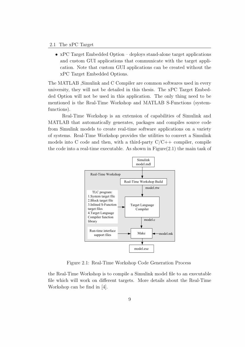
the code into a real-time executable. As shown in Figure(2.1) the main task of

Simulink

model.mdl

Real-Time Workshop Build

Target Language

Compiler

Make

model.exe

Real-Time Workshop

model.rtw

TLC program:

1.System target file

2.Block target file

3.Inlined S-Function

target files

4.Target Language

Compiler function

library

Run-time interface

support files

model.c

model.mk

Figure 2.1: Real-Time Workshop Code Generation Process

the Real-Time Workshop is to compile a Simulink model file to an executable

file which will work on different targets. More details about the Real-Time

Workshop can be find in [4].

9

2.1 The xPC Target

S-Functions (system-functions) provide a powerful mechanism for ex-

tending the capabilities of Simulink. The most common use of S-Functions is

to create custom Simulink blocks. It can be used for a variety of applications,

including:

• Adding new general purpose blocks to Simulink

• Adding blocks that represent hardware device drivers

• Incorporating existing C code into a simulation

• Describing a system as a set of mathematical equations

• Using graphical animations

An advantage of using S-Functions is that it can be used to build a general

purpose block that can be used many times in a model, varying parameters

with each instance of the block. In this application the S-Functions work

together with the Real-Time Workshop to solve various kinds of problems.

These problems include:

• Extending the set of algorithms (blocks) provided by Simulink and Real-

Time Workshop

• Interfacing existing (hand-written) C-code with Simulink and Real-Time

Workshop

• Generating highly optimized C-code for embedded systems

The explanation of S-Function above means that the S-Function is a tool which

allows let’s the developer to create their own MATLAB tool block for their

special applications. More details about the S-Function and why they are used

in this application will be introduced in Chapter 3.

2.1.3 Downloading A Model to the Target PC

In this section a simple introduction about how the xPC Target works will be

given. The first step is to build a connection between the host PC and the

target PC. There are two ways to connect them: one is the serial communi-

cation(e.g serial RS232) and the other is using network communication. Here

the network communication is used to connect the target and the host PC

because it has two advantages:

10

2.1 The xPC Target

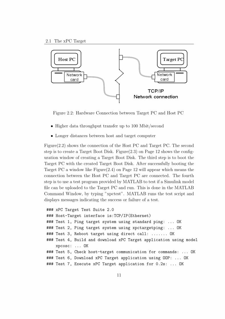
Figure 2.2: Hardware Connection between Target PC and Host PC

• Higher data throughput transfer up to 100 Mbit/second

• Longer distances between host and target computer

Figure(2.2) shows the connection of the Host PC and Target PC. The second

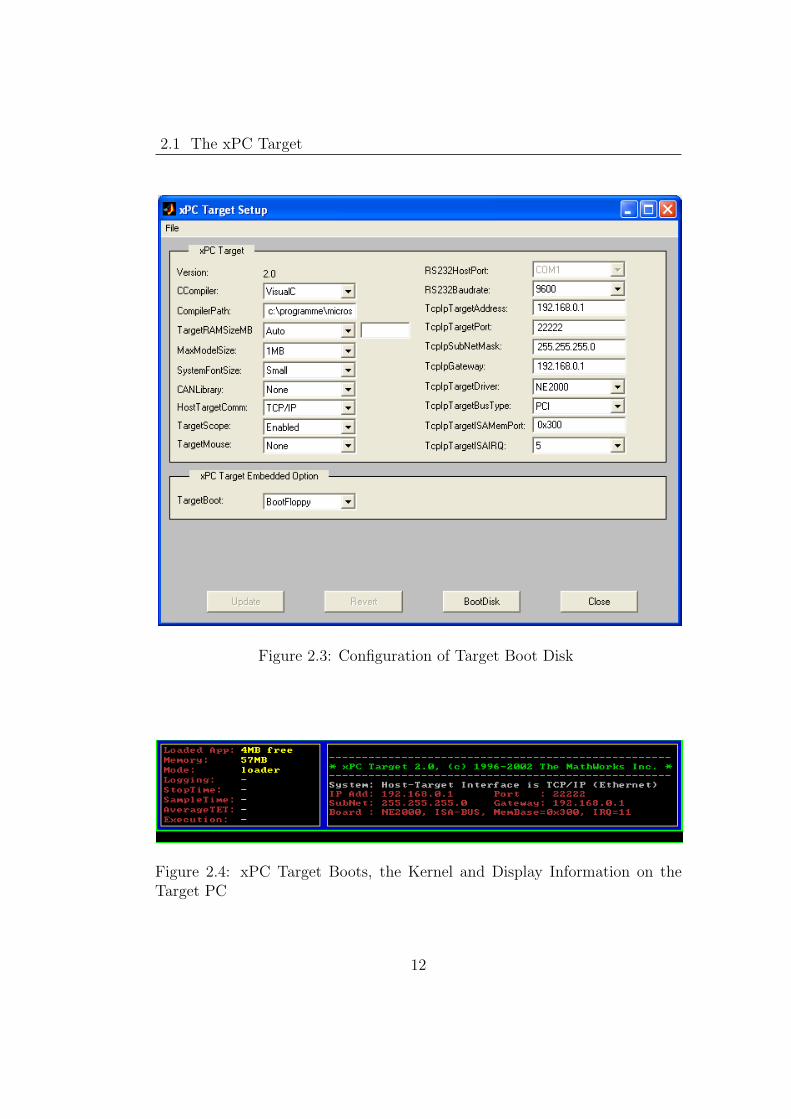
step is to create a Target Boot Disk. Figure(2.3) on Page 12 shows the config-

uration window of creating a Target Boot Disk. The third step is to boot the

Target PC with the created Target Boot Disk. After successfully booting the

Target PC a window like Figure(2.4) on Page 12 will appear which means the

connection between the Host PC and Target PC are connected. The fourth

step is to use a test program provided by MATLAB to test if a Simulink model

file can be uploaded to the Target PC and run. This is done in the MATLAB

Command Window, by typing ”xpctest”. MATLAB runs the test script and

displays messages indicating the success or failure of a test.

### xPC Target Test Suite 2.0

### Host-Target interface is:TCP/IP(Ethernet)

### Test 1, Ping target system using standard ping: ... OK

### Test 2, Ping target system using xpctargetping: ... OK

### Test 3, Reboot target using direct call: ....... OK

### Test 4, Build and download xPC Target application using model

xpcosc: ... OK

### Test 5, Check host-target communication for commands: ... OK

### Test 6, Download xPC Target application using OOP: ... OK

### Test 7, Execute xPC Target application for 0.2s: ... OK

11

2.1 The xPC Target

Figure 2.3: Configuration of Target Boot Disk

Figure 2.4: xPC Target Boots, the Kernel and Display Information on theTarget PC

12

2.2 The AmigoBot

Figure 2.5: Loading a MATLAB Simulink Model to xPC Target

### Test 8, Upload logged data and compare it with

simulation: ... OK

### Test Suite successfully finished

The above message shows that the xPC Target is successfully connected. As

seen in Figure(2.5), the name of the model, the size of the model, the sam-

ple rate of the model and the status of the model are displayed in the xPC

Target’s information window. More information about the xPC Target can be

found in [3] and also will be introduced in the following chapters during the

implementation of this application.

2.2 The AmigoBot

As described, the object to be controlled in this application is a mobile robot

called AmigoBot. The reasons for using the AmigoBot is that it is a commonly

used robot for educational purposes. The advantage of the AmigoBot and

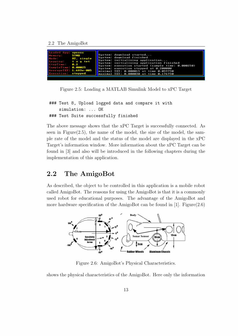
more hardware specification of the AmigoBot can be found in [1]. Figure(2.6)

Sonar Sensor

28cm

33cm

Body

Figure 2.6: AmigoBot’s Physical Characteristics.

shows the physical characteristics of the AmigoBot. Here only the information

13

2.2 The AmigoBot

Client Application

Server Information Commands

Communication Packets

Velocity &Angle

ControlsPosition

Integration

Sonar & I/O

Schedules

PWM

Control

Encoder

Counting

Sonar

Ranging

I/O

Control

Server Informaiotn

Robot Specific Functions

Figure 2.7: AmigoBot’s Client-server Architecture

about the AmigoBot’s communication protocol and the sonar sensors will be

explained. The AmigoBot uses an intelligent client/server control architecture

developed by Dr. Kurt Konolige. In the model, the server works to manage all

the low-level details of the mobile robot’s systems. These include operating the

motors, firing the sonar, collecting sonar and motor encoder data, and so on.

The client application sends commands to the server and receives the returned

report from the server. Figure(2.7) shows the client-server architecture of the

AmigoBot. As described in the introduction the whole application is divided

into two steps: the communication model and the control model. Before

starting the design of the communication model and the control model, the

communication with AmigoBot via the AmigOS client-server interface will be

described.

2.2.1 Communication Packet Protocol

AmigOS communicates with a client application by using special packet proto-

cols: command packets from client to server, and Server Information Packets

14

2.2 The AmigoBot

(SIPs) from server to client. Both are byte data streams consisting of four main

elements: a two-byte header, a one-byte count of the number of command/data

bytes, the client command and its arguments or the server information data,

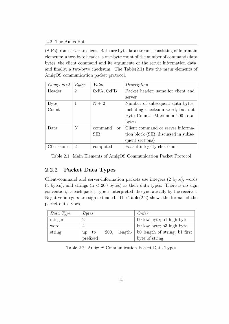
and finally, a two-byte checksum. The Table(2.1) lists the main elements of

AmigOS communication packet protocol.

Component Bytes Value Description

Header 2 0xFA, 0xFB Packet header; same for client and

server

Byte

Count

1 N + 2 Number of subsequent data bytes,

including checksum word, but not

Byte Count. Maximum 200 total

bytes.

Data N command or

SIB

Client command or server informa-

tion block (SIB; discussed in subse-

quent sections)

Checksum 2 computed Packet integrity checksum

Table 2.1: Main Elements of AmigOS Communication Packet Protocol

2.2.2 Packet Data Types

Client-command and server-information packets use integers (2 byte), words

(4 bytes), and strings (n < 200 bytes) as their data types. There is no sign

convention, as each packet type is interpreted idiosyncratically by the receiver.

Negative integers are sign-extended. The Table(2.2) shows the format of the

packet data types.

Data Type Bytes Order

integer 2 b0 low byte; b1 high byte

word 4 b0 low byte; b3 high byte

string up to 200, length-

prefixed

b0 length of string; b1 first

byte of string

Table 2.2: AmigOS Communication Packet Data Types

15

2.2 The AmigoBot

2.2.3 Packet Checksum

The checksum is used in almost every communication to check if there is

disturbance. The AmigOS communication protocol contains the checksum

too. It is calculated by successively adding data byte pairs (high byte first) to

the running checksum (initially zero), disregarding sign and overflow. If there

is an odd number of data bytes, the last byte is XORed to the low-order byte

of the checksum. Using the MATLAB existing tool block to calculate this

checksum for the robot is too complicated. An S-Function will be created to

calculate the checksum of the received block and compare it with the received

checksum to see if the received packet is wrong.

2.2.4 Packet Errors

Currently, AmigOS ignores a client command packet whose byte count exceeds

200 or has an erroneous checksum. The client should similarly ignore erroneous

server information packets. AmigOS does not acknowledge receipt of a com-

mand packet nor does it have any facility to handle client acknowledgment of

a server information packet.

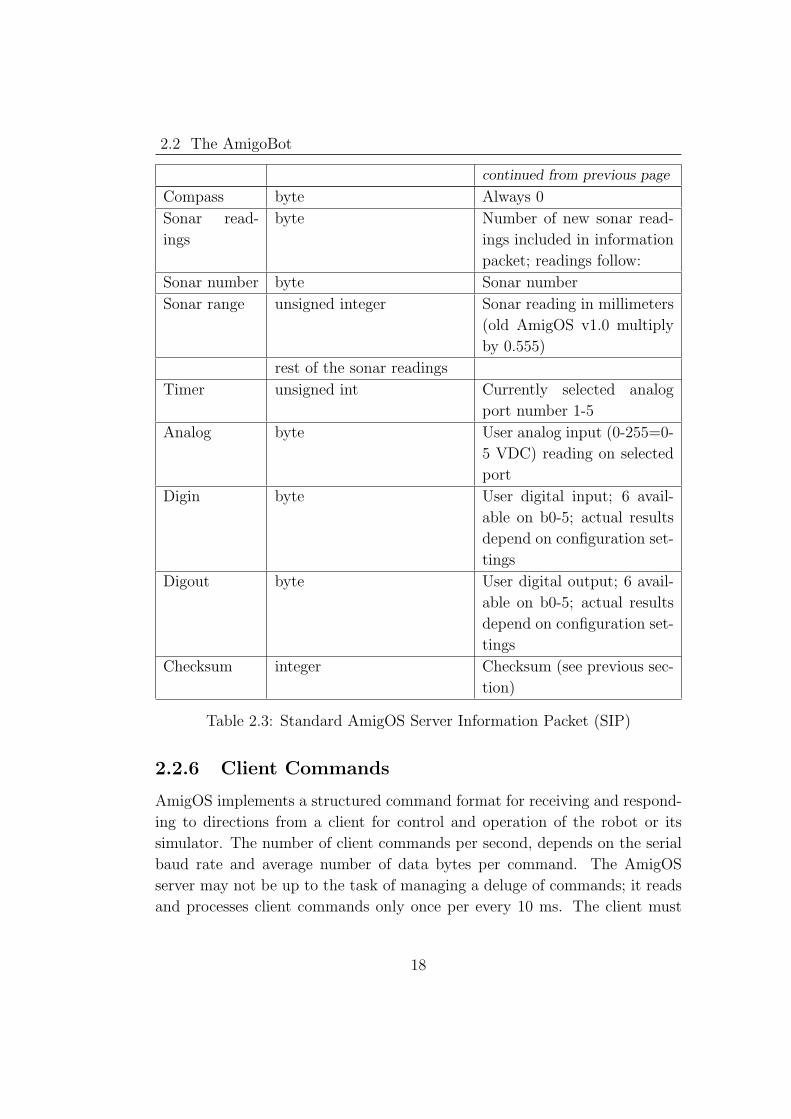
2.2.5 Server Information Packets

Once connected, AmigOS automatically sends a packet of information back

to the client every 100 milliseconds, depending on the infoCycle setting in the

robot FLASH parameters. The standard AmigOS Server Information Packet

(SIP) informs the client about a number of the robot’s operating parameters

and readings, using the orders and data types shown in the Table(2.1) on

Page 15. AmigOS also supports several additional server information packet

types, including an alternative server information packet. Table(2.3) shows

the list of the format of SIP.

Name Data Type Description

Header integer Exactly 0xFA, 0xFB

Byte Count byte Number of data bytes + 2 <

201 (0xC9) max.

continued on next page

16

2.2 The AmigoBot

continued from previous page

Status byte = 0x3S; where S = Motors status

sfSTATUSSTOPPED (2) Motors moving

sfSTATUSMOVING (3) Motors stopped

Xpos unsigned integer (15 ls-bits) Wheel-encoder integrated

coordinates; platform-

dependent units; multiply

by 0.5083 to convert to

millimeters

Ypos unsigned integer (15 ls-bits)

Th pos signed integer Orientation in platform-

dependent units multiply by

0.001534 for degrees.

L vel signed integer Wheel velocities (respective

Left and Right) in platform-

dependent units;

R vel signed integer multiply by 0.6154 to con-

vert to mm/sec

Battery byte Battery charge times 10

volts

Bumpers integer Motor stall indicators. Bit 0

of the lsbyte is the left wheel

stall indicator = 1 if stalled;

bit 0 of the msbyte is the

right wheel stall.

Control signed integer Setpoint of the server’s an-

gular position multiply by

0.001534 for degrees

PTU unsigned integer bit 0 reflects motors engaged

state (1 of engaged) and bit

1 reflects the sonar toggle (1

if on)


17

2.2 The AmigoBot


Compass byte Always 0

Sonar read-

ings

byte Number of new sonar read-

ings included in information

packet; readings follow:

Sonar number byte Sonar number

Sonar range unsigned integer Sonar reading in millimeters

(old AmigOS v1.0 multiply

by 0.555)

rest of the sonar readings

Timer unsigned int Currently selected analog

port number 1-5

Analog byte User analog input (0-255=0-

5 VDC) reading on selected

port

Digin byte User digital input; 6 avail-

able on b0-5; actual results

depend on configuration set-

tings

Digout byte User digital output; 6 avail-

able on b0-5; actual results

depend on configuration set-

tings

Checksum integer Checksum (see previous sec-

tion)

Table 2.3: Standard AmigOS Server Information Packet (SIP)

2.2.6 Client Commands

AmigOS implements a structured command format for receiving and respond-

ing to directions from a client for control and operation of the robot or its

simulator. The number of client commands per second, depends on the serial

baud rate and average number of data bytes per command. The AmigOS

server may not be up to the task of managing a deluge of commands; it reads

and processes client commands only once per every 10 ms. The client must

18

2.2 The AmigoBot

send a command at least once every two seconds or so;otherwise, the com-

munication watchdog server will stop the robot’s onboard drives. Table(2.4)

shows the format of the client commands.

Component Bytes Value Description

Header 2 0xFA, 0xFB Packet header; same for client

and server

Byte Count 1 N + 2 Number of subsequent command

bytes plus checksum, not includ-

ing Byte Count. Maximum of

200 bytes.

Command

Number

1 0 - 255 Client command number;

Argument

Type (com-

mand depen-

dent)

1 0x3B or 0x1B

or 0x2B

Required data type of com-

mand argument: positive integer

(sfARGINT), negative integer or

absolute value (sfARGNINT), or

string (sfARGSTR)

Argument

(command

dependent)

n data Command argument; integer or

string

Checksum 2 computed Packet integrity checksum

Table 2.4: AmigOS Client Command Packet

The AmigOS command is comprised of a one-byte command number option-

ally followed by, if required by the command, a one-byte description of the

argument type and the two (integers) or more (strings) byte argument value.

The number of client commands per second, depends on the Control serial

baud rate, average number of data bytes per command, synchronicity of the

communication link, and so on. AmigOS command processor runs on a ten

millisecond interrupt cycle, but the server response speed depends on the com-

mand. Typically, client commands are limited to a maximum of one every 20

milliseconds.

19

2.3 Connection between the xPC Target and AmigoBot

2.2.7 Client Command Argument Types

There are three different types of AmigOS client-command arguments: pos-

itive integers two bytes long, negative integers two bytes long, and NULL-

terminated strings consisting of as many as 196 characters. The byte order is

least-significant byte first. Negative integers are transmitted as their absolute

value, unlike information packets, which use sign extension for negative inte-

gers; see below. The argument is an integer, a string, or nothing, depending

on the command.

2.3 Connection between the xPC Target and

AmigoBot

The AmigoBot AmigOS servers require a serial communication link to a client.

The serial link may be:

• A tether (AmigoLEASH) from the Control serial connector on the top

of AmigoBot to a base station computer

• An optional radio modem pair—one inside AmigoBot and its companion

connected to the serial port of the client PC.

Target PC Radio ModemRS232 AmigoBot With aRadio ModemFigure 2.8: Hardware Connection between Target PC and AmigoBot

In this project the radio modem link is chosen, because the radio modem is

more flexible than the serial link. As shown in Figure(2.8), the connection

between the Target PC and AmigoBot.

20

2.4 The AmigoBot Communication Block

2.4 The AmigoBot Communication Block

After the above introduction the next step is to build an interface for the

AmigoBot communication block. The Figure(2.9) shows the AmigoBot com-

AmigoBot Communication

Block

Check Sum

LeftWheel

RightWheel

Theta

Y

X

SonarReading

SonarIndex

SonarRange

Start

Left Wheel Speed

Right Wheel Speed

Figure 2.9: The AmigoBot Communication Block

munication block. This communication block is prepared for building a control

system of the robot. For the robot control system the main control variables

are the speeds of the wheels so the communication block must have the speed

inputs. As introduced previously the state variable of the state-space system

comes from the sonar sensor so the outputs must have sonar sensor value.

In order to help the user to find more useful information, more detailed po-

sitional information will be output too. This interface has three inputs and

several outputs. The input ”Start” is used to control the start and stop of the

application. The inputs ”Left Wheel Speed” and ”Right Wheel Speed” are

used to set the wheel speeds of the robot. The outputs of the communication

block are used to output the decoded information from the received SIP(e.g

the position information of the robot).

21

Chapter 3

Implementation of the

AmigoBot Communication

System

The first step to work with the AmigoBot is to establish a connection with the

AmigoBot. There are lots of different communication interfaces which can be

used for the AmigoBot like the Aria software or self built interfaces. In this

project the MATLAB Real-Time Work Shop and xPC Target are chosen as

the development tools and the communication will be realized by a MATLAB

model file. Before exerting any control, a client application must first establish

a connection to the AmigoBot server. Over that established communication

link, the client then sends commands to and receives operating information

from the server. In the following parts, details of this model file are given.

3.1 Analyzing the Synchronization and Ini-

tialization Process

3.1.1 Analyzing the Synchronization Process

When first started, the AmigoBot is in a ”wait” state; AmigOS listens for

communication packets over its designated port. To establish a connection, the

client application must send a series of three synchronization packets through

the host’s communication port: SYNC0, SYNC1 and SYNC2. At the same

22

3.1 Analyzing the Synchronization and Initialization Process

time the client has to retrieve the server responses.

The synchronization sequence of bytes are (in hexadecimal notation):

SYNC0: 0xFA, 0xFB, 0x03, 0x00, 0x00, 0x00

SYNC1: 0xFA, 0xFB, 0x03, 0x01, 0x00, 0x01

SYNC2: 0xFA, 0xFB, 0x03, 0x02, 0x00, 0x02

AmigOS responds to each client command, forming a succession of identical

synchronization packets. The client should listen for the returned packets

and only issue the next synchronization packet after it has received the echo.

In order to test the behavior of the AmigoBot synchronization procedure an

experiment is done with a software called LookRS232 which can send and

receive the data from the COM port by using the RS232 connections.

Time(s) Sent Data (hex) Received Data (hex)

0023.704 FA FB 03 00 00 00

0023.782 FA FB 03 00 00 00

0024.047 FA FB 03 01 00 01

0024.125 FA FB 03 01 00 01

0024.360 FA FB 03 02 00 02

0024.438 FA FB 1D 02 48 61 6D 62

0024.454 75 72 67 5F 33 33 31 00

0024.469 50 69 6F 6E 65 65 72 00

0024.469 41 6D 69 67 6F 00 DD A4

0024.657 FA FB 03 01 00 01

0024.829 FA FB 21 32 00 00 00 00

0024.829 00 00 00 00 00 00 6E 00

0024.844 00 00 00 02 00 00 02 00

0024.844 50 03 01 20 0B 01 00 00

0024.860 00 00 58 CC

0024.922 FA FB 21 32 00 00 00 00

0024.938 00 00 00 00 00 00 6D 00

0024.938 00 00 00 02 00 00 02 02

0024.954 D5 12 03 35 03 01 00 00


23



0024.954 00 00 7F 4A

0025.032 FA FB 21 32 00 00 00 00

0025.032 00 00 00 00 00 00 6D 00

0025.047 00 00 00 02 00 00 02 04

0025.047 8F 06 05 DC 05 01 00 00

0025.063 00 00 1C 08

Table 3.1: Synchronization Test Case 1


0023.704 FA FB 03 00 00 00

0023.782 FA FB 00

0024.047 FA FB 03 01 00 01

0024.125 FA FB 03 01 00 01

0024.360 FA FB 03 02 00 02

0024.438 FA FB 1D 02 48 61 6D 62

0024.454 75 72 67 5F 33 33 31 00

0024.469 50 69 6F 6E 65 65 72 00

0024.469 41 6D 69 67 6F 00 DD A4



0006.880 6D 69 67 6F 00 DD A4

0006.890 FA FB 03 00 00 00

0006.890 FA FB 03 FF 00 FF

0006.906 FA FB 03 00 00 00

0006.906 FA FB 03 00 00 00

0006.922 FA FB 03 01 00 01

0006.922 FA FB 03 01 00 01

0007.222 FA FB 03 02 00 02

0007.222 FA FB 03 02 00 02


24



0006.890 FA FB 03 00 00 00

0006.890 FA FB 03 01 00 01

0006.906 FA FB 03 02 00 02

0006.906 FA FB 03 01 00 01

0006.922 FA FB 06 04 3B 01 00 05 3B

0006.922 FA FB 03 00 00 00

0006.922 FA FB 03 02 00 02

0007.000 FA FB 03 00 00 00 FA FB

0007.000 03 FF 00 FF FA FB 03 FF

0007.015 00 FF FA FB 03 FF 00 FF

0007.031 FA FB 03 FF 00 FF


The above four tables demonstrate four different cases of the synchro-

nization process. In the following section these four cases will be explained.

The Table(3.1) on Page 23 shows a case, in which a successful synchronization

is completed. This table shows that the client sends the three synchronization

packet one by one and with an interval of about 0.3 seconds. The client also

receives three identical synchronization packets just after each packets is sent.

The Table(3.1) shows that as introduced in [1], once connected the AmigBot

will automatically send the SIPs back to the client every 100 milliseconds.

This means the receive block of the client needs to operate at least with the

same rate.

The Table(3.2) on Page 24 and Table(3.3) on Page 24 illustrate some

strange behavior of the AmigoBot. From the specification, if a SYNC0 packet

is sent by the client, the server should respond with an identical echo packet.

The client should then receive a packet like ”0xFA 0xFB 0x03 0x00 0x00 0x00”

but the Table(3.2) shows that a ”0xFA 0xFB 0x00” packet will be received.

The situation of Table(3.2) happens every time when the AmigoBot is switched

on. After several tests it was proven, that this behavior is a result only of

switching on the AmigoBot. The second erroneous behavior pattern is shown

in Table(3.3). Sometimes when the AmigoBot is switched on, at first the client

will receive a strange packet. There are two reasons for this: The first reason is

that the client’s RS232 buffer keeps the old data from the last connection. The

second reason is that the AmigoBot still sends the rest of data of the packet

25


which belongs to the last connection, because the AmigoBot is suddenly shut

down before the whole packet is sent. This second behavior pattern leads to a

synchronization error. If a SYNC0 packet is sent during the synchronization

phase, an identical echo packet will be received on the client side. If any packet

is sent at the wrong time, the AmigoBot will recognize that a wrong packet

is received and send back a packet ”0xFA 0xFB 0x03 0xFF 0x00 0xFF” to

the client. The packet ”0xFA 0xFB 0x03 0xFF 0x00 0xFF” is always used to

notify the client that some errors occurred during the communication. Because

of this behavior the client should send the SYNC0 packet again in order to

build the synchronization as shown in Table(3.3).

Table (3.4) on Page 24 shows an unsuccessful synchronization. The

reason is that the client sends the command with a higher rate than the

AmigoBot’s maximum accepted rate. The AmigoBot reads and processes the

client commands only once every 10 ms. If the client sends the commands

faster than this, the AmigoBot will send back an error message ”0xFA 0xFB

0x03 0xFF 0x00 0xFF”. After these four tests, the behavior of the AmigoBot

during the synchronization phase is clear. In the next section the initialization

process will be explained.

3.1.2 Analyzing the Initialization Process

3.1.2.1 Opening the Servers–OPEN

Once a communication link is established, the client should then send the

OPEN command #1 (no argument; 0xFA, 0xFB, 0x03, 0x01, 0x00, 0x01)

which causes the AmigoBot to perform a few housekeeping functions, start its

sonar and motor controllers (among other things), listen for client commands,

and begin transmitting server information packets.

3.1.2.2 Set the Sonar Firing Sequence–POLLING

When connected and opened, the AmigOS sonar server begins firing AmigoBot’s

sonar in the predefined default sequence, clockwise, beginning with the sonar

closest to the left wheel (sonar #0). As discussed in the introduction the

firing rate of the sonar sensor is 20Hz. If using the default sequence, each

sonar sensor will fire every 400 milliseconds which is too long for the control

requirement. To solve this problem a new sequence has to be set by sending

26


the POLLING command #3 (string argument,only sonar #0 works; 0xFA,

0xFB, 0x0C, 0x03, 0x2B, 0x01, 0x01, 0x01, 0x01, 0x01 0x01, 0x01,0x01, 0x07,

0x2F) to the AmigoBot. In order to activate the new sequence at the begin-

ning, this command has to be sent before the OPEN command is sent.

3.1.2.3 Enable the Motor

Once the client is connected to the AmigoBot , the AmigoBot’s motors are

disabled, regardless of their state when last connected. There are two ways

to start the motor: First is to manually press the black MOTORS/TEST

button. Second is to send an ENABLE client command #4 with an integer

argument of 1 ”0xFA 0xFB 0x06 0x04 0x3B 0x01 0x00 0x05 0x3B”. In this

project the second way will be used. Now the process of the synchronization

and initialization is clear, the next step is starting to build the AmigoBot

communication block.

3.1.3 Building the Synchronization and Initialization

Model

In the previous two sections the analyzing work was done and the next step

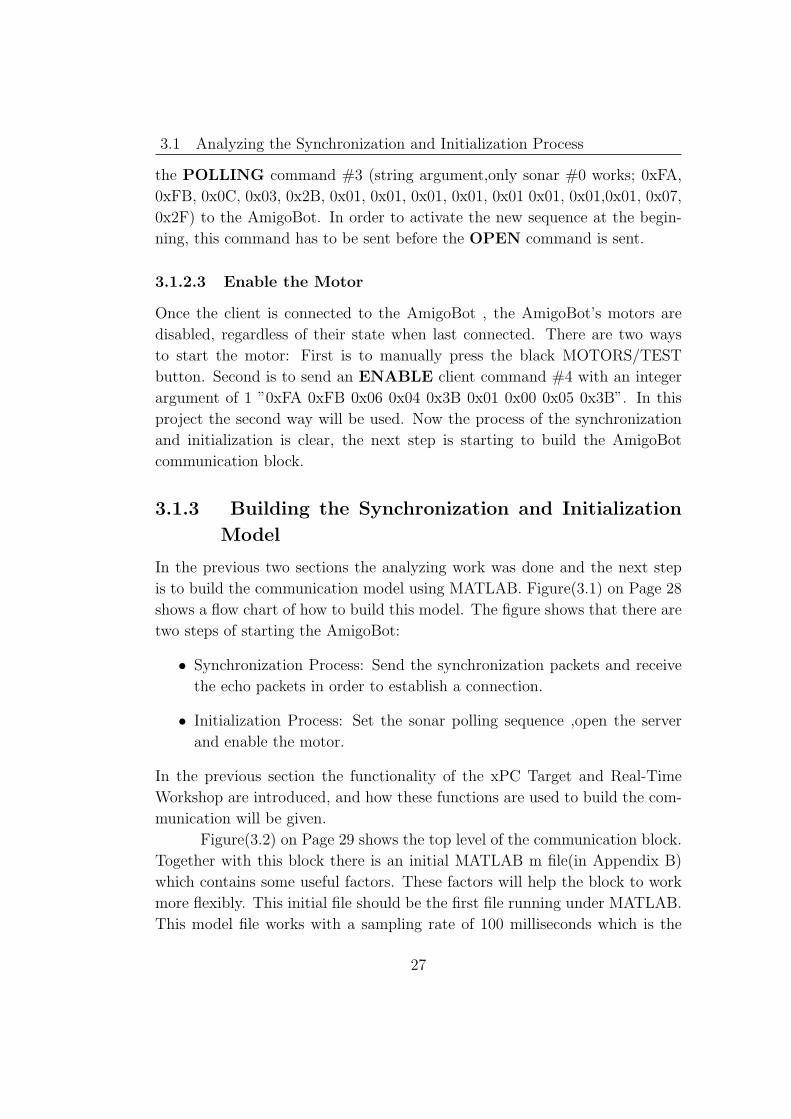
is to build the communication model using MATLAB. Figure(3.1) on Page 28

shows a flow chart of how to build this model. The figure shows that there are

two steps of starting the AmigoBot:

• Synchronization Process: Send the synchronization packets and receive

the echo packets in order to establish a connection.

• Initialization Process: Set the sonar polling sequence ,open the server

and enable the motor.

In the previous section the functionality of the xPC Target and Real-Time

Workshop are introduced, and how these functions are used to build the com-

munication will be given.

Figure(3.2) on Page 29 shows the top level of the communication block.

Together with this block there is an initial MATLAB m file(in Appendix B)

which contains some useful factors. These factors will help the block to work

more flexibly. This initial file should be the first file running under MATLAB.

This model file works with a sampling rate of 100 milliseconds which is the

27


Send SYNC0

Receive 3 Bytes Echo SYNC0

Received=FA FB 03

Clear the Received Buffer of the Target PC

Received=FF 00 FF

YES


YES

Send SYNC0

NO

Do Nothing

Received=FA FB 00

YES

Do Nothing

NO

Send SYNC0

NO

Send SYNC1


Send SYNC2

Received=FA FB XX

YESNO

Do NothingReceive XX Bytes Echo SYNC1 or SYNC0


Set Sonar POLLING Sequence

Received=FA FB XX

YESNO

Do NothingReceive XX Bytes Echo SYNC1 or SYNC2

Send OPEN

Connect & Send ENABLE Motor

S

y

n

c

h

r

o

n

i

z

a

t

i

o

n

I

n

i

t

i

a

l

i

z

a

t

i

o

n

Figure 3.1: Flow Chart of How to Start The AmigoBot

28


Step Size: 0.1sPort: COM1Baud Rate:9600

11SonarRangeB

10 SonarIndexB

9SonarRangeA

8 SonarIndexA

7SonarReading

6X

5Y1

4Th

3RightWheel

2LeftWheel

1Check Sum

1

Start

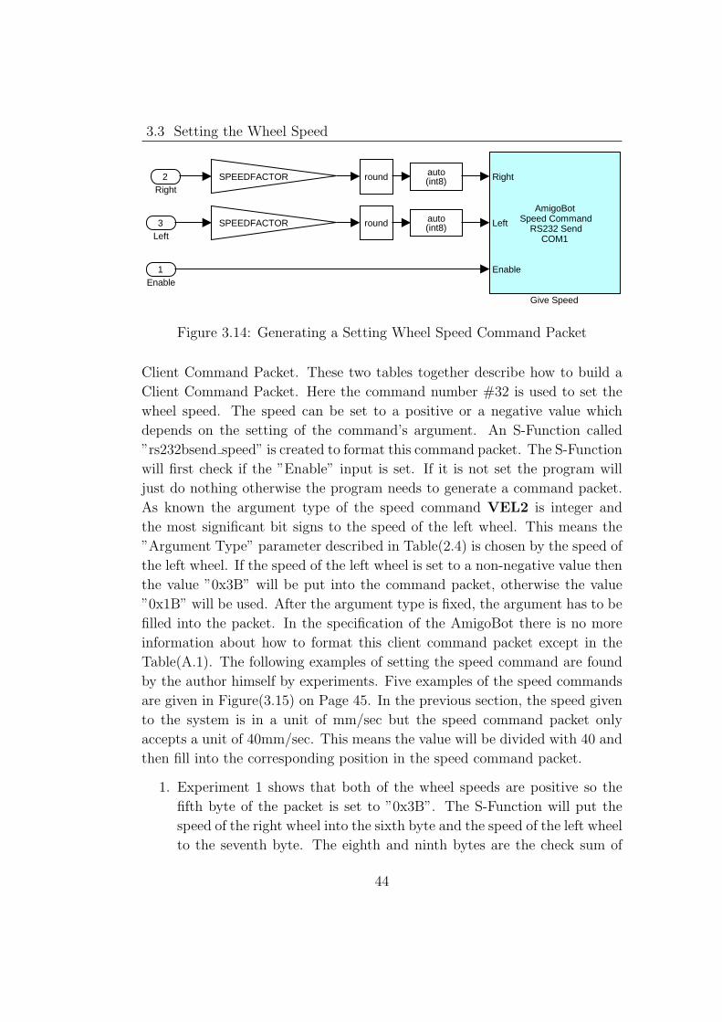
RS-232Mainboard

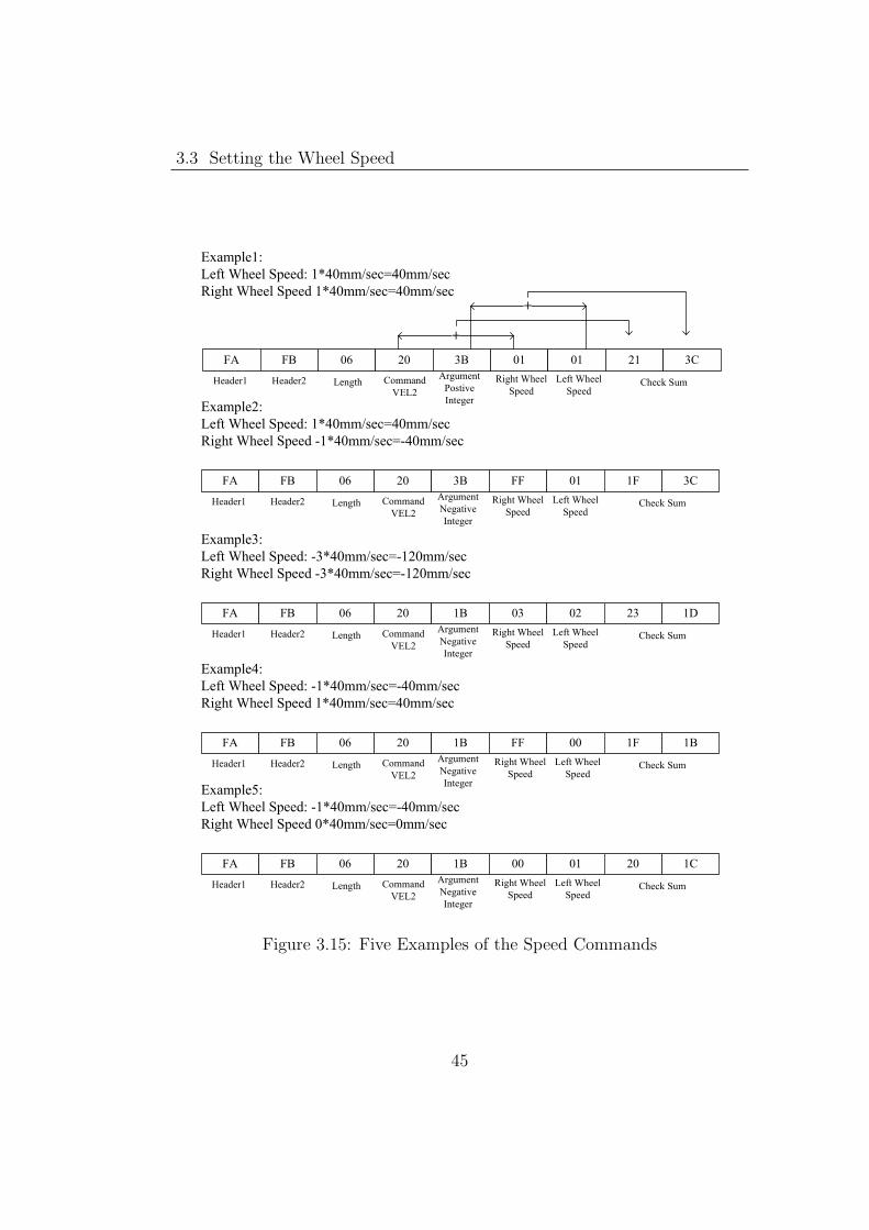
Setup

RS232

160

R

240

L

Start

RightWheelSpeed

LeftWheelSpeed

Check Sum

Left

Right

Th

Y

X

SonarReading

SonarIndexA

SonarRangeA

SonarIndexB

SonarRangeB

AmigoBot Plant

Figure 3.2: AmigoBot Connector

same as the transmission rate of the SIPs. At the top level there is one ”RS-

232 Mainboard Setup” block, three inputs and eleven outputs. The ”RS-232

Mainboard Setup” block is used to initialize the communication of a COM1

port. The three inputs are used to:

1. Start: Start the AmigoBot with ”1” and disconnect the AmigoBot with

”0”.

2. Right: Set a speed to the right wheel of the AmigoBot with a unit of

mm/sec.

3. Left: Set a speed to the left wheel of the AmigoBot with a unit of

mm/sec.

The unit of speed can be changed by changing the speed factor SPEEDFAC-

TOR in the initial file. For example if the SPEEDFACTOR is set to 1, it

29


means the input speed multiplied by 40 will be the output speed in mm/sec.

The eleven outputs are the received values from the AmigoBot:

1. CheckSum: Represents the status of the current packet. ”1” means that

the current packet’s checksum is correct. ”0” means that the current

packet has been distorted during the transmission.

2. LeftWheel: The received left wheel speed.

3. RightWheel: The received right wheel speed.

4. Th: The received orientation position.

5. X: The received X position.

6. Y: The received Y position.

7. SonarReading: Number of new sonar sensor readings in the packet.

8. SonarIndexA: The even index of the sonar sensor number in the sonar

polling sequence.

9. SonarRangeA: The sonar range of the sonar sensor 0,2,4,6.

10. SonarIndexB: The odd index of the sonar sensor number in the sonar

polling sequence.

11. SonarRangeB: The sonar range of the sonar sensor 1,3,5,7.

As mentioned in Chapter 2 the AmigoBot will send the SIPs every 100 mil-

lisecond or 50 milliseconds depending on the configuration of the AmigOS. If

the configuration of the SIP is different, then the format of the SIP is also

different. In comparing the 100 millisecond configuration with the 50 millisec-

ond configuration, the sonar information can be different. The sonar firing

rate of the AmigoBot is every 50 milliseconds and the 8 sonar sensors will fire

one after the other. This means every 50 milliseconds only one sonar sensor

is working and all the others are sleeping.If the configuration is set to send

the SIPs every 100 milliseconds, then there will be two sonar sensors putting

their measured values in the SIP. By default the 8 sonar sensor values will be

sent in 4 continuous SIPs while the sonar sensors are firing in a continuous

sequence. If the SIPs are sent every 50 milliseconds then there will be only

30


one sonar measured value in the SIP. The 8 sonar sensor values will be sent

in 8 continuous SIPs. The AmigoBot Connecter shown above works only for

the situation in which the SIPs are sent every 100 milliseconds. This is the

default configuration of the robot and it can be changed to 50 milliseconds.

The default polling sequence of the sonar sensors is continuous and this can

be changed by using the POLLING command. The POLLING command

is used to set a new sonar sensor firing sequence(e.g only one sonar sensor

fires every 50 milliseconds). In this application only the sonar sensor #5 is of

interest, so in the initial file the factor SEQUENCE1 to SEQUENCE8 are

all set to 6 and the factor SonarIndex100B is set to 5. This means when

the application starts, the sonar sensor #5 will fire every 50 milliseconds and

the output SonarRangeB will output the received value of sonar sensor #5.

This is the solution to the problem mentioned in the introduction, now the

feed back information comes every 100 milliseconds not in every 400 millisec-

onds as before. Figure(3.3) shows the second level of the whole model. The

11SonarRangeB

10SonarIndexB

9SonarRangeA

8 SonarIndexA

7SonarReading

6X

5Y

4Th

3Right

2Left

1Check Sum

Start

Synchronization & Initialization

Enable

Right

Left

Set Speed

Received data

Left

Right

Th

Y

X

SonarReading

SonarIndexA

SonarRangeA

SonarIndexB

SonarRangeB

Decode SIP

auto(double)

Start

Check Sum

Data

Receive SIP

3LeftWheelSpeed

2RightWheelSpeed

1Start

Figure 3.3: Second Level of the AmigoBot Connector.

31


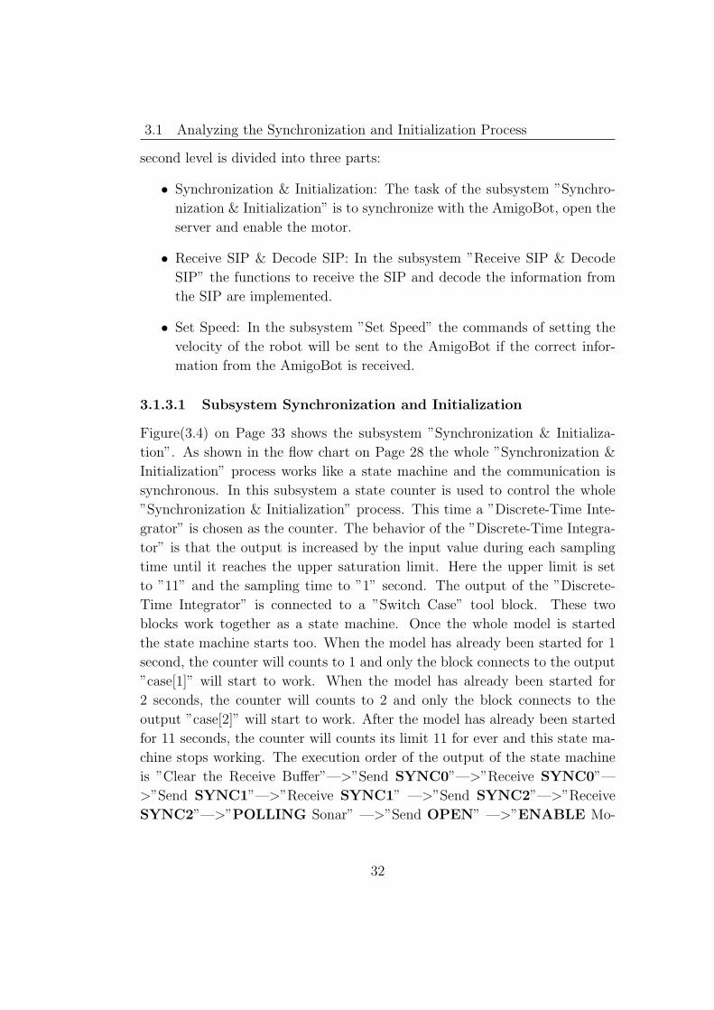
second level is divided into three parts:

• Synchronization & Initialization: The task of the subsystem ”Synchro-

nization & Initialization” is to synchronize with the AmigoBot, open the

server and enable the motor.

• Receive SIP & Decode SIP: In the subsystem ”Receive SIP & Decode

SIP” the functions to receive the SIP and decode the information from

the SIP are implemented.

• Set Speed: In the subsystem ”Set Speed” the commands of setting the

velocity of the robot will be sent to the AmigoBot if the correct infor-

mation from the AmigoBot is received.

3.1.3.1 Subsystem Synchronization and Initialization

Figure(3.4) on Page 33 shows the subsystem ”Synchronization & Initializa-

tion”. As shown in the flow chart on Page 28 the whole ”Synchronization &

Initialization” process works like a state machine and the communication is

synchronous. In this subsystem a state counter is used to control the whole

”Synchronization & Initialization” process. This time a ”Discrete-Time Inte-

grator” is chosen as the counter. The behavior of the ”Discrete-Time Integra-

tor” is that the output is increased by the input value during each sampling

time until it reaches the upper saturation limit. Here the upper limit is set

to ”11” and the sampling time to ”1” second. The output of the ”Discrete-

Time Integrator” is connected to a ”Switch Case” tool block. These two

blocks work together as a state machine. Once the whole model is started

the state machine starts too. When the model has already been started for 1

second, the counter will counts to 1 and only the block connects to the output

”case[1]” will start to work. When the model has already been started for

2 seconds, the counter will counts to 2 and only the block connects to the

output ”case[2]” will start to work. After the model has already been started

for 11 seconds, the counter will counts its limit 11 for ever and this state ma-

chine stops working. The execution order of the output of the state machine

is ”Clear the Receive Buffer”—>”Send SYNC0”—>”Receive SYNC0”—

>”Send SYNC1”—>”Receive SYNC1” —>”Send SYNC2”—>”Receive

SYNC2”—>”POLLING Sonar” —>”Send OPEN” —>”ENABLE Mo-

32


u1

case [ 1 ]:

case [ 2 ]:

case [ 3 ]:

case [ 4 ]:

case [ 5 ]:

case [ 6 ]:

case [ 7 ]:

case [ 8 ]:

case [ 9 ]:

case [ 10 ]:

case [ 13 ]:

State Machine

T

z-1

State Counter

case: { }

Send SYNC1

case: { }

Send SYNC0

case: { }

Send OPEN

case: { }

Send SYNC2

case: { }

Receive SYNC2

case: { }

Receive SYNC1

case: { }

Receive SYNC0

case: { }

Polling Sonar

NOT 2

case: { }

Enable Motor

case: { }

Disconnect

auto(double)

case: { }

Clear the Receive Buffer

1Start

Figure 3.4: Synchronization & Initialization.

33


tor”. If the input ”Start” changes to ”0” then the process ”Disconnect” will

be executed.

1. ”Clear the Receive Buffer”: In this state a built-in S-Function will clear

the RS232 received buffer on the Target PC. Figure(3.5) shows the RS232

Current Received Byte

Current Read Byte

Figure 3.5: The RS232 Received Buffer on the Target PC

buffering mechanism of the target PC. The buffer is a circular buffer with

a size of 1024 bytes. There are two pointers of the circular buffer: one

points to the current received byte from the AmigoBot, the other points

to the current read byte by the receive block. If the receiving speed is

much faster than the reading speed and once the differences are greater

than 1024 bytes, the old unread bytes will be wrapped up by the newly

received bytes. If the receiving speed is slower than the reading speed,

the receive block will wait until a new byte comes. Why the first state

is the ”Clear the Receive Buffer” is already explained in the previous

section for a case such as Table(3.3).

2. ”Send SYNC0”: In this state the SYNC0 packet will be sent. Figure(3.6)

on Page 35 shows the SYNC0 packet is sent by the ”RS232 Binary Send

Block”. The ”RS232 Binary Receive Block” is a tool block provided by

the Simulink Library for the xPC Target. In this state a 6 bytes long

packet ”0xFA 0xFB 0x03 0x00 0x00 0x00” will be sent to the AmigoBot

via the COM1 port of the Target PC with a sample rate inherited from

the upper block.

34


[250 251 3 0 0 0]

SYNC0

RS232 SendCOM1

RS232Binary Send

case: { }

Action Port

Figure 3.6: Sending the SYNC0 Packet

3. ”Receive SYNC0”: In this state the receiving process will follow the

flow chart given in the previous section. Figure(3.7) shows how this

UnpackUnpack

[250 251 3 0 0 0]

[250 251 3 0 0 0]

==

==

==

==

==

Data

Enable

RS232 SendCOM1

Data

Enable

RS232 SendCOM1

Length

Enable

Done

Data

RS232 ReceiveCOM1

Length

Enable

Done

Data

RS232 ReceiveCOM1

NOTOR

AND

3

Length

255

FF

251

FB

250

FA

(double)

(double)

auto(double)

3

0

1

3

case: { }

Figure 3.7: Receiving the Echo of SYNC0

receiving procedure works. The first step in this state is to receive 3

bytes. If the three bytes is ”0xFA 0xFB 0x00” this means the SYNC0

is received by the AmigoBot and the process will go to the next state.

If not the program will receive the next 3 bytes. The second step is to

check these 3 new bytes, if they are ”0x00 0x00 0x00” then the process

can go to the next state otherwise the SYNC0 has to be sent again.

4. ”Send SYNC1”: In this state the SYNC1 packet will be sent.

35


5. ”Receive SYNC1: In this state the echo of SYNC1 or the echo of the

SYNC0 packet will be received. Whether the echo of the SYNC1 or

SYNC0 will be received depends on the state ”Receive SYNC0”. If

in the state ”Received SYNC0” there is no packet SYNC0 sent, then

the echo of SYNC1 will be received in this state. Otherwise the echo of

SYNC0 will be received. Figure(3.8) shows how this receive procedure

Packet Length

Unpack==

==

Length

Enable

Done

Data

RS232 ReceiveCOM1

Length

Enable

Done

Data

RS232 ReceiveCOM1

AND

251

FB

250

FA

auto(double)

auto(double)

1

3

case: { }

Figure 3.8: Receiving the Echo of SYNC1

works. This procedure is a standard receiving block for the AmigoBot.

Firstly it receives the first three bytes of an AmigoBot communication

packet and finds out the length of the received packet. Second it config-

ures another receiving block to receive the rest data of the packet. This

procedure guarantees a whole packet is received when the length of the

packet is unknown.

6. ”Send SYNC2”: In this state the SYNC2 packet will be sent.

7. ”Receive SYNC2: In this state the echo of the SYNC2 or SYNC1

packet will be received.

8. ”POLLING Sonar: In this state a sonar sensor firing sequence will be

set to the AmigoBot’s sonar server. The sequence is defined in the initial

file and can be changed before each start of the application.

9. ”Send OPEN”: Before this state the synchronization process is finished

and the xPC Target should successfully be connected to the AmigoBot.

36

3.2 Receive and Decode the SIPs

Now the initialization process can be started. The first task of the ini-

tialization process is to send an OPEN command to the AmigoBot.

10. ”ENABLE Motor”: In this state the command ENABLE motor will

be sent and the motor of the AmigoBot will be started.

This is the implementation of the synchronization and the initialization subsys-

tems. When the synchronization and initialization are finished the AmigoBot

will start to send its SIPs to the client.


3.2.1 Subsystem Receive the SIPs

In the following part, the functionality of the subsystem ”Receive and De-

code the SIPs” will be introduced. Figure(3.9) shows the subsystem ”Receive

2Data

1Check Sum

u1 case [ 10 ]:T

z-1

State CounterRate Transition

auto(double)

case: { }

CheckSum

Data

1Start

Figure 3.9: Subsystem Receiving SIP

SIP”. In this subsystem a synchronous ”State Counter” is used. This ”State

Counter” works the same as the ”State Counter” on the subsystem ”Synchro-

nization and Initialization” and both of these two counters have the same

output value at the same time. The only difference is that before this ”State

Counter” a ”Rate Transition” tool block is used. This ”Rate Transition” will

convert the sample time of this block from 1 second to 0.1 second which means

the subsystem connecting to the output, works with a sampling time of 0.1

second too. The reason of using it is that the AmigoBot sends the SIP packets

with a rate of 0.1s and the client has to send the commands with a rate of 0.1s

also. this subsystem there is another subsystem which has two outputs. The

two outputs are the checksum and received data. This subsystem will start

37


to work only after the application has already been running for 10 seconds.

The reason is that the ”State Counter” will enable the subsystem connect to

it when the counter counts 10. Figure (3.10) shows the sub subsystem ”Re-

2Data

1CheckSum

Data

CheckSum

AmigoBot SIP RS232 Receive 8COM1

AmigoBot SIP Receive Block

case: { }

Action Port

Figure 3.10: Sub Subsystem Receiving SIP

ceive SIP”. In this sub subsystem there is only a receive block. The receive

block contains an S-Function called ”rs232brec amigo8”. This S-Function did

the most important job of the whole block. When this S-Function starts the

following situations may occur:

1. There is less than one SIP in the circular buffer.

2. There are several SIPs already in the circular buffer.

In the first step it will receive all the bytes from the target PC’s RS232 circular

buffer. A variable ”bufCount” will return the number of bytes in the circular

buffer. For the second step it will loop through these bytes, find if there are

any header bytes in the buffer. A variable ”current” is used as an index to

help copying the bytes to the output buffer. Once the header is found, the

program will start to process a packet called ”OUTPUTPACKET” which is a

packet just before this header and in the buffer. The third step is to calculate

the check sum of the packet ”OUTPUTPACKET” by using the index variable

”current”. If the calculated check sum is the same as the received check sum

then the ”OUTPUTPACKET” will be sent to the output buffer and the index

variable ”current” will be reset. This programming logic will suit for both

situations listed above. If there is less than one SIP in the circular buffer, it

will wait until the whole packet arrives. If there are several SIPs in the buffer,

it will send the last received whole packet to the output buffer, free the spaces

in the buffer except the rest of the bytes in the buffer which belong to the next

38


packet. This programming logic will also guarantee the distorted packet will

not be output. The following is part of the S-Function.

.......

//Read how many bytes are in the circular buffer

bufCount = rl32eReceiveBufferCount(port);

/*every time put all the received data into the buf*/

//Loop through the whole buffer and find the header position

while (bufCount) {

tmp = rl32eReceiveChar(port);

if ((tmp & 0xff00) != 0) {

printf("RS232Receive: Error\n");

return;

}

//Find continues "FA FB" as header

if(tmp==250) *findFA=*current;

if(tmp==251) *findFB=*current;

if((*findFB-*findFA)==1)

{

*findFAFB=1;

*findFA=*findFB=0;

}

//Once find the Header

if(*findFAFB==1)

{

//Calculate the CheckSum

for(i=2;i<*current-3;i=i+2)

{

if((i+1)<(*current-3))

sum=sum+(buf[i]<<8 | buf[i+1]);

else

sum=sum+buf[i];

sum=sum & 0xffff;

}

//compare the calculated checksum with the

//received one

39


if(sum==(buf[*current-3]<<8 | buf[*current-2]))

*output_checksum=1;

else

*output_checksum=0;

//the *current is used to control the output

//packet

*current=0;

//Output the data when the packet is correct

if(*output_checksum==1)

memcpy(ssGetOutputPortSignal(S, 0), buf, width);

*findFAFB=0;

}

//put the byte to the output buffer

buf[(*current)] = tmp & 0xff;

*current=*current+1;

bufCount--;

}

......

Finally the subsystem will give two outputs: the check sum and a whole SIP

packet which shifts to the left by one byte. The SIP packet is then sent to a

subsystem which decodes the whole packet into several useful values.

3.2.2 Subsystem Decode the SIPs

Figure(3.11) on Page 41 shows how the subsystem decodes the SIP into the

user wanted data. In this sub subsystem the whole SIP will be decoded into

three kinds of information such as speed, position and the sonar related values.

In the figure two ”Target Scope” blocks are used in this subsystem. The usage

of the ”Target Scope” block is that it can display the signal which connected

to it on the screen of the target PC. The detailed setup of this ”Target Scope”

please check the model file delivered with this thesis. Figure(3.12) on Page 41

shows an example of decoding the SIP to the user wanted data: the speed of the

left wheel. In this sub subsystem another built-in S-Function ”amigo convert”

is used. The received data is an array of bytes but this data can’t be directly

used by the user. The Table(2.3) shows that the user wanted values in the SIP

have different types and different length. The functionality of the S-Function

40


10SonarRangeB

9 SonarIndexB

8SonarRangeA

7 SonarIndexA

6SonarReading

5X

4Y

3Th

2Right

1Left

6a7 Y

get Y

4a5 X

get X

8a9 Th

get Th

22a28

SonarReading

SonarIndexA

SonarRangeA

SonartIndexB

SonarRangeB

get Sonar Readings

12a13 Right

get RightWheel Speed

10a11 Left

get Left Wheel Speed

Target ScopeId: 2

Scope (xPC) 2

Target ScopeId: 1

Scope (xPC) 1

1 Received data

Figure 3.11: Decoding the SIP to User Wanted Data

1Left

WHEELSPEEDFACTORData ValueAmigo Converter

Data converter

auto(double)1

10a11

Figure 3.12: Sub Subsystem to Detect the Speed of the Left Wheel

41


”amigo convert” is given by two parameters the ”Start” and the ”Mode” to

reform the bytes to the user wanted value. The following piece of code is part

of the S-Function ”amigo convert”. The parameter ”Start” is used to signify

where the start position of the wanted data in the packet is. The parameter

”Mode” is used to tell how many bytes are used to compose the wanted data

and what kinds of value it is.

...

// get the start position of the value

// you want to reform

int start = (int)mxGetPr(START_ARG)[0];

// Select the Mode byte,unsigned int,signed int,int

int mode = (int)mxGetPr(MODE_ARG)[0];

int *y =(int *)ssGetOutputPortSignal(S,0);

int tmp;

unsigned char *u=(unsigned char *)ssGetInputPortSignalPtrs(S,0);

switch (mode)

{

// Byte

case 0 : tmp=(int)u[start]; break;

// Unsigned Integer

case 1 : tmp=(int)(u[start]+((unsigned short int)

u[start+1] << 8)); break;

// Signed Integer convert 2 bytes to Signed Integer

case 2 :

tmp=(int)((signed short int)(u[start]+((int)u[start+1] << 8)));

break;

// Integer

case 3 : tmp=(int)((short int)u[start]+

((short int)u[start+1] << 8)); break;

default: break;

}

*y=tmp;

...

For example the parameter for the left wheel speed is ”Start=9” and ”Mode=2”.

This means the left wheel speed is composed by two bytes and is a signed in-

42

3.3 Setting the Wheel Speed

teger. The S-Function finds the start byte, left shifts the next byte by 8 bits

and then plus them together to get the speed. Figure(3.13) shows the sub sub-

5SonarRangeB

4SonartIndexB

3SonarRangeA

2SonarIndexA

1SonarReading

u1 if(..)

if { }In1 Out1

if { }In1 Out1

u1 if(..)

Data ValueAmigo Converter





auto(double)

auto(double)

auto(double)

auto(double)

auto(double)

1

22a28

Figure 3.13: Sub Subsystem Get the Sonar Values: New Sonar Readings Sonar-RangeA and SonarRangeB

system of getting sonar sensor values. Normally for a 100 milliseconds system

each SIP contains two new pieces of sonar information and for a 50 milliseconds

system only one new sonar value will be given. This sub subsystem provides

a functionality to choose the sonar values which are of interest. For example

if the sonar 4 and 5 are of interest, the user needs to set two variables in an

initial file:

• ”SONARINDEX100A=4;”

• ”SONARINDEX100B=5;”;

This means if the output SonarIndexA=SONARINDEX100A=4 then the Sonar-

RangeA outputs the new measured data of sonar 4.


Figure(3.14) on Page 44 shows the block of creating a command packet for

setting wheel speed. The Table(A.1) on Page 83 shows the AmigOS’s Com-

mand Set and the Table(2.4) on Page 19 shows the format of the AmigOS’s

43


SPEEDFACTOR

SPEEDFACTOR

round

round Right

Left

Enable

AmigoBot Speed Command

RS232 SendCOM1

Give Speed

auto(int8)

auto(int8)

3Left

2Right

1Enable

Figure 3.14: Generating a Setting Wheel Speed Command Packet

Client Command Packet. These two tables together describe how to build a

Client Command Packet. Here the command number #32 is used to set the

wheel speed. The speed can be set to a positive or a negative value which

depends on the setting of the command’s argument. An S-Function called

”rs232bsend speed” is created to format this command packet. The S-Function

will first check if the ”Enable” input is set. If it is not set the program will

just do nothing otherwise the program needs to generate a command packet.

As known the argument type of the speed command VEL2 is integer and

the most significant bit signs to the speed of the left wheel. This means the

”Argument Type” parameter described in Table(2.4) is chosen by the speed of

the left wheel. If the speed of the left wheel is set to a non-negative value then

the value ”0x3B” will be put into the command packet, otherwise the value

”0x1B” will be used. After the argument type is fixed, the argument has to be

filled into the packet. In the specification of the AmigoBot there is no more

information about how to format this client command packet except in the

Table(A.1). The following examples of setting the speed command are found

by the author himself by experiments. Five examples of the speed commands

are given in Figure(3.15) on Page 45. In the previous section, the speed given

to the system is in a unit of mm/sec but the speed command packet only

accepts a unit of 40mm/sec. This means the value will be divided with 40 and

then fill into the corresponding position in the speed command packet.

1. Experiment 1 shows that both of the wheel speeds are positive so the

fifth byte of the packet is set to ”0x3B”. The S-Function will put the

speed of the right wheel into the sixth byte and the speed of the left wheel

to the seventh byte. The eighth and ninth bytes are the check sum of

44


FA FB 06 20 3B 01 01 21 3C

Header1 Header2 Length Command

VEL2

Left Wheel

Speed

Right Wheel

Speed

Argument

Postive

Integer

Check Sum

+

+

FA FB 06 20 1B 03 02 23 1D


VEL2

Left Wheel

Speed

Right Wheel

Speed

Argument

Negative

Integer

Check Sum

Example1:

Left Wheel Speed: 1*40mm/sec=40mm/sec

Right Wheel Speed 1*40mm/sec=40mm/sec

Example3:

Left Wheel Speed: -3*40mm/sec=-120mm/sec

Right Wheel Speed -3*40mm/sec=-120mm/sec

FA FB 06 20 1B FF 00 1F 1B


VEL2

Left Wheel

Speed

Right Wheel

Speed

Argument

Negative

Integer

Check Sum

Example4:



FA FB 06 20 1B 00 01 20 1C


VEL2

Left Wheel

Speed

Right Wheel

Speed

Argument

Negative

Integer

Check Sum

Example5:



FA FB 06 20 3B FF 01 1F 3C


VEL2

Left Wheel

Speed

Right Wheel

Speed

Argument

Negative

Integer

Check Sum

Example2:

Left Wheel Speed: 1*40mm/sec=40mm/sec

Right Wheel Speed -1*40mm/sec=-40mm/sec

Figure 3.15: Five Examples of the Speed Commands

45

3.4 Testing the Communication Block and Analyzing the ServerInformation

the packet. The first byte of the check sum is calculated by adding the

fourth byte with the sixth byte. The second byte of the check sum is

calculated by adding the fifth byte with the seventh byte.

2. Experiment 2 is the case that the speed of the left wheel is a positive one

and the speed of the right wheel is a negative one. In this case the speed

of the right wheel ”-1” will be set to the fifth byte which presented by a

signed byte ”0xFF”. Now the sum of the fourth and sixth byte is equal

”0x11F”, but only the lower 8 bits ”0x1F” will be put into the first byte

of the check sum.

3. Experiment 3 shows that the both of the wheel speeds are negative so the

fifth byte of the packet is set to ”0x1B”. Now the format of the packet will

be different from the case when the left wheel speed is positive. Please

notice now the value of the sixth byte in the packet is the absolute value

of the right wheel speed and the value of the seventh byte is the absolute

value of the left wheel speed minus 1.

4. Experiment 4 is the case that the left wheel speed is negative and the

right wheel speed is positive. In this case, the value of the sixth byte

in the packet is presented by a signed byte ”0xFF” and the value of the

seventh byte is the absolute value of the left wheel speed minus 1.

5. Experiment 5 shows that the left wheel speed is negative and the right

wheel speed is 0. Now the value of the sixth byte is 0 and the value of

the seventh part is the absolute value of the left wheel speed.

The S-Function ”rs232bsend speed” is designed base on these experiments

and the programming logic of this S-Function please look at the electrical file

deliver together with this thesis.

3.4 Testing the Communication Block and An-

alyzing the Server Information

The previous sections explained how the communication model is realized

and how the AmigoBot behaves during the communication process. In this

section some figures will illustrate the received information from the AmigoBot

46


such as the wheel speed, the robot position, the sonar sensor values and so

on. Figure(3.16) shows the timing sequence diagram of the communication

0 1 2 3 4 5 6 7 8 9 10 Time Line (seconds)11 12

Clear the Received Buffer

Send SYNC0

Receive SYNC0

Send SYNC1

Receive SYNC1

Send SYNC2

Receive SYNC2

POLLING Sonar

Send OPEN

ENABLE Motor

Synchronization

Initialization

Start to receive SIP every 0.1 second

The first correct SIP has been

receiced then send the first

client command

Start to send client command every 0.1 second

The first client command is

accepted. Wheel speed is

accelerated

Figure 3.16: Timing Sequence Diagram of the Communication Block.

block. This sequence diagram indicates the expected timing behavior of the

communication block: Synchronization process will start from the 1st second

and finish at the 7th second. Initialization process will start from the 8th

second and finish at the 10th second. From the 11th second on, the SIP will be

received in every 100 milliseconds. The first correct SIP will be received at 11.2

second and at the same time the first client command will be sent. From the

11.2 second on, the client command will be send in every 100 milliseconds too.

The AmigOS will accept the first client command with a delay of 0.2 seconds

so the wheel speed will be set around 11.5 second. Figure(3.17) on Page 48

shows an experiment result of the communication block’s timing behavior. The

result of the experiment proves the correctness of the above sequence diagram.

It also shows why the SIPs are received from the 11th second but not the 10th

second. The reason is for the second state counter the sampling rate is 100

milliseconds so it will reach the value 10 from the 11th second. This figure

also shows there is a delay between the first correctly received SIP and the

first set wheel speed. The reason for this delay is the AmigoBot needs time to

accept the client command and accelerate the wheel speed.

As described in the specification most of the received values need to be

multiplied with a factor to get the real value. Table(2.3) on Page 16 contains

47


0 5 10 15 20 25 30 35 400

2

4

6

8

10

12

Time

Val

ue

Timing Analysis

ChecksumState Counter1State Counter2Speed/120

Figure 3.17: Time Analysis of the Communication Block

the list of the operating parameters which need to be multiplied with a factor.

The first operating parameter to be discussed is the robot’s position. The

position of the robot contains three kinds of information: the X position, the Y

position and the Theta position. These three kinds of information are relative

to the start point of the robot. Figure(3.18) shows the received X position.

0 5 10 15 20 25 30 350

1000

2000

3000

4000

5000

6000

Time

Val

ue

X Multiplied With Factor and Original X

X Multiplied With A Factor 0.5083Original X

Figure 3.18: Received X Position Information.

The red curve is the original data received from the SIP packet. The blue

48


curve is the original data multiplied with a factor of 0.5083. The blue curve is

proved as the actual value by measuring how far the robot moves with a ruler.

In this measurement both wheels of the robot have the same speed. This figure

also shows the sampling time of the model to be 100 ms while the X position

is increased every 100 ms. The Y position has the same behavior as the X

position and also needs to be multiplied with a factor 0.5083. Figure(3.19) on

Page 50 shows the case when two wheel speeds are set to different values. All

these values are already multiplied with the corresponding factors listed in the

Table(2.3). The theta values are converted to degrees in this MATLAB model.

The first figure shows that even though the given wheel speeds are constants,

the real speeds are always oscillating around the given values. The second

figure shows the position information of the robot if the two wheel speeds are

different. The third figure indicates the robot will move following a circular

track because of the different wheel speeds.

The previous section shows the positional information of the robot. Now

the motion information of the robot will be introduced – the wheel speed of

the robot. Figure(3.20) on Page 51 shows the received wheel speed and the

speed calculated from the X position. In the experiment, the speed of both

wheels are set by the Client Command ”0xFA 0xFB 0x06 0x20 0x3B 0x03

0x03 0x23 0x3E”. As described in the Table(A.1) on Page 83 this means the

outputted wheel speed should be 60mm/sec. The figure on the left shows

the actual received value is about 90mm/sec. But the calculated speed from

the X position of the robot on the right figure is: speed=BC/BA=(2154-

996.3)/(30-20)=115.7mm/sec. This creates a problem: why the speeds are

different and which one is the correct one. In order to investigate the sys-

tem, the following experiment was done: Give 7 stepped speeds to both

wheels, for example in the client command set speed to 0,1,2,3,4,5 and 6 which

means 0mm/sec,20mm/sec,40mm/sec,60mm/sec, 80mm/sec,100mm/sec and

120mm/sec. Figure(3.21) on Page 51 shows the result of the experiment. The

figure shows the speed is increased about 30mm/sec for each step. The first

explanation of the problem may be that the quantization always affects the

speed by factors of (20mm+40mm)/2 sec=30mm/sec. Now why the given

speed is different to the received speed is clear. The quantization function of

the AmigOS will always quantize the input speed to the nearest step.

49


0 5 10 15 20 25 30 35 40 450

50

100

150

200

250

300

Time

Spe

ed

Left And Right Wheel Speed

Left Wheel Speed 2Right Wheel Speed 6

0 5 10 15 20 25 30 35 40 45-300

-200

-100

0

100

200

300

400

500

Time

Val

ue

X,Y Theta

ThetaYX

0 50 100 150 200 250 300 350 400 450 500-250

-200

-150

-100

-50

0

50

100

150

200

250

X Position

Y P

ositi

on

AmigoBot Moving Track

Figure 3.19: Setting Different Speeds of Left and Right Wheels

50


0 5 10 15 20 25 30 350

20

40

60

80

100

120

140

Time

Spe

ed


Left Wheel SpeedRight Wheel Speed

0 5 10 15 20 25 30 350

1000

2000

3000

4000

5000

6000

Time

Val

ue

X Multiplied With Factor and Original X

X Multiplied With A Factor 0.5083Original X

A (20 996.3) B (30 996.3)

C (30 2154)

Figure 3.20: Analyzing the Received Wheel Speed.

0 20 40 60 80 100 120 1400

20

40

60

80

100

120

140

160

180

200

Time

Spe

ed


Left Wheel SpeedRight Wheel SpeedRamp * 3Set Speed * 30Set Speed * 20

Figure 3.21: Received Left Wheel Speed with 7 Steps.

51


0 20 40 60 80 100 120 1400

5000

10000

15000

Time

Val

ue

X

X

A(20 0)B (40 767)

C (60 2301)

D (80 4653)

E (100 7722)

F (120 11608)

Figure 3.22: Received X Position Information (Wheel Speed with 6 Steps).

Figure(3.22) shows the corresponding X position information of a given

wheel speed with 6 steps. From this figure the wheel speed can also be calcu-

lated from the X position.

Set Speed Received Wheel Speed Measured Speed From X Position

20 30 38.35 (B-A)/20

40 60 76.7 (C-B)/20

60 90 117.6 (D-C)/20

80 120 153.45 (E-D)/20

100 150 194.3 (F-E)/20

Table 3.5: AmigOS Wheel Speed Analysis (mm/sec)

Table(3.5) shows the problem of getting the actual speed of the AmigoBot.

From the experiment the measured speed is proven to have the same value as

the speed calculated from X position. The second explanation of the problem

”why the given speed is different to the measured speed”, still needs to be

discussed. One possible explanation is that there is a forgotten factor in the

specification. But before discovering the answer, the calculated speed from X

position will be chosen as the actual speed of the robot.

52


0 20 40 60 80 100 1200

500

1000

1500

2000

2500

3000

3500

4000

Time

Spe

ed


Left Wheel SpeedRight Wheel SpeedRampSet Speed

Figure 3.23: Find The Maximum Speed.

Figure(3.23) shows the measured maximum speed as can be set to the

robot. In this experiment the wheel speeds are set with 10 steps. The step size

is 10 which means the speed will increase 400mm/sec in each step until it reach

the maximum value. As discussed before, there may be a forgotten factor in

the specification and the actual speed of the robot equals the measured value

multiply by 1.33. The maximum measured speed shown in the Figure(3.23) is

about 1590mm/sec so the maximum actual speed will be around 2114mm/sec.

0 10 20 30 40 50 60 70 80-500

0

500

1000

1500

2000

2500

3000

Time

Val

ue

X,Y Theta

ThetaYX

0 10 20 30 40 50 60 70 80-150

-100

-50

0

50

100

150

Time

Spe

ed


Left Wheel SpeedRight Wheel Speed

Figure 3.24: Set the Left and Right Wheel Speed to Positive and NegativeValues

Figure(3.24) shows the model starting with a given speed 160mm/sec

for both wheels and after a certain time change the speed of the right wheel to

53


-160mm/sec then at last change the speed of the left wheel to -160mm/sec too.

This figure shows that the S-Function ”rs232bsend speed” works as expected.

The x,y and θ position of the robot shows that the robot will move forward

when both speeds are positive. When the right wheel speed is negative and the

left speed is positive, the robot will rotate clock wise at the same x position.

When both speeds are negative, the robot will move straight forward again

from the point where the speed are set to negative.

In the following part the sonar information of the robot will be intro-

duced. In this project the sonar information will be used by the controller of

the robot. The AmigoBot has 8 sonar sensors which together provids nearly

360 degrees of range sensing. Figure(3.25) shows an experiment to find the

0 10 20 30 40 50 60 70 800

1000

2000

3000

4000

5000

6000

7000Analysis The Sonar Working Range

Time(s)

Dis

tanc

e T

o W

all (

mm

)

Figure 3.25: Find the Max and Min Sonar Working Range.

maximum and minimum sonar working range. The experiment is like this:

First disable all the other sonar sensors except the one in the front. Second let

the robot move from a large distance towards the wall. Third hold the robot

by hand and move back from the nearest distance to far away from the wall.

When moving back keep the sonar vertical to the wall and move slowly. This

figure shows the working range of the sonar is from about 6880 mm to 160 mm

and the sonar will recognize the distance larger or smaller than the range as

54


the maximum or minimum value. When letting the robot itself move towards

the wall some times the sonar will lost the signal reflected back and recognize

the wall as being far away. The reason for this is the sonar is not directly fac-

ing to the wall and some ultrasonic waves will be reflected in other directions

which can’t be retrieved by the sensor. In this project, the robot will move

forward and follow a wall with a distance of 300mm. Figure(3.26) shows an

WALL

300mm

0

10

20

30

40

-10

-20

-30

-40

Figure 3.26: Experiment To Test the Behavior of the Sonar 5 .

experiment to test the behavior of the Sonar 5. As shown on the figure, the

wall is about 300mm away from the robot. The AmigoBot will be rotated by

hand. The center of the rotation is the Sonar 5. First the AmigoBot is ro-

tated clock wise with a step of 10 degrees. The measured values corresponding

to theta, equals -10 degrees ,-20 degrees,-30 degrees and -40 degrees. Second

AmigoBot is returned to the original position and rotated counter clock wise.

The measured value corresponding to theta equals 10 degrees ,20 degrees,30

degrees and 40 degrees. Figure(3.27) on Page 56 shows the experimental re-

sults of rotating the sonar 5. The figure shows the useful range of the sonar 5

is between 10 and -10 degrees. This experiment shows that the useful range

of the sonar sensor is very small and can’t be used for any control application.

To solve this problem a special material is used to allow more ultrasonic wave

be reflected. The surface of this material is composed of lots of cylindrical

barriers which reflect the ultrasonic waves in every direction.

55


0 50 100 150 200 250 300 3500

500

1000

1500

2000

2500Analysis The Sonar Value With The Angle To Wall

Time(s)

Dis

tanc

e T

o W

all (

mm

)

299.1651 326.9944

0 -10

906.7718 -20

1829 -30

1811 -40

303.8033 10

1222 20

2029 30

2043 40

Figure 3.27: Experimental Results of Rotating the Sonar 5 .

Figure(3.28) on Page 57 shows the comparison of two wall materials

working with the sonar sensors. The upper figure is the new material and it

shows the sonar values are increased and decreased with a slow slope. The

lower figure is the old material and it shows the sonar will always lose the

reflected wave which will cause the maximum sonar values to be returned. In

this control application a wall built by the second material will be used to

improve the controllability of the system.

56


0 20 40 60 80 100 120 140-1000

0

1000

2000

3000

4000

5000

6000

7000

Time

Val

ueSonar 5 And Theta

SonarTheta

0 20 40 60 80 100 120 140 160-1000

0

1000

2000

3000

4000

5000

6000

7000

Time

Val

ue

Sonar 5 And Theta

SonarTheta

Figure 3.28: Comparison of the Sonar Sensor Reflection with Two Materials.

57

Chapter 4

A Real-Time Control

Application for the AmigoBot

In preceding chapters the AmigoBot’s communication block and its functions

were introduced. In this chapter a control application will use the developed

communication model to control the AmigoBot following a wall with a certain

distance. In the following sections the mathematic model of the robot, the

state space control system, the control loop of the AmigoBot’s controller and

the test of the controller will be explained.

4.1 Mobile Robot Control

The main part of the following section is taken from [2]. The reason of in-

cluding this section is in order to clarify the basic control model of a mobile

robot. The motion of a typical mobile robot can be controlled by setting the

velocities (v1, v2) of each of the two main wheels. With constant v1, v2 the

center of the robot moves with speed v = 12

(v1 + v2) on a circle that has its

center on the wheel axis, see Figure(4.1) on Page 59.

v1 = r1ω Left Wheel Speed

v2 = r2ω Right Wheel Speed (4.1)

The speed of rotation ω = θ of the robot is thus given by

θ =v2 − v1

r2 − r1

(4.2)

58


b

r1 r2

v1

v2

L

Center Of Turn

Reference

Direction

Figure 4.1: Rotational Motion of Robot

Assume the average wheel velocity is v and introduce the control variable u

then two velocities can be expresses as:

v1 = v − u (4.3)

v2 = v + u (4.4)

Thus:

θ =2

bu (4.5)

where b is the wheel base.

x = v cos θ

y = v sin θ (4.6)

Equation(4.6) is a linear first order differential equation relating the orientation

θ of the robot to the control variable u. To get a full description of the robot

motion, the translational motion also needs to be considered, which is depicted

in Figure(4.2) on Page 60. Here v can be viewed as a constant, which was

chosen in Equation(4.3). As the distance of the robot from the x-axis will be

controlled, the x-equation is not important thus only two differential equations

are useful. These equations can be put into the form of a state space system.

59


Y

X

.

X

.

Y

V

Figure 4.2: Translational Motion of Robot

More details about the state space system will be given in the next section.

Here the state vector x = (x1, x2) = (θ, y) is chosen.

x1 =2

bu (4.7)

x2 = v sin x1 (4.8)

y = x2 (4.9)

Here b and v are given constants. This is the so called state space description

of a robot system from ([2]).

4.1.1 State Space System Basics

This section begins by considering the purpose and advantages of using the

state-space design. The advantage of using the state-space control for a mobile

robot is the mathematic model of the robot is a state-space system. In state-

space design, the control engineer designs a dynamic compensation by working

directly with the state-variable description of the system, see [5]. From this

point of view, the idea of state space comes from the state-variable method

of describing differential equations. In this method the differential equations

describing a dynamic system are organized as a set of first-order differential

equations in the vector-valued state of the system. The state-space represen-

60


tation for a system of linear differential equations is given by the equations:

x(t) = Ax(t) + Bu(t) (4.10)

y(t) = Cx(t) + Du(t) (4.11)

where x is an n by 1 vector, representing the state (commonly position and

velocity variable in mechanical systems), u is a scalar, representing the in-

put (commonly a force or torque in mechanical systems), and y is a scalar

representing the output. The matrices A (n by n), B (n by 1), and C (1

by n) determine the relationships between the state and input and output

variables, see [11]. Figure(4.3) shows the basic structure of a state-space

B

A

C

D

∫+

+ +

+yu

Figure 4.3: A State Variable Control System

system. Note that there are n first-order differential equations. State-space

representation can also be used for systems with multiple inputs and outputs

(MIMO), but here a single-input, single-output (SISO) systems will be used

for the AmigoBot.

4.1.2 State Space System of the AmigoBot

In this section how to start the state-space control of the AmigoBot will be

given. Equation(4.9) shows the two-wheeled mobile robot itself is a state space

system so the state space control can be used to control this system. From

the introduction in the previous section the first step for a state space control

system is to find the control matrices: A,B,C,D and the state variable. The

Equation(4.9) shows for a two-wheeled mobile robot: x= [ θy ] which is the set

of state variables for the system (a 2x1 vector), u is the input(the difference

of the wheel speed), and y is the output (the robot’s position in the Y axis).

These equations describe that this robot system is a nonlinear system as there

is a sin() function in the equations. As known when the θ is very small the

61


sin(θ) can be assumed equal θ. In order to simplify the system the sin(θ) will

be linearized to θ. From the linearized equation the system matrix A, the

input matrix B, the output matrix C and the feed throw matrix D have the

following values:

A =

[0 0

v 0

]

B =

[2bu

0

]

C =[0 1

]

D =[0]

To discover how the AmigoBot system functions, the A,B,C,D and the con-

stants b,v have to be entered into an m-file. As explained before this system is

linearized by assume that the robot will not move more than a few degrees away

from the horizontal which makes sin(θ)≈θ. Figure(4.4) is the non-linearized

Theta

Y

2X

1State Variable

cos

sin

1s

1s

1s

STARTSPEED

2/WIDTH

STARTSPEED

1u

Figure 4.4: Non-linearized Mathematic Model of The AmigoBot.

mathematic model of the AmigoBot. The next step of building the control

system is to compare the behavior of the open loop of the linear system and

the nonlinear system by giving the same input u=10. Figure(4.5) on Page 63

shows the different behavior of the linearized and non-linearized model of the

AmigoBot. The non-linearized model shows the real action of the robot: the

robot will move along a circle. The linearized model only works like the real

action of the robot when the θ is very small. When the θ becomes greater the

system will become disturbed. But notice for both cases the output of the sys-

tem is an unstable value which has to be controlled later. In this application

the linearized model will be used in the first phase in order to easily find the

gain of the controller. But the final simulation model is build by replacing the

linearized model with the non-linearized model.

62

4.2 Design of the Control Loop of the AmigoBot

0 10 20 30 40 50 60 70 80 90 100-1000

0

1000

2000

3000

4000

5000

6000

7000

8000

9000

Time

Val

ue

Compare The Linear And Non-Linear Model of The Robot

Non-Linear YNon-Linear ThetaLinear ThetaLinear Y /10

Figure 4.5: Linearized and Non-linearized Model of the Open loop Control ofthe AmigoBot


In this section a state-space controller will be built for the AmigoBot. At first

the interface of the final simulation model will be given and then how to build

this interface will be explained step by step.

4.2.1 Building the Simulation Model

Controller Robotyr yu

-

Figure 4.6: Standard Control Loop for the Mobile Robot.

The control loop for making the robot follow a track with a certain

distance is shown in Figure(4.6). In control theory the object to be controlled

63


is called the plant, here the plant is the robot. u is the actuating signal, plant

input. yr is the reference or command input. y is plant output and measured

signal. This system is a feedback control system. The most elementary feed-

back control system has three components: a plant, a sensor to measure the

output of the plant and a controller to generate the plant’s input,see [8]. The

basic problem of control design is to choose a suitable controller to obtain a

control loop with acceptable performance. This in particular means that the

control loop should be stable, which means that the control error must be

reduced to zero, at least after some transients. Now the problem is how to

find the controller gain K which will be suitable for the application:

u = K ∗ x =[K1 K2

] ∗[θ

y

]

where state variable:

x =

[θ

y

]

goes to 0.

To implement this controller, a MATLAB simulation model is built to

find the best controller gain K. One of the first things to do with controller

gain K is to find the poles of the system; these are the values of s where det(sI

- A) = 0, or the eigenvalues of the A matrix. Take Laplace transforms with

zero initial conditions on x:

sx(s) = Ax(s) + Bu(s)

y(s) = Cx(s)

Now eliminate x(s) to get:

y(s) = C(sI − A)−1Bu(s)

and the transfer function from u to y:

G(s) = C(sI − A)−1B

This transfer function is strictly proper. From the representation

G(s) =1

det(sI − A)Cadj(sI − A)B

64


it should be clear that the poles of G(s) are included in the eigenvalues of A,

see [8]. For the robot the eigenvalues of A are:

ev =

[0

0

]

As mentioned in the open loop control system this system is unstable.

The stability of a feedback system is related to the location of the roots of

the characteristic equation of the system function. Stability in control theory

means that for any bounded input over any amount of time, the output will

also be bounded. Mathematically, that means for a system to be stable, all the

poles of its transfer function must lie in the left half of the complex plane. Or

more simply put, the real part of every complex number that makes the transfer

function become infinite, has to be negative for the whole system to be stable,

see Routh-Hurwitz Stability Criterion in [7]. As seen the eigenvalues of the A

matrix are not in the left half of the complex plane, this proves that the robot

system is unstable. Figure(4.7) starts to build a controller for the system.

u Y0

yr

simout

To Workspace

x' = Ax+Bu y = Cx+Du

State-Space

Ks* u

K

C* u

C

Figure 4.7: Building a Controller for the System.

The schematic of a full-state feedback system is the following: Recall that

the characteristic polynomial for this closed-loop system is the determinant

of (sI-(A-BK)). Since the matrices A and B*K are both 2 by 2 matrices,

there will be 2 poles for the system. The MATLAB function place() will be

used to find the desired control matrix K. Unlike the classical design, where it

iterated on parameters in the compensator to find acceptable root locations,

the full state feedback, pole-placement approach guarantees success and allows

choosing arbitrarily root locations, providing that n roots are specified for an

nth-order system, see [6]. In this thesis the following poles’ values are used to

see if this approach will work.

poles = [-1.6 -1.601]; K = place(A,B,poles);

65


All the explanation above shows the control system for the AmigoBot

is a very simple state-space control. To test the linear simulation result the

initial value of the state variable is set to (0.01,10). Figure(4.8) is the result

0 1 2 3 4 5 6 7 8 9 10-4

-2

0

2

4

6

8

10

Time

Val

ue

Linear Simulation Results

YTheta * 57.3 (degrees)

Figure 4.8: Linear Simulation Results.

of the linear simulation, it shows that with the help of the controller gain

both state variables return to zero. This figure also shows the response time is

fast enough and the control error is small enough. Normally for a state-space

control the overshoot and response speed are depending on the chosen values

of the poles. If a smaller overshoot is required, placing the poles further to the

left can result in the transient response improving (this should also make the

response faster). In this thesis the poles are always real values, so there will

be no influence with the overshoot of the system. Only the response speed

of the system can be changed by choosing different poles. Normally a control

system is required to have a reference input, for example a step function. This

is realized by adding a reference gain Nv in front of the input u. The reference

gain is calculated as following, see [10]:

Nv = -1.0/(C*inv(A-B*Ks)*B);

66


u Y simout

To WorkspaceStep

x' = Ax+Bu y = Cx+Du

State-Space

K*uK

Nv

Gain

C* u

C

Figure 4.9: Linear Model with a Reference Input

Figure(4.9) shows the linear model with a reference input. Figure(4.10) shows

the simulation results of sending a step function to the system. This figure

shows the final output will not be zero any more but like the reference input

is a step function.

0 10 20 30 40 50 60-200

-180

-160

-140

-120

-100

-80

-60

-40

-20

0

Time

Val

ue

Linear Simulation Results with Reference Input

YReference Input

Figure 4.10: Simulation Result of the Linear Model with a Step ReferenceInput

At this point everything looks fine and it seems the control system is

finished, but there is one other problem , in the case where not all the states

of x can be measured. Actually for most systems not all the states of x can be

measured and they have to be estimated by an observer. For the AmigoBot’s

controller the same problem occurs. In the AmigoBot control application, the

67


only value which can be used is the sonar sensor value and this value can

be translated into the state x2. Figure(4.11) shows that from the detected

WAll

7,5 cm

-10,5 cm

S5Y=S5+10,5

X

Y

7,5 cm

-10,5 cm

S5'Y’=S5'+10,5

X

Y

Figure 4.11: Derivation of Y Values From The Sonar 5

sonar sensor values during the movement of the robot, the Y position of the

robot can be calculated(e.g. ∆ Y=Y’-Y ). For the state x1, how can the θ be

retrieved? The solution is to use an observer to estimate the state x1. The

observer is basically a copy of the plant; it has the same input and almost

the same differential equation, see [9],[10]. An extra term compares the actual

measured output y to the estimated output y; this will cause the estimated

states x to approach the values of the actual states x. The error dynamics of

the observer are given by the poles of (A-L*C). To construct an observer, the

observer gain L has to be chosen by the place() function. If the observer needs

to be faster than the system itself, the poles have to be set farther to the left

than the dominant poles of the system. In this application an observer which

is twice as fast as the system has been used in the first instance.

op = 2*clp;

L = place(A’,C’,op);

L = L’;

68


B

A

C

D

∫+

+ +

+y

uNv

in

B

A

C∫+

+

Ks

L

Observer

^

x

^

y

~

y

-

x.x

Figure 4.12: State-Space Control with Observer

Figure(4.12) shows the state-space control system with the observer. At

this point almost all the simulation tasks are finished, the last step is placing

the nonlinear model of the robot to the system and to check how the controller

works. Figure(4.13) shows the final nonlinear model of the AmigoBot. This

u Y

StepScope

u_in

y_in

x^

~ y

Observer

Nv

Gain

K*uController Ks

C* u

Cu

State Variable

X

Amigo Simulator

2

2

2

Figure 4.13: The Final Nonlinear Model of the AmigoBot

nonlinear model includes a reference input and an observer. The linear model

of the AmigoBot is also replaced by the nonlinear model of the AmigoBot.

Figure(4.14) on Page 70 shows the simulation result of the system with a

reference step input. This figure proves that the observer and controller gain

K also work with the nonlinear model of the mobile robot.

69


0 5 10 15-35

-30

-25

-20

-15

-10

-5

0

5

Time

Val

ue

Final Simulation with a Step Input

Y /10Reference Step Function /10ThetaEstimate Y /10Estimate TheataError Yu/10

Figure 4.14: Simulation Result of Sending a Reference Step Function to theFinal Nonlinear Model of the AmigoBot

4.2.2 Building the Real-Time Control Model

In the previous section the simulation model of the AmigoBot’s controller

has been introduced. From this section the real-time control model of the

AmigoBot’s controller will be realized. In the real-time control model the

sonar sensor 5 will be used to measure the distance from the robot to the

wall. The measured value translates to the corresponding y position of the

robot and is sent to the observer. Figure(4.15) shows the final structure of

1y

SaturationRamp

Enable

ReferenceInput

y_in

u

Observer & Controller

u

Enable

y

AmigoBot Plant

Reference Input

Figure 4.15: The Top Level of the AmigoBot’s Final Control System

the AmigoBot’s control system in real time. Compare this structure with the

70


standard control loop for a mobile robot shown in Figure(4.3) there are several

differences:

• An ”Enable” switch is added to the observer. Why this switch was

added and it functions, will be introduced when the subsystems of this

final structure is explained.

• A ramp function is set as the reference input instead of a step function.

The reason of using the ramp function is that it is easier to control during

the edge part of the function than the step function.

• The y position is input to the system separately with the reference value.

1u

Enable

y_in

u_in

x^

Observer

Nv

K*u

ControllerKs

3y_in

2ReferenceInput

1Enable

Figure 4.16: Subsystem Observer and Controller

Figure(4.16) shows the subsystem ”Observer And Controller”. In this figure

there is nothing but a controller gain Ks, a reference gain Nv and an observer.

It is the basic control part of the system. The observer used in this subsystem is

using the same structure as the Figure(4.12) but an additional switch is added

to control the observer as shown in Figure(4.17) on Page 71. The function of

1

x^

Product

L* u

L

1s

Integrator

C* u

C1

B* u

B

A* u

A

3u_in

2y_in

1Enable

Figure 4.17: Sub Subsystem Observer

this switch will be introduced in the next section.

71


2y

1Enable

SonarIndex

SonarRange

Enable

y

Protection & Position Translation

uRight

Left

Give Speed

Right

Left

SonarIndexB

SonarRangeB

AmigoBot Plant

1u

Figure 4.18: Subsystem AmigoBot Plant of the Final Control System

Figure(4.18) shows the subsystem ”AmigoBot Plant” of the final control

system. This sub system is composed of three parts:

1. Sub subsystem ”Give Speed”: This block, depends on the input u and the

initial average speed of the robot STARTSPEED. The speed of the left

and right wheels will be output to the sub subsystem ”AmigoBot Plant”.

Inside this block, two additional functions are created: First a saturation

block is added to limit the speed of the robot. Second a control variable

WALLINRIGHT is set to decide the moving direction of the robot

(e.g. WALLRIGHT=1 means the wall should be on the right of the

robot.WALLRIGHT=0 means the wall is on the left).

2. Sub subsystem ”AmigoBot Plant”: In this block the communication

block created for the AmigoBot as shown in the Figure(3.2) is used.

3. Sub subsystem ”Protection and Position Translation”: In this block two

functions are implemented:

• Firstly, outputting y position of the robot. This is calculated by

minus the initial sonar value from the received value from the sonar

sensor which connects to the input ”SonarRangeB”.

• Second is to check if the received value is the one the observer

needed. The reason for creating this function is that sometimes the

sonar sensor will return a erroneous information to the system. The

reason for this and how to solve this problem have already been ex-

plained in the previous section. The experiment shows that chang-

ing the wall material helps a lot for the sonar sensor but sometimes

the problem still occurs. For any control system, if the measured

value is incorrect, the control system won’t work properly. Now a

new problem occurs: what to do in the case of the measured value

being incorrect? The solution is that the wrong value should be fil-

tered out and not input to the observer. The protection functions

72

4.3 Experimental Verification of the Robot Controller

of this block will first check if the sonar index is the one required for

the observer and then check if the measured value is a reasonable

value. If the measured value is the correct value, then it is sent to

the observer. If this is not true an ”Enable” switch will switch off

the observer gain L and let the observer use only the old estimated

state variables until the switch is switched on again. Figure(4.19)

2y

1Enable

SONARINDEX100B

>=

==AND

SONARLIMITATION

Limitation

DISTANCE

Initial Sonar Value

auto(double)

2SonarRange

1SonarIndex

Figure 4.19: Sub Subsystem Protection and Position Translation

shows how the sub subsystem ”Protection and Position Transla-

tion” works.

4.3 Experimental Verification of the Robot Con-

troller

In this section some experiments will be done to test how the control model

works. The procedure of the experiment is first to prepare a wall track for the

AmigoBot. The task of the robot is to move with a distance of 500mm to the

track at the beginning and then the robot should move near to the track with

a distance of 300mm. Figure(4.20) on Page 74 shows the track prepared for

this experiment. As mentioned before, a MATLAB m-file is used to setup the

control parameters of this control system. In the simulation model the closed

loop poles are set to [-1.6 -1.601] and the observer is twice as fast as the closed

loop poles.

The requirement of the control system is to let the robot move alone

the given track with a distance exactly like the input reference step function.

This requirement is very difficult to reach and in most cases the robot will

73


Pi*r=2000mm

R=636.6mm

r=636.6mm

l=2000mm

500mm

300mm

Figure 4.20: The Track for the AmigoBot.

move almost like the step function. In the above experiment, the robot is

first put into the starting position. The distance between the starting point

and the wall is 500mm. The robot’s sonar sensor 5 should be located just

above the start point. The synchronization and initialization process of the

robot need to use 10 seconds. During the synchronization and initialization

process, the green system and amber user LEDs on the AmigoBot will indicate

the activities of the AmigOS. How these LEDs indicate the activities of the

AmigOS can be seen in [1]. Once the synchronization and the initialization

process is finished the AmigoBot will generate a sound ”Connected” which

indicates to the user that the process is completed. In the next 10 seconds the

AmigoBot will try to move alone the track at a distance of 500mm. During

the time 20 to 30 seconds the AmigoBot will move near to the wall until at a

distance of 300mm. In this time period the robot should move according to a

ramp function like the ramp part of the given step function. After 30 seconds

the robot should always try to keep a distance of 300mm to the track. If the

track is a straight one then the robot should move forward in a straight line.

If the track is a circle then the robot should also move along the circular track.

The behavior of the robot is shown in Figure(4.21) on Page 75. Exam-

ining the Figure(4.21), the control loop takes its effect on the robot and lets

the robot move in the proposed way. After the control loop starts, the robot

is not located exactly on the start point but a little bit nearer. The controller

immediately finds out the distance is less than 500mm so it will give a positive

u to the robot which means decrease the left wheel speed and increase the

right wheel speed. This control command will let the robot turn right and

74


0 20 40 60 80 100 120-200

-100

0

100

200

300

400

500

600

Time

Val

ue

Sonar 5 And Theta And U

SonarThetaUStep

Figure 4.21: Experiment A: The Received Sonar,Theta,U and the Given InputInformation.

make the distance larger. It is very difficult to make the robot move exactly to

the expected position and keep the distance of 500mm to the track. Normally

the controller will keep sending the old command which will lead the distance

to be larger than 500mm. After a short while the controller discovers that the

distance is larger than the expected one and will let the robot move nearer to

the track. This situation will go on and the moving track of the robot will

oscillate around the 500mm distance line. This behavior is very normal for the

control system, for a control system there is always some basic requirement

like the control error and response time. In this application the required con-

trol error should be less than 40mm and the response time should be as fast as

possible. Here, except the controller itself, the robot also has some influence

on the final control result. Except the already explained sonar sensor problem

there are still some problems coming from the robot which will influence the

control. Here two more problems will be explained.

• The quantization problem of the wheel speed. The wheel speed of the

AmigoBot can only be set with a unit of 40mm/sec. This means if the

75


control input u is a small value, it will not have any effect on the system.

For example the robot is just 2∼3mm away from the desired distance,

and the input u may have a value of 5∼10. The average speed of the

wheels is 200mm/sec. Now the new calculated left wheel speed will be

195mm/sec. This value is an arbitrary value of the controller, the actual

speed sent to the AmigoBot will be quantized to 200mm/sec which means

nothing changes the system at this moment. This means an immediate

reaction from the robot only occurs when the absolute value of the input

u is greater than 20. If this situation happens the robot will always keep

this distance of 302 303mm to the track. This problem can be solved

by using a larger pole or faster observer but if the large pole or faster

observer is used then the system will become more unstable. Whether

using a large pole to solve the quantization problem or using a small

pole to keep the system more stable depends on different applications.

In this application a more stable system is more important.

• The operating system problem of the AmigoBot. The AmigOS can only

send the SIP every 50 or 100 milliseconds and accept the client com-

mand every 20 milliseconds. In this application the required sampling

rate of the control model is 100 milliseconds so the SIP will be received

only every 100 milliseconds and the client command will also be sent

every 100 milliseconds. When working with this sampling rate the con-

trollability of the control system will be limited. The reason is that the

feedback information will come in every 100 milliseconds and the con-

troller will send the control information every 100 milliseconds but in

this 100 milliseconds the position of the robot is already changed. For

example assume the average speed of the robot is 200mm/sec and the

input u is exactly 40, which means in the next 100 milliseconds the left

and right wheel speed of the robot is 160mm/sec and 240 mm/sec. This

controller input will lead the robot to move along the x position about

20mm, the y position about 2mm and the theta turns left about 1.91

degree. These values are calculated from the mathematical model of the

system. They are smaller than the actual value because there is an ac-

celeration time (The maximum allowable translational (de)acceleration

is 4000 mm/sec). In 100 milliseconds the x position of the robot changes

about 20mm if the track is not a straight one but a circle, and the actual

76


distance to the track will change a lot. This will mean the next coming

sonar sensor value may be less or more then the expected value.

All these problems will influence the control of the system. As shown in the

experiment, if the robot following the straight track and the distance is just

2∼3mm less or more than 300mm the robot will keep the distance. Only the

difference between the desired value and the actual value is large enough such

that the controller will take effect. In the above experiment during the time

36 to 58 seconds the robot is following a half circle track. The figure shows

in this period the measured distance is always smaller than 300mm. This is

caused by the slow sampling rate of the model. For example once the robot

finds the distance is 275mm then the controller will allow the robot to move a

further 2mm from the track, but at the same time the robot will move forward

about 20mm which makes the distance 5mm smaller. In the next sample time

the distance becomes 273mm, the controller will allow the robot to move a

further 4mm from the track but the final distance will be 272mm. This means

the input u is not strong enough and the robot will move nearer to the track.

During this period the input u becomes stronger as the distance is shorter.

Now there are two things influencing the robot’s distance to the track, the

input u will let the robot move further to the track and the forward speed

of the robot lets the robot move nearer to the track. Once the effort from

the input u is larger then the forward speed, the robot will move finally far

away from the track. This is the explanation of why during the time 36 to 58

seconds the distance is lese then 300mm and always oscillating.

Figure(4.22) on Page 78 shows the result of the Experiment B. The

difference between the experiment A and B is the setup of the control vari-

ables. In Experiment A the poles are set to [-1.6 -1.601] and the observer is

twice as fast as the closed loop poles. In Experiment B the poles are set to

[-1.75,-1.751] and the observer is twice as fast as the closed loop poles. Com-

pare the Figure(4.21) and Figure(4.22) the differences are that the system of

Experiment B has a faster reaction then that of Experiment A and during the

circle track part the average distance of Experiment B is nearer 300mm than

Experiment A. From the controlling view of the system, Experiment B has

more oscillations which means not so easy to control.

Figure(4.23) on Page 79 shows the result of Experiment C. In Exper-

iment C the poles are set to [-1.75,-1.751] and the observer is 4 times faster

than the closed loop poles. The figure shows during the half circle track part

77


0 20 40 60 80 100 120-200

-100

0

100

200

300

400

500

600

Time

Val

ue


SonarThetaUStep

Figure 4.22: Experiment B: The Received Sonar,Theta,U and the Given InputInformation.

the distance can be controlled at nearly 300mm but the system is always os-

cillating. From these experiments the following conclusion can be generated:

Placing the poles further left to the complex plane or using a faster observer

will lead to a faster response but will cause difficulties of the control of the

system. For every control system there may be different requirements so how

to choose the best setup of the controller to serve for the applications will be

done by simulations and the test of real time behavior.

At this point, nearly all the tasks of this thesis are finished: The com-

munication model for the AmigoBot based on the xPC Target is proved to be

very stable. The real-time control model to let the AmigoBot follow a track is

also working now. In the next chapter some conclusions and suggestions will

be given.

78


0 20 40 60 80 100 120-800

-600

-400

-200

0

200

400

600

Time

Val

ue


SonarThetaUStep

Figure 4.23: Experiment C: The Received Sonar,Theta,U and the Given InputInformation.

79

Chapter 5

Conclusions and Suggestions for

Future Work

5.1 Conclusions

This thesis has investigated the possibility of building a real-time control model

for a mobile robot using MATLAB.

In Chapter 2, the use of the xPC Target from MATLAB and the

AmigoBot from ActivMedia to support this real-time control application have

been introduced in the beginning of the chapter. The main topic of this chap-

ter is the design of a communication model for the AmigoBot which works

on the xPC Target. The design process starts with analyzing the communi-

cation protocol of the AmigoBot and how to connect the xPC Target to the

AmigoBot. Finally an interface of the AmigoBot’s communication block was

created. This interface will include the inputs and outputs of the commu-

nication system. These inputs and outputs were used in the control model

later.

In Chapter 3, the task of implementing the AmigoBot’s communication

block was realized. The communication block of the AmigoBot was divided

into three parts:

• The first part was used to finish the synchronization and initialization

task of the communication process. This process works like a state ma-

chine because the AmigoBot’s synchronization process is built by send-

ing and receiving three synchronization packets. In this part some tests

80

5.1 Conclusions

were done to research the behavior of the AmigoBot and to find the prob-

lems during the synchronization and initialization process. A flowchart

was created to describe the property of the state machine. The final

”Synchronization And Initialization” model was built by following the

flowchart.

• The second part was used to decode the Server Information Packet re-

ceived from the AmigoBot. In this part some S-Functions were created

to help decode several useful information sets from the whole received

SIP. As the received information may be not the real physical value of the

system some conversions were done in order to output the real physical

values to the user.

• The third part was used to set the speeds of both wheels of the AmigoBot.

The main functionality of this part was to judge whether the input speed

was negative or positive and then to use the corresponding command to

generate the client command which was sent to the AmigoBot.

At the end of this chapter some experiment were done in order to check if this

communication block worked. By analyzing these experiment the features of

the AmigoBot were also discovered.

In Chapter 4, a real-time control application was designed and imple-

mented. This application allow the AmigoBot to move following a wall with

a certain distance. This distance can be a constant or a mathematic func-

tion(like a step function). The wall can be a straight or curve one. In the

beginning, a mathematic model of the robot was created and the state-space

control system was used to control the AmigoBot. A simulation model was

used at first to test the action of the system, some desired control variables

were discovered by using this simulation model. When using these control vari-

ables on the AmigoBot some problems occurred and some of these variables

had to be corrected. Some experiments were done to indicate the influence of

different control variables and how these variables were changed to reach the

requirement of the system.

During the whole work of this thesis new problems constantly arose

and solutions for these problems were also discovered. Here the problems and

solutions for this application will not be mentioned again. In the next section

some suggestions for the future work will be given.

81

5.2 Suggestions for the Future Work

5.2 Suggestions for the Future Work

In Chapter 4 some experimental results showed that the control part of the

system still can be improved. Here, some suggestions about how to improve

the controller of the system will be given. As explained in the previous section

the AmigoBot can send its SIP every 50 milliseconds or 100 milliseconds. The

communication block of this application is only designed for receiving SIPs

every 100 milliseconds. A model which works with 50 milliseconds will improve

the controllability of the system, the reason is that the sonar information can

be detected twice as fast as the 100 milliseconds system. This is one way

to improve the controllability of the system. Another way to improve the

controllability of the system from a hardware point of view is to try to find a

better material than the one used now. This can improve the quality of the

sonar sensor value. From the view of control theory, the robot needs to use

faster poles during the circle part of the track and slower poles if the track is

straight. An improvement from this view is to use two controllers: one for the

circle part and the other for the straight part. A detector has to be created to

find out at which point to use the faster controller and when to use the slower

one.

Another suggestion from the application side, is that a ”robot following”

application can be created, which means one robot follows another robot. The

interesting point of this application is that two sonar sensors can be used

together and the robot can move more flexibly than following a track which

needs much more places.

82

Appendix A

AmigOS Command Set

Command Nr Args Description

Before Client Connection

SYNC0 0 none Start connection; echoes

SYNC1 1 none synchronization commands

SYNC2 2 none back to client.

After Established Connection

PULSE 0 none Client pulse resets watchdog

OPEN 1 none Starts the controller

CLOSE 2 none Close client-server connection

POLLING 3 string Set sonar polling sequence

ENABLE 4 int Enables/disables the motors

SETA 5 signed

int

Sets translation acc/ deceleration;in

mm/sec2

SETV 6 int Set maximum translation velocity

(mm/sec)

SETO 7 none Resets server to 0,0,0 origin

SETRV 10 int Sets maximum rotational velocity; in de-

grees/sec

VEL 11 int Move forward (+) or reverse (-) at

mm/sec


83


HEAD 12 int Turn to absolute heading; 0-359 degrees

DHEAD 13 int Turn relative to current heading; ± de-

grees

SAY 15 int,string Sound duration (20 ms increments)/tone

(half-cycle) pairs; int is string length

CONFIG 18 int Request configuration SIP

ENCODER 19 int Request continuous (¿0) or stop sending

(=0) encoder SIPs

RVEL 21 signed

int

Rotate at ± degrees/sec

DCHEAD 22 int Colbert relative heading setpoint; ± de-

grees

SETRA 23 int Sets rotational (±)de/ acceleration in

mm/sec2

SONAR 28 int Enable (1) or disable (0) the sonars

STOP 29 none Stops robot (motors remain enabled)

DIGOUT 30 int Msbits is a byte mask that selects output

port(s) for changes; lsbits set (1) or reset

(0) the selected port.

VEL2 32 int Independent wheel velocities; lsb=right

wheel; msb=left wheel; AmigOS in

2cm/sec increments

GRIPPER 33 int Pioneer Gripper server command. See

the Pioneer Gripper manuals for details.

ADSEL 35 int Select the A/D port number for analog

value in SIP. Selected port reported in

SIP Timer value.

GRIPPERVAL 36 int P2 Gripper.

IOREQUEST 40 int Request an IOpac. Set argument=1 for

a single packet; ¿1 for a packet each info-

Cycle; 0 stop continuous packets


84


PTUPOS 41 int Msb is the port number (1-4) and lsb is

the pulse width in 100µ sec units PSOS

or 10µ sec units P2OS

TTY2 42 string Send string argument to serial device con-

nected to AUX port on micro controller

GETAUX 43 int Request to retrieve 1-200 bytes from the

aux serial channel; 0 flushes the aux serial

input buffer.

BUMPSTALL 44 int Stop and register a stall if front (1), rear

(2) or either (3) bump-ring contacted.

Off (default) is 0.

TCM2 45 int TCM2 Module commands; see P2 TCM2

Manual for details.

E STOP 55 none Emergency stop, overrides deceleration

STEP 64 none Single-step mode (simulator only)

TTY3 66 String Send string argument out to serial device

connected to AUX2 serial port

GETAUX2 67 int Request to retrieve 1-200 bytes from the

AUX2 serial port; 0 flushes the buffer.

ROTKP 82 int Change working rotation Proportional

PID value (not FLASH default)

ROTKV 83 int Change working rotation Derivative PID

value (not FLASH default)

TRANSKP 85 int Change working translation Proportional


TRANSKV 86 int Change working translation Derivative


TRANSKI 87 int Change working translation Integral PID

value (not FLASH default)

REVCOUNT 88 int Change working differential encoder

count (not FLASH default)


85


SOUND 90 int Play stored sound

PLAYLIST 91 int Request playlist packet for sound number

or 0 for all user sounds

SOUNDTOG 92 int Mute (0) or enable (1) sounds

Table A.1: AmigOS Command Set

86

Appendix B

Initial File

An example of the initial file, changing the value of these factors will let the

model works more flexible.

% Declare Constants To initialize the model

% Used for the application 50ms, Change this to get the required

% sonar range e.g SONARINDEX50=5 means the model will output

% the value of sonar 5 at output port SonarRange

% only value 0,1,2,3,4,5,6,7 can be chosen

SONARINDEX50=5;

% Used for the application 100ms

% e.g SONARINDEX100A=4 means the model will output the value of

% sonar 4 at output port SonarRangeA

% only value 0,2,4,6 can be choosen

SONARINDEX100A=4;

% Used for the application 100ms

% e.g SONARINDEX100B=5 means the model will output the value of

% sonar 5 at output port SonarRangeB

% only value 1,3,5,7 can be chosen

SONARINDEX100B=5;

% Speed factor of the model

% SPEEDFACTOR=0.025 means the input speed in the unit of mm/sec

% SPEEDFACTOR=1 means the input speed in the unit of 4cm/sec

SPEEDFACTOR=0.025;

87

% SIP factors, these factor is used to convert the received SIP

% information to the real physic values

XPOSITIONFACTOR=0.5083;

YPOSITIONFACTOR=0.5083;

THETAFACTOR=0.001534;

WHEELSPEEDFACTOR=0.6154;

% Sonar Sequence factors, used to set the sonar polling sequence

% Values can be set: 1,2,3,4,5,6,7,8

SEQUENCE1=6;

SEQUENCE2=6;

SEQUENCE3=6;

SEQUENCE4=6;

SEQUENCE5=6;

SEQUENCE6=6;

SEQUENCE7=6;

SEQUENCE8=6;

%These factors are used to set the initial values to

%the SonarRangeA and SonarRangeB

SonarRangeA=500;

SonarRangeB=500;

88

Appendix C

Control Parameter Setup File

% control loop

% getting started

% Declare Constants

WIDTH = 240;

STARTSPEED= 120;

DISTANCE=500;

NEWDISTANCE=300;

STEPTIME=20;

SONARLIMITATION=1000;

WALLINRIGHT = 1;

%

% Part I. Setup base data for the linear model and

% show that the open loop plant is unstable.

% create state space matrices for plant (output state 2 value)

A = [ 0 0;

STARTSPEED 0 ];

B = [2/WIDTH;0];

C = [0 1];

D = [0];

disp(’State Space Matrices for the Plant’)

89

A, B, C, D

%

% compute eigenvalues of state matrix for open loop plant

disp(’Eigenvalues of the "Open Loop Plant"’); ev = eig(A)

%

%

% Part II. Add state feedback control to stabilize

% the system and simulate system behavior for a step

% change in the state 2 reference point.

% check for full state controllability

disp(’Controllability Matrix for this system’), M = ctrb(A,B)

disp(’Rank of Controllability Matrix’), rank(M)

%

% calculate state feedback gains for specified closed loop poles

clp = [-1.75 -1.751];

Ks = place(A,B,clp);

disp(’Desired closed loop poles for state feedback controller’);

clp

disp(’State feedback gains needed to give desired poles’);

Ks

disp(’Calculated eigenvalues of system with state feedback’);

eig(A-B*Ks)

%

% calculate Nv for zero SS error (see derivation in

% notes - next subsection)

Nv = -1.0/(C*inv(A-B*Ks)*B);

%N=(C*((B*K-A)^(-1))*B)^(-1);

disp(’Setpoint gain for zero SS error’); Nv

%

%

% Part III. Add state feedback control and a full observer

% to stabilize the system. Simulate system behavior for a

% step change in the state 1 reference point. This should

% give the same simulation as Part II.

% check for full state observability

90

disp(’Observability Matrix for this system’),

H = obsv(A,C)

disp(’Rank of Observability Matrix’),

rank(H)

%

% calculate estimator gains for specified observer poles

% estimator dynamics is 0.5 times faster than closed loop poles

op = 2*clp;

L = place(A’,C’,op); L = L’;

disp(’Desired observer poles for state feedback controller’); op

disp(’Estimator gains needed to give desired poles’); L

disp(’Calculated eigenvalues of estimator system’); eig(A-L*C)

91

BIBLIOGRAPHY

Bibliography

[1] ActivMEDIA ROBOTICS LLC: AmigoBOT Technical Manual (version

1.3, November 2002)

[2] Thomas Holzhueter : Signal and Systems 1, Lecture notes University of

Applied Sciences Hamburg, (2004)

[3] The MathWorks: xPC Target For Use with Real-Time Workshop User’s

Guide(Version 2)

[4] The MathWorks: Real-Time Workshop Getting Started

[5] Gene F. Franklin; J. David Powell: Abbas Emami-Naeini : Feedback

Control of Dynamic Systems, 4. ed., Upper Saddle River, NJ : Prentice

Hall,(2002)

[6] Gene F. Franklin; J. David Powell: Michael L. Workman: Digital Control

Of Dynamic Systems, 2. ed., Reading, Mass. : Addison-Wesley, (1990)

[7] Richard C. Dorf: Modern control systems ,R eading, Mass. [u.a.] :

Addison-Wesley, (1992)

[8] John C. Doyle; Bruce A. Francis; Allen R. Tannenbaum: Feedback Con-

trol Theory, New York : Macmillan [u.a.], (1992)

[9] Thomas Holzhueter : Zustandsregelung, Lecture notes University of Ap-

plied Sciences Hamburg, (2004)

[10] Ulf Claussen: Control Systems,Lecture notes University of Applied Sci-

ences Hamburg, (2003)

[11] University of Michigan; Carnegie Mellon University: State Space Tutorial,

(http://www.engin.umich.edu/group/ctm/state/state.html),(2004)

92

BIBLIOGRAPHY

[12] Li Fang: Camera based track control for a mobile robot, Master Thesis

University of Applied Sciences Hamburg, (2004)

93

INDEX

Index

ActivMedia, 1

AmigoBot, 2

AmigOS Client Command, 18, 44, 83

VEL2, 44

ENABLE, 27, 32, 37

OPEN, 26, 32, 36

POLLING, 27, 31, 36

SYNC0, 22, 25, 32, 34

SYNC1, 22, 32, 35

SYNC2, 22, 32, 36

AmigOS

Amigo Operating System, 2, 3, 7, 14,

16, 26, 74

ARIA, 1

checksum, 15, 16, 37

Communication Packet Protocol, 15

Controller Gain, 64, 69, 71

MATLAB, 1

Observer, 5, 67, 69, 71, 72, 76

Observer Gain, 68, 73

poles, 64–66, 73, 77

Real-Time Workshop, 2, 8, 9, 22

S-Function

System-Function, 9, 10, 16, 34, 38–40,

44, 81

Simulink, 2, 8, 9, 34

SIP

Server Information Packets, 15, 16, 21,

25, 29, 30, 37, 38, 40, 76, 82

State-Space, 4, 60, 61

xPC Target, 2, 7, 34, 78

host PC, 3, 8

target PC, 3, 8

94

VITA

Vita

Permanent Address: Germany

This thesis was typeset with LATEX2ε1 by the author.

1LATEX2ε is an extension of LATEX. LATEX is a collection of macros for TEX. TEX isa trademark of the American Mathematical Society. The macros used in formatting thisthesis were written by Dinesh Das, Department of Computer Sciences, The University ofTexas at Austin, and extended by Bert Kay and James A. Bednar.

95

Date post:	19-Sep-2018
Category:	Documents
Upload:	doanlien
View:	228 times
Download:	0 times

Realtime Control of a Mobile Robot Using...

Documents