FACULTY OF ELECTRICAL ENGINEERING Division Electrical Energy Systems REANIPOS: Reliability analysis of industrial power systems: BACKGROUND, MODELS, USE AND EXAMPLES M.H.J. Bollen P. Massee Eindhoven, July 1992 EINDHOVEN UNIVERSITY OF TECHNOLOGY EG/92/607
Transcript
FACULTY OF ELECTRICAL ENGINEERING
Division Electrical Energy Systems
REANIPOS:
Reliability analysis of industrial power systems:
BACKGROUND, MODELS, USE AND EXAMPLES
M.H.J. Bollen P. Massee
Eindhoven, July 1992
EINDHOVEN UNIVERSITY OF TECHNOLOGY
EG/92/607
Contents of this report.
1. Introduction 1.1. The interruption criterion 1.2. The power system model 1.3. Contents of this report
2. Theoretical background 2.1. Principle of Monte Carlo simulation 2.2. Stopping criterion 2.3. Random numbers and distributions 2.3.1. Failure of components 2.3.2. The random number generator 2.3.3. The Weibull distribution 2.3.4. The bathtub distribution 2.3.5. The normal distribution 2.3.6. The uniform distribution 2.3.7. A chance 2.3.8. Repair "as good as new" or "as bad as old"
2.4. Voltage calculation 2.4. 1 . The bus impedance matrix 2.4.2. Changes in the network
3. The power system model 3.1. Overview 3.2. Connections 3.2.1. Normal sections 3.2.2. Failures 3.2.3. Short circuits
3.3. Busses 3.4. Loads 3.4.1 . The interruptions criterion
3.5. Power supplies 3.6. Protection trees 3.7. Relays 3.8. Automatic transfer systems 3.8.1. ATS option relays
3.9. Maintenance blocks 3.10. Dependent connections 3.11. Common mode failures 3.12. Events in the Monte Carlo simulation
4. How to use the REANIPOS simulator 4.1 . The DOS command line 4.2. The input file 4.2.1. General data 4.2.2. Connection data 4.2.2.1. A connection with normal sections 4.2.2.2. A connection with a load section 4.2.2.3. A connection with a generator section 4.2.2.4. A connection with an ATS section
4.2.4. Load data 4.2.5. Generator data 4.2.6. Automatic transfer system data 4.2. 7. Short circuit data 4.2.8. relay data 4.2.9. Event data 4.2.1 0. Maintenance data 4.2.11. Distribution data 4.2.12. Connection dependency data 4.2.13. Common-mode failure data 4.2.14. end of data
4.3. The output file 4.4. The REANEDIT input program 4.4. 1 . The file menu 4.4.2. The structure menu 4.4.3. The voltage menu 4.4.4. The reliability menu
4.5. The REANVIEW output program
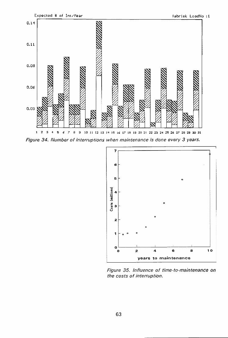
5. Examples 5.1. Influence of the repair-time distribution ... 5.2. Influence of voltage solidity 5.3. Influence of maintenance
Industrial power systems transport electrical energy from the public grid and/or local generators to industrial plants. These plants are often characterized by high costs of interruption, making it necessary to include reliability considerations in the design of these power systems. The reliability considerations become complicated as industrial plants often possess equipment very sensitive to short-duration voltage dips [e.g. 1 ,2,3]. Existing methods for the reliability analysis of electric power systems only include the stationary behaviour after a disturbance (system adequacy [41 or structural reliability ("Strukturzuverlassigkeit") [5]) but not the behaviour during the disturbance (system security [41 or functional reliability (Funktionsszuverlassigkeit") [5]}. These methods describe a component failure as the removal of that component from the power system.
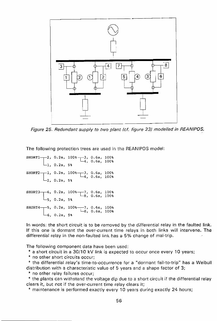
We developed a computer program for reliability analysis of industrial power systems that includes the non-stationary behaviour. In this program called REANIPOS a Monte Carlo method is combined with an electrical network model. The Monte Carlo simulation generates (stochastic) failure and repair events. These events remove and insert branches in the electrical network that represents the electrical behaviour of the primary components of the power system. The electrical network is used to calculate the voltages at the user's positions during an event. The voltage shape during a power system disturbance (i.e. due to an event or a cascade of events generated by the Monte Carlo simulation) is used to determine if a user experiences an interruption.
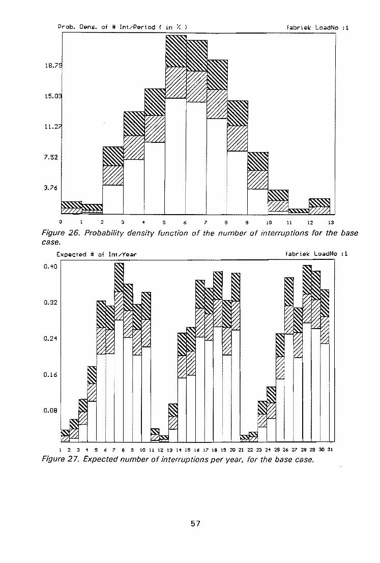
To include the influence of short-duration voltage dips we had to consider in our method short-circuits followed by an intervention of the protection in stead of just the removal of a component. The power system protection is thus explicitly included in the model. Much of what is used to be called "common-mode failures" are actually failures of the protection.
By using a Monte Carlo method the period under consideration {e.g. 30 years) is simulated by generating stochastic fail and restore events. This "simulation of one period" is repeated until enough stochastic data is obtained to estimate the reliability parameters of the electricity supply.
1.1. The interruption criterion.
An interruption criterion is needed to decide whether an event in the power system will lead to an interruption of the supply to a user. Often a logical expression is used for this, relating the state of the components to the state of the system. In this way the transition from one state to the other is not taken into account (i.e. only the adequacy is included, not the security). As e.g. stated in the IEEE Gold Book [8] one needs, for any power system reliability study, a "service interruption definition". The interruption definition specifies the reduced voltage level together with the minimum duration of such a reduced voltage period that results in substantial degradation or complete loss of function of the load or process being served [8].
To include the disturbance behaviour we introduce the maximum permissable voltage dip as an interruption criterion. After each event the voltage at the plant busses is calculated by using the electrical network. If the voltage comes below the maximum permissable
1
voltage dip, the user experiences an interruption of the electricity supply. The concept of the "maximum-permissable voltage dip" is based on the work described in [9]. With reference to the author of [9] we often refer to the maximum-permissable dip as "Spijkers Curve".
Each industrial plant can withstand a voltage zero only for a limited time. A voltage dip of less than 1 p.u. can be withstood for a longer period. If the dip becomes less than a certain value, the plant will never experience an interruption. Observation of existing plants confirms this idea of a "maximum permissable voltage dip" [1 ,2,3]. The duration of permissable dips strongly depends on the type of equipment used in the plant. Some plants can withstand a voltage zero for minutes, others only for a few milliseconds [10]. Within REANIPOS each load is modelled as a constant impedance in the electrical network between ground and the load node (representing the plant bus). As an interruption criterion for each load, the "maximum permissable voltage dip" at the load node is used. If the voltage gets below the maximum-permissable voltage dip, the load experiences an interruption.
1.2. The power system model.
The power system model used for REANIPOS consists of a number of stochastic components and an electrical network. The electrical network is used to calculate the voltages at the load nodes. Branches and nodes of the electrical network are removed and inserted by events in the stochastic components. These stochastic events are generated by the Monte Carlo simulation.
The following types of stochastic components are available in REANIPOS: connections; busses; loads; power supplies; protection trees; relays; automatic transfer systems; maintenance blocks; dependent connections; common-mode failures.
Each Connection has one corresponding branch in the electrical network. A connection consists of a number of sections each possessing a number of possible failures and a number of possible short circuits. It can be incorporated in a number of maintenance blocks. Each failure/short circuit has its own distribution for time-to-occurrence and timeto-repair. If a failure or short circuit occurs the branch is removed from the electrical network (in the latter case due to a relay action) and the faulted section will be repaired. After the repair the branch is inserted in the electrical network again.
Each Bus has one corresponding node in the electrical network. Like a section, a bus possesses a number of possible failures and a number of possible short-circuits, and it can be incorporated in a number of maintenance blocks. If a failure or short circuit occurs the node is removed from the electrical network (i.e. all branches connected to
2
that node are removed), all failures and short circuits are repaired, and the node is inserted again.
Loads represent the different plants or parts of a plant fed from the power system under study. Each load has one corresponding branch between ground and the "load node" in the electrical network. This branch is removed if the supply to this load fails according to the interruption criterion. The voltage on the load node is used for this interruption criterion.
A protection tree links a short circuit with the relays that have to intervene or that might intervene during that short circuit.
Power supplies are voltage sources in the electrical network. These voltage sources cannot be removed.
Relays react on short-circuits and remove branches and/or nodes from the electrical network. They can fail by not tripping when necessary or by tripping when not allowed.
Automatic transfer systems are able to place a branch between two nodes in the electrical network a specific time after another branch is removed from the network. An automatic transfer system can fail by not closing when needed.
Maintenance blocks remove branches from the electrical network in order to make sections, busses, relay systems and automatic transfer systems as good as new.
Dependent connections can be used to define an n out of k system for the connections.
Common-mode failures can be used to link fault events to each other.
1.3. Contents of this report.
This report will describe the computer program REANIPOS in detail. It is intended to be a description of the ideas incorporated in the program as well as a guide for those using the program.
Chapter 2 will describe the mathematics behind the program. It contains some background of the Monte Carlo simulation method; some thoughts about the different distributions used; and a few details about the voltage calculation.
Chapter 3 gives details about the power system model used. All components and events in the program are discussed here.
Chapter 4 explains how the REANIPOS program can be used. It gives the protocol for the ASCII data files that REANIPOS uses as input and output (for those with strong nerves). Chapter 4 also spends a section on the REANEDIT program (to generate and update the input file) and on the REANVIEW program (to analyze the output file).·
Chapter 5 describes a few simple studies performed by using REANIPOS.
3
2. Theoretical background.
2.1 Principle of the Monte Carlo simulation.
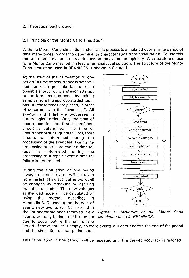
Within a Monte-Carlo simulation a stochastic process is simulated over a finite period of time many times in order to determine its characteristics from observation. To use this method there are almost no restrictions on the system complexity. We therefore chose for a Monte Carlo method in stead of an analytical solution. The structure of the Monte Carlo simulation used in REANIPOS is shown in Figure 1.
At the start of the "simulation of one period" a time of occurrence is determined for each possible failure, each possible short circuit, and each attempt to perform maintenance by taking samples from the appropriate distributions. All these times are placed, in order of occurrence, in the "event list". All events in this list are processed in chronological order. Only the time of occurrence for the first failure/short circuit is determined. The time of occurrence of subsequent failures/short circuits is determined during the processing of the event list. During the processing of a failure event a time-torepair is determined, during the processing of a repair event a time-tofailure is determined. ·
During the simulation of one period always the next event will be taken from the list. The electrical network will be changed by removing or inserting branches or nodes. The new voltages at the load node will be calculated by using the method described in Appendix B. Depending on the type of event, new events will be inserted in the list and/or old ones removed. New Figure 1. Structure of the Monte Carlo events will only be inserted if they are simulation used in REANIPOS. due to occur before the end of the period. If the event list is empty, no more events will occur before the end of the period and the simulation of that period ends.
This "simulation of one period" will be repeated until the desired accuracy is reached.
4
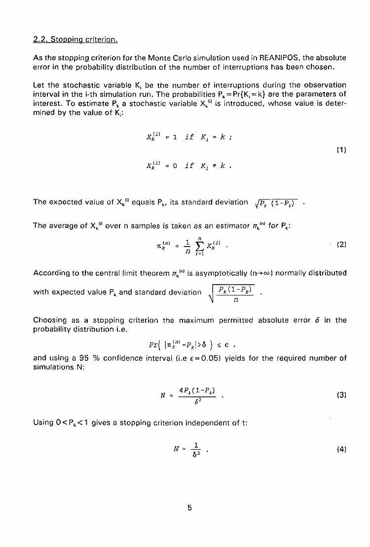
2.2. Stopping criterion.
As the stopping criterion for the Monte Carlo simulation used in REANIPOS, the absolute error in the probability distribution of the number of interruptions has been choseo.
Let the stochastic variable K; be the number of interruptions during the observation interval in the i-th simulation run. The probabilities Pk = Pr{K; = k} are the parameters of interest. To estimate Pk a stochastic variable Xk1;1 is introduced, whose value is determined by the value of K;:
1 if K· = k ; 1.
( 1 )
X (i) 0 'f k k = 1. Ki * ·
The expected value of Xk1;1 equals Pk, its standard deviation JPk ( 1-Pk)
The average of xkm over n samples is taken as an estimator nk1n1 for Pk:
n
1t (n) - 1 "x<i) k --LJk. n i=l
(2)
According to the central limit theorem nklnl is asymptotically (n~oo) normally distributed
with expected value Pk and standard deviation
Choosing as a stopping criterion the maximum permitted absolute error t5 in the probability distribution i.e.
Pr{ 11tknl -Pkl>o } s e ,
and using a 95 o/o confidence interval (i.e f = 0.05) yields for the required number of simulations N:
N (3)
Using 0 < P k < 1 gives a stopping criterion independent of t:
N (4)
5
2.3. Random numbers and distributions.
2.3.1. Failure of components.
The failure behaviour of a component can be described by means of any of the three following functions of time:
probability distribution function F(t) probability density function f(t) failure rate .A(t)
The probability distribution function (of the time to failure) is defined as the probability that the component fails before or on time t, assuming that its lifetime started at time 0:
F( t} Pr{Ts. t} . (5)
The probability density function (of the time to failure) is a measure for the probability that a component whose life started ar time zero will fail around timet for the first time. More precisely:
lim 1 A f{t) = l\tlO l\tPr{t<Ts.t+u.t} (6)
The failure rate .A(t) is a measure for the probability that a component that has not failed before time t will fail soon after. More precisely:
l(t} = l~to ftPr{Ts.t+AtiT>t} (7)
Each of these functions can be expressed into the two others by means of the following equations:
l { t) = - ddt ln{l-F( t)}
6
f( t)
f f (,;) d,; t
{8)
(9)
(1 0)
2.3.2. The random number generator.
From the standard uniform distribution (the uniform distribution on the interval [0, 1] ) samples from all other probability distributions needed can be drawn. These distributions are used in the Monte Carlo simulation to generate times of failure and times of repair.
Let U be a stochastic variable with a standard normal distribution. A sample from a stochastic variable X with distribtion function F(x) can be drawn by using:
( 11 )
A sample from the standard uniform distribution is taken by using a "random number generator". By using a mathematical expression a pseudo-random sequence of numbers is generated. Many expressions have been proposed in the past. We have chosen the one proposed by Fishman and Moore [6]:
where a= 950706376 and N = 231 -1.
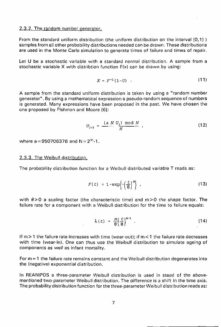
2.3.3. The Weibull distribution.
(aN UJ mod N
N
The probability distribution function for a Weibull distributed variable T reads as:
(12)
(13)
with 8>0 a scaling factor (the characteristic time) and m>O the shape factor. The failure rate for a component with a Weibull distribution for the time to failure equals:
1.. ( t} (14)
If m > 1 the failure rate increases with time (wear-out); if m < 1 the failure rate decreases with time (wear-in). One can thus use the Weibull distribution to simulate ageing of components as well as infant mortality.
For m = 1 the failure rate remains constant and the Weibull distribution degenerates into the (negative) exponential distribution.
In REANJPOS a three-parameter Weibull distribution is used in stead of the abovementioned two-parameter Weibull distribution. The difference is a shift in the time axis. The probability distribution function for the three-parameter Weibull distribution reads as:
7
F( t) = 1-exp { - ( ~=~ r} I t-zy. I { 15)
where y is the minimum value of the time to failure, and 9?:. y.
Using (11) and (15) we conclude that for a uniform distributed stochastic variable U
W Y + (8 y} m~ - ln ( U) {16)
has a Weibull distribution with minimum value y, characteristic value f/, and shape factor m.
2.3.4. The bathtub distribution.
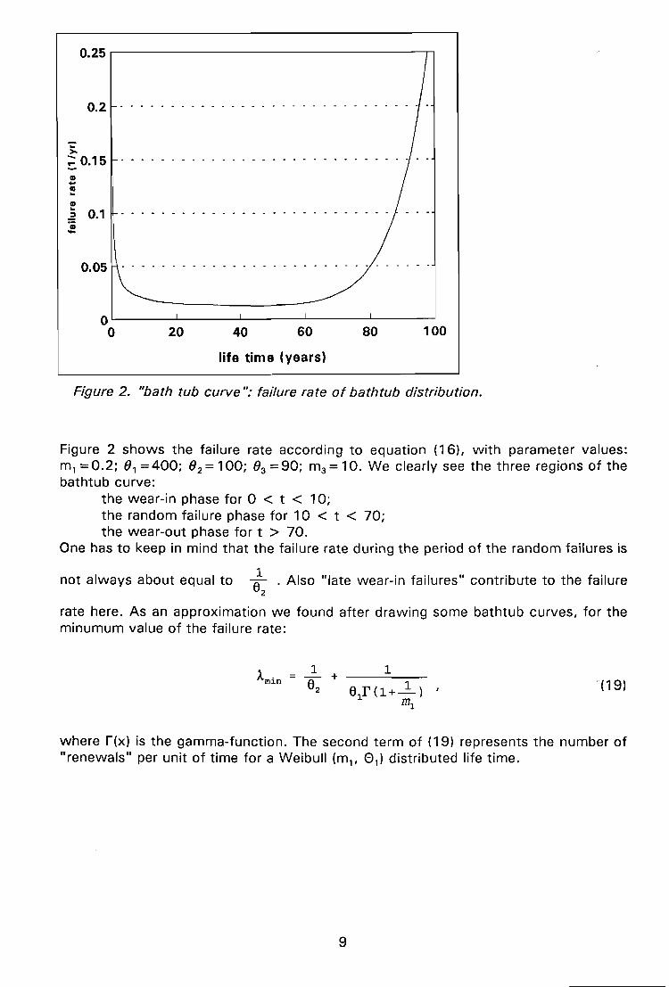
To describe the failure behaviour of components often the "bath tube" curve is used. The bath tub curve gives the typical behaviour of the failure rate of a component. During the infant mortality (wear-in) period the failure rate is high but decreases fast. During the component's normal life the failure rate is constant and determined by external processes. During the wear-out period the failure rate increases again. An example of a bath tub curve is shown in figure 2 below.
In REANIPOS the failure rate of the bath tub distribution is considered to be the sum of the failure rates of three weibull distributions, with shape factor smaller than one, equal to one and larger than one.
( 17)
with 0 < m1 < 1 and m3 > 1. The corresponding probability distribution function reads as:
F( t) { ( t )ml t ( t )m3 }
1 - exp - (\ - e; - a; · ( 18)
A sample from the bathtub distribution is determined as the smallest value of three samples from the three underlying Weibull distributions.
In REANIPOS the user can introduce a time-shift for the bathtub like for the Weibull distribution. The three underlying Weibull distribution of the bathtub should have the same time shift. The consequence of this time shift is that no events can occur before a predetermined instant.
This way of modelling the bath tub has some disadvantages for the user. It is used because its implementation turned out to be relatively simple in REANIPOS. The user therefore has to keep in mind that using the bathtub for component failures might leads to unexpected results (at least that's our experience). We will present one example of a bathtub curve here to indicate where some of the danger lies.
Figure 2. "bath tub curve": failure rate of bathtub distribution.
Figure 2 shows the failure rate according to equation (16), with parameter values: m, = 0.2; O, = 400; 02 = 1 00; 03 = 90; m3 = 10. We clearly see the three regions of the bathtub curve:
the wear-in phase for 0 < t < 1 0; the random failure phase for 10 < t < 70; the wear-out phase fort > 70.
One has to keep in mind that the failure rate during the period of the random failures is
not always about equal to ~ . Also "late wear-in failures" contribute to the failure 2
rate here. As an approximation we found after drawing some bathtub curves, for the minumum value of the failure rate:
= 1 + ~
1 '(19)
where r(x) is the gamma-function. The second term of (19) represents the number of "renewals" per unit of time for a Weibull (m 1 , 8 1 ) distributed life time.
9
The table below gives the value of r ( 1 +..!.) for different values of m ::s; 1. m
Figure 3: probability distribution function for the bathtub of Figure 2.
Figure 3 shows the probability distribution function corresponding to the bathtub of figure 2. We can see here that about 50% of the failures occur during the wear-in phase, about 20% during the wear-out phase and the remaining 30% during the random failures period. If the characteristic time of the first term of the distribution (0 1) is decreased (or its shape factor increased) the percentage of failures during the wear-in period will increase, leaving little room for random failures and even less for wear-out failures. In that case it is of no use including the latter in the model.
10
N.B. This reasoning only holds when the component is repaired "as good as new". When the component is repaired "as bad as old" it will always reach the wear-out phase (cf. section 2.2.8).
Figure 4. Probability density function for bathtub of Figure 2.
Finally figure 4 shows the probability density function f(t) for the bathtub of figure 2. One notices a clustering of times-to-failure around time-zero and around time equals 90.
2.3.5. The normal distribution.
The normal distribution is defined through its probability distribution:
f(t) = 1 exp{-(..!=H.)2},
o../2rt a (20)
where J1 is the expected value and a the standard deviation of the normal distribution.
Since the probability distribution function F of the normal distribution can only be numerically inverted we prever to use the Box-Muller method [12] (in stead of (11) ) in sampling from the normal distribution:
(21)
where X is a sample from the normal distribution with expected value J1 and standard deviation a; U, and U2 are independent samples from the standard uniform distribution.
1 1
In REANIPOS the user can introduce a minimum time-to-occurrence for the normal distribution. The distribution is not shifted in time like has been done for the Weibull distibution, but the left part of the distribution will be cut-off. This has to be done to prevent negative times. The minimum value therefore has to be non-negative.
If a sample X from the normal distribution turns out to be below the minimum value, it is rejected and a new sample is taken.
2.3.6. The uniform distribution.
The uniform distribution m[T1, T2]is defined through its probability density:
(22)
where T 1 and T 2 are lower limit and upper limit of the time to failure, respectively.
According to (11) A sample X from the uniform distribution is determined by:
(23)
with U a sample from the standard uniform distribution.
2.3.7. A chance.
In some models an event takes place with a certain probability or chance p. Simulation of this situation is modelled by:
U<p U>p
event occurs event does not occur
(24)
where U is a sample from the standard uniform distribution and p is the probability that the event occurs.
2.3.8. Repair "as good as new" or "as bad as old".
When a component fails it will be repaired. In case of "perfect" repair the failure rate of the repaired component will be like a fully new component (often the failed component is indeed replaced by a new one). The component will then be "as good as new". This implies that a new time-to-failure can be determined as a sample from the original life time distribution. In some cases the component immediately after the repair has the same failure rate as the component immediately before the failure. The component is then "as bas ad old". In that case the REANIPOS simulator takes a sample from the original life time distribution, subtracts from this the time elapsed since the start of the simulation, and rejects the result if the new time to failure is below zero. In that case the drawing is repeated till a positive time results.
12
Thus after repair "as-good-as-new" a time-to-failure is determined from the life-time distribution, after repair "as-bad-as-old" a time-of-failure is determined.
WARNING: the user should keep in mind that distributions with a high failure rate in combination with repair "as bad as old" lead to a high number of failures. The uniform distribution even leads to an infinite number of failures in a finite time. When using repair "as-bas-as-old" the user should for the time-to-failuire never use a uniform distribution with an upper limit less than the duration of the period under study. This will lead to an infinite number of failures in one period. The user is further adviced not to use a Weibull distribution with a high shape factor (m > 2) and a characteristic value less than the duration of the period under consideration. This might lead to a very high number of failures in one period.
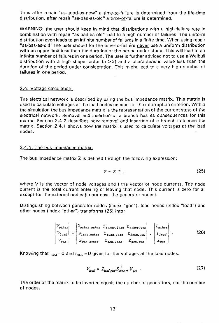
2.4. Vqltage calculation.
The electrical network is described by using the bus impedance matrix. This matrix is used to calculate voltages at the load nodes needed for the interruption criterion. Within the simulation the bus impedance matrix is the representation of the current state of the electrical network. Removal and insertion of a branch has its consequences for this matrix. Section 2.4.2 describes how removal and insertion of a branch influence the matrix. Section 2.4. 1 shows how the matrix is used to calculate voltages at the load nodes.
2.4.1. The bus impedance matrix.
The bus impedance matrix Z is defined through the following expression:
V=ZI, (25)
where V is the vector of node voltages and I the vector of node currents. The node current is the total current entering or leaving that node. This current is zero for all except for the external nodes (in our case the generator nodes).
Distinguishing between generator nodes (index "gen"), load nodes (index "load"} and other nodes (index "other") transforms (25) into:
vother zother. other zother .load Zother.gen I other
vload = zload.other zload.load zload.gen I load _. (26)
vgen Zgen.other Zgen.load Zgen.gen Igen
Knowing that l,oad = 0 and I other= 0 gives for the voltages at the load nodes:
(27)
The order of the matrix to be inverted equals the number of generators, not the number of nodes.
13
In REANIPOS the user creates the "other nodes" whereas the simulator creates the load nodes and the generator nodes (ct. 3.4 and 3.5).
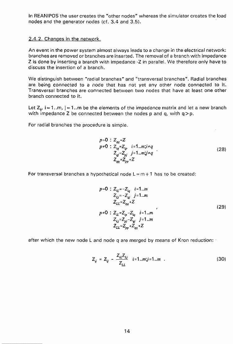
2.4.2. Changes in the network.
An event in the power system almost always leads to a change in the electrical network: branches are removed or branches are inserted. The removal of a branch with impedance Z is done by inserting a branch with impedance -Z in parallel. We therefore only have to discuss the insertion of a branch.
We distinguish between "radial branches" and "transversal branches". Radial branches are being connected to a node that has not yet any other node connected to it. Transversal branches are connected between two nodes that have at least one other branch connected to it.
Let Zii• i = 1 .. m, j = 1 .. m be the elements of the impedance matrix and let a new branch with impedance Z be connected between the nodes p and q, with q > p.
For radial branches the procedure is simple.
p=O : Zqq=Z P*O : Ziq=Zip i=1 .. m;i*q
Zqj=ZPi j=1 .. m;j*q Zqq=ZPP+Z
For transversal branches a hypothetical node L = m + 1 has to be created:
p=O : ZiL =-Ziq i=1 .. m ZLj=-Zqj j=1 .. m Zu=Z +Z qq
P*O: ZiL=Zip-Ziq i=1 .. m zL1=ZprZqj j=1 .. m ZLL =Zpp +Zqq +Z
after which the new node Land node q are merged by means of Kron reduction:
14
(28)
(29)
(30)
3. The power system model.
This chapter will describe how the events generated by the Monte Carlo simulation are treated. All components and events will be discussed here. The chapter will end with the relations between the different events.
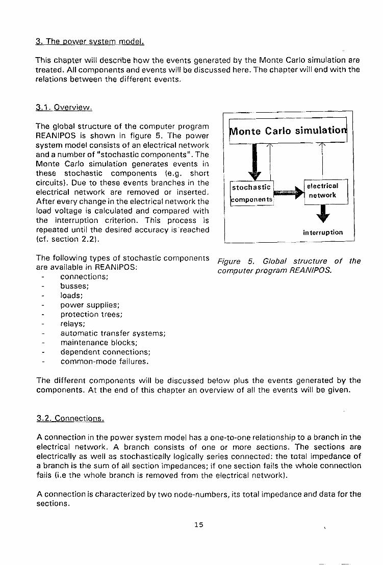
3.1. Overview.
The global structure of the computer program REANIPOS is shown in figure 5. The power system model consists of an electrical network and a number of "stochastic components". The Monte Carlo simulation generates events in these stochastic components (e.g. short circuits}. Due to these events branches in the electrical network are removed or inserted. After every change in the electrical network the load voltage is calculated and compared with the interruption criterion. This process is repeated until the desired accuracy is ·reached (cf. section 2.2).
The following types of stochastic components Figure 5. Global structure of the are available in REANIPOS: computer program REANIPOS.
connections; busses; loads; power supplies; protection trees; relays; automatic transfer systems; maintenance blocks; dependent connections; common-mode failures.
The different components will be discussed below plus the events generated by the components. At the end of this chapter an overview of all the events will be given.
3.2. Connections.
A connection in the power system model has a one-to-one relationship to a branch in the electrical network. A branch consists of one or more sections. The sections are electrically as well as stochastically logically series connected: the total impedance of a branch is the sum of all section impedances; if one section fails the whole connection fails (i.e the whole branch is removed from the electrical network).
A connection is characterized by two node-numbers, its total impedance and data for the sections.
15
Four types of sections can be present in a connection: normal sections (cf. 3.2.1 ); load sections (cf. 3.4); generator sections (cf. 3.5); ATS sections (cf. 3.8).
3.2.1. Normal sections.
A normal section can posses a number of possible failures or short circuits, and can be incorporated in a number of maintenance blocks. Each failure and each short circuit has its own distribution for time to failure and for time to repair. If a failure or short circuit occurs the branch is removed from the electrical network and the whole section is repaired; i.e. new times to failure are determined for all possible failures and short circuits.
REANIPOS distinguishes between a "failure" leading to the immediate removal of the branch involved and a "short circuit" leading to the insertion of a low-impedance branch to ground followed by the removal of the faulted branch plus eventually other branches by protective relays. More details about failures and about short circuits can be found in the following sections.
Maintenance can be performed on a section. A section can be part of several maintenance blocks. After the maintenance has been performed a new time to failure is determined. For the determination of a new time-to-failure (after repair or maintenance) one can choose between repair being "as good as new" or repair being "as bad as pld". More details about maintenance are given in section 3.9.
Warning: unexpected things can happen if in a section two failures take place, one of which is repaired as-bad-as-old and the other as-good-as-new. Suppose failure 1 is repaired as-good-as-new and failure 2 as-bad-as-old. If failure 1 takes place, a repair time is determined from the corresponding distribution. The whole section is in this case repaired "as-good-as-new", i.e both for failure 1 and for failure 2 times-tQ-failure will be determined from the original distribution. If failure 2 takes place the whole section will be repaired as-bad-as-old; i.e for failure 2 a new time-of-failure will be determined and for failure 1 no new time has to be determined.
3.2.2. Failures.
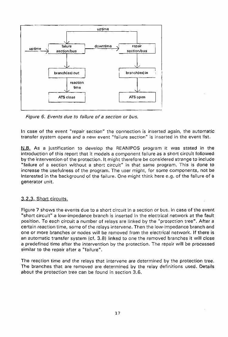
Figure 6 shows the events due to the failure of a section or bus. During the initiation of the event list a time-to-occurrence is determined for each possible "failure". The events in the event list are then processed one by one (ct. 2.1).
In case of the event "failure of a section" the branch to which the section belon.gs is removed from the electrical network. It there is an automatic transfer system linked to this branch (ct. 3.8) it will close after a predetermined reaction time (unless the automatic transfer system fails). Next a repair time is determined and the event "repair section" is inserted in the event list.
16
uptime
downtime repair section/bus
Figure 6. Events due to failure of a section or bus.
In case of the event "repair section" the connection is inserted again, the automatic transfer system opens and a new event "failure section" is inserted in the event list.
N.B. As a justification to develop the REANIPOS program it was stated in the introduction of this report that it models a component failure as a short circuit followed by the intervention of the protection. It might therefore be considered strange to include "failure of a section without a short circuit" in that same program. This is done to increase the usefulness of the program. The user might, for some components, not be interested in the background of the failure. One might think here e.g. of the failure of a generator unit.
3.2.3. Short circuits.
Figure 7 shows the events due to a short circuit in a section or bus. In case of the event "short circuit" a low-impedance branch is inserted in the electrical network at the fault position. To each circuit a number of relays are linked by the "protection tree". After a certain reaction time, some of the relays intervene. Then the low-impedance branch and one or more branches or nodes will be removed from the electrical network. If there is an automatic transfer system (cf. 3.8) linked to one the removed branches it will close a predefined time after the intervention by the protection. The repair will be processed similar to the repair after a "failure".
The reaction time and the relays that intervene are determined by the protection tree. The branches that are removed are determined by the relay definitions used. Details about the protection tree can be found in section 3.6.
17
uptime
'\ I/ reaction downtime uptime '\ short-circuit time '\ intervention __'\ repair L
/ section/bus / by protection 7 section/bus I
t ~ s/ '\I/ short-circuit
I short-circuit
branch in branch out branch(es) out branch{es} in
reaction time
'\ I/ '\ I/
ATS close ATSopen
Figure 7. Events due to a short circuit in a section or bus.
load
no do
Figure BA. Branch in REANIPOS's electrical network before a short circuit.
i
Figures SA through SC show what happens meanwhile in the electrical network. A healthy connection consists of a number of section impedances in series (figure SA). When a short circuit occurs in one of the sections that section will be split in two and the newly created node is connected to ground by a low-impedance branch (figure SB}. When the protection intervenes the whole branch is removed from the electrical network (figure SC). After a certain repair time this branch is inserted in the network again {back to figure SA).
Contrary to what is suggested by the figure, REANIPOS does not create new nodes in the electrical network nor remove any existing nodes. In the top situation the three
18
Figure 8B. Branch in REANIPOS's electrical network during a short circuit.
Figure BC. Branch in REANIPOS's electrical network after a short circuit.
sections are combined to one impedance; in the centre situation each section and a half is combined to one impedance. The "removal of a node" (e.g. after intervention of a relay) does not actually imply the removal of that node form the electrical network, but the removal of all branches that are connected to the node. As each node is connected to ground through a high-impedance branch, the node voltage is always defined.
3.3. Busses.
Each bus has one corresponding node in the electrical network. Like a section a bus can possess a number of possible short circuits and failures. If a failure or short circuit occurs the node is "removed" (i.e. all branches leading to that node are removed from the electrical network), all failures and short circuits are repaired and the node is inserted again.
3.4. Loads.
Figure 9 shows the network representation of a connection with a load section. The corresponding two branches in series connection are present between ground and one of the "other nodes" as introduced in 2.4.1. The connection consists of a load section (between ground and the "load node") plus one or more normal sections. The voltage at the load node is used for the interruption criterion (ct. 3.4.1 ). This connection is
19
represented by two branches in the electrical network: one branch between ground and the load node; one branch between the load node and the other node. The branch between the load node and the other node is removed if the load experiences an interruption.
A load can experience an interruption because the voltage at the load node does not meet the interruption criterion or because some other load fails on which the current load is dependent. The user can set a time between the interruption of the load and the interruption of the original load.
NODE
,--1
I
I 1 I I I I I I I I I
I I I I
normal sections
I I I
I I I I I I I
load node I
load sections
_____ .J
The interruption is considered over if the branch to the load
Figure 9. Connection with a load section. node, plus those branches for all the dependent loads, can be inserted in the electrical network without violating the interruption criterion of any of these loads.
Warning: If more than one load experiences an interruption, first the branch to the load node with the highest number is inserted in the electrical network (if possible), the other loads follow. The duration of interruption might therefore be longer for loads with a lower load number than for loads with a higher load number, in an otherwise symmetrical system.
3.4.1. The interruption criterion.
Each industrial plant can withstand a voltage zero only for a limited time. A voltage dip of less than 1 p.u. can be withstood longer. If the dip becomes less than a certain value, the plant will never experience an interruption. Observations of existing plants confirm the idea of a "maximum permissable voltage dip". The duration of permissable dips strongly depends on the type of equipment used in the plant. Some plants can withstand a voltage zero for minutes, others only for a few milliseconds.
Within REANIPOS each load is modelled as a constant impedance in the electrical network between ground and the load node (representing the plant bus). As an interruption criterion for each load, the "maximum permissable voltage dip" at the load node is used. If the voltage gets below the maximum permissable voltage dip, the load experiences an interruption. Figure 10 gives an example of the use of the interruption criterion. The solid line· gives the maximum-permissable voltage dip; the dotted ·lines
20
voltage
1p.u.-
. . . . ~ I· . . . . '3
. . 0 11me
Figure 10. Use of interruption criterion of REANIPOS.
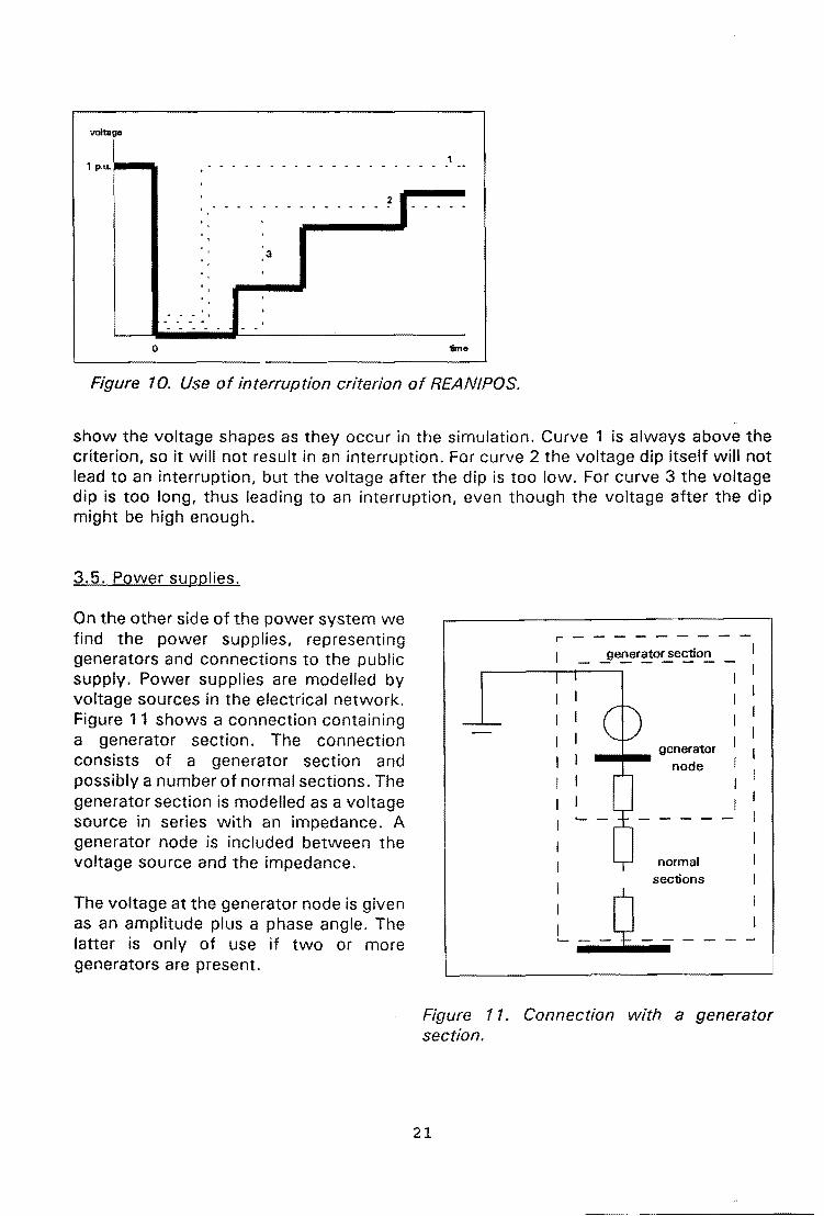
show the voltage shapes as they occur in the simulation. Curve 1 is always above the criterion, so it will not result in an interruption. For curve 2 the voltage dip itself will not lead to an interruption, but the voltage after the dip is too low. For curve 3 the voltage dip is too long, thus leading to an interruption, even though the voltage after the dip might be high enough.
3.5. Power supplies.
On the other side of the power system we find the power supplies, representing generators and connections to the public supply. Power supplies are modelled by voltage sources in the electrical network. Figure 11 shows a connection containing a generator section. The connection consists of a generator section and possibly a number of normal sections. The generator section is modelled as a voltage source in series with an impedance. A generator node is included between the voltage source and the impedance.
The voltage at the generator node is given as an amplitude plus a phase angle. The latter is only of use if two or more generators are present.
r---------generator section I
r------.-r---.- - - - - I
I
I normal
~ Q ·~~·-- ~ Figure 11. Connection with a generator section.
21
3.6. Protection trees.
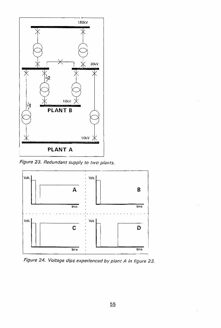
In case of a short circuit one or more primary relays are supposed to isolate the short circuit from the healthy part of the power system. If such a relay fails one or more backup relays take over the protection. Each backup relay also has one or more backup relays itself. This results in a "protection tree" for each short circuit. Within REANIPOS this protection tree is used to describe the behaviour of the protection. Consider as an example the power system of figure 12, where the circles denote differential relays and the squares over-current time relays. Figure 13 gives the protection tree for a fault at position A in figure 12. The ATS is at first considered to be in the closed position. (The situation for open A TS is discussed in 3.8.1.) Each position in the protection tree (as shown in figure 13) has a probability of operation and a time to operation. Relay 1 serves as a primary relay for short circuit A. If it is not
1 2
ATS
PLANT A
Figure 12. Redundant supply to two plants, with differential relays (circles) and over-current time relays (squares).
dormant (cf. 3. 7) it will disconnect the short circuit with a probability of 100% 0.2 seconds after fault initiation. Relays 2, 3, and 4 (differential relays in healthy connections) have a low probability of operation, in this example 5% has been arbitrarily chosen. The operation of one of the latter relays clearly is a mal-trip.
If relay 1 fails (in this case: if it is dormant) its backup relays will take over the protection: relay 5 and relay 6 {both over-current time relays) will intervene 0.8 seconds after fault-initiation with a probability of 100% and 70%, respectively. The lower probability for relay 6 is to represent short circuits close to the medium-voltage bus that will not be detected by the over-current time relay in the parallel connection. If one of the relays 5 and 6 fails, over-current time relays 7 and 8 will intervene, 1.2 seconds after fault initiation.
The reaction time of the protection is taken equal to the reaction time of the last relay that intervenes, according to the protection tree. At that moment all relays are considered to intervene, i.e. all relevant branches are removed from the electrical
22
network. The faulted branch is always removed from the electrical network if at least one relay intervenes, even if this relay is not supposed to remove that branch.
Warning: the user has to keep in mind that if no relay at all reacts, the short circuit will never be cleared (i.e. it will stay there maybe for tens of years). The user should therefore always include one or more relays that never fail in the protection tree to ensure the operation of at least one relay.
One possibility is to create a relay Figure 13. Protection tree for fault A in figure 12 that isolates all generators from (when the A TS is in the closed position). the power system, and to include this at the end of all relevant branches of the protection tree. Another possibility is to make the first level of backup relays 100% reliable (i.e to neglect failure of a backup relay). The latter solution will simplify the protection trees considerably, especially for large systems, without, in most cases, significantly influencing the results.
3. 7. Relays.
A relay in REANIPOS removes, upon intervention, one or more branches or nodes from the electrical network. This intervention normally takes place when a short circuit occurs for which the relay is supposed to intervene (it is linked to that short circuit by the protection tree as described in 3.6}.
The relay can fail by showing an incorrect trip or by getting into a "dormant fail-to-trip" state. An incorrect trip leads to the immediate removal of a branch from the electrical network. If the relay is dormant (i.e. in the "dormant fail-to-trip" state} it will not intervene when supposed to. It's backup relay or relays (if present) will then take over the protection.
The relay can further fail by intervening during a short circuit for which it is supposed to refrain from action. These failures are included in the protection tree (cf. 3.6).
3.8. Automatic transfer systems.
An automatic transfer system (ATS) is a normally open switch between two busses that closes if the supply to one of the busses fails. The model ATS in REANIPOS is supposed to close if one branch from a group of branches is removed from the electrical network. This removal of a branch is either due to a failure of a section, due to intervention of a relay or due to maintenance. Between the removal of the branch and the closing of the
23
switch, a certain reaction time has been assumed. For an automatic transfer system the reaction time will be a few seconds, for a manual switch the reaction time is up to a few hours. For closing due to maintenance a reaction time equal to zero is assumed.
low-node high-node
~~b~ I ____ J I I normal normal
ATSsection 1 sections section
Figure 14. Connection with an A TS section.
Figure 14 shows a connection containing an ATS section. Such a connection consists of: possibly a number of normal sections; an ATS section and one or more normal sections.
An automatic transfer system can fail by getting into a dormant fail-to-trip state. It will then not close when supposed to. The ATS can get out of this dormant state by maintenance and by repair. During maintenance and during the repair the automatic transfer system does not operate when supposed to.
If the ATS is supposed to intervene but in a dormant state, a repair time is determined. When the repair is finished, and the closure of the ATS remains necessary, it will still close.
3.8.1. ATS option relays.
When an ATS closes, the system is changed and often the protection trees for some of the possible short circuits as well: i.e. other or more relays are supposed to intervene. To include this in the reliability analysis, REANIPOS possesses an "ATS option" for each of the relays in the protection tree. If a certain ATS is in the closed position, some relays in the protection tree are replaced by their ATS option.
The "ATS option relays" have a probability of operation and a time-to-operation, like the normal relays. They also have a "switch back time". A certain time after the ATS option relay intervened, the ATS switch will open and the branches removed by the ATS option relay will be inserted again.
Consider again the power system shown in figure 12. When the ATS is in the open position, the protection tree will be different from the one shown in figure 13: relay 2 will no longer have a chance of mal-trip, nor will relay 6 serve as a back-up. To incorporate this in REANIPOS a dummy relay is introduced (here denoted by the number 99) that never fails and that does not remove any branch when it "intervenes". These dummy relays are present in the protection tree when the ATS is in the open position.
24
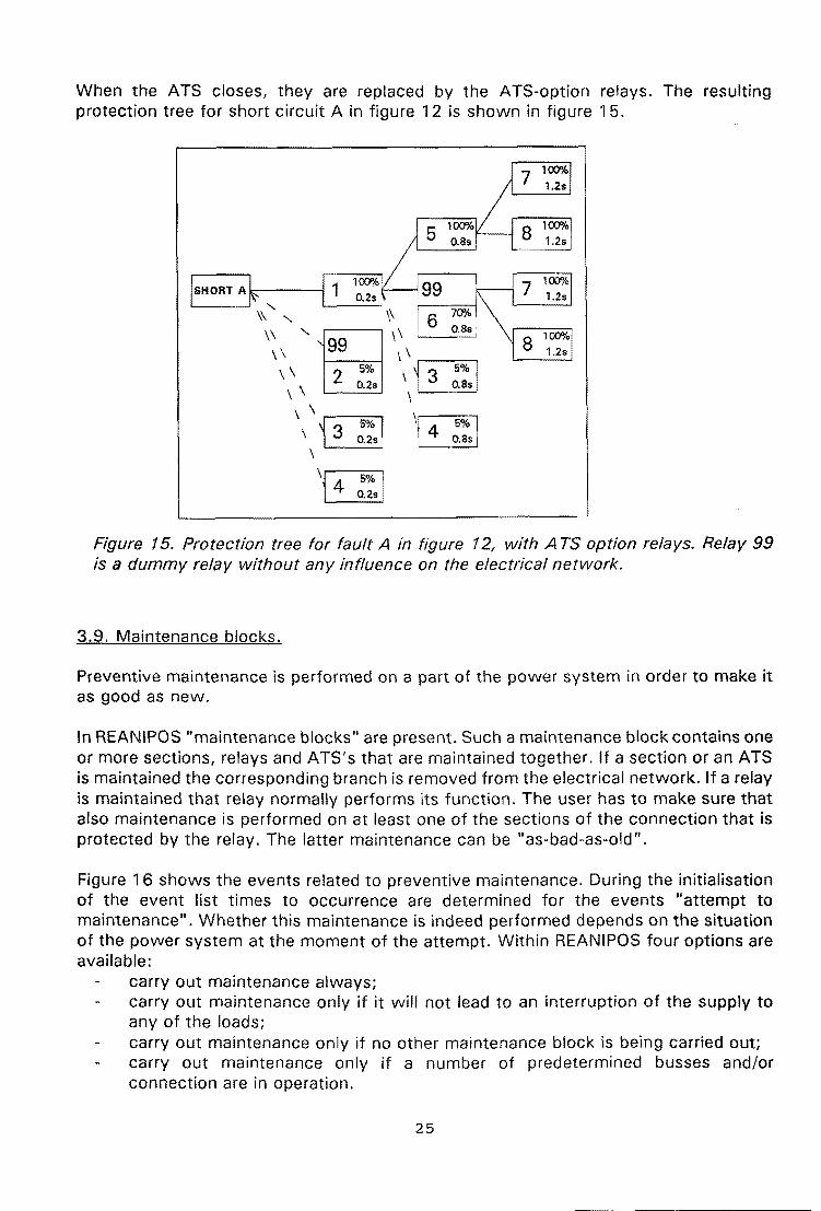
When the ATS closes, they are replaced by the ATS-option relays. The resulting protection tree for short circuit A in figure 12 is shown in figure 15.
\~ ~
'r-;;5%l ~
Figure 15. Protection tree for fault A in figure 12, with A TS option relays. Relay 99 is a dummy relay without any influence on the electrical network.
3.9. Maintenance blocks.
Preventive maintenance is performed on a part of the power system in order to make it as good as new.
In REANIPOS "maintenance blocks" are present. Such a maintenance block contains one or more sections, relays and ATS's that are maintained together. If a section or an ATS is maintained the corresponding branch is removed from the electrical network. If a relay is maintained that relay normally performs its function. The user has to make sure that also maintenance is performed on at least one of the sections of the connection that is protected by the relay. The latter maintenance can be "as-bad-as-old".
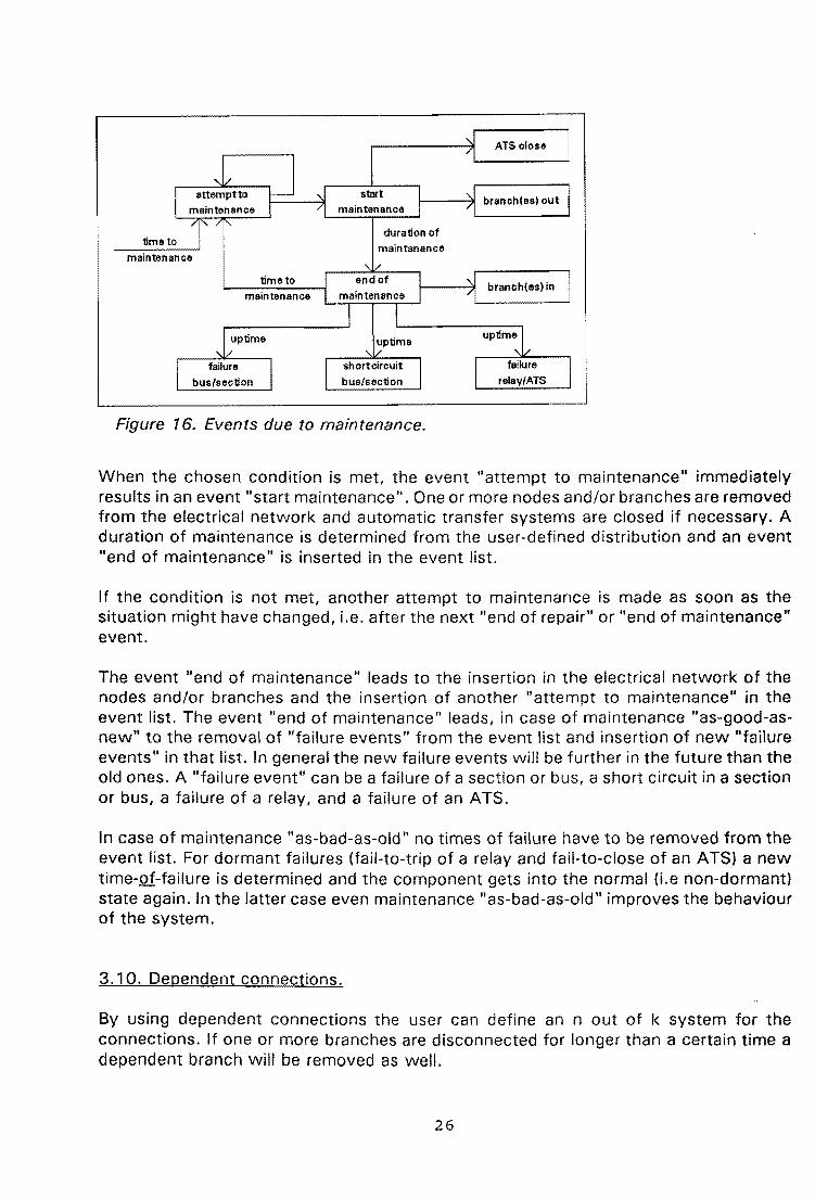
Figure 16 shows the events related to preventive maintenance. During the initialisation of the event list times to occurrence are determined for the events "attempt to maintenance". Whether this maintenance is indeed performed depends on the situation of the power system at the moment of the attempt. Within REANIPOS four options are available:
carry out maintenance always; carry out maintenance only if it will not lead to an interruption of the supply to any of the loads; carry out maintenance only if no other maintenance block is being carried out; carry out maintenance only if a number of predetermined busses and/or connection are in operation.
25
ATS close
time to
maintenance
time to branch( as) in maintenance
Figure 16. Events due to maintenance.
When the chosen condition is met, the event "attempt to maintenance" immediately results in an event "start maintenance". One or more nodes and/or branches are removed from the electrical network and automatic transfer systems are closed if necessary. A duration of maintenance is determined from the user-defined distribution and an event "end of maintenance" is inserted in the event list.
If the condition is not met, another attempt to maintenance is made as soon as the situation might have changed, i.e. after the next "end of repair" or "end of maintenance" event.
The event "end of maintenance" leads to the insertion in the electrical network of the nodes and/or branches and the insertion of another "attempt to maintenance" in the event list. The event "end of maintenance" leads, in case of maintenance "as-good-asnew" to the removal of "failure events" from the event list and insertion of new "failure events" in that list. In general the new failure events will be further in the future than the old ones. A "failure event" can be a failure of a section or bus, a short circuit in a section or bus, a failure of a relay, and a failure of an ATS.
In case of maintenance "as-bad-as-old" no times of failure have to be removed from the event list. For dormant failures (fail-to-trip of a relay and fail-to-close of an ATS) a new time-of-failure is determined and the component gets into the normal (i.e non-dormant) state again. In the latter case even maintenance "as-bad-as-old" improves the behaviour of the system.
3.1 0. Dependent connections.
By using dependent connections the user can define an n out of I< system for the connections. If one or more branches are disconnected for longer than a certain time a dependent branch will be removed as well.
26
if (branch 1 is disconnected for longer than time 1) and (branch 2 is disconnected for longer than time 2) and
and (branch n is disconnected for longer than time n) then branch (n + 1) is removed from the electrical network.
Branch (n + 1) is inserted again if one of the other branches is inserted.
3.11. Common-mode failures.
Common-mode failures can be used to bring a causal link between two fail events; Fail events can be: failure of a section or bus; short circuit in a section or bus; failure of an ATS; failure of a relay.
The common-mode failure ensures that the occurrence of a specified event will lead, with a certain constant probability, to the occurrence of one or more other events after a specified time.
The common-mode failure is repaired as soon as the original failure is repaired.
3.12. Events in the Monte Carlo simulation.
During the simulation two kinds of events take place: initial events and non-initial events. Initial events can take place without any other event having occurred before. Their timesof-occurrence are determined at the start of the simulation of one period. Non-initial events can only take place if another event occurred before. Their times-of-occurrence cannot be determined before that other event takes place. Failure of a component is an initial event, repair of that component a non-initial event.
In REANIPOS the following initial events are present:
a. failure of a section; b. short circuit in a section; c. failure of a bus; d. short circuit in a bus; e. mal-trip of a relay; f. dormant fail-to-trip of a relay; g. dormant fail-to-close of an ATS; h. attempt to maintenance.
These initial events can lead to the following non-initial events: 1. repair of a section; 2. repair of a bus; 3. closure of an ATS; 4. opening of an ATS; 5. repair of an ATS;
27
6. intervention by a relay; 7. repair of a relay; 8. start maintenance; 9. end of maintenance.
Finally there are 4 events related to the voltage calculation and the interruption criterion: A. removal of a branch from the electrical network; B. insertion of a branch in the electrical network; C. start of interruption; D. end of interruption.
e X X f
g
h 0
X X
X
7 X X 8 X X 9 X X X X X X X X X
Every event can lead to one or more other events. The table above shows these relationships. For more details please refer to the component description in this chapter or to the program listing and comments [7].
A cross denotes that the event on the left side always leads to the event on the top (if the relevant component is present in the system). A circle denotes that the left side event might lead to the top side event depending on the momentary state of the system and the electrical network.
Common-mode failures and dependent connections are not included in the table above.
28
4. How to use the REANIPOS simulator.
This chapter is intended as a kind of users manual for the REAI\JIPOS package. At least some of the knowledge contained in the previous chapters is neccessary to understand this chapter. It is therefore not suitable as a stand-alone manual. The structure of the input and output files of REANIPOS will be discussed first. Next, a short description will be given of the REANEDIT input program and of the REANVIEW output program.
4.1. The DOS command line.
The REANIPOS simulator is started through the DOS-command line
REANIPOS INPUT OUTPUT [X] [Y] [ZZZ]
where INPUT is the name of the input file that contains the system data; OUTPUT is the name of the output file where REANIPOS will place the simulation results; [X] is a parameter that determines the amount of data in the output file
[X] = E implies extended output (all events are included} [X] = N implies normal output (interruptions only)
[Y] determines what to do if an error occurs during the execution of the program, for use in a batch file
[Y] = 1 causes the program to stop on an error and wait for a key to be pressed. [Y] = 0 causes a return to the operating system on an error
[ZZZ] (optie) implies extended output to printer on LPT1 from the simulation of period [ZZZ] on.
During normal use of the simulator, the input file is created by the input program REANEDIT, whereas the output file is treated by the output program REANVIEW. Both programs can be used with the knowledge from the previous chapters.
We will however describe both the input file and the output file in detail below. This is to give the user some background that might be needed to use the input program REANEDIT; to make it possible for the user to read the input file for the simulator (this will, in some cases, be faster than using the input program REANEDIT); for special applications not supported by REANEDIT (e.g. dependent connections and commonmode failures); and to make it possible for the user to write his own output program.
4.2 The input file.
The input file of REANIPOS describes the power system to be simulated according to the protocol given in this chapter. The input file is a ("readable") ASCII file. The user of REANIPOS can create the input file by using an editor or word processor or decide to use the interactive input program REANIPOS to generate the file, or any combination of these two options.
29
The following notation has been used in describing the input file:
< .. $> = string variable < .. #> = numerical variable {. I .} = one of the options has to be chosen { ... } = optional [CR] = new line " " subdefinition =
A space between two data means any non-zero number of spaces to seperate the data. No space means absolutely no spaces in the input file (e.g. at the end of the line)
The input file contains the following blocks; a. general data block; b. connection data block; c. bus data block; d. load data block; e. generator data block; f. automatic transfer system data block; g. short circuit data block; h. relay data block; i. event data block; j. maintenance data block; k. distribution data block; I. connection dependency data block; m. common-mode failure data block; n. end.
A few general comments about the input file: a. All lines starting with a star character(*) are comment lines. they can contain up
to 15 characters but no spaces. They are used to seperate the data blocks from each other.
b. In REANIPOS time is always measured in days and/or seconds. The user always has to keep this in mind when creating or reading the file.
All lines starting with a star character ( *) are comment lines. they can contain up to 15 characters but no spaces.
30
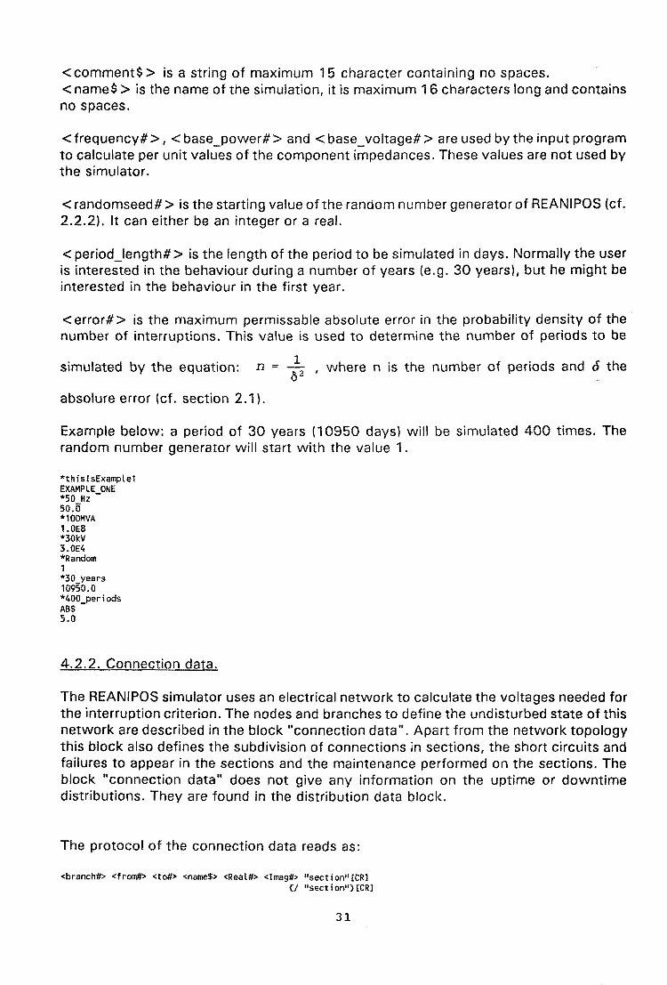
<comment$> is a string of maximum 15 character containing no spaces. <name$> is the name of the simulation, it is maximum 16 characters long and contains no spaces.
<frequency#>, < base_power#> and< base_voltage#> are used by the input program to calculate per unit values of the component impedances. These values are not used by the simulator.
< randomseed# > is the starting value of the random number generator of REANIPOS (cf. 2.2.2). It can either be an integer or a real.
< period_length# > is the length of the period to be simulated in days. Normally the user is interested in the behaviour during a number of years (e.g. 30 years), but he might be interested in the behaviour in the first year.
<error#> is the maximum permissable absolute error in the probability density of the number of interruptions. This value is used to determine the number of periods to be
simulated by the equation: n = :2
, where n is the number of periods and 6 the
absolure error (cf. section 2.1 ).
Example below: a period of 30 years (10950 days) will be simulated 400 times. The random number generator will start with the value 1.
*thislsExample1 EXAMPLE ONE *50 Hz -50.0 *100MVA 1.0E8 *30kV 3.0E4 *Random 1 *30 years 10950.0 *400_periods ABS 5.0
4.2.2. Connection data.
The REANIPOS simulator uses an electrical network to calculate the voltages needed for the interruption criterion. The nodes and branches to define the undisturbed state of this network are described in the block "connection data". Apart from the network topology this block also defines the subdivision of connections in sections, the short circuits and failures to appear in the sections and the maintenance performed on the sections. The block "connection data" does not give any information on the uptime or downtime distributions. They are found in the distribution data block.
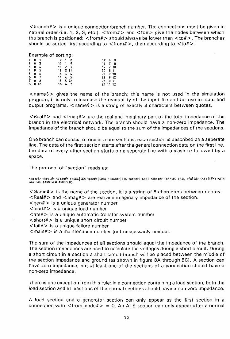
<branch#> is a unique connection/branch number. The connections must be given in natural order {i.e. 1, 2, 3, etc.). <from#> and <to#> give the nodes between which the branch is positioned; <from#> should always be lower than <to#>. The branches should be sorted first according to <from#>, then according to <to#>.
<name$> gives the name of the branch; this name is not used in the simulation program, it is only to increase the readability of the input file and for use in input and output programs. <name$> is a string of exactly 8 characters between quotes.
<Real#> and <I mag#> are the real and imaginary part of the total impedance of the branch in the electrical network. The branch should have a non-zero impedance. The impedance of the branch should be equal to the sum of the impedances of the sections.
One branch can consist of one or more sections; each section is described on a seperate line. The data of the first section starts after the general connection data on the first line, the data of every other section starts on a seperate line with a slash (!) followed by a space.
<Name$> is the name of the section, it is a string of 8 characters between quotes. <Real#> and <lmag#> are real and imaginary impedance of the section. < gen# > is a unique generator number <load#> is a unique load number < ats# > is a unique automatic transfer system number <short#> is a unique short circuit number <fail#> is a unique failure number <main#> is a maintenance number (not neccessarily unique).
The sum of the impedances of all sections should equal the impedance of the branch. The section impedances are used to calculate the voltages during a short circuit. During a short circuit in a section a short circuit branch will be placed between the middle of the section impedance and ground (as shown in figure 8A through 8C). A section can have zero impedance, but at least one of the sections of a connection should have a non-zero impedance.
There is one exception from this rule: in a connection containing a load section, both the load section and at least one of the normal sections should have a non-zero impedance.
A load section and a generator section can only appear as the first section in a connection with <from_node#> = 0. An ATS section can only appear after a normal
32
section.
There is no limit to the number of short circuits, failures or maintenance blocks in a section (apart from the memory limits of the computer).
A connection can consist of any number of normal sections. A section is a group of failures and short circuits that are repaired and maintained together. In other words: a section has a defined age. In a normal section any number of short circuits, any number of failures, and any number of maintenance blocks can occur, each with their own distribution for time-to-, occur and repair time, and each with the component after restore "as-good-as-new" or "as-bad-as-old".
4.2.2.2. A connection with a load section.
A connection with a load section consists of one load section (the first section) plus one ore more normal sections. No short circuits nor failures can occur in the load section. They can however be included in the normal section that has to follow the load section. A connection with a load section always originates from ground (node number 0)
A connection with a generator section consists of one generator section (the first section) plus possibly one or more normal sections. A connection with a generator section always originates from ground (node number 0)
A connection with an ATS section consists of one or more normal sections followed by an ATS section possibly followed by one or more normal sections. The ATS section can posses short circuits, fails and maintenance just like a normal section. The short circuits appear at the low_node side of the switch (ct. 3.8).
I '30kV cbl' 0.000 0.000 NSEC SHRT 4 FAIL 0 MAIN 0 ASGDNEW I 'transfor' 0.010 0.420 NSEC SHRT 5 6 FAIL 0 MAIN 0 ASGONEW I '1DkV cbl' 0.000 0.000 NSEC SHRT 7 FAIL 0 MAIN 0 ASGONEW I 'CirBr-171 0.000 0.000 NSEC SHRT 8 FAIL 0 MAIN 1 ASGDNEW
4 7 8 'switch23' 0.000 0.002 'cable 1 0.000 0.001 NSEC SHRT 9 FAIL 0 MAIN 0 ASGDNEW I 'switch 1 0.000 0.000 ATS 1 SHRT 10 FAIL 0 MAIN 1 ASGONEW 2 ASBDOLD I 'dummy 1 0.000 0.000 NSEC SHRT 11 FAIL 0 MAIN 2 ASGDNEW I 'cable 1 0.000 0.001 NSEC SHRT 12 FAIL 0 MAIN 0 ASGDNEW
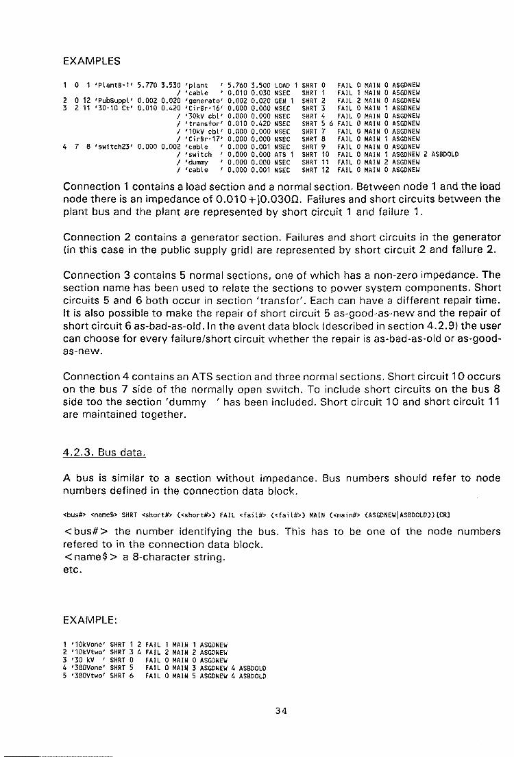
Connection 1 contains a load section and a normal section. Between node 1 and the load node there is an impedance of 0.010 + j0.0300. Failures and short circuits between the plant bus and the plant are represented by short circuit 1 and failure 1.
Connection 2 contains a generator section. Failures and short circuits in the generator (in this case in the public supply grid) are represented by short circuit 2 and failur~ 2.
Connection 3 contains 5 normal sections, one of which has a non-zero impedance. The section name has been used to relate the sections to power system components. Short circuits 5 and 6 both occur in section 'transfor'. Each can have a different repair time. It is also possible to make the repair of short circuit 5 as-good-as-new and the repair of short circuit 6 as-bad-as-old.ln the event data block (described in section 4.2.9) the user can choose for every failure/short circuit whether the repair is as-bad-as-old or as-goodas-new.
Connection 4 contains an ATS section and three normal sections. Short circuit 10 occurs on the bus 7 side of the normally open switch. To include short circuits on the bus 8 side too the section 'dummy ' has been included. Short circuit 10 and short circuit 11 are maintained together.
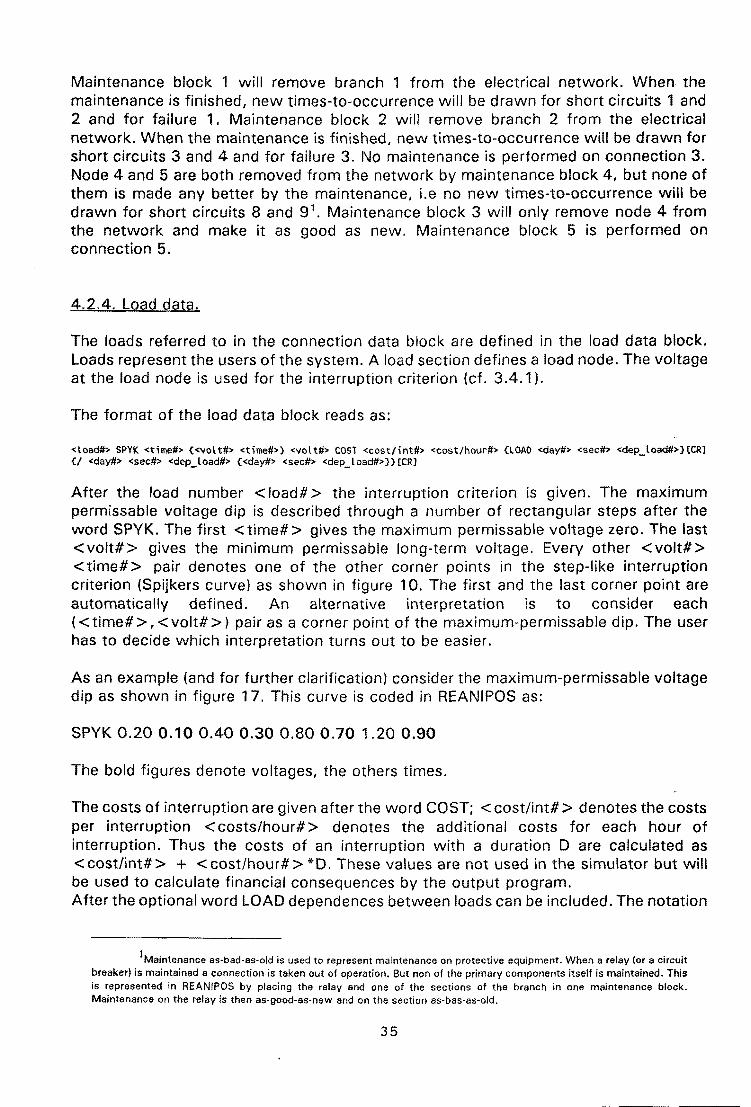
4.2.3. Bus data.
A bus is similar to a section without impedance. Bus numbers should refer to node numbers defined in the connection data block.
<bus#~ <name$> SHRT <short#> {<short#>} FAll <fail#> {<fail#>} MAIN {<main#> {ASGDNEWJASBDOlD}}[CR]
<bus#> the number identifying the bus. This has to be one of the node numbers refered to in the connection data block. <name$> a 8-character string. etc.
Maintenance block 1 will remove branch 1 from the electrical network. When the maintenance is finished, new times-to-occurrence will be drawn for short circuits 1 and 2 and for failure 1. Maintenance block 2 will remove branch 2 from the electrical network. When the maintenance is finished, new times-to-occurrence will be drawn for short circuits 3 and 4 and for failure 3. No maintenance is performed on connection 3. Node 4 and 5 are both removed from the network by maintenance block 4, but none of them is made any better by the maintenance, i.e no new times-to-occurrence will be drawn for short circuits 8 and 9 1
• Maintenance block 3 will only remove node 4 from the network and make it as good as new. Maintenance block 5 is performed on connection 5.
4.2.4. Load data.
The loads referred to in the connection data block are defined in the load data block. Loads represent the users of the system. A load section defines a load node. The voltage at the load node is used for the interruption criterion (cf. 3.4.1 ).
After the load number <load#> the interruption criterion is given. The maximum permissable voltage dip is described through a number of rectangular steps after the word SPYK. The first <time#> gives the maximum permissable voltage zero. The last <volt#> gives the minimum permissable long-term voltage. Every other <volt#> <time#> pair denotes one of the other corner points in the step-like interruption criterion (Spijkers curve) as shown in figure 10. The first and the last corner point are automatically defined. An alternative interpretation is to consider each (<time#>, <volt#>) pair as a corner point of the maximum-permissable dip. The user has to decide which interpretation turns out to be easier.
As an example (and for further clarification) consider the maximum-permissable voltage dip as shown in figure 17. This curve is coded in REANIPOS as:
SPYK 0.20 0.10 0.40 0.30 0.80 0.70 1.20 0.90
The bold figures denote voltages, the others times.
The costs of interruption are given after the word COST; < cost/int# > denotes the costs per interruption <costs/hour#> denotes the additional costs for each hour of interruption. Thus the costs of an interruption with a duration D are calculated as <cost/int#> + <cost/hour#> *D. These values are not used in the simulator but will be used to calculate financial consequences by the output program. After the optional word LOAD dependences between loads can be included. The notation
1Maintenance as-bad-as-old is used to represent maintenance on protective equipment. When a relay (or a circuit breaker) is maintained a connection is taken out of operation. But non of the primary components itself is maintained. This is represented in REANIPOS by placing the relay and one of the sections of the branch in one maintenance block. Maintenance on the relay is then as-good-as-new and on the section as-bas-as-old.
35
1.2~-----------------------------------,
:;; c. c
1 -
0.8 1- • • • . . • • • • • • • • • • • •
·; 0.6-. Cll .. ... 'j
0.4 1- .•
0.2 r-.
oL-~~--~--~----~--~--~ 0 0.4 0.8 1.2 1.6 2
time in seconds
Figure 17. Example of interruption criterion.
LOAD <day#> <sec#> <dep_load#> means that <dep_load#> will experience an interruption if the interruption of <load#> has a duration longer than <day#> days and <sec#> seconds. The first dependent load is described on the first line, every other line can contain one more dependent load.
7 SPYK 2.5 0.9 COST 0.0 0.0 LOAD 0.0 1.0 5 I 0.0 1.0 6 I 0.0 7200.0 4
I 0.0 7200.0 4
Loads 1, 2 and 3 can withstand a voltage zero for maximum 300 ms, a voltage of 70% for 1 second and a voltage of 90% for a long period. If one of these three loads experiences an interruption, so will the other two.
Load 4 experiences an interruption if the voltage at the load node is below 90% for longer than 200 milliseconds or if load 5, 6 or 7 experiences an interruption for longer than 2 hours (7200 seconds).
The loads 5, 6 and 7 experience an interruption if the undervoltage criterion of one of them is violated.
36
4.2.5. Generator data.
The generators referred to in the connections data block are defined in the generator data block. The generator data has the following format:
<gen#> <volt#> <angle#>[CRJ
After the generator number the voltage at the generator bus (in p.u) and the phase angle of the voltage (in degrees) are given. The phase angle is only needed in case two or more generators are present in the system.
EXAMPLE:
1 1.010 0.0 2 1.035 5.0 3 1.035 -3.0
4.2.6. Automatic transfer system data.
The automatic transfer systems (cf. 3.8) referred to in the connection data block are defined in the ATS data block. Its format reads as:
After the number of the ATS < ATS# > the reaction time <time#> in seconds is given. After the word FAIL a reference to the event definitions in the event data block is given. This denotes dormant fail-to-close of the ATS.
If the ATS is not in a dormant fail-to-close state it will close <time#> seconds after one of the branches <branch#> or one of the nodes <node#> is removed from the electrical network.
4.2.7. Short circuit data.
The short circuit data block relates the short circuits appearing in the connection data block to events in the event data block. The short circuit block further defines the operation of the protection by using a protection tree (cf. 3.6). The protection tree links the short circuit to one or more relays that might intervene to remove the short circuit. The relays are defined in the relay data block.
The format of the short circuit data block reads as:
The relay <rei#> will intervene <time#> seconds after the short circuit with a probability given by < dist# > ( < dist# > '¢ 0 } . Apart from this probability of non-
37
intervention the relay might be in a dormant fail-to-trip state. Also in that case it will not intervene. If < ats# > is closed the protection will be taken over by relay < ATSrel# >. It will intervene < ATStime# > after the short circuit with a probability given by <ATSdist#>. The ATS <ats#> will be opened <day#> days and <sec#> seconds after the intervention by < ATSrel# >. At that instant the branches and nodes removed by <ATSrel#> will be inserted again (cf. 3.8).
A line starting with BACKREL without the slash (!) is considered to be a continuation of the previous line. This is to enable the use of simple text editors to create the input file.
The operation of the protection with primary relays, backup relays, backup relays to backup relays etc. is modelled as a tree, like the one shown in figure 18. The first layer consists of the primary relays; the second one of the backup ~ relays, the third one of the backup relays to the backup relays, etc.
When a short circuit occurs the primary relays (denoted by PRIREL) intervene with a given probability. If one of them fails and it possesses a backup relay this backup relay will intervene with its probability. The process stops untill all
relays either intervene or do not possess Figure TB: Example of protection tree. a backup. The fault clearing time is then taken equal to the longest relay reaction time. At the instant of fault clearing the low-impedance branch at the fault position is removed and so are all branches and nodes belonging to the intervening relays. These branches and nodes are linked to the relays in the relay data block.
The relays in the first layer are denoted by the word PRIREL, those in the other layers by the word BACKREL. The nodes are given in the short circuit data block in a depth first way. The first line of data gives the upper branch of the tree. The number of slashes (/) at the start of the next lines denote the layer at which a new branch originates. One slash denotes a branch originating at the first layer; two slashes the second layer etc. For the tree of figure 18 this leads to the following data structure (relay data is omitted for clarity).
1 FAIL 1 PRIREL 1 BACKREL 2 BACKREL 3 BACKREL 4 I I BACKREL 5 BACKREL 6
After the relay number <rei#> a reference to the event data block for mal-trip is given followed by one for dormant fail-to-trip. <fail#> = 0 implies that this type of relay failure does not occur. After the word MAIN one or more maintenance blocks can be referred to, all of them with a choice between maintenance as-good-as-new or as-bad-asold; <main#> = 0 implies no maintenance. The branches and/or nodes that are removed from the electrical network when the relay intervenes, are given after the word BRANCH and RAIL, respectively. <branch#> = 0 implies that the relay has no influence on the network. Such a relay turned out to be useful e.g. to describe the behaviour of the protection with an ATS being closed.
Relay 1 shows mal-trip as well as dormant fail-to-trip; relay 2 only dormant fail-to-trip and relay 3 only mal-trip. In case relay 1 intervenes (either correct or incorrect) it removes branch 4 from the electrical network; relay 2 removes branch 8, relay 3 node 5. Relay 4 does not fail. It removes 4 branches and 4 nodes from the network. Such a relay
39
is often used as a final backup (sometimes called "disaster relay") that isolates all generators from the system in case all other backups fail. Also relay 5 does not fail. It even does not intervene in the network. Such a relay is used as a "dummy relay" to implement an ATS relay without a counterpart that reacts if the ATS is open.
4.2.9. Event data.
The event data block contains all the events referred to in the connection data block, in the bus data block, in the ATS data block, in the short circuit data blocl<, and in the relay data block. In those blocks one has to make sure that every fail number only appears once and that all numbers from 1 to the highest used value are present.
After the failure number <fail#> two references to distributions are given: the first one (preceded by the word DIST) denotes the distribution for the time to failure, the second one (preceded by the word REP DIST) denotes the distribution for the time to repair. The repair can be as-good-as-new (ASGDNEW) or as-bad-ad-old (ASBDOLD). The references to the distributions do not have to be unique, i.e. one distribution definition can be used for more than one event. The distributions are defined in the distribution data block.
The code DIST 0 implies that this failure event will not occur by itself. It may however occur as part of a common-mode failure. In the latter case the repair time distribution should have a reference to an existing distribution.
The maintenance data block defines the maintenance blocks referred to in the connection data block, in the bus data block, and in the relay data block. In those blocks one has to make sure that all maintenance numbers from 1 to the highest used value are present.
The format of the maintenance data block reads as:
After the maintenance number <main#> two references to a distribution are given each preceded by the word DIST. The first number refers to the distribution for the time-tomaintenance, the second one to the distribution for the duration of maintenance. The
40
end of the lines determines under what circumstances the maintenance is postponed. MTYPEO denotes that this maintenance is never postponed; MTYPE1 that this maintenance is postponed if it would lead to an interruption for one or more loads; MTYPE2 that this maintenance is postponed if another maintenance block is active; MTYPE3 denotes that the maintanance is postponed if one of the given branches or nodes is out of operation. If maintenance cannot be performed it is postponed until the objection against it is no longer present.
Maintenance block 1 is is always performed at the scheduled time, no matter what happens. Maintenance block 2 is postponed if it would lead to an interruption (e.g. maintenance on a parallel connection where one connection is out of operation for repair). Maintenance block 3 is performed if no other maintenance block is active. Maintenance block 4 is only performed if both branch 3 and branch 4 are present in the network. Maintenance block 5 is postponed if node 1 is not present.
4.2.11. distribution data.
The distribution data block defines the distributions referred to in the short circuit data block, in the event data block and in the maintenance data block. The format of the distribution data block reads as:
After the number of the distribution the type of distribution is given: WEIB denotes a weibull distribution with characteristic time <time#> days, shapefactor <shape#> and shift <min#> days;
BATH denotes a bath tub with a failure rate being the sum of three weibull distributions with characteristic times <time 1 # > days, < time2# > days and < time3# > days and shape factors <shape 1 # >, < shape2# > and < shape3# >. All three distributions are shifted <min#) days.
NORM denotes a normal distribution with expected value <mean#> days and standard deviation <st dev#> days. The minimum value of the distribution is <min#> days.
UN IF denotes a uniform distribution between <min#> days and <max#> days.
CHAN denotes a probability of <percent#> %.
41
4.2.12. connection dependency data.
In the connection dependency data block one can define ann out of k system. A branch will be removed from the electrical network if some other branches are no longer present in the network. The format of the connection dependency data block reads as:
<branch#> I <branch1#> <day1#> <sec1#> (I <branch2#> <day2#> <sec2#>}[CRJ
The branch denoted by <branch#> will be removed from the electrical network if branch <branch 1 # > is not present for <day 1 # > days plus <sec 1 # > seconds AND branch <branch2#> is not present for <day2#> days plus <sec2#> seconds AND etc.
EXAMPLE:
*Connect.dep 17 I 19 0.0 3600.0 I 20 0.0 3600.0 19 I 17 0.0 3600.0 I 20 0.0 3600.0 20 I 17 0.0 3600.0 I 19 0.0 3600.0
If two of the three connections 17, 19 and 20, are not present during one hour, the third one will be removed. It will be inserted again as soon as one of the two other branches is back in the network.
4.2.13. Common-mode failure data.
In the common-mode data block fail events, as defined in the event data block, are linked to each other. If an event occurs there will be a specified probability that some other event occurs after a certain time. The format of the common-mode failure data block reads as:
<fail#> I <fail#> <day#> <sec#> DIST <dist#> (I <fail#> <day#> <sec#> DIST <dist#>}[CRJ {/<fail#> <day#> <sec#> DIST <dist#> (I <fail#> <day#> <sec#> DIST <dist#>}[CR]}
If the first failure occurs, the others will occur after the given time (<day#> days plus <sec#> seconds) with the probability defined by < dist# >. DIST 0 implies a probability of 100%. Every failure can have an unlimited number of common-mode failures, but each line of data can only contain two.
The common-mode failure is repaired as soon as the original failure is repaired.
By using this common-mode failure one can link any short-circuit, section failure, bus failure, failure of ATS or relay failure to any other short-circuit, section failure, bus failure, failure of ATS or relay failure.
Maintenance events are not treated as failures so they cannot be linked to other events.
42
4.2.14. End of data.
The end of the input data reads as:
.END
Everything after this end of data sign is not read by the simulator. One might however use this to store data for other purposes (i.e. for use by an input or output program).
4.3. The output file.
The output file of REAI\IIPOS contains information about the events that took place during the simulation. The user can choose between normal output (only data about start and end of interruptions) end extended output (data about QJl events).
Warning: when using the extended output option the output file can easily become several Mega Bytes large. The user has to make sure that there is sufficient space on the disk. An easier way to get some detailled information is to sent the extended output data of the last period or of some of the last periods to the printer.
The first line of the output file contains the duration of one period in days. Next follows one line for each load present, containing the load number, the costs per interruption, the costs per hour of interruption and the load name.
EXAMPLE
10950.000 1 1.000 2 10.000 .DATA
10.00 0.50
plant A plant B
After the word ".DATA" follows the event data.
In case of normal output each line contains: period number; day and second of event; status for each load ( 1 = no interruption; 0 = interruption).
This means that in period one an interruption for load one started after 3347 days and 75846.65 seconds (i.e. after 9 years and 2 months) and ended after 3349 days and 25276.70 seconds. The interruption of load 2 started 0.01 sec. after that of load 1.
In case of extended output each event line (of which there are many more now) also contains the voltage at each of the load nodes, the current event and the current system state.
43
The following abreviations are used for the events:
FA# = Failure # MA# = start maintenance block # RE# = intervention by relay # ER# = end of repair # EM# = end of maintenance block #
The following abbreviations are used for the state:
BR# = branch # has been removed from the electrical network RL# = node # has been removed from the electrical network RS# = relay # is in a dormant fail-to-trip state AS# = A TS #is in a dormant fail-to-close state AT# = ATS #is closed SH# = short circuit # is present in the electrical network
The same event has been given as before, but now more information is available. One can see that failure 14 (=short circuit 4) occurs followed 0.2 seconds later by an intervention of relay 6 leading to the removal of branch 5, branch 6 and bus 1 from the electrical network. Plant one experiences an interruption 0.65 seconds after the relay intervention, plant 2 0.01 second later. Because of the interruptions branch 12 and 13 are removed. About two days later all branches are inserted again due to the end of repair and the system gets back to its normal state.
4.4. The REANEDIT input program.
The REANEDIT program is fully menu driven. It is intended to be much more user friendly than the input file of the REANIPOS simulator. The following main menus are present: - the file menu; - the structure menu; - the voltage menu; - the reliability menu.
Only those menu parts that are accessable at a certain moment are highlighted. In this way the user is forced to follow a certain path. The normal input session will follow the consecutive submenus starting from the structure menu. Going back to an earlier submenu, often means going through all other submenus as well. The data is however not lost, and the submenus can be passed fast.
The functions of the four menus and their submenus will be briefly discussed below.
44
4.4.1 . The file menu.
Within the file menu the following options are present: * to printer: output of the current file to printer {i.e. the REANVIEW output file which
serves as the REANIPOS input file). This option also works if the input session is not yet finished. It turned out that a fast overview of the system can be obtained from reading the file if some basic knowledge of the filets structure is present. This is faster than passing through all the REANEDIT menus. The user is recommended to set the printer to a small letter type.
* to screen: output of the current file to screen. * save: saving the file on disk. This option also works if the input session is not yet
finished. The user can continue the input session at a later instant. * load: loading a file from disk. This is to continue an interrupted input session or to
make some changes in the system. * new: erase current system and start with a clean one. The program will not
automatically save the file. * quit: leave REANEDIT.
4.4.2. The structure menu.
Within the structure menu the user builds the electrical network: i.e. the different branches and sections plus their impedances. Also the positions of loads/ generators and automatic transfer systems are determined. The user can also give names to branches/ sections and nodes. These are used as reference during the rest of the input session.
Before starting an input session the user has to define the node numbers. These will not change during the input session/ unless nodes are removed. The numbering of the branches is done by REANEDIT.
Within the structure menu the following options are available: * common data: input of simulation name; frequency; base power; base voltage;
random seed; period length (life time); and permissable error. * branch data: adding of branches to the electrical network and changing of branch
data. Each branch is divided in a number of sections. For each section the impedance and the section type has to be given. For the section type one can choose between "normal section" I "load section" I "generator section"/ and "ATS section". The user can give a name to every section and to every branch. Although these names do not have to be unique/ the user is recommended to use easyly recognizable unique names. This will prevent a lot of searching further on in the input session. The branch data screen contains a window with a list of all branches that are present in the system. The following options are present: * * edit sections: edit the data of existing sections of the branch indicated in the
window. The screen will show the data of one section. The user can change the section data/ insert a section before or after the section shown and delete the section. By using the options previous and next the user can chooose another section.
* * rename branch: change the name of the indicated branch. Changing a section name is done by the edit sections option.
* * add branch: add a new branch to the network (a new connection to the system).
45
Both node numbers have to be given plus the impedance and type for one section. To include more sections the user has to choose the edit sections option. The program will renumber the connections after a new connection has been included.
* * delete branch: remove the indicated connection from the network. The program will renumber the branches after a connection has been removed from the system.
* * bacl<: return to main menu.
* rail data: changing the bus names and removing busses. In the latter case the corresponding node plus all branches connected to this node are removed. This is an easy tool to remove large parts of a system, but also very dangerous for one might loose a large amount of data by pressing one key. Like with the branches and sections the user is recommended to use easyly recognizable unique names for the busses. A window shows all busses present in the system. The following options are available: * * delete rail: remove the indicated node from the network. Remind that all
branches connected to this node are also removed. * * rename rail: change the name of the indicated bus. * * back: return to the main menu.
* structure test: after inputting the branch and bus data a structure test has to be performed. It tests whether all branches have a non-zero impedance, whether load, generator and ATS sections are used correctly, and if the electrical network forms one coherent structure (i.e. all generators are connected to all load nodes).
4.4.3. The voltage menu.
In this part of the program the user has to input the data for the generator, load and ATS sections. These sections have been introduced already in the branch data submenu.
Within the voltage menu there are the following possibilities. * generator data: input generator voltage and calculate node voltages to determine the
generator voltage wanted. The screen contains a window showing all generators present in the system. The following options are present: * * edit generator: change amplitude and angle of the voltage of the indicated
generator. * * rail voltage: show voltages at all user defined nodes. * * load voltage: show voltages at all load nodes. ** bacl<: return to main menu.
* load data: input interruption criterion; dependent loads; and costs of interruption. The screen contains the data for one load at a time. The options next and previous enable the user to see and edit the data of other loads. The screen shows a window with all dependent loads and a window with all (time-voltage) points of the interruption criterion. Fields are present for the costs per interruption and the costs per interrupted hours. The following options are available: * * add dependent load: pick a new dependent load from a list of loads. * * delete dependent load: remove the indicated dependent load.
46
* * add under voltage: add a point to the interruption criterion curve. * * delete under voltage: remove the indicated point from the interruption criterion
curve. * * back: return to main menu.
* ATS data: input reaction time of ATS and branches/nodes whose removal leads to closure of the ATS. The screen shows the ATS time and windows for the nodes and the branches influencing the ATS. Only the data for one ATS is shown in the screen. The options next and previous enable the user to see and edit the data of other ATS's. The following options are further present: * * add rail: make the ATS dependent on a node. The node can be picked from a list
of all nodes available. * * delete rail: remove the indicated bus from the list. * * add branch: make the ATS dependent on a branch. The branch can be picked
from a list of all branches available. * * delete branch: remove the indicated branch from the list. * * back: return to the main menu.
* voltage test: test to determine if the normal state load node voltages are high enough in comparison to the interruption criterion.
4.4.4. The reliability menu.
In this part of the input program the user is going to introduce disturbances in the system: relays are introduced; short circuits plus their protection trees; other failures; distributions for time-to-fail and for time-to-repair and maintenance blocks.
Within the reliability menu the following options are available: * relay data: The relays have to be numbered by the user. This numbering is important
because it is used for the protection trees. The user is suggested to make a drawing of the power system with the relays included before the input of the protection trees. For each relay one or more branches and/or nodes can be given that are removed from the electrical network if the relay (correctly or incorrectly) intervenes. The screen shows the data for one relay only. The options next and previous enable the user to see and edit the data of other relays. The branches and nodes linked to the relay are shown in two windows on the screen. The following options are further available: * * add rail: add a node to the list of nodes removed from the system if the relay
intervenes. The user has to pick this node from a list of available nodes. * * delete rail: remove the indicated node from the list. * * add branch: add a branch to the list of branches removed from the system if the
relay intervenes. The user has to pick this branch from the list of available branches.
* * delete branch: remove the indicated branch from the list. * * add relay: add a new relay to the list of relays. The relay is included before or
after the relay shown on the screen. The user has to keep in mind that adding a new relay before another one changes the numbering.
* * delete relay: remove the relay shown on the screen from the list of relays. This will change the numbering of part of the other relays.
47
* * bacl<: return to main menu.
* short circuit data: input the position of the short circuits plus the corresponding protection trees. For the position of the short circuit the user can choose from a list of all suitable sections. After a short circuit is placed in the system the user has to input the protection tree. This turned out to be one of the most difficult parts of the input session. The user is recommended to draw the power system with the relays and all protection trees beforehand and to check the protection trees in the file by using the drawing of the power system. All short circuits present are shown in a window on the screen. The following options are present: * * add short circuit: add a new short circuit to the system. The user has to choose
from a list of all possible positions for the short circuit (i.e. all suitable nodes and sections).
* * delete a short circuit: remove the short circuit indicated in the window from the system.
* * edit short circuit: change the protection tree if present; create the protection tree if not yet present. The protection tree is shown in a window on the screen. The data at the indicated position in the tree is shown under the window. The normal relay as well as the A TS relay can be edited. If the fields for the ATS relay are empty, there is no ATS relay present. The data under the window can be edited. In this screen the following options are available: * * * up: move the indicated position one step upwards in the protection tree.
If this action is not possible the indicated position will not move. * * * down: move the indicated position one step downwards in the protection
tree. * * * left: move the indicated position one step leftwards in the protection tree. * * * right: move the indicated position one step rightwards in the protection
***
***
***
tree. add relay: add a relay parallel to or as a backup for the indicated relay. This option is not for all positions in the tree available. delete relay: delete the indicated relay from the tree. In some cases it is only possible to remove more than one relay. The user will automatically note this. back: go back to the short circuit data screen.
* * back: return to the main menu.
* failure data: input of distributions for uptime and downtime; input of failures of sections, relays and automatic transfer systems. The failures belonging to the short circuits are automatically generated, the others have to positioned by the user. The user can thereby choose from a list of all available failures. The screen shows the data for one failure at a time. The options next and previous enable the user to see and edit the data of other failures. The following options are further present: * * add failure: add a new failure to the system. The user has to choose from a list
of all possible failures of sections, relays and ATS's. * * delete failure: remove the failure shown on the screen from the system. * * edit failure: define or change the distribution for the time to failure. * * edit repair: define or change the distribution for the time to repair.
48
* * toggle repair type: change repair from as-bad-as-old to as-good-as-new or vise versa.
* * back: return to main menu.
* maintenance data: input of maintenance blocks and distributions for time to maintenance and duration of maintenance. The data for one maintenance block is shown on the screen. The options next and previous enable the user to see and edit the data of other maintenance blocks. The following options are further present: * * Edit maintenance: change the conditions under which the maintenance block is
postponed. * * add maintenance: create a new maintenance block. * * delete maintenance: remove the maintenance block shown on screen from the
system. * * toggle maintenance type: change maintenance type from as-bad-as-old to as
good-as-new or vice-versa. * * distribution data: define or change the distributions for the time to maintenance
and for the duration of maintenance. * * add components: add components to the maintenance block. The user can
choose from a list of maintainable components. * * delete components: remove the indicated component from the maintenance
block. * * back: return to main menu.
* maintenance and failure test: some final tests. If these tests are passed the file is ready for the REANIPOS simulator.
4.5. The REANVIEW output program.
The output program REANVIEW enables the user to create graphical and other output from the REANIPOS output file. The program can generate the following functions: - expected number of interruptions per year; - expected costs per year; - probability density of number of interruptions per period; - probability density of costs per period; - probability density of duration of interruption.
The user can choose between: - a graphical presentation on screen; -a graphical presentation on printer (epson matrix or HP laserjet); - an HPGL file of the graphical presentation; - a table to printer; - a table to file.
The program can further calculate the following parameters for all loads and send them to printer: - expected number of interruptions during one period; - expected costs during one period; -expected interrupted hours during one period.
For more details about the REANVIEW output program please refer to [11 ].
49
Chapter 5: examples.
5.1. Influence of repair-time distribution on non-availability of a parallel system.
In a reliability study of a district heating system, the negative-exponential distribution has been used for the time-to-repair. After a presentation of this study there was a short discussion about the possible influence of the repair-time distribution on the availability of the system. We decided to use REAI\IIPOS to quantify this influence.
In the system under consideration the components had a failure rate of 8 y(1 and an average repair time of 25 hours.
The following REANIPOS model has been used for this: * two parallel connections with a low impedance; each consisting of one section
* *
*
with one "failure"; one source connection with a low impedance generator section; one sink connection with a high impedance load section and a low impedance normal section; both failures posses an exponential distribution for the time-to-failure with an expected time of 50 days, and a Weibull distribution for the time-to-repair with an expected repair time of 1 day.
As REANIPOS uses the characteristic time 8 as an input parameter for the Weibull distribution, it had to be calculated from the expected time E(T) by using:
1 E(T) = 6 P(l+-) m
where r is the gamma function and m the shape factor. By using a table for the gamma function we found the following values for the characteristic time to repair in days:
m = 1 8 1.000 m = 3 8 = 1.120 m = 5 8 = 1.089 m = 7 8 = 1.069 m = 9 8 = 1.056
shape number inter. hours per factor of inter. hours inter.
As reliability parameters we choose for the expected number of interruptions per 10 years and the expected number of interrupted hours per 10 years. We performed simulation for different values of the shape factor of the repair time distribution. The results are given in the table above. Each row is the result of the simulation of 10,000 periods of 10 years. The last column gives the expected duration of one interruption.
Figure 19 shows the trend. We see that the expected number of interruptions is independent of the shape factor whereas the expected number of interrupted hours slightly increases with increasing shape factor. The influence is however only small. Our conclusion is therefore that the exponential distribution (m = 1) is an acceptable approximation.
Figure 20 shows the duration of interruption for the m = 1 case; figure 21. for the m = 9 case. The influence on the distribution is clear, but the average length is not influenced by the repair time distribution. By comparing figures 20 and 21 can conclude that the reliability/availability will be influenced by the repair time distribution in case an interruption starts to become important after a couple of hours. We therefore performed another round of simulations (5 times 10,000 periods of 10 years) to
Figure 19. Influence of repair time distribution on reliability and availability of a parallel system.
quantify this influence. In this case we counted an interruption only as an interruption if it's duration would be longer that 3 hours (in REANIPOS language: the plant can withstand a voltage zero for 3 hours). The results are presented in the table below and in figure 22.
o. a2. 65. Z7. 71 o. 82. re.m.ao.Z3.25J!B.30.33.!i5.l8. f't. 4:3.'95.1B.fl1.'i* .!lo.\19.61 M .d7 .m.<:2.:z.t :n .33J!!I2.86.S7 .:i!.O.~.S5.s:>. s
Figure 20. Probability density function of duration of interruption for an exponential distibution for the time-to-repair. The horizontal scale reaches from 0 to 100 hours.
Figure 21. Probability density function of duration of interruption for a Weibu/1 distribution with a shape factor of 9 for the time-to-reapir. The horizontal scale reaches from 1 to 27 hours.
numbers hours
3 30
+ 2.5 + + 25 .
2 20
• number of inter.
1.5 15 + hours per period
* hours per inter 1 10
0.5 5
0 0 1 2 3 4 5 6 7 8 9
shape factor
Figure 22. Influence of shape factor on reliability parameters for interruptions longer than 3 hours.
5.2. Influence of voltage solidity.
Consider the power system shown in figure 23: two 10 kV plant busses, each connected by two transformer links to a 30 kV substation fed from the 150 kV network. The links are protected by differential relays, with over-current time relays serving as a back-up. The over-current time relays will, in general, also protect the plant busses. In this example we will assume that only short circuits in the transformer links can occur. The over-current time relays are assumed to be fully reliable, whereas the differential relays can fail.
Figure 24 shows the voltage shape at plant bus A for 4 situations: A: a short circuit in the connection to plant A, disconnected by the differential relay; ~: the same short circuit disconnected by the over-current time relays (i.e. when the differential protection fails); C: a short circuit in the connection to plant B, disconnected by the differential relay; D: the same short circuit disconnected by the over-current time relays.
The design of the power system will, normally, be such that the plant can withstand voltage dips A and C (if not, it is of no use having two links in parallel). In case of situation B, plant A will certainly experience an interruption, in case of situation D probably.
The system as modelled in REANIPOS is shown schematically in figure 25 wher the rectangles represent connections, the thick horizontal lines busses; the circles short circuits; and the squares relays. Relays 1, 2, 5 and 6 represent differential relays; 3, 4, 7 and 8 over-current time relays.
54
150kV
PLANT B
PLANT A
Figure 23. Redundant supply to two plants.
Volt Volt f- f-
I A . B .
time time
- - - - - - - -
Volt Volt 1--f-
c D
time time
Figure 24. Voltage dips experienced by plant A in figure 23.
Figure 25. Redundant supply to two plant (ct. figure 23) modelled in REANIPOS,.
The following protection trees are used in the REANIPOS model:
SHORT1L2, 0.2s, 1oo%L3, 0.6s, 100% 4, 0.6s, 100%
1, 0.2s, 5%
SHORT2L1, 0.2s, 1oo%L3' 0.6s, 100% 4, 0.6s, 100%
2, 0.2s, 5%
SHORT3L6, 0.2s, , 0.6s, 100% , 0.6s, 100%
5, 0.2s, 5%
SHORT4L5, 0.2s, 1oo%L1, 0.6s, 100% 8, 0.6s, 100%
6, 0. 2s, 5%
In words: the short circuit is to be removed by the differential relay in the faulted link. If this one is dormant the over-current time relays in both links will intervene. The differential relay in the non-faulted link has a 5% change of mal-trip.
The following component data have been used: * a short circuit in a 30/1 0 kV link is expected to occur once every 1 0 years; * no other short circuits occur; * the differential relay's time-to-occurrence for a "dormant fail-to-trip" has a Weibull
distribution with a characteristic value of 5 years and a shape factor of 3; * no other relay failures occur; * the plants can withstand the voltage dip due to a short circuit if the differential relay
clears it, but not if the over-current time relay clears it; * maintenance is performed exactly every 10 years during exactly 24 hours;
56
Drob. Dens. of It Int/Period ( in % }
7.52
3.76
0 2 3 5 7 8 9 10 11 12 13
Figure 26. Probability density function of the number of interruptions for the base case.
Figure 27. Expected number of interruptions per year, for the base case.
57
* a left-bounded normal distribution has been used for the repair time. The expected value, standard deviation and minimum value are 5 days, 3 days and 2 days, respectively, for the short circuit and 2.4 hours, 2.4. hours and 30 minutes, respectively for the relay.
The result of 400 simulations of 30 years, is given in figure 26 and figure 27. Figure 26 shows an estimation for the probability density function for the number of interruptions in 30 years. The estimation for the expected number of interruptions in 30 years is 4.5. As can be seen in figure 26 the number of interruptions shows a large spread; with about 90% certainty the value is between 2 and 9 interruptions per 30 years.
Figure 27 shows the system behaviour as a function of time. Initially (i.e. for small system age) an interruption of the supply is due to the simultaneous occurrence of a short circuit on two parallel connections or due to a mal-trip of the relay in the parallel connection. The corresponding failure rates are 0.0003 yr"1 and 0.01 yr"1
• The latter is clearly dominant. But gradually the chance that a differential relay is in the dormant failto-trip state increases. The system transfers from a redundant system to a nonredundant system in which every short circuit will lead to an interruption of the supply (the system transfers from a logical parallel connection to a logical series connection). The expected number of interruptions for the non-redundant system is 0.4 per year. After 10 years all relays are maintained and become as-good-as-new. The expected number of interruptions resets to its initial value and then gradually increases again.
Figure 28 and figure 29 show the results for an extremely sensitive load. It is assumed here that the plant cannot even withstand a voltage dip of 200 milliseconds (due to intervention by the differential protection). In that case every short circuit leads to an interruption of the supply. A failure of the primary protection will not be of influence any more, nor will maintenance. The expected number of interruptions equals 0.4 per year, thus 12 per 30 years. The number of interruptions in 30 years is, with about 90% certainty, between 8 and 20.
Figure 30 and figure 31 show the results for an extremely insensitive load: even a voltage dip of 600 milliseconds does not lead to an interruption. This implies a reduction of the number of interruptions by a factor of two, as compared to the base case. The estimated value for the expected number of interruptions in 30 years is 2.4. The number of interruptions is, with about 90% certainty, between 1 and 4.
58
Drob. OO?ns. or # InvDeriod ( in % )
13.5
10.8
8.12
5.41
2.71
-. 5 tS 7 a s 10 u 12 13 H 15 16 17 1a t9 20 21 22 23 21 25 26 27
Figure 28. Probability density function of number of interruptions in 30 years, for an extremely sensitive load.
0.25
0.12
1 2 3 -. 5 o 7 a s 10 11 12 13 11 15 16 17 ta 19 20 21 22 23 21 25 26 27 za 29 30 31
Figure 29. Expected number of interruptions per year, for an extremely sensitive load.
59
Prob. Dem;. of It InuDeriod ( in % ) fdbriek LoddNo :1
Figure 30. Probability density function of number of interruptions in 30 years, for an extremely insensitive load.
Figure 31. Expected number of interruptions per year for an insensitive load.
60
5.3. Influence of maintenance.
For the base case of the previous paragraph we varied the time to maintenance between 10 years and 0.5 years. Figures 32 through 34 show the expected number of interruptions for a time-to-maintenance of 5 years, 4 years, and 3 years, respectively. (Note the change in vertical scale.)
Figure 35 shows the expected costs of interruption during 30 years, as a function of the time-to-maintenance. The more often maintenance is performed, the lower the costs of interruptions. It has been assumed here that every interruption costs f20,000.- plus f20,000,- per hour, the recommended value for a 1 MW plant according to the IEEE Gold Book [8].
The expected number and costs of interruptions per 30 years as a function of the timeto-maintenance are given in the table below.
II years to main. number of inter. costs of inter.
' 10years 4.5 !6,700,000.-
i 7 years 3.3 f4,900,000.-
5 years 2.0 !3,200,000.-
4 years 1.3 f2,200,000.-
3 years 0.8 (1,500,000.-
2 years 0.5 f1,000,000.-
1 year 0.4 !1,000,000.-
0.5 years 0.4 f900,000.-
To determine the optimal time-to-maintenance the costs of maintenance should also be taken into account.
Figure 34. Number of interruptions when maintenance is done every 3 years.
7
6r
6
"' ~ 4 r-·e ., -;:; 3 r-0
(.)
.. 2
.. 1 a "' "
oL-----~I _______ L_I ____ ~-------L-1----~
0 2 4 6 s 10
years to maintenance
Figure 35. Influence of time-to-maintenance on the costs of interruption.
63
6. Acknowledgements.
The main responsible for the software in REANIPOS is Koen Verstappen. He also wrote the input program REANEDIT. The predecessors of REANIPOS, were written by master students in our group: Hans van Kempen, Roeland Cerfonteijn and Roland van de Vijver. The output program REANVIEW was written by Serban-Aiexander Stanasila.
Further assistance was obtained from Hans Voncken (DSM Limburg BV), Patrick Marteijn (Dow Benelux NV), Frank van der Duyn Schouten (Tilburg University) and from Wil van den Heuvel.
64
7. References.
[1] Diliberti, T.l. and V.E. Wagner, J.P. Staniak, T.O. Orloff POWER QUALITY REQUIREMENTS OF A LARGE INDUSTRIAL USER; A CASE STUDY. In: Industrial and Commercial Power Systems Technical Conference 1990. N.Y.: IEEE, 1990. P.1-4.
[2] McGranaghan, M. and D. Mueller, M. Samotyj VOLTAGE SAGS IN INDUSTRIAL SYSTEMS. In: Industrial and Commercial Power Systems Technical Conference 1991. N.Y.: IEEE, 1991. P.18-24.
[3] Koval, D.O. and J.J. Leonard, Z.J. Licksko POWER QUALITY OF SMALL RURAL INDUSTRIES. In: Industrial and Commercial Power Systems Technical Conference 1991 .. N.Y.: IEEE, 1991. P.78-83.
[4] Billinton, R. and R.N. Allan POWER SYSTEM RELIABILITY IN PERSPECTIVE. Electronics and Power, Vol.30 (1984), p.231-236.
[5] Kloeppel, F.W. STRUKTUR- UND FUI\IKTIONSZUVERLASSIGKEIT ALS ENTSCHIEDUNGSKRITERIEN FOR DIE QUALTITAT DER ELEKTROENERGIEVERSORGUI\JG. Energietechnik, Jg, 40 ( 1990), S.444-452.
[6] Fishman, G. and L. Moore AN EXHAUSTIVE ANALYSIS OF MULTIPLICATIVE CONGRUENTIAL RAI\IDOM NUMBER GENERATORS WITH MODULUS 231 -1. SIAM Journal of Scientific and Statistical Computing, Vol. 7 ( 1985), p.24-45.
[7] Verstappen, K.F.L. REANIPOS PROGRAM LISTING AND COMMENTS.
[8] IEEE recommended practice for the DESIGN OF RELIABLE INDUSTRIAL AND COMMERCIAL POWER SYSTEMS (IEEE gold book). N.Y.: IEEE, 1991. ANSI/IEEE Std. 493-1990.
[1 0] IEEE recommended practice of EMERGENCY AND STANDBY POWER SYSTEMS FOR INDUSTRIAL AND COMMERCIAL POWER SYSTEMS (IEEE orange book). N.Y.: IEEE, 1987. ANSI/IEEE Std. 446-1987.
[11] Stanasila, S.-A. REANVIEW: POSTPROCESSING TOOL OF THE REANIPOS PACKAGE. Eindhoven University of Technology, Group of Electrical Energy Systems, June 1992. Report EG/92/597.
[12] Box, G.E.P. and M.E. Muller A NOTE ON THE GENERATION OF RANDOM NORMAL DEVIATES. Annals of Mathematical Statistics, Vol. 29 (1958), p.61 0-611.