Reasoning About Secrecy for Active Networks Pankaj Kakkar University of Pennsylvania [email protected]Carl A. Gunter University of Pennsylvania [email protected]Mart´ ın Abadi [email protected]Abstract In this paper we develop a language of mobile agents called uPLAN for describing the capabilities of active (programmable) networks. We use a formal semantics for uPLAN to demonstrate how capabilities provided for programming the network can affect the potential flows of information between users. In particular, we formalize a concept of security against attacks on secrecy by an ‘outsider’ and show how basic protections are preserved in the presence of programmable network functions. 1 Introduction The goal of research on programmable or active networks [21, 20] is to make computer networks more flexible. This flexibility threatens the security of the network, so good techniques for modeling and analyzing the consequences of providing new network services are desirable. This paper describes an approach based on a simple language of mobile programs. The primary contributions are a definition of secrecy for a simple model of active networks and routing, an analysis of how this definition relates to one based on bisimulation, and a collection of case studies. Properties that Aid Scalability. The Internet has proved the value of high connectivity in networking. Active networking research has attempted to achieve scalability too, aiming to accommodate internetworks composed of thousands of physical networks, multiple administrative domains, and a diver- sity of users. However, some users may harbor ill-will towards others, or even towards the network as a whole. Even when no bad intentions are involved, a programmable network may be vulnerable to mistakes or unexpected inter- actions between its users. The mechanisms for programming the network may 1
In this paper we develop a language of mobile agents called uPLANfor describing the capabilities of active (programmable) networks. We usea formal semantics for uPLAN to demonstrate how capabilities providedfor programming the network can affect the potential flows of informationbetween users. In particular, we formalize a concept of security againstattacks on secrecy by an ‘outsider’ and show how basic protections arepreserved in the presence of programmable network functions.
1 Introduction
The goal of research on programmable or active networks [21, 20] is to makecomputer networks more flexible. This flexibility threatens the security of thenetwork, so good techniques for modeling and analyzing the consequences ofproviding new network services are desirable. This paper describes an approachbased on a simple language of mobile programs. The primary contributionsare a definition of secrecy for a simple model of active networks and routing,an analysis of how this definition relates to one based on bisimulation, and acollection of case studies.
Properties that Aid Scalability. The Internet has proved the value ofhigh connectivity in networking. Active networking research has attemptedto achieve scalability too, aiming to accommodate internetworks composed ofthousands of physical networks, multiple administrative domains, and a diver-sity of users. However, some users may harbor ill-will towards others, or eventowards the network as a whole. Even when no bad intentions are involved,a programmable network may be vulnerable to mistakes or unexpected inter-actions between its users. The mechanisms for programming the network may
1
also be helpful in damaging it. Such problems are not limited to new kinds ofprogrammable networks; the current Internet has problems of its own. Complexinteractions between features may lead to vulnerabilities in systems thought tobe well-understood. For example, Bellovin [7] showed how to combine remotelog-in, the domain name system (DNS) directory, router table updates, andother features to compromise Unix hosts on the Internet. Clearly the growth ofmobile agents has created new risks for hosts; programmable networks that aimto move this form of agent into routers bring additional risks and challenges.
Research on programmable networks has sought to address these concernsby a variety of mechanisms. One is to imitate features of the Internet that havecaused it to be scalable and survivable. A simple example is the way the Internetprotocol (IP) uses a Time-To-Live (TTL) field to limit the effects of routingloops. The TTL field also relates the ability of a host to affect the network tothe size of its attachment: a user with a modem is not able to send very manypackets in the first place, and the packets sent cannot circulate infinitely orcreate many new packets to waste bandwidth. Programming systems for activenetworks, generally known as Execution Environments (EE’s), often providesome analog of the TTL field to control network resource utilization.
The aim of this paper is to look at another form of protection that aidsthe usability and survivability of the Internet. In this paper we call it SecurityAgainst Outsiders or AO-security. The Internet has been able to survive thethreat of password sniffing, that is, the ability to listen to network traffic andfind passwords that can be used to gain illegitimate access to hosts or routers.Various protocols are available to avoid sending passwords in cleartext over thenetwork, but the use of cleartext passwords is still very common. A primaryreason is the fact that when a password is sent between one host and another,it does not visit every network in the Internet on the way. A party seekingto learn the password may not have an obvious mechanism for listening on anetwork if he does not have access through a host attached to it. While thepassword is vulnerable to sniffing by ‘insiders’ who are on the networks overwhich it will pass, it may be less vulnerable to ‘outsiders’ who must sniff fromafar with little toe-hold from which to grab and redirect the sensitive informa-tion. Protocols that enable internetwork routing systems to adapt to topologicalchanges such as router failures also cause packets to appear in unexpected placesin the network, so topological guarantees are generally viewed as a weak formof protection. However, topological guarantees are a recognized practical partof current protections against vulnerabilities like password sniffing and also pro-vide protections against more sophisticated attacks such as traffic analysis. Forexample, topological guarantees can make it harder to collect large amounts ofciphertext or determine whether an encrypted email was sent between two par-ties at a given time. AO-security is sometimes dumb luck; but it is often crucial,for example, in corporate networks behind firewalls and with moderate securityrequirements. The aim of this paper is to study AO-security in the context ofactive networks, where luck may not be enough. Our study provides insight intothe protection afforded by programming interfaces and physical topology.
2
The Challenge of AO-Security for Active Networks. When we allow anetwork to become programmable, some of the apparent AO-security enjoyed bythe Internet protocols may be lost if programmability of routers is available tooutsiders and the right kinds of operations are made available to them. For ex-ample, researchers in the SwitchWare Project at the University of Pennsylvaniahave experimented with downloadable OCaml modules capable of dynamicallyaltering switching and queuing strategies on routers [13, 6]. The privilege to usesuch a function will probably be limited by some form of cryptographic autho-rization system [5], but the underlying capabilities easily accommodate a man-in-the-middle attack on all of the packets passing through the affected router.Password sniffing would clearly be a possibility from any site that was able toobtain these capabilities. Execution environments like PLAN [14], ANTS [23],and others strive to control the tradeoff between security and flexibility by limit-ing the programming interface available to active network agents. This strategycan be applied quite flexibly. For instance, Hicks and Keromytis [12] describean active firewall where outsiders passing through are allowed to use active net-work capabilities but only on a limited interface available to ‘visitor’ packets. Inparticular, the firewall places wrappers on visitor packets that limit the symboltable of the packet when it evaluates on a router.
To realize the goal of understanding the limits of AO-security in active net-works we need to develop a theory for explaining the effect on security of offeringnew services on routers. Such an explanation is not only important to ‘purelyactive’ networks, but also to deployments of active network EE’s within theInternet, for instance in the ABONE (www.csl.sri.com/activate) active net-work testbed. Indeed, some of the examples we give below are meaningful tosome degree even for the current Internet, especially as moves are being madeto extend the capabilities of routers to include things like multicast, resourcereservation, and even web caching. The ability to reason about interactions be-tween routing and computation at endpoints may also be important as mobileagent technology progresses and connections between hosts and routers becomemore complex.
Requirements for a Suitable Theory. There are at least two problems thatmust be overcome in developing a suitable theory for relating router interfacesto AO-security in the network. First, it is necessary to develop a rigorous butsimple concept of secrecy. Second, it is essential to represent the techniquesin a sufficiently general way that the methods are applicable to more than oneprotocol or active network architecture.
Our approach to modeling secrecy is inspired by work on the spi calculus [2,4, 3], which uses ideas from concurrency theory to model secrecy, describingwho has access to pieces of data via scoping rules. Our approach is more basicbecause we aim for less generality for channel mobility. Our strategy is to modelthe capabilities of the network via a collection of agents that run over a fixedgraph representing the underlying physical networks, routers, and hosts. (Thespi calculus lacks a concept of location, but our model defines one.) Information
3
flow is modeled via a concept of ‘signature enrichment’ in which agents thatsee capabilities pass across networks to which they are attached obtain thesecapabilities themselves and can use them in agents they create. This allows usto model secrecy in terms of where information does not flow, and we are ableto show for certain cases that this is equivalent to conditions for secrecy basedon noninterference.
Our approach to obtaining sufficient generality for protocol modeling is toselect a small but expressive calculus of network agents and use this as the focusfor translating capabilities into invariants. The calculus provides for agents ableto make calls of the form ‘evaluate expression e at location l’. We name ituPLAN because it is inspired by the Packet Language for Active Networks(PLAN) [14] but it is not specific to the PLAN approach. One architecturaldistinction in active networks is between programs that are carried in packetsthat are evaluated when the packet arrives versus programs that are installedon a router and process the packets passing though it. PLAN is a scriptinglanguage for packets to invoke router-resident programs. Other approaches focuson router-resident services without using a packet language, or on a packetlanguage for a fixed set of router-resident services. This distinction is importantfrom a practical perspective, but from a theoretical perspective the distinctionis small. If f is a router-resident function and x is the data contained in a packetone can think of f as being applied to a range of values of x, but one can alsothink of x as operating on a range of values of f . The properties of informationflow will be the same from either perspective.
Outline. After this introduction we provide some background on networks,routing, and AO-security. We then introduce our language for describing net-work programmability and its semantics. We show how the language can beused to express and prove properties about secrecy and integrity of data. Thenext section generalizes the concept of secrecy, and provides an alternative wayof expressing secrecy in networks using bisimulation. We then consider AO-security for an active networking variant of labeled routing. A final sectionconcludes.
2 Background
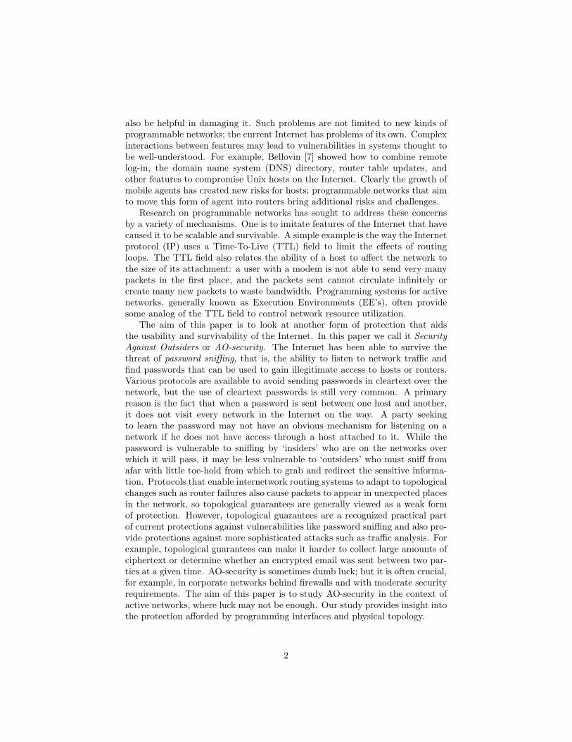
The Internet achieves connectivity by connecting networks through routers.Each network supports the connectivity of a collection of hosts via networkinterfaces. Such an interface can be viewed abstractly as an address pair con-sisting of a network and a location, where a location is a host or router. Figure 1shows an example of this model in which ‘clouds’ represent networks, squaresrepresent routers, and circles represent hosts. To simplify matters we makeno distinction between specific users on hosts and the hosts themselves, so themodel in the figure includes computational agents like Alice and Bob, who haveaddresses on networks n1 and n3 respectively. For Alice to communicate withBob she sends one or more packets to router r1 using network n1. Routers
4
Bob
n4
r3
Alice
Eve
n1 n3r1 r2n2
Claire
Figure 1: Internetwork Example
specialize in knowing how to get packets to where they belong based on a des-tination address provided by the sender; in particular, r1 will probably decideto forward the packets from Alice to Bob to router r3 across network n2. Thisrouter, in turn, will notice that it can get the packets directly to Bob and willcommunicate them to him across network n3. This process causes the com-munication medium consisting of the networks and routers to perform some ofthe functions of a single network. We refer to the collection consisting of thenetworks, routers, and hosts as an internetwork in this paper.
In general, a location l maintains a table that associate a ‘next hop’ witheach destination address. The next hop is an address on a network to which lis attached. The routing table of a host is often simple; for instance, Alice isprobably configured to send packets to (n1, r1) whenever they are for an addressnot on n1. Routers generally maintain more interesting routing tables whichthey develop in a distributed computation involving other routers; the aim ofthis computation is finding paths between each pair of locations on a portionof the internetwork. Several protocols exist to achieve this goal. Two of themost widely-used protocols are RIP [18] and OSPF [19]. In both protocols,each router sends out regular updates of information to aid other routers indetermining how to forward packets. Routers examine the updates that they getfrom each router adjacent to them and modify their routing tables accordingly.In RIP, the updates contain the length and first hop of the shortest known pathto a given destination, while in OSPF the updates contain link informationabout routers around the internetwork.
Many network technologies are subject to ‘sniffing’ of information. For in-stance, an Ethernet LAN broadcasts each message to all of its attached hosts,any one of which may chose to ‘listen’ to messages not addressed to it. For in-stance, when r1 communicates packets from Alice to Bob across n2 for r2, hostslike Claire and routers like r3 that are attached to n2 can collect these packets
5
and read them. This problem can be addressed by encryption, but many or-ganizations have not yet implemented encrypted versions of the protocols. Forinstance, in the RIP and OSPF protocols, the router updates are protected onlyby passwords, which are exchanged in cleartext and hence knowable to anyonewho is on a network that the updates go through. This lack of secrecy threat-ens integrity since anyone who knows the password can issue updates either bymistake or with bad intent. Here is how the RIP RFC on applicability of theprotocol describes the security intention of the passwords [17, page 4]:
The need for authentication in a routing protocol is obvious. It is notusually important to conceal the information in the routing messages, butit is essential to prevent the insertion of bogus routing information intothe routers. So, while the authentication mechanism specified in RIP-2is less than ideal, it does prevent anyone who cannot directly access thenetwork (i.e., someone who cannot sniff the routing packets to determinethe password) from inserting bogus routing information.
This is a description of AO-security for the RIP tables. The OSPF protocolallows passwords on a per-interface basis, and suggests the possibility of usinga password per network. The protection provided by such passwords is char-acterized in the OSPF standard as a safeguard against mistakes [19, pages 205and 206]:
The authentication type is configurable on a per-area basis. Additionalauthentication data is configurable on a per-interface basis. For example,if an area uses a simple password scheme for authentication, a separatepassword may be configured for each network contained in the area. . . .
This guards against routers inadvertently joining the area. They mustfirst be configured with their attached networks’ passwords before theycan participate in the routing domain.
Returning to Figure 1, these properties imply that although Claire may sniffpasswords used between r1 and r2 and therefore may corrupt the routing up-dates with bogus updates, this option will not be available to Eve, who will neversee these passwords on the network to which she is attached. Consider, on theother hand, the internetwork in Figure 2. There is now another router adjacentto Eve, making it possible for Eve to sniff the router update password betweenthe two routers on her network and thus acquire the capability to change rout-ing tables on those routers. Eve may use the information acquired in this wayto corrupt the routers attached to her network. These routers, in turn, maymislead routers to which they send updates, and so on throughout a portion ofthe internetwork. This may allow Eve to cause some or all packets from Alice toBob to go through her network, at least for a while.
Our aim, beginning in the next section, is to develop a language for ex-pressing capabilities so we can talk about AO-security for this internetwork andinternetworks in general. Note first that even for a fixed internetwork the issueis non-trivial. We must characterize what can happen under all of the messagesequences that could be sent by Eve, taking into account all of the ways these
6
r4
n5
r1Alice
Eve
n1 n3r2n2
Claire
r3
n4
Bob
Figure 2: Internetwork Case Study
messages might interact with the updates passing between the routers or themessages between the hosts. Our strategy is to view the internetwork as provid-ing a primitive programming capability. This primitive capability is bolsteredby services offered by the routers and hosts, such as the routing protocol updatesand any other services that may aid communication on the internetwork.
3 A Language-Oriented View of Networking
In this section, we define a language uPLAN inspired by PLAN [14]; veryroughly, it is a small subset of PLAN with the key features needed for ourstudy.
There are other systems for the study of security in distributed and mobilesystems. Specifically, the pi calculus and related formalisms emphasize the con-cept of channel mobility (the capability of creating and communicating channelsdynamically). In contrast, uPLAN deals with a fixed set of communication linksand makes the internetwork topology and the location of computations explicit.In comparison with some other calculi for distributed computation (for exam-ple, the distributed join calculus), our model of distribution is rather concrete,in part because we are trying to model actual active networks, in part becauseof the limitations on mobility. All these calculi have in common, however, theview of some pieces of data as unforgeable and unguessable. This view plays animportant role in the spi calculus, for example, and is crucial in our treatmentof security in this paper.
3.1 Grammar
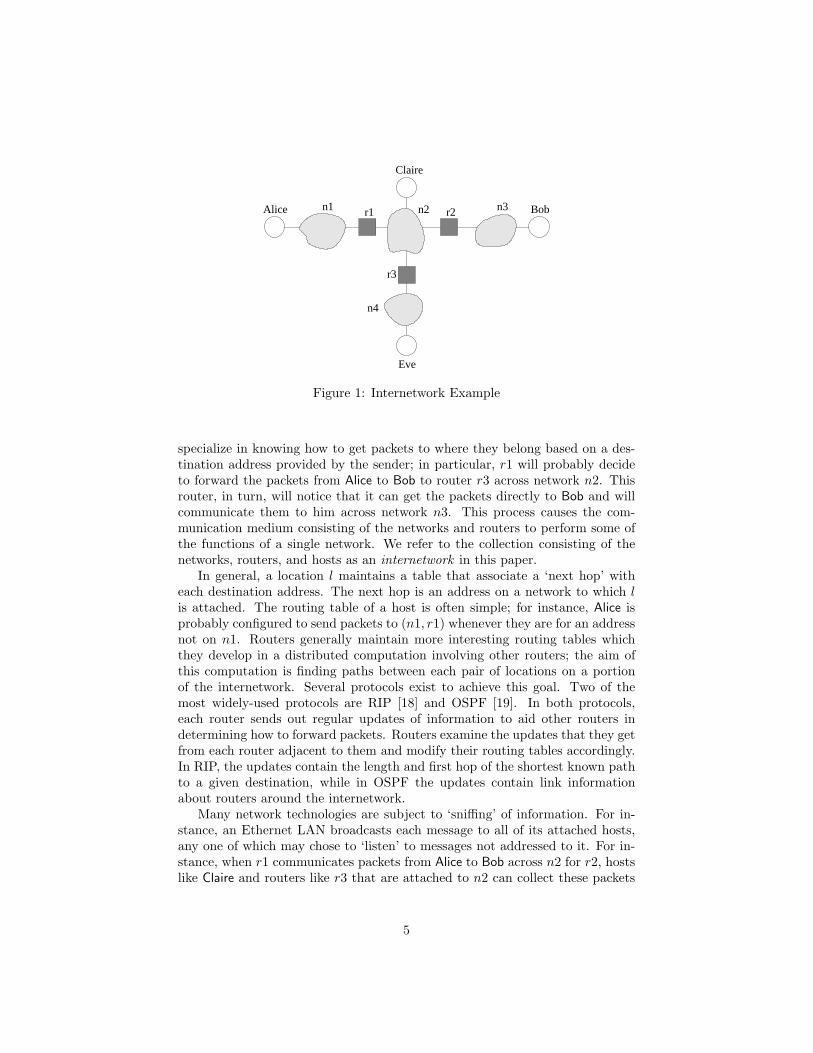
The syntax of uPLAN is given in Table 1. In the programming examples in thepaper, we will use some syntactic sugar, such as allowing functions with multiple
Expressions e ::= x | c | δ |Chunks |x|(e) | |σ|(e)
Remote Evaluation e @ e |Unary Applications x(e) | α(e) | σ(e) |Binary Applications e β e |
Lists and tuples [ ] | [~e] | (e,~e) | #i e |Conditionals e ? e, e |
Sequence e; e |Local Bindings ~d in e
Expression Lists ~e ::= e | e,~e
8
arguments. A simple example based on the internetwork of Figure 1 is a goodplace to begin understanding the concepts in uPLAN. The following programdefines a function for source routing and uses it to route a datum through Aliceto Bob. The program could be evaluated at any location.
fun sourceRoute(l,d) =¬(l=[]) ?(|sourceRoute|(tl(l),d)) @ (hd(l)),deliver(d)
insourceRoute([(n1,Alice),(n3,Bob)], δ)
A program consists of a declaration part and an expression, which is to beevaluated locally. Let us suppose that this program is evaluated by Eve. Thefunction sourceRoute is invoked on a list of two addresses, which happen to bethe interfaces of Alice and Bob, in that order. The function first checks if thelist is empty, and, finding that it is not, makes the following call:
(|sourceRoute|(tl(l),d)) @ (hd(l))
This means the function sourceRoute should be invoked on the list [(n3,Bob)],and this should be done at Alice, the location associated with the address at thehead of the list. The bars surrounding the sourceRoute function are intendedto indicate that this function may not be invoked locally. An expression of theform |f |(x) is called a chunk (short for ‘code hunk’) and represents data at thelocal node. If we write:
val x = |deliver|(3)inx @ (n1,Alice)
The value of x is bound to a pair consisting of a function name deliver and anargument 3. The function associated with deliver depends on the locationwhere it is evaluated.
3.2 Semantics
The semantics of uPLAN is given as a set of transition rules representing com-putational steps applied to a multiset of terms representing network state. Thisform of description can be understood intuitively using a metaphor called a‘chemical abstract machine’ [9] where the state is viewed as a collection of ‘par-ticles’ and computation as a set of ‘reactions’ between these particles. Eachreaction consumes one or more particles and produces one or more. In ourmodel a particle may also be introduced into the mix by an agent (like Alice,Eve, or a router) or removed from it (to represent termination of a computa-tion for instance). Multiset rewriting is well understood in programming lan-guage theory and is easily automated for model checking. For instance, Maude
Local〈S, E, #i e :: C, D〉l −→ Local〈S, E, e :: proji :: C, D〉lLocal〈(v1, . . . , vi, . . . , vn) :: S, E, proji :: C, D〉l −→ Local〈vi :: S, E, C, D〉l
where 1 ≤ i ≤ n
Local〈S, E, x(e) :: C, D〉l −→ Local〈S, E, e :: x :: ap :: C, D〉lLocal〈close(x, x′, e, E′) :: v :: S, E, ap :: C, D〉l −→ Local〈nil, E′′[v/x], e, 〈S, E, C, D〉〉l
where E′′ = E′[close(x, x′, e, E′)/x]Local〈v :: S, E, nil, 〈S′, E′, C′, D′〉〉l −→ Local〈v :: S′, E′, C′, D′〉l
Local〈S, E, α(e) :: C, D〉l −→ Local〈S, E, e :: α :: unary :: C, D〉lLocal〈v :: S, E, α :: unary :: C, D〉l −→ Local〈ConstApply(α, v) :: S, E, C, D〉l
Local〈S, E, σ(e) :: C, D〉l −→ Local〈S, E, e :: serv :: σ :: C, D〉lLocal〈v :: S, E, serv :: σ :: C, D〉l, s, t, z −→ [[σ]](v, k, s, t, z, (S, E, C, D))
Local〈S, E, e β e′ :: C, D〉l −→ Local〈e :: e′ :: β :: binary :: C, D〉lLocal〈v′ :: v :: S, E, β :: binary :: C, D〉l −→ Local〈ConstApply(β, v, v′) :: S, E, C, D〉l
Local〈S, E, e @ e :: C, D〉l −→ Local〈S, E, e :: e′ :: @ :: c, D〉lLocal〈a :: ch :: S, E, @ :: C, D〉l −→ Local〈() :: S, E, C, D〉l, Transit〈a, ch〉l
Local〈S, E, ~d in e :: C, D〉l −→ Local〈nil, E, ~d :: e, 〈S, E, C, D〉〉lLocal〈S, E, d~d :: C, D〉l −→ Local〈S, E, d :: ~d :: C, D〉l
Local〈S, E, val x = e :: C, D〉l −→ Local〈S, E, e :: bind :: x :: C, D〉lLocal〈v :: S, E, bind :: x :: C, D〉l −→ Local〈S, E[v/x], C, D〉lLocal〈S, E, fun x(x′) = e :: C, D〉l −→ Local〈S, E[close(x, x′, e, E)/x], C, D〉l
Local〈S, E, C, D〉l −→
Transit〈(n, l), chunk(x, v, E)〉l −→ Local〈nil, E, x(v), nil〉l
s(l) if l 6∈ Topology(n)s(l) ∪ {δ|δ ∈ v or δ ∈ E} otherwise
s, Σ −→ Local〈nil, ∅, e, nil〉l, s, Σwhere e obeys s(l)and all services σ in e are in Σ
11
(http://maude.csl.sri.com) provides automated support for multiset rewrit-ing and was used to analyze a protocol [22] based on the kind of labeled routingwe discuss below in Section 6.
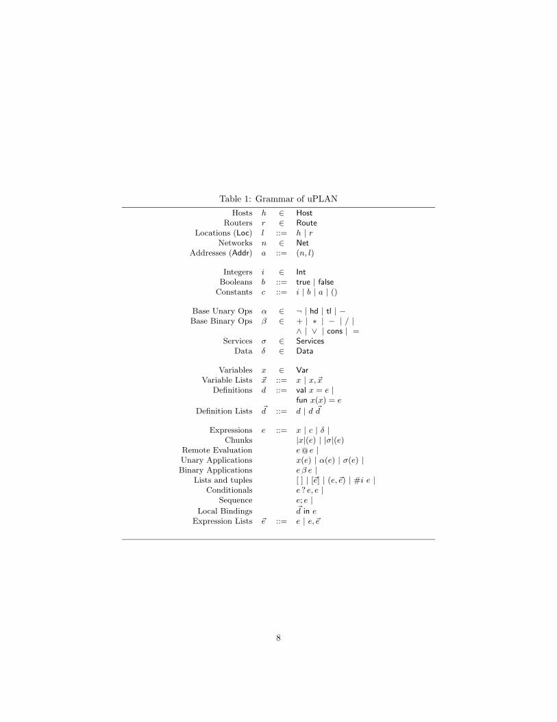
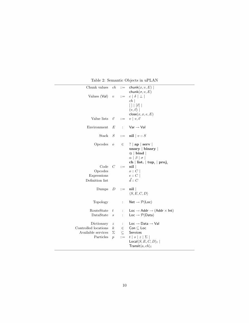
The chemical abstract machine semantics of uPLAN is given in Tables 2and 3. A state of this machine is a multiset of terms we call particles, and eachtransition rule is a rewriting rule on this multiset that replaces some particlesin the multiset with others. A computation Γ is a sequence of states of theabstract machine M1−→M2−→ . . .−→Mk. We write −→∗ for the transitiveclosure of −→. Most of the rules in the table apply to the language constructsof uPLAN, but one rule allows for services σ. The semantics of a service is afunction [[σ]]() of the machine state. The semantics of uPLAN and the servicefunctions allows packets to stop making progress in the network and does nothave any built-in liveness assumptions. In particular, packets will stop makingprogress if no transition rule applies to the current state. The semantics alsoallows for the possibility of packets being dropped from a computation, althoughit does so indirectly by allowing Local〈· · ·〉l particles to be dropped, rather thanTransit〈· · ·〉l particles. In the scenarios that we consider, the possibility thatpackets might be dropped does not cause any secrets to be leaked to outsiders,but that need not always be the case.
We use the notion of ‘controlled’ versus ‘uncontrolled’ locations to model theadversarial behavior of locations. It can be imagined that controlled locationsare those that lie within a single administrative domain, like all machines ina lab that a system administrator controls or all computers operating behinda firewall at a business facility. Our results will be based on the assumptionthat uncontrolled locations may create any particles they wish based on theinformation they have, but controlled locations will create particles accordingto restrictions we place on their behavior. The final rule from Table 3 is calledthe generation rule and represents particles created by hosts and routers. Inmost cases we will state explicitly which particles are produced by the controlledlocations by simply listing them, but in other cases we need to stipulate thatcontrolled locations produce particles using this rule according to a specificprocess they may be running, such as a standard routing protocol. Controlledlocations can be viewed as constituting a system which must react not only toactions of its own participants, but also to arbitrary actions of an environmentof uncontrolled locations.
The internetwork topology is modeled through a map Topology from net-works to sets of locations—each location in the set has an attachment to thenetwork. In a valid topology, hosts are attached to only one network. (Therewould be no difficulty in adding multi-homed hosts to the model.) We modelsecrecy through the notion of a DataState. A DataState, a map from locationsto sets of Data, defines exactly what Data is ‘known’ to a given location. Rout-ing tables are modeled through a RouteState, a map from locations to tables,which are themselves maps from destination addresses to next hop addresseswith integer weights. In a valid RouteState, the next hop for any destinationand any location must be a neighbor, that is, located on a common networkwith the location at which the next hop is computed.
12
To model state on locations, a Dictionary associates with each location atable mapping Data to uPLAN values. We use a special value, ⊥, to representundefined entries in the dictionary. Each entry for which a value hasn’t beenexplicitly defined maps to ⊥. We also define Domainl(z) to be {δ | z(l)(δ) 6= ⊥}.
Locations are constrained to emit only uPLAN programs containing datathat they have ‘learned’. For a datum δ, we say δ ∈ e if δ occurs syntacticallyin the particle e, and we say e obeys s(l) if every δ ∈ e is also a member of s(l).We also extend the relation ∈ to environments and particles and the relationobeys to environments. We say l knows δ in DataState s if δ ∈ s(l).
We consider a valid state M to be a multiset in which there is exactly oneinstance of a DataState, s, one instance of a RouteState, t, one instance of aDictionary, z, and one instance of a set of services Σ. There may be multipleinstances of Transit〈· · ·〉l or Local〈· · ·〉l particles. A Transit〈a, chunk(x, v, E)〉lparticle contains a chunk value and the address where the chunk is to be eval-uated. The particle is routed to the specified address and converted into aLocal〈· · ·〉l particle that evaluates x(v) in the environment E upon arrival at thedestination a. A Local〈S,E,C,D〉l particle contains a program in uPLAN underevaluation at a location. As the nomenclature of the elements of a Local particleimplies, this evaluation happens in an extended version of the SECD abstractmachine [15, 16]. This evaluation may give rise to several new Transit〈· · ·〉l par-ticles before finishing and disappearing. Local〈· · ·〉l particles may also appearspontaneously.
The function ConstApply applies an operator to one or more values andreturns the result of the application. Services are simulated by associating witha service its ‘meaning’, which is a function that takes as arguments the argumentto the service and global internetwork state in the form of current location,DataState, Dictionary, and RouteState, and returns a DataState, Dictionary, andRouteState along with one or more particles. We could constrain this definitionfurther since services will be expected to work only with state at the locationwhere they are invoked. For instance, a service invoked on a router r will notmodify the state on another router r′, but it may cause a message to be sent tor′ which would cause such a change.
4 Some AO-Security Properties
Let us now show how to prove whether AO-security holds in some basic cases.We carry out two analyses, the first assuming that the routers use static routingtables, and the second assuming that they can be dynamically updated. For thefirst of these we can describe a set of particles created by controlled locationsexplicitly, and then analyze the actions the uncontrolled locations may take interms of these. The dynamic update case is more subtle because controlledlocations generate particles based on information they receive from other loca-tions, including possibly uncontrolled locations. The aim of an adversary at anuncontrolled location is to corrupt a controlled router and exploit the spreadof this corruption to other controlled locations using standard routing updates
13
produced by the controlled routers. For each of the static and dynamic caseswe first consider results for a fixed topology, then express a generalization toarbitrary topologies.
4.1 Static Routing Tables
Let us define a basic service deliver to deliver a datum to an intended recipient.We define the value of
[[deliver]](δ, l, s, t, z, (S,E,C,D))
to be Local〈() :: S,E,C,D〉l, s′, t, z where
s′(l′) ={
s(l) ∪ {δ} if l = l′
s(l) otherwise
That is, the deliver service simply causes δ to be added to the data known at thelocation to which it was delivered. For the results in this section let us definethe following particle,
pA = Local〈nil, ∅, |deliver|(δ) @ (n3,Bob),nil〉Alice.
This carries a chunk that causes δ to be added to Bob’s known data.We will first examine properties of the internetwork in Figure 1. We assume
that s is a DataState such that δ 6∈ s(l) unless l = Alice. That is, only Aliceknows δ. We assume that the RouteState t provides shortest routes between alldestinations. That is, a packet moving according to the routing tables reachesits destination after traversing as few networks as the topology allows. In par-ticular, this means the routing tables direct a packet from Alice to Bob alongthe path Alice, r1, r2, Bob. We assume that z is the empty dictionary, and Σincludes only the deliver service.
The following states that if, after Alice initiates the transmission of δ to Bob,there are no particles generated (using the generation rule) by the controlledlocations, then there is no computation in which Eve manages to learn δ. Inthis and subsequent results, Con denotes the controlled locations, and all otherlocations are assumed to be uncontrolled. In this first example all locations areincluded in Con.
Observation 1. Let
Con = {Alice,Bob,Claire,Eve, r1, r2, r3}
and suppose controlled nodes do not generate any particles. If
The proof of the observation is straightforward, noting that the only com-putations possible with these assumptions are initial segments of the one shownin Table 4, where s′ is the same as s except δ ∈ s′(Claire), and s′′ is the sameas s′ except δ ∈ s′(Bob). A very similar observation can also be stated using aninitial assumption that no packets are present, and controlled nodes generateonly the packet pA. Note that t = t′ and z = z′ since there is no interface forchanging the routing tables or dictionary.
The following states the same thing as Observation 1, except this time Eveis an uncontrolled location and thus can initiate transmissions. This extra ca-pability is not enough for Eve to learn the secret being sent from Alice to Bob,even though Eve is able to send packets onto any of the nodes along the pathand have them come back to her using source routing.
Observation 2. Let
Con = {Alice,Bob,Claire, r1, r2, r3}
and suppose controlled nodes do not generate any particles. If
{t, s, z,Σ, pA}−→∗{t′, s′, z′,Σ, p1, . . . , pi},
then δ 6∈ s′(Eve).
However, an outsider located outside of the topological path of a commu-nication can compromise security with the aid of an insider on the path. Theoutsider does not even have to participate in the computation.
Observation 3. Let
Con = {Alice,Bob,Eve, r1, r2, r3}
15
and assume and suppose controlled nodes do not generate any particles. Thenthere is a state s′ such that
{t, s, z,Σ, pA}−→∗{t, s′, z,Σ}and δ ∈ s′(Eve).
These observations can be generalized to an arbitrary topology. Before doingthis, let us be a little more rigorous about the definition of a route.
Definition: A route determined by a RouteState t is a sequence of addressesa1 = (n1, l1), . . . , ap = (np, lp) where (aj+1, i) = t(lj)(ap) and lj 6= lp wheneverj < p. p is the length of the route.
It is possible that there is no route between a pair of locations, but it is uniqueif it exits. The number of addresses on a route is its length. A topology isconnected if it is connected as a graph. In such a topology, routing tables canbe configured so that there is a route between any pair of locations. It will beconvenient to ignore the difference between a location and an address when thelocation is a host, since a host determines a unique address.
The theorem simply says that a datum cannot be learned by a location unlessthe routing tables move it across a network to which the location is attached.Recall that Topology(n) is the set of locations attached to network n.
Theorem 4. Let l1 and l2 be hosts in an arbitrary internetwork and supposethat l2 is attached to network n2. Let
pL = Local〈nil, ∅, |deliver|(δ) @ (n2, l2),nil〉l1and suppose δ 6∈ s(l) for all l 6= l1. Suppose there is a route R between l1 and l2and let
Con = {l | (n, l′) ∈ R and l ∈ Topology(n)}.Suppose controlled nodes do not generate any particles and
{t, s, z,Σ, pL}−→∗{t′, s′, z′,Σ, p1, . . . , pi}.Then δ ∈ s′(l) only if l ∈ Con.
The proof of this result and a selection of other results from the paper canbe found in an appendix.
A few remarks are in order about the limitations of Theorem 4. We haveassumed here that the router tables do not change. In practice, if a network orrouter fails, the routing tables will be altered to find new routes and packetsmay consequently pass along new routes. Eve might even be able to make thishappen by sending so much traffic that a router misses enough transmissionsto conclude that an adjacent router or network is down and modify its routesaccordingly. To model this kind of attack would require an extension of ourframework. We can, however, model the case in which router tables changebecause of updates, and Eve may be able to use these updates.
16
4.2 Dynamic Routing Tables
Routers attempt to be robust with respect to temporary or permanent linkchanges by periodically contacting their neighbors to exchange informationabout routes. These updates can be attacked by an adversary seeking to misleadrouters about the internetwork topology to defeat AO-security. To keep thingsconcrete we focus on using a specific routing protocol for our analysis, althoughanalogous results probably hold for most protocols in current use. In distancevector routing, the routers keep a next hop address for each destination anda distance estimate. The routers periodically provide their current estimatesto their neighbors (locations l1, l2 are neighbors if there is a network n suchthat l1, l2 ∈ Topology(n)) and tables are updated to reflect newly-learned pathestimates. Details of these kinds of protocols can be found in [10, 11]; we willsuppress some of the details to simplify our exposition here.
A RouteState t is said to have shortest routes if there is a route betweenany pair of locations and, for any such pair l1, l2, there is no RouteState t′ thatprovides a shorter path. Distance vector routing finds a shortest path routingtable using the following protocol. Each router r periodically creates particles
Local〈nil, ∅, |routeUpdate|(r, ad, i) @ (n, r′),nil〉rwhere ad is an intended destination, t(r)(ad) = (a, i), and r′ is a neighboron the common network n. These are called advertisements and they indicatedistance estimates to the destination ad. Upon receiving such an advertisement,the router r′ invokes a service routeUpdate which may change the routing tableentry for ad at r′. This service takes as its arguments the router r generatingthe advertisement, the destination ad that the advertisement concerns, and thedistance i where t(r)(ad) = (a, i). Then r′ uses this information to improveits estimate for a route to ad. The salient feature of this protocol is that iteventually calculates shortest path routes and stabilizes. That is, once shortestpath routes are computed, the advertisements do not change routes.
As in the previous subsection, let us begin by analyzing cases for the inter-network in Figure 1. Eve is able to alter the routing tables to suit her purposesin defeating AO-security—she simply sends routing update messages to r1 andr3 that cause all packets meant for Bob to be routed to Eve. (Eve could discardthose packets or obscure her eavesdropping by source-routing them to Bob.)The routers exchange routing updates periodically and may therefore changethe tables back. However, it is possible for Eve to get in her updates at theright time so the packet containing δ is routed to her instead of Bob, making itpossible for her to learn δ. That is, there is (at least) one possible computationwhere Eve can cause routing tables to be corrupted for a long enough periodthat she learns the secret.
Observation 5. Let
Con = {Alice,Bob,Claire, r1, r2, r3}
17
and Σ = {deliver, routeUpdate}. Assume that controlled nodes generate onlyrouter advertisements. Then there exist t′, s′, z′ such that
{t, s, z,Σ, pA}−→∗{t′, s′, z′,Σ}and δ ∈ s′(Eve).
The addition of the routeUpdate service enables an attacker to defeat AO-security for δ.
Let us now consider an alternate service, routeUpdateP, which is used tochange routing tables, but only after a password check. It takes four arguments,with the first three being the same as in routeUpdate, and the fourth being apassword. We assume a mapping from networks to passwords that associatesa password pn to each network n. An invocation of routeUpdateP is valid fora router that receives it from network n if, and only if, the supplied passwordis the password pn assigned to n. As a simplification, we will assume that thispassword is also a member of Data, and is established before computations beginbetween routers attached to a given network.
The analog of Observation 5 will fail when passwords are used to protectrouting updates since Eve will be unable to obtain a password. However, thereis a threat for the internetwork in Figure 2. In this topology, Eve is on anetwork that has two routers attached to it, so updates contain passwords thatcan be sniffed by Eve. Although Eve cannot influence r1 directly, she can doso indirectly, by introducing a spurious entry on r3’s routing table that claimsthat Bob is 0 hops away. The next time r3 sends an update to r1, it will askr1 to change the routing table entry for Bob to r3 if the current entry shows aroute length greater than 1 and this will be true in this internetwork. We againdepend on Eve’s ability to make the spurious updates in time.
Observation 6. Let
Con = {Alice,Bob,Claire, r1, r2, r3}and Σ = {deliver, routeUpdateP}. Assume that controlled nodes generate onlyvalid router advertisements. Then there exist t′, s′, z′ such that
{t, s, z,Σ, pA}−→∗{t′, s′, z′,Σ}and δ ∈ s′(Eve).
Thus even though it is harder for Eve to learn δ in the presence of passwords,she manages to do so. Notice however, that she was only able to do so becauseshe happened to be on a network where advertisements could be seen. If thishad not been true, and if routers followed their protocol, then Eve would nothave been able to learn δ. The following theorem generalizes this property:
Theorem 7. Let l1 and l2 be hosts in an arbitrary internetwork, and assumethat l1 and l2 are attached to networks n1 and n2 respectively. Let
Suppose δ 6∈ s(l) for each l 6= l1, and κn ∈ s(l) if and only if l ∈ Topology(n).Let F be the set of all locations that are only connected to networks containinga unique router. Let Con = (Loc − F) ∪ Topology(n1) ∪ Topology(n2). LetΣ = {deliver, routeUpdateP}. If routers generate only valid advertisements andt provides shortest routes, and
{t, s, z,Σ, pL}−→∗{t′, s′, z′,Σ, p1, . . . , pi},then, for all l ∈ F , δ 6∈ s′(l).
The theorem relies on the assumption that valid advertisements producedby routers do not change routes because shortest routes have been computed.Uncontrolled locations will be unable to create valid advertisements becausethey cannot obtain passwords.
It is non-trivial to formulate a converse for the implication in this theorem.In particular, Eve may have access to router control information but still beunable to learn δ if she is ‘too far away’ from the communication between Aliceand Bob. That is, the topology of the network makes a difference.
5 Bisimilarity and Secrecy
The examples in the previous section illustrate that proofs of properties thatexpress the secrecy (or not) of data in the internetwork are possible. We nowformalize two notions of secrecy for internetworks and prove their equivalence.These results apply to our system without the generation rule. That is, allparticles derive from those originally present. Future work will generalize theseresults so that this restriction is not needed. The formalizations rely on theconcept of AO-security. Here, l is the outsider against whom we want to secureδ.
Definition: A machine state M = {t, s, z,Σ, p1, . . . , pk} provides δ-secrecyagainst l if there is no M ′ such that M ′ = {t′, s′, z′,Σ, p′1, . . . , p
′k′} and M−→∗M ′
and δ ∈ s′(l).
We now define an alternative notion of secrecy that is analogous to the def-inition of secrecy used in the spi calculus [4]. The idea that this definitionexpresses is that a datum remains secret to an external observer if that ob-server’s view of the internetwork is independent of the datum. In particular,changing the datum being transmitted does not change the observer’s view ofthe internetwork. The motivation for such a requirement is that any differencein the behavior of the internetwork could form a covert channel. These ideas goback to treatments of secrecy in terms of noninterference and related conditions.
In order to formalize this idea, we first define an observer’s view of the in-ternetwork in terms of the packets transmitted on any network the observer isattached to. We do this through a labeled transition system, which is derivedfrom the chemical abstract machine defined earlier by partitioning the transi-tion relation defined in Table 3 into two categories. A transition M−→M ′ is
19
observable at l if it involved application of the rule
where t(l′)(a) = ((n, l′′), i) and l ∈ Topology(n). All other transitions are notobservable at l. In the rest of this section, we use M³M ′ for non-observabletransitions, and M
p³M ′ for observable transitions of the form above, where
p = Transit〈a, chunk(x, v, E)〉l′ .We now define the notion of l-bisimulation:
Definition: A relation R between machine states is an l-bisimulation if M1 R
M2 implies that whenever M1³∗ p³³∗M ′
1, then there is some M ′2 such that
M2³∗ p³³∗M ′
2 and M ′1 R M ′
2, and vice versa.
We define l-equivalence ∼l to be the largest l-bisimulation. Thus, M ∼l M ′ ifand only if there is an l-bisimulation R such that M R M ′. The relation ∼l isan equivalence. We have the following
Theorem 8. Let M = {t, s, z,Σ, p1, . . . , pi} and suppose δ 6∈ s(l) and δ′ 6∈ M .If M ∼l M [δ′/δ] then M provides δ-secrecy against l.
That is, if l’s view of the internetwork is the same even when the partiesexchanging secret data use different data, then l does not learn the data. Theconverse is more involved, and requires the following restriction on the kinds ofservices that a program in uPLAN can invoke:
Definition: A service σ is secrecy-friendly if, for every v, l, s, t, S,E,C,D suchthat δ′ 6∈ s, v, S,E,C,D and controlled location l,
This definition expresses the requirement that services are transparent withrespect to data. With this tool in hand, we obtain a converse of the previoustheorem:
Theorem 9. If M = {t, s, z,Σ, p1, . . . , pi} provides δ-secrecy against l andδ′ 6∈ M and all services in Σ are secrecy-friendly, then M ∼l M [δ′/δ]
6 Active Labeled Routing
This section studies AO-security for internetworks in which the routers offerthe ability to set labeled routes. The basic idea of labeled routes is to movea packet along a route based on a label it carries, rather than according to
20
the routing table entries for a final destination. Instead of carrying the entireroute in the packet itself (as in source routing), the packets carry only a label.Before sending any packets that use that label, a source could set up a routeby leaving ‘bread crumbs’ associating labels to intermediate destinations. Thisgives the source more control over the route taken by the packets it sends. Thiscontrol can be exploited to create customized routes that reduce congestion,improve security or reliability, and contribute to other objectives. In scenarioswhere a number of packets are expected to use the same label, this scheme canbe more efficient than source routing and more flexible than default routingusing RIP or OSPF. For example, the PLANet [13] testbed was used to study aprotocol called Flow-Based Adaptive Routing (FBAR) where diagnostic packetswould collect information about congestion, use this to determine custom routesaround congested links, and configure labels to provide alternate routing. Inlabeled routing, as in source routing, the next destination supplied by the labelneed not be an address on an attached network—as it is in a routing table—since default routing (using the routing tables) can be used to get the packetto any destination specified by the label. In the FBAR experiment, routingprovided by RIP was used as a default, with customization provided by labelswhen improvement on the default seemed possible.
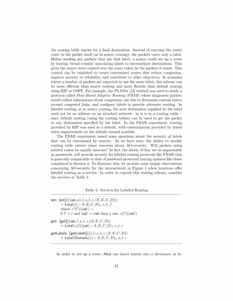
The FBAR experiment raised some questions about the security of labelsthat can be customized by sources. As we have seen, the ability to modifyrouting table entries raises concerns about AO-security. Will packets usinglabeled routes be equally insecure? In fact, the labels, if they are as unguessableas passwords, will provide security for labeled routing protocols like FBAR thatis generally comparable to that of password-protected routing updates like thoseconsidered in Section 4. To illustrate this, let us state some simple observationsconcerning AO-security for the internetwork in Figure 1 when locations offerlabeled routing as a service. In order to express this routing scheme, considerthe services in Table 5.
Table 5: Services for Labeled Routing
set: [[set]]((lab, a), l, s, t, z, (S,E,C,D)))= Local〈() :: S,E,C,D〉l, s, t, z′where z′(l′)(lab′) =if l′ = l and lab′ = lab then a else z(l′)(lab′)
In order to set up a route, Alice can insert entries into a dictionary at lo-
21
cations on the way (starting with Alice herself) associating the label with thenext hop from that location towards the intended final destination, say Bob.This route could be based on any metric that suits Alice. Let us assume herethat it is the shortest route. Thus, a dictionary entry at Alice associates thelabel being used for this route with (n1,r1), an entry at r1 associates the labelwith (n2,r2), and one at r2 associates the label with (n3,Bob). Here’s a uPLANprogram that uses the deliver service defined earlier in conjunction with labeledrouting to route a datum from Alice to Bob:
fun labelRoute(d,l,c,dest) =(c = dest) ?(deliver (d)),(|labelRoute|(d,l,#2(get(l)),dest)) @ (get(l))
inlabelRoute(δ,lab,Alice,Bob)
where δ is the datum to be routed to Bob, and lab is the label that was usedto setup the labeled route from Alice to Bob. Call this program eL. It is similarto source routing, but there is no need for a list of intermediate destinationsin the packet. Once the labeled route has been set up, injecting the particlep = Local〈nil, ∅, eL,nil〉Alice causes δ to be routed to Bob according to the labeledroute.
Consider a scenario in which Eve can get a list of all labels in use at r1.She can then send packets to r1 and try each label in sequence to change thedictionary entries so that the particle containing δ gets routed instead to Eve.This gives Eve a way to learn δ. The following formalizes this property. Here, lets be a DataState such that δ 6∈ s(l) unless l = Alice, and lab 6∈ s(Eve). That is,only Alice knows δ, and Eve does not know the label used to set up the labeledroute. Also, let z be a Dictionary such that z(Alice)(lab) = r1, z(r1)(lab) = r2,z(r2)(lab) = Bob, and all other dictionary entries are undefined.
and assume that the controlled nodes do not generate particles. Then {s, t, z,Σ, p}does not provide δ-secrecy against Eve.
However, if such a facility is not available to Eve, then Eve cannot learn δ.Thus by restricting the service interface appropriately, we can prove guaranteesabout secrecy when labeled routing is in use. The following formalizes thisproperty:
and assume that the controlled nodes do not generate particles. Then {s, t, z,Σ, p}provides δ-secrecy against Eve.
We can generalize this property in two directions. The internetwork underconsideration can be arbitrary, and the labels can point to addresses that areseveral hops away, requiring the use of routing tables which might be corrupted.First, we prove a theorem about an arbitrary network topology and a single hoplabeled route - i.e., a labeled route in which each label points to a location thatis only one hop away.
In the following, eL(δ, lab, l, l′) is the program:
fun labelRoute(d,l,c,dest) =(c = dest) ?(deliver (d)),(|labelRoute|(d,l,#2(get(l)),dest)) @ (get(l))
inlabelRoute(δ,lab,l,l’)
Theorem 12. Let l0 be a host attached to the network n1 in an arbitraryinternetwork. Let a1 = (n1, l1), . . . , ak = (nk, lk) be the sequence such thatli ∈ Topology(ni+1) and z(li)(lab) = (ni+1, li+1), where lab ∈ Data, and z is adictionary in which all other entries are undefined. Let
Suppose δ, lab 6∈ s(l) for all l 6∈ Con and suppose that controlled nodes donot generate new particles. Then {s, t, z,Σ, pL} provides δ-secrecy against alll 6∈ Con.
We now include labeled routes that span multiple hops. Between two lo-cations on the labeled route, the packet would then make use of the routingtables to travel to the next hop. However, now the routeUpdateP service givesan attacker the capability to corrupt routing tables provided the attacker hasaccess to a routing password. As in the last section, κn is the routing passwordfor network n, and will be known to all locations on the network n.
Theorem 13. Let l0 be a host attached to the network n1 in an arbitraryinternetwork. Let a1 = (n1, l1), . . . , ak = (nk, lk) be the sequence such thatz(li)(lab) = (ni+1, li+1), where lab ∈ Data, and z is a dictionary in which allother entries are undefined. Let
Let F be the set of all locations that are only connected to networks containing aunique router. Let Con = (Loc−F) ∪Topology(n1) ∪Topology(n2) and assumecontrolled nodes do not generate any more particles. Suppose δ, lab 6∈ s(l) foreach l 6∈ Con, and κn ∈ s(l) if and only if l ∈ Topology(n). Let t be a shortest-path routing table. Then {s, t, z,Σ, pL} provides δ-secrecy against all l 6∈ Con.
23
7 Conclusions
In this paper we have defined uPLAN as a primitive programming interface foractive networks and used it to demonstrate how to reason about the secrecyof passwords and labels and the integrity of routers. We believe the approachis simple and direct enough to be used routinely for analyzing interfaces whilebeing powerful enough to work for a variety of interesting protocols. We havealso provided a formal treatment of AO-security, which is an important attributeof network protocols. AO-Security plays a significant role in current practice,and it is not always trivial to ensure—as this paper demonstrates in the contextof active networks.
Acknowledgment
We appreciated the help we received on this paper from Roch Guerin, MikeHicks, Trevor Jim, and Jon Moore. This work was supported by DARPA underContract #N66001-96-C-852 and ONR under Contracts N00014-99-1-0403 andN00014-00-1-0641.
A Proofs of various statements
A.1 Theorem 4
Let us examine the sequence of evaluation of pL, that is sent from l1 to l2.Assuming that no other particles are generated, Table 6 shows the evaluationof pL.
In Table 6, sδ is the same as s except all locations on a network on the route
24
R between l1 and l2 have now learned δ. Let
P1L = {p | {t, s, z,Σ, pL}−→∗{t, s′, z,Σ, p}}
andP2
L = {p | {t, s, z,Σ, pL}−→∗{t, s′, z,Σ, p, p′}},and let PL = P1
L ∪P2L. Notice that PL contains all the Local〈. . .〉 particles from
Table 6 along with Transit〈. . .〉 particles of the following form:
Transit〈(n2, l2), chunk(deliver, δ, ∅)〉lwhere l is a location on the route between l1 and l2. This is true because theparticle pL gets turned into a Transit〈〉 particle of the above form with l beingl1, and is intended to reach the address (n2, l2).
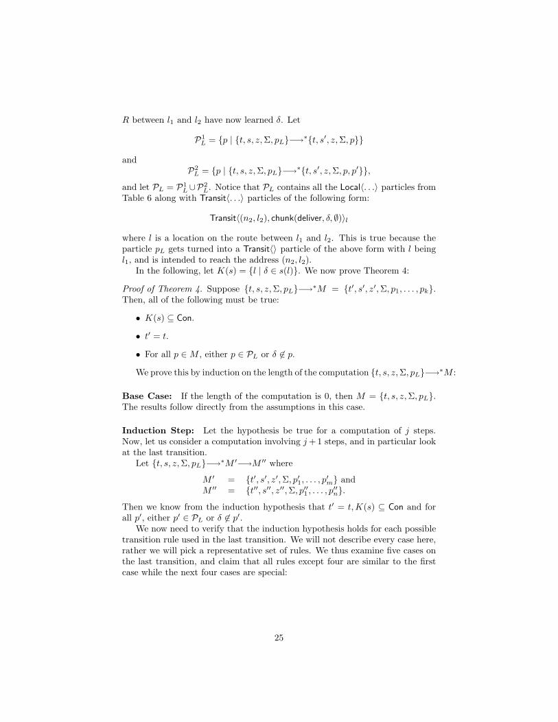
In the following, let K(s) = {l | δ ∈ s(l)}. We now prove Theorem 4:
Proof of Theorem 4. Suppose {t, s, z,Σ, pL}−→∗M = {t′, s′, z′,Σ, p1, . . . , pk}.Then, all of the following must be true:
• K(s) ⊆ Con.
• t′ = t.
• For all p ∈ M , either p ∈ PL or δ 6∈ p.
We prove this by induction on the length of the computation {t, s, z,Σ, pL}−→∗M :
Base Case: If the length of the computation is 0, then M = {t, s, z,Σ, pL}.The results follow directly from the assumptions in this case.
Induction Step: Let the hypothesis be true for a computation of j steps.Now, let us consider a computation involving j +1 steps, and in particular lookat the last transition.
Let {t, s, z,Σ, pL}−→∗M ′−→M ′′ where
M ′ = {t′, s′, z′,Σ, p′1, . . . , p′m} and
M ′′ = {t′′, s′′, z′′,Σ, p′′1 , . . . , p′′n}.Then we know from the induction hypothesis that t′ = t,K(s) ⊆ Con and forall p′, either p′ ∈ PL or δ 6∈ p′.
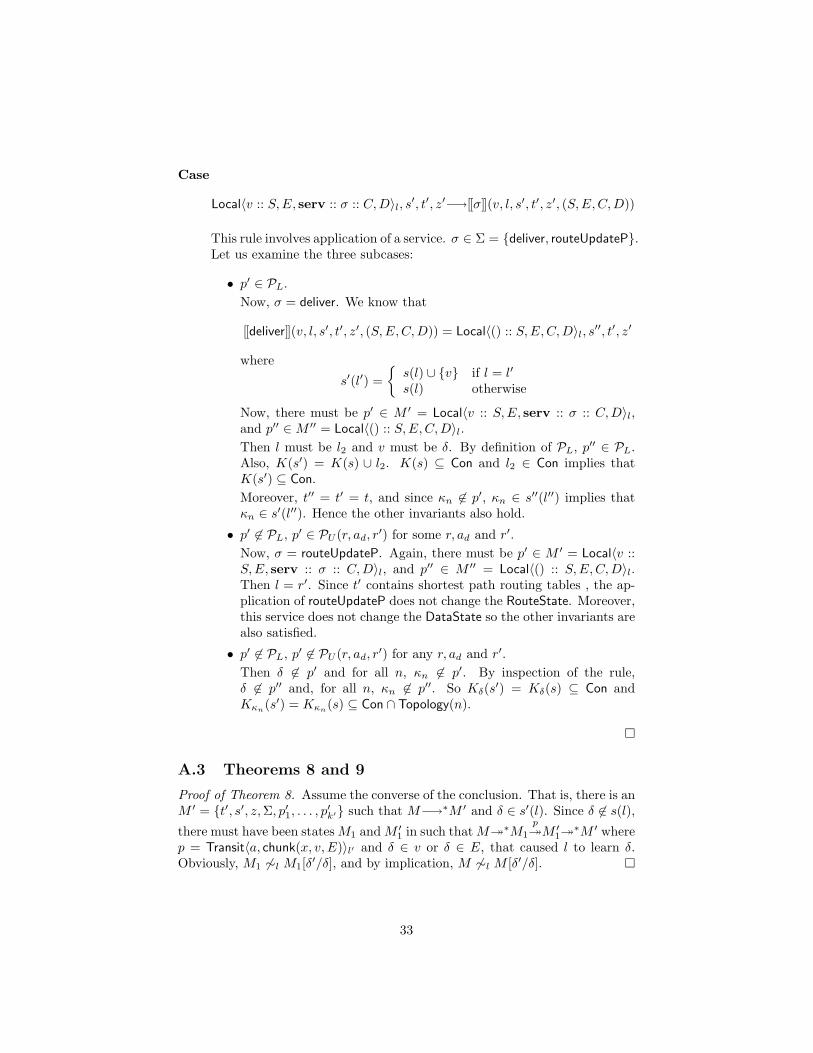
We now need to verify that the induction hypothesis holds for each possibletransition rule used in the last transition. We will not describe every case here,rather we will pick a representative set of rules. We thus examine five cases onthe last transition, and claim that all rules except four are similar to the firstcase while the next four cases are special:
Thus, there is some p′ ∈ M ′ and some p′′ ∈ M ′′ such that p′ = Local〈v ::S,E, ch :: σ :: C,D〉k and p′′ = Local〈chunk(σ, v, E) :: S,E,C,D〉k. Nowthere are two subcases:
• p′ ∈ PL.From the definition of P , {t, s, z,Σ, pL}−→∗{t, s′, z,Σ, p′}. Since{t, s′, z,Σ, p′}−→{t, s′, z,Σ, p′′}, we must have p′′ ∈ PL.
• p′ 6∈ PL.From the induction hypothesis then δ 6∈ p′, and by an inspection ofthe rule, δ 6∈ p′′.
In both subcases, this rule does not change either the DataState or theRouteState, thus t′′ = t′ = t and s′′ = s′ therefore K(s) ⊆ Con.
s′(l′′) if l′′ 6∈ Topology(n)s′(l′′) ∪ {δ|δ ∈ v or δ ∈ E} otherwise
This rule changes the DataState. Now, there must be some p′ ∈ M ′ andsome p′′ ∈ M ′′ such that p′ = Transit〈a, ch〉l and p′′ = Transit〈a, ch〉l′ .Notice that the rule does not change the RouteState, hence t′′ = t′ = t.Again, there are two subcases:
• p′ ∈ PL.Then l is a location on the route from l1 to l2. By the definitionof a route, l′ must also be a location on the route, and from theassumptions in the statement of the Theorem, if l′′ ∈ Topology(n)then l′′ ∈ Con.Now, p′ must be Transit〈(n2, l2), chunk(deliver, δ, ∅)〉l, so δ ∈ p′. Ifl′′ ∈ K(s′′), then δ ∈ s′′(l′′), so either δ ∈ s′(l′′) or l′′ ∈ Topology(n)and in both cases l′′ ∈ Con, by the induction hypothesis for the formerand from the preceding paragraph for the latter.Also by definition of PL, p′′ ∈ PL.
• p′ 6∈ PL.Then δ 6∈ p′, so δ ∈ s′′(l′′) only if δ ∈ s′(l′′) only if l′′ ∈ Con. Also,by inspection of the rule, δ 6∈ p′′.
26
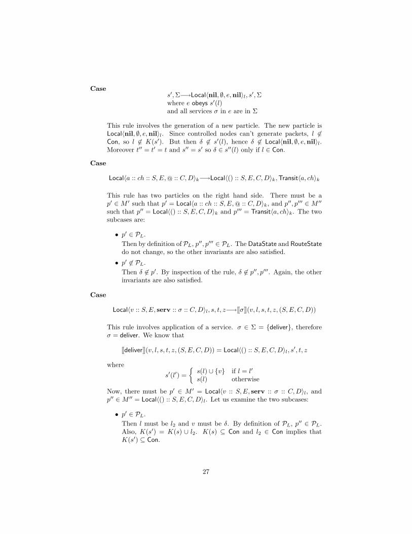
Cases′,Σ−→Local〈nil, ∅, e,nil〉l, s′,Σwhere e obeys s′(l)and all services σ in e are in Σ
This rule involves the generation of a new particle. The new particle isLocal〈nil, ∅, e,nil〉l. Since controlled nodes can’t generate packets, l 6∈Con, so l 6∈ K(s′). But then δ 6∈ s′(l), hence δ 6∈ Local〈nil, ∅, e,nil〉l.Moreover t′′ = t′ = t and s′′ = s′ so δ ∈ s′′(l) only if l ∈ Con.
Now, there must be p′ ∈ M ′ = Local〈v :: S,E, serv :: σ :: C,D〉l, andp′′ ∈ M ′′ = Local〈() :: S,E,C,D〉l. Let us examine the two subcases:
• p′ ∈ PL.Then l must be l2 and v must be δ. By definition of PL, p′′ ∈ PL.Also, K(s′) = K(s) ∪ l2. K(s) ⊆ Con and l2 ∈ Con implies thatK(s′) ⊆ Con.
27
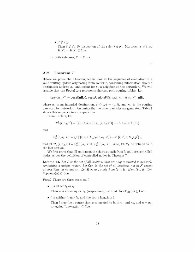
• p′ 6∈ PL.Then δ 6∈ p′. By inspection of the rule, δ 6∈ p′′. Moreover, v 6= δ, soK(s′) = K(s) ⊆ Con.
In both subcases, t′′ = t′ = t.
A.2 Theorem 7
Before we prove the Theorem, let us look at the sequence of evaluation of avalid routing update originating from router r, containing information about adestination address ad, and meant for r′, a neighbor on the network n. We willassume that the RouteState represents shortest path routing tables. Let
pU (r, ad, r′) = Local〈nil, ∅, |routeUpdateP|(r, ad, i, κn) @ (n, r′),nil〉r
where ad is an intended destination, t(r)(ad) = (a, i), and κn is the routingpassword for network n. Assuming that no other particles are generated, Table 7shows this sequence in a computation.
the last section.We first prove that all routers on the shortest path from l1 to l2 are controlled
nodes as per the definition of controlled nodes in Theorem 7:
Lemma 14. Let F be the set of all locations that are only connected to networkscontaining a unique router. Let Con be the set of all locations not in F exceptall locations on n1 and n2. Let R be any route from l1 to l2. If (n, l) ∈ R, thenTopology(n) ⊆ Con.
Proof. There are three cases on l:
• l is either l1 or l2.
Then n is either n1 or n2 (respectively), so that Topology(n) ⊆ Con.
• l is neither l1 nor l2, and the route length is 3.
Then l must be a router that is connected to both n1 and n2, and n = n1,so again, Topology(n) ⊆ Con.
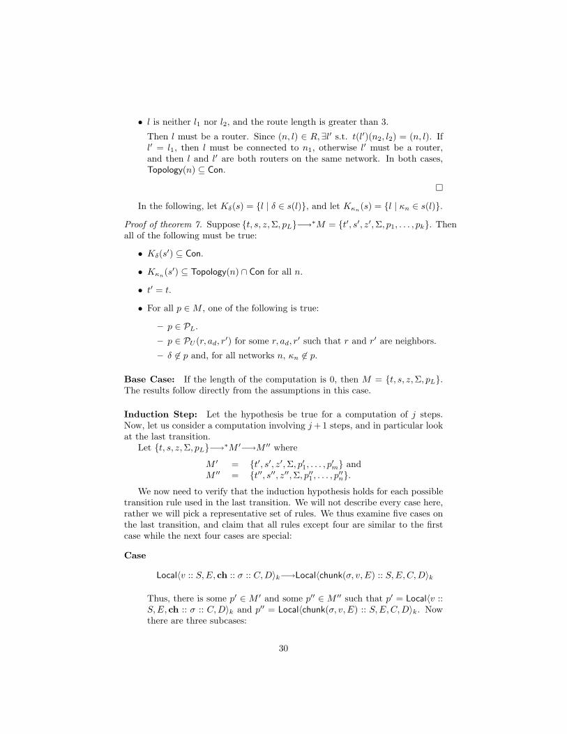
• l is neither l1 nor l2, and the route length is greater than 3.
Then l must be a router. Since (n, l) ∈ R,∃l′ s.t. t(l′)(n2, l2) = (n, l). Ifl′ = l1, then l must be connected to n1, otherwise l′ must be a router,and then l and l′ are both routers on the same network. In both cases,Topology(n) ⊆ Con.
In the following, let Kδ(s) = {l | δ ∈ s(l)}, and let Kκn(s) = {l | κn ∈ s(l)}.
Proof of theorem 7. Suppose {t, s, z,Σ, pL}−→∗M = {t′, s′, z′,Σ, p1, . . . , pk}. Thenall of the following must be true:
• Kδ(s′) ⊆ Con.
• Kκn(s′) ⊆ Topology(n) ∩ Con for all n.
• t′ = t.
• For all p ∈ M , one of the following is true:
– p ∈ PL.
– p ∈ PU (r, ad, r′) for some r, ad, r
′ such that r and r′ are neighbors.
– δ 6∈ p and, for all networks n, κn 6∈ p.
Base Case: If the length of the computation is 0, then M = {t, s, z,Σ, pL}.The results follow directly from the assumptions in this case.
Induction Step: Let the hypothesis be true for a computation of j steps.Now, let us consider a computation involving j +1 steps, and in particular lookat the last transition.
Let {t, s, z,Σ, pL}−→∗M ′−→M ′′ where
M ′ = {t′, s′, z′,Σ, p′1, . . . , p′m} and
M ′′ = {t′′, s′′, z′′,Σ, p′′1 , . . . , p′′n}.We now need to verify that the induction hypothesis holds for each possible
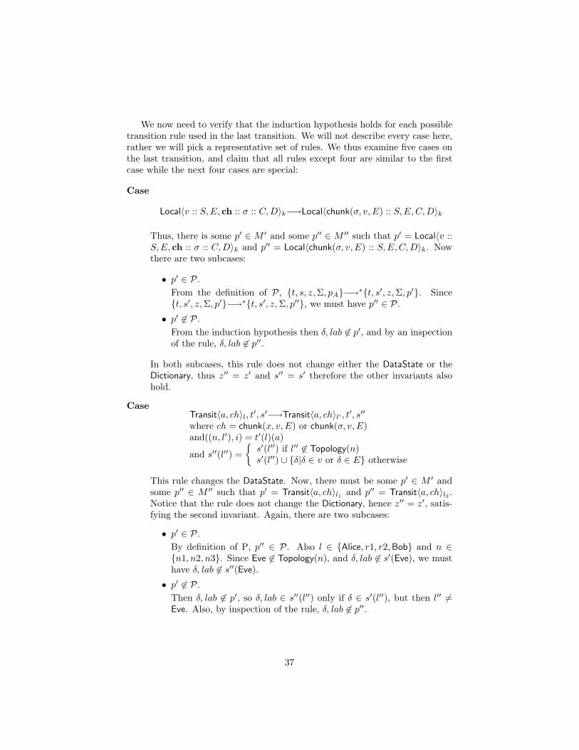
transition rule used in the last transition. We will not describe every case here,rather we will pick a representative set of rules. We thus examine five cases onthe last transition, and claim that all rules except four are similar to the firstcase while the next four cases are special:
Thus, there is some p′ ∈ M ′ and some p′′ ∈ M ′′ such that p′ = Local〈v ::S,E, ch :: σ :: C,D〉k and p′′ = Local〈chunk(σ, v, E) :: S,E,C,D〉k. Nowthere are three subcases:
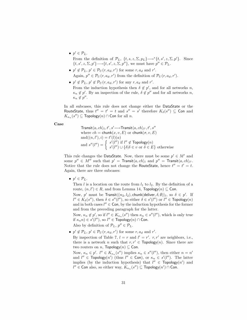
30
• p′ ∈ PL.From the definition of PL, {t, s, z,Σ, pL}−→∗{t, s′, z,Σ, p′}. Since{t, s′, z,Σ, p′}−→{t, s′, z,Σ, p′′}, we must have p′′ ∈ PL.
• p′ 6∈ PL, p′ ∈ PU (r, ad, r′) for some r, ad and r′.
Again, p′′ ∈ PU (r, ad, r′) from the definition of PU (r, ad, r
′).
• p′ 6∈ PL, p′ 6∈ PU (r, ad, r′) for any r, ad and r′.
From the induction hypothesis then δ 6∈ p′, and for all networks n,κn 6∈ p′. By an inspection of the rule, δ 6∈ p′′ and for all networks n,κn 6∈ p′′.
In all subcases, this rule does not change either the DataState or theRouteState, thus t′′ = t′ = t and s′′ = s′ therefore Kδ(s′′) ⊆ Con andKκn
s′(l′′) if l′′ 6∈ Topology(n)s′(l′′) ∪ {δ|δ ∈ v or δ ∈ E} otherwise
This rule changes the DataState. Now, there must be some p′ ∈ M ′ andsome p′′ ∈ M ′′ such that p′ = Transit〈a, ch〉l and p′′ = Transit〈a, ch〉l′ .Notice that the rule does not change the RouteState, hence t′′ = t′ = t.Again, there are three subcases:
• p′ ∈ PL.Then l is a location on the route from l1 to l2. By the definition of aroute, (n, l′) ∈ R, and from Lemma 14, Topology(n) ⊆ Con.Now, p′ must be Transit〈(n2, l2), chunk(deliver, δ, ∅)〉l, so δ ∈ p′. Ifl′′ ∈ Kδ(s′′), then δ ∈ s′′(l′′), so either δ ∈ s′(l′′) or l′′ ∈ Topology(n)and in both cases l′′ ∈ Con, by the induction hypothesis for the formerand from the preceding paragraph for the latter.Now, κn 6∈ p′, so if l′′ ∈ Kκn
(s′′) then κn ∈ s′′(l′′), which is only trueif κnn) ∈ s′(l′′), so l′′ ∈ Topology(n) ∩ Con.Also by definition of PL, p′′ ∈ PL.
• p′ 6∈ PL, p′ ∈ PU (r, ad, r′) for some r, ad and r′.
By inspection of Table 7, l = r and l′ = r′. r, r′ are neighbors, i.e.,there is a network n such that r, r′ ∈ Topology(n). Since there aretwo routers on n, Topology(n) ⊆ Con.Now, κn ∈ p′. l′′ ∈ Kκn
(s′′) implies κn ∈ s′′(l′′), then either n = n′
and l′′ ∈ Topology(n′) (thus l′′ ∈ Con), or κn ∈ s′(l′′). The latterimplies (by the induction hypothesis) that l′′ ∈ Topology(n′) andl′′ ∈ Con also, so either way, Kκn
(s′′) ⊆ Topology(n′) ∩ Con.
31
In this case, δ 6∈ p′, so l′′ ∈ Kδ(s′′) implies that δ ∈ s′′(l′′) which isonly true if δ ∈ s′(l′′), so l′′ ∈ Con.Also, by definition of PU (r, ad, r
′), p′′ ∈ PU (r, ad, r′).
• p′ 6∈ PL, p′ 6∈ PU (r, ad, r′) for any r, ad and r′.
Then δ 6∈ p′, so δ ∈ s′′(l′′) only if δ ∈ s′(l′′) only if l′′ ∈ Con. Also, byinspection of the rule, δ 6∈ p′′. The same argument holds for all κn.
Cases′,Σ−→Local〈nil, ∅, e,nil〉l, s′,Σwhere e obeys s′(l)and all services σ in e are in Σ
This rule involves the generation of a new particle. The new particlep = Local〈nil, ∅, e,nil〉l. There are two subcases:
• l ∈ Con. Then the new particle can only be a valid routing up-date, and then p ∈ PU (r, ad, r
′) for some r, ad, r′ such that r, r′ are
neighbors.
• l 6∈ Con. Then l 6∈ Kδ(s′) and l 6∈ Kκn(s′) for all n. But then
This rule has two particles on the right hand side. There must be a p′ ∈ M ′
such that p′ = Local〈a :: ch :: S,E,@ :: C,D〉k, and p′′, p′′′ ∈ M ′′ suchthat p′′ = Local〈() :: S,E,C,D〉k and p′′′ = Transit〈a, ch〉k. The threesubcases are:
• p′ ∈ PL.Then by definition of PL, p′′, p′′′ ∈ PL. The DataState and RouteStatedo not change, so the other invariants are also satisfied.
• p′ 6∈ PL, p′ ∈ PU (r, ad, r′) for some r, ad and r′.
Again, by definition, p′′ ∈ PU (r, ad, r′). Again, other invariants are
also satisfied.
• p′ 6∈ PL, p′ 6∈ PU (r, ad, r′) for any r, ad and r′.
Then δ 6∈ p′ and for all n, κn 6∈ p′. By inspection of the rule,δ 6∈ p′′, p′′′ and for all n, κn 6∈ p′′, p′′′. Again, the other invariants arealso satisfied.
Now, there must be p′ ∈ M ′ = Local〈v :: S,E, serv :: σ :: C,D〉l,and p′′ ∈ M ′′ = Local〈() :: S,E,C,D〉l.Then l must be l2 and v must be δ. By definition of PL, p′′ ∈ PL.Also, K(s′) = K(s) ∪ l2. K(s) ⊆ Con and l2 ∈ Con implies thatK(s′) ⊆ Con.Moreover, t′′ = t′ = t, and since κn 6∈ p′, κn ∈ s′′(l′′) implies thatκn ∈ s′(l′′). Hence the other invariants also hold.
• p′ 6∈ PL, p′ ∈ PU (r, ad, r′) for some r, ad and r′.
Now, σ = routeUpdateP. Again, there must be p′ ∈ M ′ = Local〈v ::S,E, serv :: σ :: C,D〉l, and p′′ ∈ M ′′ = Local〈() :: S,E,C,D〉l.Then l = r′. Since t′ contains shortest path routing tables , the ap-plication of routeUpdateP does not change the RouteState. Moreover,this service does not change the DataState so the other invariants arealso satisfied.
• p′ 6∈ PL, p′ 6∈ PU (r, ad, r′) for any r, ad and r′.
Then δ 6∈ p′ and for all n, κn 6∈ p′. By inspection of the rule,δ 6∈ p′′ and, for all n, κn 6∈ p′′. So Kδ(s′) = Kδ(s) ⊆ Con andKκn
(s′) = Kκn(s) ⊆ Con ∩ Topology(n).
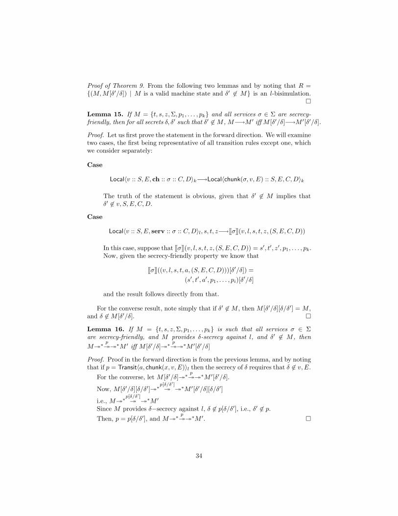
A.3 Theorems 8 and 9
Proof of Theorem 8. Assume the converse of the conclusion. That is, there is anM ′ = {t′, s′, z,Σ, p′1, . . . , p
′k′} such that M−→∗M ′ and δ ∈ s′(l). Since δ 6∈ s(l),
there must have been states M1 and M ′1 in such that M³∗M1
p³M ′
1³∗M ′ wherep = Transit〈a, chunk(x, v, E)〉l′ and δ ∈ v or δ ∈ E, that caused l to learn δ.Obviously, M1 6∼l M1[δ′/δ], and by implication, M 6∼l M [δ′/δ].
33
Proof of Theorem 9. From the following two lemmas and by noting that R ={(M,M [δ′/δ]) | M is a valid machine state and δ′ 6∈ M} is an l-bisimulation.
Lemma 15. If M = {t, s, z,Σ, p1, . . . , pk} and all services σ ∈ Σ are secrecy-friendly, then for all secrets δ, δ′ such that δ′ 6∈ M , M−→M ′ iff M [δ′/δ]−→M ′[δ′/δ].
Proof. Let us first prove the statement in the forward direction. We will examinetwo cases, the first being representative of all transition rules except one, whichwe consider separately:
For the converse result, note simply that if δ′ 6∈ M , then M [δ′/δ][δ/δ′] = M ,and δ 6∈ M [δ′/δ].
Lemma 16. If M = {t, s, z,Σ, p1, . . . , pk} is such that all services σ ∈ Σare secrecy-friendly, and M provides δ-secrecy against l, and δ′ 6∈ M , thenM³∗ p
³³∗M ′ iff M [δ′/δ]³∗ p³³∗M ′[δ′/δ]
Proof. Proof in the forward direction is from the previous lemma, and by notingthat if p = Transit〈a, chunk(x, v, E)〉l then the secrecy of δ requires that δ 6∈ v,E.
For the converse, let M [δ′/δ]³∗ p³³∗M ′[δ′/δ].
Now, M [δ′/δ][δ/δ′]³∗p[δ/δ′]³ ³∗M ′[δ′/δ][δ/δ′]
i.e., M³∗p[δ/δ′]³ ³∗M ′
Since M provides δ−secrecy against l, δ 6∈ p[δ/δ′], i.e., δ′ 6∈ p.Then, p = p[δ/δ′], and M³∗ p
³³∗M ′.
34
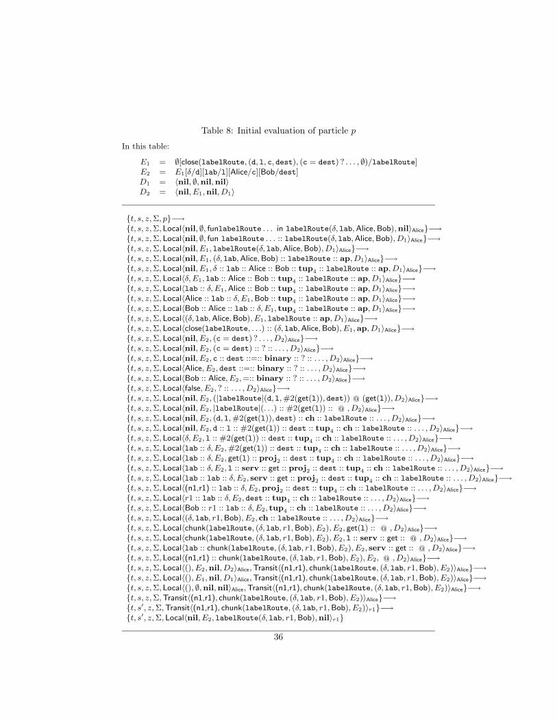
A.4 Observation 11
In order to prove this observation, we first define the set P to be the set ofall particles that appear in the computation of a labeled routing particle, p =Local〈nil, ∅, eL,nil〉Alice, in the following way: let
P1 = {p′ | {t, s, z,Σ, p}−→∗{t, s′, z,Σ, p′}}and
P2 = {p′ | {t, s, z,Σ, p}−→∗{t, s′, z,Σ, p′, p′′}},and let P = P1 ∪ P2.
We can provide a detailed description of an exact computation starting fromthe machine state {t, s, z,Σ, p}, following the example of the proofs of Theo-rems 4 and 7. It turns out however that the computation here would spanseveral pages. We therefore provide in Table 8 only the first few steps in theevaluation of particle p. Notice that the last machine state in the table looks al-most exactly like the fourth one, with three differences: Alice has been replacedwith r1, the environment in the only Local〈. . .〉 particle has some extra entrieswhich will not get used, and the DataState has been augmented so that all lo-cations on n1 now know the secrets δ and lab. The rest of this computationwill repeat the pattern shown in the table, once at r1 and then at r2, and thenwill end at Bob.
We now prove the Observation.
Proof of Observation 11. Suppose {t, s, z,Σ, p}−→∗M = {t′, s′, z′,Σ, p1, . . . , pk}.Then all of the following must be true:
• δ, lab 6∈ s′(Eve).
• z′(l)(lab) = z(l)(lab) for all l ∈ {Alice, r1, r2,Bob}, and z′(l)(δ′) 6= lab, δfor all l ∈ Loc and all δ′ ∈ Data.
• For all p ∈ M , one of the following must hold:
– p ∈ P.
– δ, lab 6∈ p.
We prove this by induction on the length of the computation {t, s, z,Σ, p}−→∗M .
Base Case: If the length of the computation is 0, then M = {t, s, z,Σ, p}.The results follow directly from the assumptions in this case.
Induction Step: Let the hypothesis be true for a computation of j steps.Now, let us consider a computation involving j +1 steps, and in particular lookat the last transition.
We now need to verify that the induction hypothesis holds for each possibletransition rule used in the last transition. We will not describe every case here,rather we will pick a representative set of rules. We thus examine five cases onthe last transition, and claim that all rules except four are similar to the firstcase while the next four cases are special:
Thus, there is some p′ ∈ M ′ and some p′′ ∈ M ′′ such that p′ = Local〈v ::S,E, ch :: σ :: C,D〉k and p′′ = Local〈chunk(σ, v, E) :: S,E,C,D〉k. Nowthere are two subcases:
• p′ ∈ P.From the definition of P, {t, s, z,Σ, pA}−→∗{t, s′, z,Σ, p′}. Since{t, s′, z,Σ, p′}−→∗{t, s′, z,Σ, p′′}, we must have p′′ ∈ P.
• p′ 6∈ P.From the induction hypothesis then δ, lab 6∈ p′, and by an inspectionof the rule, δ, lab 6∈ p′′.
In both subcases, this rule does not change either the DataState or theDictionary, thus z′′ = z′ and s′′ = s′ therefore the other invariants alsohold.
s′(l′′) if l′′ 6∈ Topology(n)s′(l′′) ∪ {δ|δ ∈ v or δ ∈ E} otherwise
This rule changes the DataState. Now, there must be some p′ ∈ M ′ andsome p′′ ∈ M ′′ such that p′ = Transit〈a, ch〉l1 and p′′ = Transit〈a, ch〉l2 .Notice that the rule does not change the Dictionary, hence z′′ = z′, satis-fying the second invariant. Again, there are two subcases:
• p′ ∈ P.By definition of P, p′′ ∈ P. Also l ∈ {Alice, r1, r2,Bob} and n ∈{n1, n2, n3}. Since Eve 6∈ Topology(n), and δ, lab 6∈ s′(Eve), we musthave δ, lab 6∈ s′′(Eve).
• p′ 6∈ P.Then δ, lab 6∈ p′, so δ, lab ∈ s′′(l′′) only if δ ∈ s′(l′′), but then l′′ 6=Eve. Also, by inspection of the rule, δ, lab 6∈ p′′.
37
Cases′,Σ−→Local〈nil, ∅, e,nil〉l, s′,Σwhere e obeys s′(l)and all services σ in e are in Σ
This rule involves the generation of a new particle. The new particle isLocal〈nil, ∅, e,nil〉l. Since controlled nodes can’t generate packets, l =Eve, so δ, lab 6∈ s′(l). But δ, lab 6∈ Local〈nil, ∅, e,nil〉l. Moreover z′′ = z′
This rule involves application of a service. σ ∈ Σ = {set, get, deliver}.[[σ]](v, l, s′, t′, z′, (S,E,C,D)) = p′′, s′′, t′′, z′′. Let us examine the two sub-cases:
• p′ ∈ P.Then σ is either get or deliver.
– If σ = get, z′′ = z′ and s′′ = s′.– If σ = deliver, we must have l = Bob. Now, z′′ = z′, and δ, lab ∈
s′′(l′′) only if δ, lab ∈ s′(l′′) or l′′ = Bob, thus δ, lab 6∈ s′′(Eve).
Also, by definition of P, p′′ ∈ P.
• p′ 6∈ P.Then δ, lab 6∈ p′. Let us examine three subcases on σ:
– If σ = get, z′′ = z′ and s′′ = s′. Since z′(l)(δ′) 6= δ, lab for alll ∈ Loc and all δ′ ∈ Data, so δ, lab 6∈ p′′.
38
– If σ = set, s′′ = s′. Since δ, lab 6∈ p′, z′′(l)(lab) = z′(l)(lab) forall l, and z′′(l)(δ′) 6= δ, lab for all l ∈ Loc and all δ′ ∈ Data. Byinspection of the definition of set, δ, lab 6∈ p′′.
– If σ = deliver, z′′ = z′. Moreover, δ, lab 6∈ p′ and δ, lab 6∈ s′(Eve)imply that δ, lab 6∈ s′′(Eve). Again, by inspection of the definitionof deliver, δ, lab 6∈ p′′.
A.5 Theorem 12
Again, we define the set of particles PL to be the set of particles arising duringthe computation of the particle pL in the following way: let
P1L = {p′ | {t, s, z,Σ, pL}−→∗{t, s′, z,Σ, p′}}
andP2
L = {p′ | {t, s, z,Σ, pL}−→∗{t, s′, z,Σ, p′, p′′}},and let PL = P1
L ∪ P2L.
The evaluation of pL will be similar to the evaluation in the last proof,hence we don’t provide a detailed table here. The computation will involvea series of Local〈. . .〉 and Transit〈. . .〉 particles, with the former evaluating oneach successive location li in the labeled route, and the latter being one-hopmovements from one location in the route to the next.
We now prove the theorem. In the following, let Kδ(s) = {l | δ ∈ s(l)}, andlet Klab(s) = {l | lab ∈ s(l)}.Proof of Theorem 12. Suppose {t, s, z,Σ, pL}−→∗M = {t′, s′, z′,Σ, p1, . . . , pk}.Then all of the following must be true:
• Kδ(s′) ⊆ Con.
• Klab(s′) ⊆ Con.
• z′(li)(lab) = z(li)(lab) and z′(l)(δ′) 6= lab, δ for all l ∈ Loc and all δ′ ∈Data.
• For all p ∈ M , one of the following must hold:
– p ∈ PL.
– δ, lab 6∈ p.
We prove this by induction on the length of the computation {t, s, z,Σ, pL}−→∗M .
Base Case: If the length of the computation is 0, then M = {t, s, z,Σ, pL}.The results follow directly from the assumptions in this case.
39
Induction Step: Let the hypothesis be true for a computation of j steps.Now, let us consider a computation involving j +1 steps, and in particular lookat the last transition.
Let {t, s, z,Σ, pL}−→∗M ′−→M ′′ where
M ′ = {t′, s′, z′,Σ, p′1, . . . , p′m} and
M ′′ = {t′′, s′′, z′′,Σ, p′′1 , . . . , p′′n}.We now need to verify that the induction hypothesis holds for each possible
transition rule used in the last transition. We will not describe every case here,rather we will pick a representative set of rules. We thus examine five cases onthe last transition, and claim that all rules except four are similar to the firstcase while the next four cases are special:
Thus, there is some p′ ∈ M ′ and some p′′ ∈ M ′′ such that p′ = Local〈v ::S,E, ch :: σ :: C,D〉k and p′′ = Local〈chunk(σ, v, E) :: S,E,C,D〉k. Nowthere are two subcases:
• p′ ∈ PL.From the definition of PL, {t, s, z,Σ, pL}−→∗{t, s′, z,Σ, p′}. Since{t, s′, z,Σ, p′}−→∗{t, s′, z,Σ, p′′}, we must have p′′ ∈ PL.
• p′ 6∈ PL.From the induction hypothesis then δ, lab 6∈ p′, and by an inspectionof the rule, δ, lab 6∈ p′′.
In both subcases, this rule does not change either the DataState or theDictionary, thus z′′ = z′ and s′′ = s′ therefore the other invariants alsohold.
s′(l′′) if l′′ 6∈ Topology(n)s′(l′′) ∪ {δ | δ ∈ v or δ ∈ E} otherwise
This rule changes the DataState. Now, there must be some p′ ∈ M ′ andsome p′′ ∈ M ′′ such that p′ = Transit〈a, ch〉l′ and p′′ = Transit〈a, ch〉l′′ .Notice that the rule does not change the Dictionary, hence z′′ = z′, satis-fying the third invariant. Again, there are two subcases:
• p′ ∈ PL.By definition of PL, l = li for some i, and a = (ni+1, li+1, 0). Sinceli ∈ Topology(ni+1) and t′ is a shortest path routing table, t′(l)(a) =
40
a. Thus n = ni+1 and l′ = li+1, thus p′′ ∈ PL. Also Topology(n) ⊆Con. Consider some l′′ 6∈ Con. Since l′′ 6∈ Topology(n), and δ, lab 6∈s′(l′′), we must have δ, lab 6∈ s′′(l′′), so that Kδ(s′′),Klab(s′′) ⊆ Con.
• p′ 6∈ PL.Then δ, lab 6∈ p′, so δ, lab ∈ s′′(l′′) only if δ ∈ s′(l′′), but then l′′ ∈Con, so that Kδ(s′′),Klab(s′′) ⊆ Con. Also, by inspection of the rule,δ, lab 6∈ p′′.
Cases′,Σ−→Local〈nil, ∅, e,nil〉l, s′,Σwhere e obeys s′(l)and all services σ in e are in Σ
This rule involves the generation of a new particle. The new particle isLocal〈nil, ∅, e,nil〉l. Since controlled nodes can’t generate packets, l 6∈Con, so δ, lab 6∈ s′(l). But then δ, lab 6∈ Local〈nil, ∅, e,nil〉l. Moreoverz′′ = z′ and s′′ = s′ so the other invariants also hold.
This rule involves application of a service. σ ∈ Σ = {set, get, deliver}.[[σ]](v, l, s′, t′, z′, (S,E,C,D)) = p′′, s′′, t′′, z′′. Let us examine the two sub-cases:
• p′ ∈ PL.Then σ is either get or deliver.
– If σ = get, z′′ = z′ and s′′ = s′.
41
– If σ = deliver, we must have l = lk, so l ∈ Con. Now, z′′ = z′,and δ, lab ∈ s′′(l′′) only if δ, lab ∈ s′(l′′) or l′′ = lk, and thusKδ(s′′),Klab(s′′) ⊆ Con.
Also, by definition of PL, p′′ ∈ PL.
• p′ 6∈ PL.Then δ, lab 6∈ p′. Let us examine three subcases on σ:
– If σ = get, z′′ = z′ and s′′ = s′. Since z′(l)(δ′) 6= δ, lab for alll ∈ Loc and all δ′ ∈ Data, so δ, lab 6∈ p′′.
– If σ = set, s′′ = s′. Since δ, lab 6∈ p′, z′′(l)(lab) = z′(l)(lab) forall l, and z′′(l)(δ′) 6= δ, lab for all l ∈ Loc and all δ′ ∈ Data. Byinspection of the definition of set, δ, lab 6∈ p′′.
– If σ = deliver, z′′ = z′. Moreover, δ, lab 6∈ p′ and Kδ(s′),Klab(s′) ⊆Con imply that Kδ(s′′),Klab(s′′) ⊆ Con. Again, by inspection ofthe definition of deliver, δ, lab 6∈ p′′.
42
References
[1] Martın Abadi. Secrecy by typing in security protocols. In Theoreti-cal Aspects of Computer Software, volume 1281 of LNCS, pages 611–638.Springer, September 1997.
[2] Martın Abadi. Secrecy by typing in security protocols. Journal of the ACM,46(5):749–786, September 1999.
[3] Martın Abadi. Security protocols and specifications. In Foundations ofSoftware Science and Computation Structures: Second International Con-ference, FOSSACS ’99, pages 1–13. Springer-Verlag, March 1999.
[4] Martın Abadi and Andrew D. Gordon. A calculus for cryptographic proto-cols: The spi calculus. Information and Computation, 148(1):1–70, January1999.
[5] D. Scott Alexander, William A. Arbaugh, Angelos D. Keromyts, andJonathan M. Smith. A secure active network environment architecture:Realization in SwitchWare. IEEE Network Magazine, 1998. To appear inthe special issue on Active and Controllable Networks.
[6] D. Scott Alexander, Marianne Shaw, Scott M. Nettles, and Jonathan M.Smith. Active Bridging. In Proceedings, 1997 SIGCOMM Conference.ACM, 1997.
[7] Steven M. Bellovin. Using the domain name system for system break-ins.In Proceedings of the Fifth USENIX UNIX Security Symposium, June 1995.
[8] G. Berry and G. Boudol. The chemical abstract machine. In Proceedingsof the 17th Annual Symposium of Programming Languages, pages 81–94,1990.
[9] Gerard Berry and Gerard Boudol. The chemical abstract machine. Theo-retical Computer Science, 96:217–248, 1992.
[10] Dimitri P. Bertsekas and Robert Gallager. Data Networks. Prentice Hall,1991.
[11] Karthikeyan Bhargavan, Davor Obradovic, and Carl A. Gunter. Formalverification of standards for distance vector routing protocols, February2000.
[12] Michael Hicks and Angelos D. Keromytis. A secure PLAN. In StefanCovaci, editor, Proceedings of the First International Working Conferenceon Active Networks, volume 1653 of Lecture Notes in Computer Science,pages 307–314. Springer-Verlag, June 1999.
43
[13] Michael Hicks, Jonathan T. Moore, D. Scott Alexander, Carl A. Gunter,and Scott Nettles. PLANet: An active internetwork. In Proceedings of theEighteenth IEEE Computer and Communication Society Infocom Confer-ence, pages 1124–1133. IEEE Communication Society Press, March 1999.
[14] Mike Hicks, Pankaj Kakkar, Jonathan T. Moore, Carl A. Gunter, and ScottNettles. PLAN: A packet language for active networks. In Proceedings ofthe Third ACM SIGPLAN International Conference on Functional Pro-gramming Languages, pages 86–93. ACM, 1998.
[15] P. Landin. The mechanical evaluation of expressions. Comput. J., 6:308–320, 1964.
[16] P. Landin. An abstract machine for designers of computing languages. InIFIP Congress, pages 438–439. North-Holland, 1965.
[17] G. Malkin. RIP Version 2 Applicability Statement. IETF RFC 1722,November 1994.
[18] G. Malkin. RIP Version 2 Carrying Additional Information. IETF RFC1723, November 1994.
[19] J. Moy. OSPF version 2. RFC 1583, IETF, March 1994.
[20] Jonathan M. Smith, Kenneth L. Calvert, Sandra L. Murphy, Hilarie K.Orman, and Larry L. Peterson. Activating networks: A progress report.IEEE Computer, 32(4):32–41, April 1999.
[21] David L. Tennenhouse, Jonathan M. Smith, W. David Sincoskie, David J.Wetherall, and Gary J. Minden. A survey of active network research. IEEECommunications Magazine, 35(1):80–86, January 1997.
[22] Bow-Yaw Wang, Jose Meseguer, and Carl A. Gunter. Specification andformal verification of a PLAN algorithm in Maude. In Tenh Lai, editor,Proceedings of the 2000 ICDCS Workshop on Distributed System Validationand Verification, pages E:49–E:56. IEEE Computer Society, April 2000.
[23] David J. Wetherall, John Guttag, and David L. Tennenhouse. ANTS: AToolkit for Building and Dynamically Deploying Network Protocols. InIEEE OPENARCH, April 1998.