Rec. ITU-R SM.1055-0 1

RECOMMENDATION ITU-R SM.1055-0*

THE USE OF SPREAD SPECTRUM TECHNIQUES

(1994) Rec. ITU-R SM.1055

The ITU Radiocommunication Assembly,

considering

a) that spread spectrum systems can offer improved sharing factors in certain conditions in achieving

telecommunications objectives;

b) that spread spectrum systems include frequency-hopping, direct sequence, and mixed frequency-hopping-direct

sequence systems;

c) that spread spectrum systems can offer operational advantages such as increased resistance to interference and

improved performance under multipath conditions;

d) that the mutual interference between spread spectrum signals, and between spread spectrum signals and more

traditional narrow-band signals requires further study;

e) that spread spectrum systems operate differently from more traditional narrow-band communications,

recommends

1. that the descriptions of spread spectrum technologies and signal-to-noise calculations contained in Annex 1, be

recognized when describing direct sequence (DS), frequency-hopping (FH), and combination frequency-hopping/direct-

sequence (FH/DS) modulations;

2. that the signal-to-interference ratios, the minimum required propagation losses, and other performance

degradation measures between potential interferers as described in Annex 2 should be used when studying the effect of

individual frequency-hopping and direct-sequence spread spectrum signals on several common signals on a one-to-one

basis, including AM (A3E), FM (F3E), wideband FDM/FM (F8E), and television;

3. that the procedure described in Annex 3 be used when calculating the effect of direct-sequence and frequency-

hopping systems on digital receivers, AM voice receivers, and FM voice receivers.

Note 1 – Additional studies should focus on the effects of multiple spread spectrum interferers in a crowded environment.

ANNEX 1

Spread spectrum techniques

1. Introduction

This Annex describes broadband “spread spectrum” techniques and the interference rejection capabilities of

these systems.

A spread spectrum (SS) system can be defined as one in which the average energy of the transmitted signal is

spread over a bandwidth which is much wider than the information bandwidth (the bandwidth of the transmitted signal is

wider than the information bandwidth by at least a factor of two for double sideband AM and typically a factor of four or

greater for narrow-band FM, and 100 to 1 for a linear SS system). These systems essentially trade the wider transmission

bandwidth for a lower power spectral density and increased rejection to interfering signals operating in the same

frequency band. They, therefore, have the potential of sharing the spectrum with conventional narrow-band systems

_______________

* Radiocommunication Study Group 1 made editorial amendments to this Recommendation in the year 2018 in accordance with

Resolution ITU-R 1.

2 Rec. ITU-R SM.1055-0

because of the potentially low power that is transmitted in the narrow-band receiver passband. In addition, high levels of

interference will be rejected by SS receiving systems. These systems should therefore be examined to identify how

efficiently they use the spectrum.

Two distinct types of bandwidth expansion SS techniques need to be discussed. These are the techniques that

provide either linear or non-linear interference signal rejection. The classical FM approach typifies non-linear techniques

because there is only an increase in the output S/N ratio (dB) when the input S/N is greater than the first or noise capture

ratio. This means that the input S/N must be typically greater than 10 dB in order to obtain a linear enhancement against

noise. In contrast to the FM type of system, the SS systems described in this Annex are linear so that the improvement

remains constant even if the input wanted-to-unwanted signal ratio is negative. The output wanted signal-to-interference

signal ratio (S/I)out is increased over the input wanted signal-to-interference ratio (S/I)in and is defined as the processing

gain (PG) of the system. This PG might typically be 100 to 1, or larger. PG is defined by the following:

10 log PG (S/I )out – (S/I )in (1)

A system with a PG of 100 (and no loss due to non-ideal signal processing) and a minimum output S/I of 10 dB

requires that the input S/I is, at least;

(S/I )in 10 dB – 10 log 100 –10 dB

A linear SS system that can operate with an input (S/I) of –10 dB is extremely desirable since with an unwanted

signal 10 dB higher than the wanted signal, the system can still be effectively used. For conventional systems with an

input (S/I) of –10 dB, the wanted signal would be suppressed or “captured” and no information would be transferred.

A second major feature of commonly used SS techniques is that the resulting transmitted signal is a wideband

low-power-density signal which resembles noise. Therefore, the transmitted signal is not readily detected by a

conventional receiver. Recovery of the baseband information from the wideband transmitted signal can be accomplished

only through correlation or matched filter (MF) signal processing. Because of this property, the unintended listener does

not detect the baseband information, and because of the low power density, it may not cause any significant interference

effects to other users of the spectrum. SS inherently provides a degree of message privacy to non-SS systems as well as

other SS systems using different codes and no special signal processing. The coding also provides a selective addressing

capability. Multiple users using different codes (code division multiple access – CDMA) can simultaneously transmit in

the same frequency band with a minimum amount of cross interference (codes that are used should have a low cross-

correlation function).

A third advantage of SS techniques over conventional modulation techniques is increased transmission

reliability in the presence of selective fading and multipath effects. This advantage can be significant for typically

encountered fading transmission mediums, e.g. in tropospheric scatter systems. Increased resistance to multipath is a

direct consequence of spreading the transmitted bandwidth. As a first approximation, improvement is directly

proportional to the ratio of transmitted bandwidth to information bandwidth. Receivers built to detect SS signals typically

generate, prior to their final demodulation, a cross-correlation function between a replica of the transmitted signal and the

signal received from the antenna. The correlation function of the wanted signal is always chosen to be as “good” as

possible, i.e. maximum output at the centre and the signal falling to near zero in a time period equal to the reciprocal of

the transmitted signal bandwidth and staying at near zero at all other times. Multipath degrades link performance when it

combines with the direct signal in such a manner as to degrade the correlation function of the detected signal by reducing

its peak value. The introduction of false trailing peaks into the correlation function due to simple multipath is typically

not a problem. The receiver will detect and process the first peak of adequate amplitude, either the direct signal if it is

strong enough or the first reflected signal of adequate amplitude if the direct signal is interfered with. In the latter case,

timing becomes synchronized to the multipath return and it is processed in lieu of the direct signal. Consequently, for

multipath to be destructive, it must occur with a differential delay less than the duration

Rec. ITU-R SM.1055-0 3

of the peak of the correlation function, with a phase that causes destructive interference (cancellation rather than

enhancement) and with an amplitude adequate to prevent the peak from exceeding detection thresholds. As the

transmitted bandwidth is increased, the duration of the correlation function peak is proportionally decreased, and the

multipath differential path delay that can affect performance is also proportionally decreased.

2. Spread spectrum signal types

Definitions for various types of spread spectrum techniques/signal structure are as follows:

– Direct sequence (DS) spread spectrum: a signal structuring technique utilizing a digital code spreading sequence

having a chip rate 1/Tsin much higher than the information signal bit rate 1/Ts. Each information bit of the digital

signal is transmitted as a pseudo-random sequence of chips, which produces a broad noise-like spectrum with a

bandwidth (distance between first nulls) of 2 Bsin 2/Tsin

. The receiver correlates the RF input signal with a local

copy of the spreading sequence to recover the narrow-band data information at a rate 1/Ts.

– Frequency-hopping (FH) spread spectrum: a signal structuring technique employing automatic switching of the

transmitted frequency. Selection of the frequency to be transmitted is typically made in a pseudo-random manner

from a set of frequencies covering a band wider than the information bandwidth. The intended receiver frequency-

hops in synchronization with the transmitter in order to retrieve the desired information.

– Hybrid spread spectrum (FH/DS): a combination of frequency-hopping spread spectrum and direct-sequence spread

spectrum.

– Chip rate: the rate at which the successive bits of the spreading sequence is applied to the signal information.

Two other types of spread spectrum modulation exist. The first uses pulsed frequency modulation or “chirped

modulation” in which a carrier is swept over a band of frequencies. Radar systems, in particular, may use a sweep rate

that is a linear function of time. The second spread spectrum type employs a non-sinusoidal carrier to provide additional

processing gain. The following discussion does not include chirped or non-sinusoidal spread spectrum types.

3. Signal-to-noise (S/N) performance of DS and FH systems

The (S/N) performance of a linear DS spread spectrum system in the presence of Gaussian noise applies to

receiver system noise and external noise with Gaussian characteristics. For this condition, DS performance is given by:

PG (S/N )out

(S/N )in 2 Bsin

Ts (2)

where:

PG : processing gain of the system

(S/N)out : output signal-to-noise ratio (correlator output)

(S/N)in : input signal-to-noise ratio (RF input)

2 Bsin : bandwidth of RF input signal power density spectrum at first nulls

Ts : time duration of input signal information.

The processing gain (equation (2)) is considered the most important parameter of an SS system.

The peak of the code rate signal autocorrelation function at u 0 will have a duration of the order 1/Bsin Tsin

.

The ratio of the duration of the signal information (Ts) to the main peak response is thus given by Ts /Tsin. Thus the large

Bsin Ts case affords a “pulse compression” effect whereby the signal energy in a relatively long pulse (duration of Ts) is

“compressed” into a high level short pulse (duration of Tsin ). The result is a high detection probability at the intended

receiver with no loss in time resolution.

4 Rec. ITU-R SM.1055-0

The same results can be obtained in the time domain by taking the inverse Fourier transform of the respective

functions and using equivalent time operations.

The FH system basically consists of a narrow-band filter matched to the information bandwidth pseudo-

randomly shifting in frequency over the SS bandwidth. The noise out of the system is therefore governed by the

bandwidth of the narrow filter. When an analysis is made of noise or an unwanted interfering signal which occupies the

full hopping bandwidth, a decrease in the output unwanted signal power is obtained which is equal to the ratio of the

bandwidths. The PG for this case is, therefore, equal to:

PG BFH

Bs (3)

where:

BFH : FH bandwidth

Bs : wanted information bandwidth.

If the FH system utilized the same RF bandwidth as the RF bandwidth in the DS system to the first nulls and

transmits the same information rate, the BFH and Bs in equation (3) are respectively equal to 2 Bsin and 1/Ts in

equation (2) so that the processing gain of both systems is the same, neglecting second order effects. It should be noted

that this is only for the case of a noise or an unwanted signal spread over the wide bandwidth and not for a narrow-band

signal. The sensitivity of the FH system does not contain the PG improvement of the DS system and is simply

proportional to the noise temperature of the system and the information bandwidth.

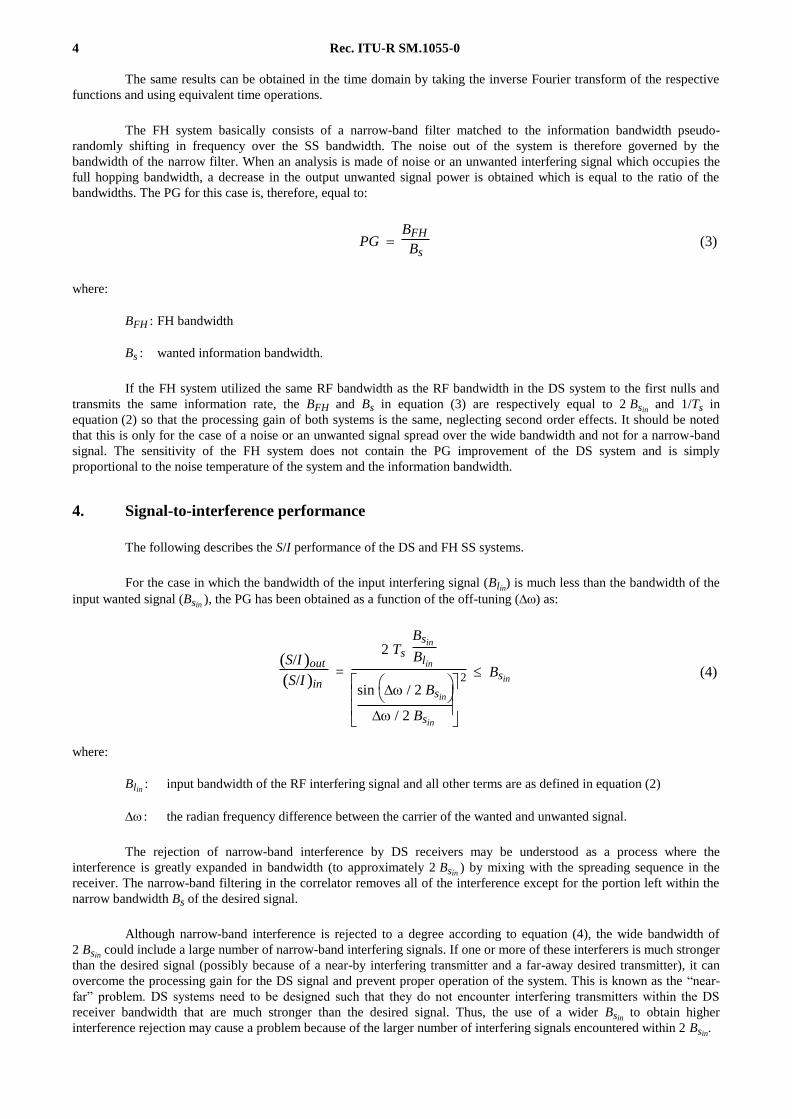
4. Signal-to-interference performance

The following describes the S/I performance of the DS and FH SS systems.

For the case in which the bandwidth of the input interfering signal (Blin) is much less than the bandwidth of the

input wanted signal (Bsin ), the PG has been obtained as a function of the off-tuning () as:

( )S/I out

( )S/I in =

2 Ts Bsin

Blin

sin

/ 2 Bsin

/ 2 Bsin

2 Bsin (4)

where:

Blin : input bandwidth of the RF interfering signal and all other terms are as defined in equation (2)

: the radian frequency difference between the carrier of the wanted and unwanted signal.

The rejection of narrow-band interference by DS receivers may be understood as a process where the

interference is greatly expanded in bandwidth (to approximately 2 Bsin ) by mixing with the spreading sequence in the

receiver. The narrow-band filtering in the correlator removes all of the interference except for the portion left within the

narrow bandwidth Bs of the desired signal.

Although narrow-band interference is rejected to a degree according to equation (4), the wide bandwidth of

2 Bsin could include a large number of narrow-band interfering signals. If one or more of these interferers is much stronger

than the desired signal (possibly because of a near-by interfering transmitter and a far-away desired transmitter), it can

overcome the processing gain for the DS signal and prevent proper operation of the system. This is known as the “near-

far” problem. DS systems need to be designed such that they do not encounter interfering transmitters within the DS

receiver bandwidth that are much stronger than the desired signal. Thus, the use of a wider Bsin to obtain higher

interference rejection may cause a problem because of the larger number of interfering signals encountered within 2 Bsin.

Rec. ITU-R SM.1055-0 5

When the bandwidth of the interference is greater than the wanted signal, the PG has been obtained as:

(S/I )out

(S/I )in =

2

Blin

Bsin Ts Bsin

sin

/ 2 Blin

/ 2 Blin

2 (5)

This clearly shows that the gain is proportional to the bandwidth filtering ratio and the time bandwidth product

as would have been expected. From the point of view of the output power ratios, the wideband SS system overcomes

interference to the same degree that it overcomes noise.

In the FH SS system, the frequency hopper re-inserts the correct carrier frequency for the wanted signal and

mixes it to the IF centre frequency. Any interfering signal, entering at a fixed frequency relative to the centre frequency of

the FH SS system, is converted after the FH to a signal of reduced amplitude and random off-tuned frequency due to the

FH mixer and IF filter action.

The interfering signal is then filtered so that effectively only those signals that fall within the same frequency

channel as the desired signal are transferred through the system as interference. Since there are n possible frequency

channels, this happens on an average only 1/nth of the time.

The interference at the input to the detector is, therefore, similar to a Poisson process. The degradation in the

receiver output depends upon the signal processing structure. Since this structure heavily affects the degradation analysis,

no simple generalization can be given for required input (S/I) ratios. However, the determination of what degradation

results depends upon the structure of the receiver and the input (S/I) ratio.

FH systems do not necessarily suffer from the “near-far” problems that affect DS systems. Since a strong

narrow-band interferer will affect only a small number of hops, it will cause only a small number of errors (which can be

handled through forward error-correction techniques). A smart FH system may even note which hops contain interfering

signals and choose alternative frequencies.

If the interference consists of a uniform wideband amplitude modulated (AM) signal that equals the FH

bandwidth, the hopper output signal consists approximately of a constant amplitude signal with a random frequency offset

term. For this case, the degradation analysis consists of essentially analysing an unwanted FM signal, reduced in power by

the ratio of the bandwidths (equation (3)), against whatever subsequent type of signal processing structure is being

employed by the frequency hopper. If the detection structure consists of a frequency modulated (FM) or phase modulated

(PM) structure, the PG will be similar to that obtained against noise except for low (S/I) ratios where an FM capture

effect will be introduced.

If the interference consists of a wideband FM signal that equals in bandwidth the FH bandwidth, the hopper

output signal consists of a somewhat random amplitude signal with a random frequency offset. The effect of this signal

would be very similar to the noise interference case so that the PG is given by equation (3) and the required (S/I) ratio is

the same as required for the Gaussian noise case.

5. Spectrum efficiency

Since SS systems use more bandwidth to transmit a given amount of information than a conventional narrow-

band system, the question of how efficiently the spectrum is being used should be considered. Spectrum use efficiency is

generally a product of bandwidth, geometric space and time. The problem which therefore requires examination from the

viewpoint of spectrum efficiency is how many narrow-band and SS systems can transmit simultaneously in the same

frequency band and same geographical area, particularly for a high density of systems. This problem is under study in

many arenas, with system designers trying to efficiently exploit the special characteristics of SS systems.

6 Rec. ITU-R SM.1055-0

The use of SS systems in bands reserved for SS systems may prove to be a good solution for high-density

mobile communications. In this case, the wide bandwidth of SS systems prevents the deep Rayleigh fading which occurs

with conventional narrow-band systems, allowing lower power transmitters to provide reliable operation. Field tests

of FH mobile radio equipment in the frequency band of about 800 MHz with Reed-Solomon coding and soft decision

decoding have been carried out in Japan. The result shows a considerable reduction in bit errors, making use of the

frequency-diversity effect. A laboratory experiment performed using a fading simulator showed a 17 dB decrease in

required power for a BER of 10–3. Similar results were obtained in a field test in urban areas, and in addition, the

irreducible errors which are often encountered on digital transmission in mobile radio communications did not occur.

Thus, it has been experimentally verified that the FH technique can tolerate significant fading in urban areas.

The spectrum efficiency issue should be addressed in detail in future studies on SS systems.

6. Summary

SS systems have been defined and descriptions of the DS, FH, and FH/DS techniques have been given. The PG

has been shown for various interference cases to be proportional to the spread bandwidth divided by the information

bandwidth. For many SS systems the PG can be a large positive number which allows the operation of the systems when

the input interference is much greater than the wanted signal. This is the case in which the wanted output information

would be lost for a typical narrow-band system. The large signal bandwidths required for many SS applications result in

low power spectral density signals. Small numbers of these low power spectral density signals potentially cause negligible

performance degradation to systems using conventional modulation techniques in the same frequency band, assuming that

the total power density received from SS systems remains sufficiently below the desired conventional signal levels. In

addition, SS systems can provide improved resistance to deep fading, resulting in system design advantages and improved

spectrum efficiency.

ANNEX 2

Examples of band sharing by employing spread spectrum techniques

1. Introduction

A characteristic of a spread spectrum (SS) system is that the emitted signal bandwidth is typically much greater

than the bandwidth of the message being transmitted. The large bandwidths and associated low power spectral densities

used by these systems potentially make them less likely to interfere with conventional systems operating in the same

environment, unless the number of active SS systems is large enough to raise the apparent background noise level.

Two sets of examples are given to show the potential sharing between SS and other modulation techniques.

2. Factors to consider in band sharing

The ability of two or more systems to share a band with an acceptable level of electromagnetic compatibility

involves a number of factors specific to the systems being considered. In general, however, successful systems band

sharing may necessitate a trade off between three conditions at the receivers of the systems.

Condition 1 – The wanted signal power delivered to the receivers must, with reasonable probability, exceed an

acceptable threshold value to assure high detection probability of the shortest time duration signal element the receiver is

capable of recognizing.

Rec. ITU-R SM.1055-0 7

The factors influencing satisfaction of this condition are the conventional considerations that apply in any link

calculation. Transmitter power should be the minimum needed as determined both by receiver sensitivity and expected

variation in propagation path loss. Antenna characteristics should be consistent with coverage requirements. Receiver

characteristics are the result of compromise at the designing stage to achieve sensitivity and dynamic-range balance and

to account for transmitted signal tolerances and relative station motions.

Condition 2 – In the presence of interference, the signal-to-interference S/I ratio must exceed an acceptable

threshold with reasonable probability. Typical factors influencing satisfaction of this condition are:

– interference power minimization by such techniques as transmitter power limitation, antenna nulling, low-duty-

factor, and low spectral density;

– orthogonal signal structure designs that produce different exploitable characteristics where the S/I ratio can be

enhanced by signal processing;

– receiver discrimination factors which take account of what existing receivers do rather than what is ideally possible.

Condition 3 – If Conditions 1 and 2 cannot be satisfied simultaneously, the application of other techniques may

permit sharing. The signal design may include sufficient redundancy to permit recovery of received data when there is a

detection probability failure for some fraction of unit signal elements (i.e., Condition 1 and/or Condition 2 are not always

satisfied). This condition implies that it may be advantageous to re-design conventional systems to more robustly resist

the effects of interference from SS systems, if SS systems are widely used. Typical factors influencing satisfaction of this

condition are:

– redundant or diversified signalling structure;

– redundant information stream with error detection or correction capability;

– designs that employ memory either to retain the most current information or to extrapolate the most current

information until the next update.

3. Example 1 – Interference from SS systems to conventional voice systems

3.1 General

Example 1 investigates the interference from SS systems to conventional voice systems. Two general types of

SS signalling techniques of interest in this example are the direct-sequence (DS) and frequency-hopping (FH) techniques.

The hybrid form employing both of these methods (FH/DS) is also of interest.

For two specified levels of performance, this Annex provides signal-to-interference (S/I) power ratios required

for the protection of AM voice, FM voice and FDM/FM voice signals of systems operating in the presence of either SS or

like-modulation interfering signals (i.e., AM, FM, and FDM/FM voice). The protection ratios were obtained for the case

of a single voice receiver operating in the presence of one SS or like-modulation system. For several typical SS signals

and a like-modulation signal, these protection ratios are used to calculate values of minimum propagation loss required to

maintain the specified performance levels of the voice receivers so that comparisons can be made between the SS

situations and the like-modulation case. It is shown that lower propagation loss values are typically required for unwanted

SS signals than for unwanted co-channel like-modulation signals, and therefore a greater potential for sharing exists.

3.2 Protection ratios

3.2.1 Systems, signals, and performance levels

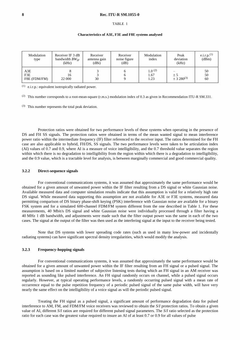
Representative AM and FM voice systems were selected for analysis. A 600-channel FDM/FM system, for

which measured performance degradation data had been obtained, was also used in the analysis. The significant

characteristics of systems used in the subsequent analysis are given in Table 1.

8 Rec. ITU-R SM.1055-0

TABLE 1

Characteristics of A3E, F3E and F8E systems analysed

(1) e.i.r.p.: equivalent isotropically radiated power.

(2) This number corresponds to a root-mean-square (r.m.s.) modulation index of 0.3 as given in Recommendation ITU-R SM.331.

(3) This number represents the total peak deviation.

Protection ratios were obtained for two performance levels of these systems when operating in the presence of

DS and FH SS signals. The protection ratios were obtained in terms of the mean wanted signal to mean interference

power ratio within the intermediate frequency (IF) filter referenced to the receiver input. The ratios determined for the FH

case are also applicable to hybrid, FH/DS, SS signals. The two performance levels were taken to be articulation index

(AI) values of 0.7 and 0.9, where AI is a measure of voice intelligibility, and the 0.7 threshold value separates the region

within which there is no degradation to intelligibility from the region within which there is a degradation to intelligibility,

and the 0.9 value, which is a tractable level for analysis, is between marginally commercial and good commercial quality.

3.2.2 Direct-sequence signals

For conventional communications systems, it was assumed that approximately the same performance would be

obtained for a given amount of unwanted power within the IF filter resulting from a DS signal or white Gaussian noise.

Available measured data and computer simulation results indicate that this assumption is valid for a relatively high rate

DS signal. While measured data supporting this assumption are not available for A3E or F3E systems, measured data

permitting comparison of DS binary phase-shift keying (PSK) interference with Gaussian noise are available for a binary

FSK system and for a simulated 600-channel FDM/FM system different from the one described in Table 1. For these

measurements, 40 Mbit/s DS signal and white Gaussian noise were individually processed through a filter having a

40 MHz 1 dB bandwidth, and adjustments were made such that the filter output power was the same in each of the two

cases. The signal at the output of the filter was then used as the interfering signal at the input to the receiver being tested.

Note that DS systems with lower spreading code rates (such as used in many low-power and incidentally

radiating systems) can have significant spectral density irregularities, which would modify the analysis.

3.2.3 Frequency-hopping signals

For conventional communications systems, it was assumed that approximately the same performance would be

obtained for a given amount of unwanted power within the IF filter resulting from an FH signal or a pulsed signal. The

assumption is based on a limited number of subjective listening tests during which an FH signal in an AM receiver was

reported as sounding like pulsed interference. An FH signal randomly occurs on channel, while a pulsed signal occurs

regularly. However, at typical operating performance levels, a randomly occurring pulsed signal with a mean rate of

occurrence equal to the pulse repetition frequency of a periodic pulsed signal of the same pulse width, will have very

nearly the same effect on the intelligibility of a voice signal as will the periodic pulsed signal.

Treating the FH signal as a pulsed signal, a significant amount of performance degradation data for pulsed

interference to AM, FM, and FDM/FM voice receivers was reviewed to obtain the S/I protection ratios. To obtain a given

value of AI, different S/I ratios are required for different pulsed signal parameters. The S/I ratio selected as the protection

ratio for each case was the greatest value required to insure an AI of at least 0.7 or 0.9 for all values of pulse

Modulation type

Receiver IF 3 dB bandwidth BWIF

(kHz)

Receiver antenna gain

(dBi)

Receiver noise figure

(dB)

Modulation index

Peak deviation

(kHz)

e.i.r.p.(1)

(dBm)

A3E F3E F8E (FDM/FM)

8 16

22 000

03 03 30

6 6 9

1.0 (2) 1.67 1.23

– 5 3 280(3)

50 50 60

Rec. ITU-R SM.1055-0 9

width, pulse repetition frequency and off-tuning for which measurements had been performed. Therefore, these S/I

protection ratios are conservative values. The pulse widths and pulse repetition frequencies for which the data varied are

given in Table 2.

TABLE 2

Parameter ranges for pulsed interference measurements

3.2.4 Signal-to-interference ratios

The S/I protection ratios are given in Table 3, and they apply for the power in the bandwidth of the receiver.

Partly due to the conservative manner in which the SS protection ratios were obtained, the protection ratio for the SS case

is, in some cases, greater than that for the like-modulation situation. However, the large bandwidths used by the SS

systems reduce the emitted power spectral density to such an extent that typically, for the specified performance levels,

lower propagation losses are required for the SS systems versus the like-modulation systems. The protection ratios given

in this Annex for the F3E cases do not utilize pre-emphasis and de-emphasis. For the F8E-to-F8E and DS-to-F8E cases,

the protection ratios were obtained from measured performance degradation data. The protection ratios for the F8E

receiver are for an upper (worst case) channel.

TABLE 3

Signal-to-interference protection ratios (dB)*

* All of the S/I ratios are mean power-to-mean power values.

(1) Described in Table 1.

(2) Direct sequence.

(3) Frequency hopping.

Modulation type

Pulse width (s)

Pulse repetition frequency (pps)

From To From To

A3E 50, 1 000 10 400

F3E 10, 1 000 40 1 000

F8E (FDM/FM) 0.1 1 000 50 15 000

Input S/N Wanted signal AI Interference modulation

(dB) modulation(1) A3E(1) F3E(1) F8E(1) DS(2) FH(3)

45 A3E 0.7 7 21 19

0.9 13 28 31

22 F3E 0.7 6 8 19

0.9 20 15 30

55 F8E (FDM/FM) 0.7 17 15 15

0.9 22 21 21

10 Rec. ITU-R SM.1055-0

3.3 Minimum required propagation loss

The protection ratios in Table 3 were used to compute the minimum required propagation loss for each system

performance level for two types of SS signals and for a like-modulation unwanted signal. The minimum required

propagation loss is defined as the minimum value which the unwanted signal must experience to insure an AI of at least

the value specified. The two types of SS signals chosen for analysis were DS and FH/DS. For each type of SS signal, both

binary antipodal PSK and MSK were evaluated for the carrier modulation. For each of these SS signals, the e.i.r.p. was

taken to be equal to that of the like-modulation interference signal in the particular case being analysed. These values of

e.i.r.p. are given in Table 1. Two typical chip rates (10 Mbit/s and 40 Mbit/s) were considered for the DS signal, where

the term chip rate refers to the signalling speed of the spectrum spreading code sequence. The FH/DS signal was assumed

to hop among 40 equally spaced carrier frequencies with a dwell time of 100 s on each frequency. The FH/DS emission

is considered to be such that each carrier frequency occurs at a mean rate of 250 times per second. Each of two values for

the chip rate of the DS modulation was considered along with each corresponding value for the separation between

adjacent frequencies. Chip rates of 2.5 and 5 Mbit/s were used along with frequency separations of 2.25 and 4.5 MHz,

respectively, for the case of PSK modulation. For the case of MSK modulation, chip rates of 2.5 and 5 Mbit/s were used

along with frequency separations of 1.5 and 3 MHz, respectively.

The minimum required propagation loss, Lp (dB) for an AI of 0.7 or 0.9 is given by:

Lp LIF – (S/N ) – N (S/I )T (6)

where:

Lp : minimum required propagation loss

LIF : transmitted interference power within the IF filter (dBm)

S/N : mean wanted signal-to-mean Gaussian noise power ratio in the IF filter (dB)

N : mean noise power within the IF filter (dBm)

(S/I)T : signal-to-interference protection ratio, the appropriate protection ratio as given in Table 3 required for

the 0.7 or 0.9 AI score.

For the detailed derivation of the propagation loss calculations, see § 6 of this Annex.

The results of the propagation loss calculations are presented in Table 4. For the FH/DS signals in the table, the

entries in the ordered sets of five numbers represent the values of parameters (nf, tf, rf, Rc, fs),

where:

nf : number of frequencies being used

tf : dwell time (s) on each carrier frequency

rf : mean rate of occurrence in occurrences/s of each carrier frequency

Rc : chip rate (Mbit/s)

fs : separation (MHz) between adjacent carrier frequencies.

The range of emission bandwidths covered by the selected typical SS signals is very wide and should be

generally applicable. Small changes in the spread bandwidth would not lead to large changes in the minimum required

propagation loss. The separation distances corresponding to the minimum required losses given in Table 4 may be

obtained using appropriate propagation loss calculation procedures. The results in Table 4 should not be used to compare

A3E, F3E and F8E with each other due to the different wanted signal levels used in the three cases.

Rec. ITU-R SM.1055-0 11

TABLE 4

Minimum required propagation losses (dB)

(1) 3 dB emission bandwidth (the emission bandwidth to be used in determining the bandwidth over which a transmitter and receiver are co-channel).

(2) This value is with respect to the peak sideband power spectral density.

3.4 Measurement data

An experiment was conducted by the Canadian Administration in Ottawa, Canada, utilizing FH commercial

equipment operating in the 30-88 MHz band. Measurements were made to identify co-channel interference protection

criteria applicable to the land mobile service operating in the low VHF band. Specifications for the FH equipment used

are given in Table 5.

TABLE 5

Specifications of the FH equipment used

Emission bandwidth(1)

Interference

Wanted signal Type of modulation

(kHz) Type of modulation A3E F3E F8E

A1 0.7 0.9 0.7 0.9 0.7 0.9

00000 1.4(2) A3E 144 150

00000 1.5(2) F3E 163 177

000 400(2) F8E (FDM/FM) 143.6 148.6

009 000 DS/PSK 10 Mbit/s 127 134 137 144 141.6 147.6

006 000 DS/MSK 10 Mbit/s 129.1 136.1 139.1 146.1 141.6 147.6

036 000 DS/PSK 40 Mbit/s 121 128 131 138 139 145

024 000 DS/MSK 40 Mbit/s 123.1 130.1 133.1 140.1 141.2 147.2

180 000 FH/DS/PSK (40, 100, 250, 5, 4.5) 111.7 123.7 134.7 145.7 131.7 137.7

120 000 FH/DS/MSK (40, 100, 250, 5, 3) 113.7 125.7 136.7 147.7 133.7 139.7

090 000 FH/DS/PSK (40, 100, 250, 2.5, 2.25) 114.7 126.7 137.7 148.7 134.7 140.7

060 000 FH/DS/MSK (40, 100, 250, 2.5, 1.5) 116.7 128.7 139.7 150.7 136.7 142.7

Operating frequency (MHz) 30-88

Hop rate (per s) 100

No. of frequencies 256

RF bandwidth (MHz) 6.4

Adjacent frequency spacing (kHz) 25

12 Rec. ITU-R SM.1055-0

3.4.1 Signal-to-interference (S/I) protection ratios

Three commercial FM receivers, having a channel spacing of 20, 50, and 25 kHz respectively, were used in the

measurements. S/I protection ratios for co-channel operation were measured using the just perceptible (JP) and

non-intelligible (NI) degradation levels which are about equivalent to the minimum interference threshold (MINIT) and

0.3 articulation index (AI). The results are given in Table 6.

TABLE 6

Co-channel signal-to-interference protection ratios (dB)

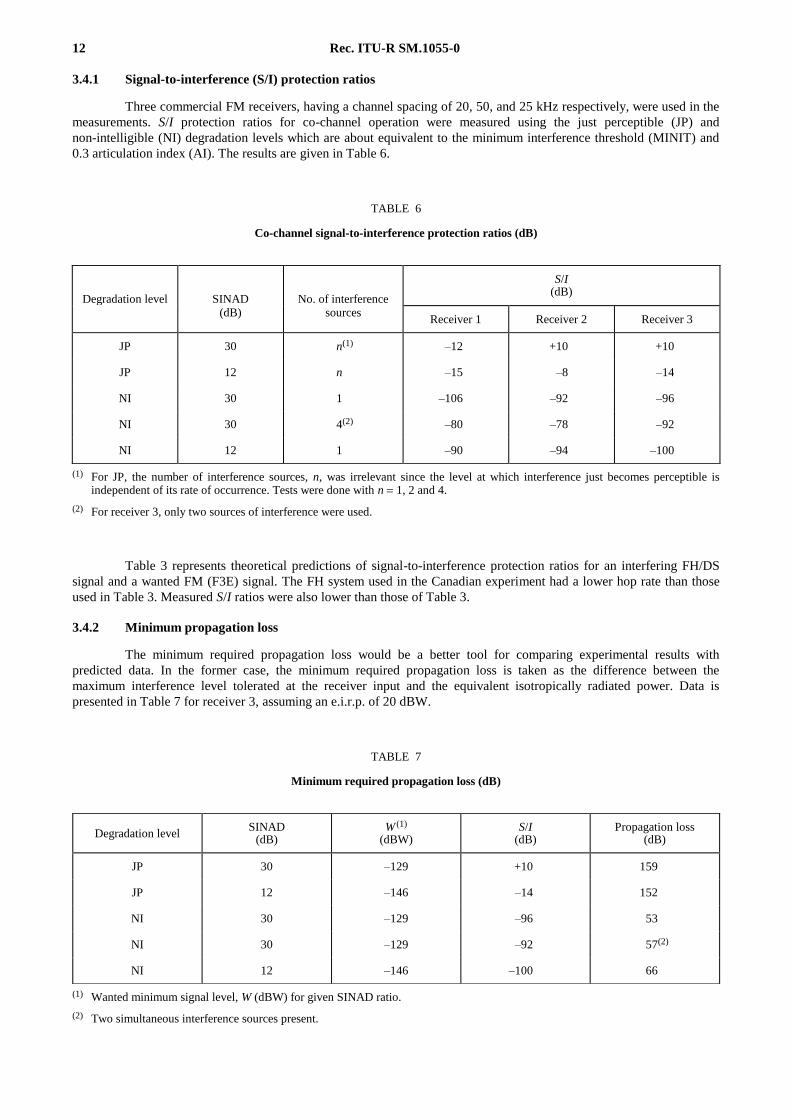
(1) For JP, the number of interference sources, n, was irrelevant since the level at which interference just becomes perceptible is independent of its rate of occurrence. Tests were done with n 1, 2 and 4.

(2) For receiver 3, only two sources of interference were used.

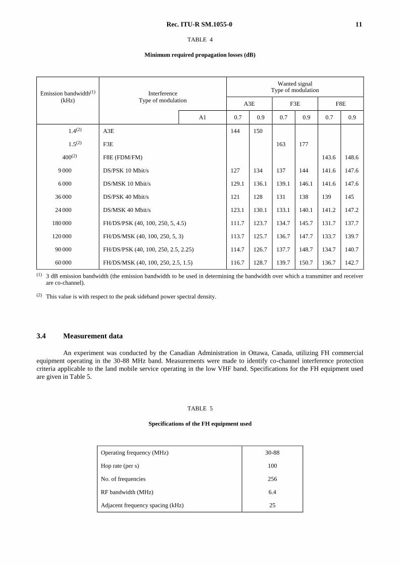
Table 3 represents theoretical predictions of signal-to-interference protection ratios for an interfering FH/DS

signal and a wanted FM (F3E) signal. The FH system used in the Canadian experiment had a lower hop rate than those

used in Table 3. Measured S/I ratios were also lower than those of Table 3.

3.4.2 Minimum propagation loss

The minimum required propagation loss would be a better tool for comparing experimental results with

predicted data. In the former case, the minimum required propagation loss is taken as the difference between the

maximum interference level tolerated at the receiver input and the equivalent isotropically radiated power. Data is

presented in Table 7 for receiver 3, assuming an e.i.r.p. of 20 dBW.

TABLE 7

Minimum required propagation loss (dB)

(1) Wanted minimum signal level, W (dBW) for given SINAD ratio.

(2) Two simultaneous interference sources present.

Degradation level SINAD No. of interference

S/I (dB)

(dB) sources

Receiver 1 Receiver 2 Receiver 3

JP 30 n(1) –12 +10 +10

JP 12 n –15 –8 –14

NI 30 1 –106 –92 –96

NI 30 4(2) –80 –78 –92

NI 12 1 –90 –94 –100

Degradation level SINAD

(dB) W

(1) (dBW)

S/I (dB)

Propagation loss (dB)

JP 30 –129 +10 159

JP 12 –146 –14 152

NI 30 –129 –96 053

NI 30 –129 –92 057(2)

NI 12 –146 –100 066

Rec. ITU-R SM.1055-0 13

The comparison between the above results, using the JP and NI degradation levels, and that of Table 4

indicated that propagation losses are slightly higher for JP than for an AI of 0.9 and lower for NI than for an AI of 0.7.

3.4.3 Summary

The experimental evidence indicates that large propagation losses are required to protect an FM receiver

against the perceptible level of co-channel interference, but on the other hand, surprisingly small propagation losses are

required to protect against non-intelligible harmful interference. Moreover, considering that actual land mobile users of

the 30-50 MHz band use analogue transmission techniques, an interference of 10 ms duration such as the one used in the

experiment, will not be annoying if it does not occur too often. For a given land mobile channel, interference from one

source was present on average 0.4% of the time so that a land mobile system (analogue voice) can tolerate a greater

number of FH sources, the maximum number being determined by the desired grade of service.

This experiment did not attempt to evaluate the impact of FH interference on digital systems nor did it study the

relationship between the number of FH interference sources and the degradation of a land mobile signal.

3.5 Conclusion

The results of this example show that lower propagation loss values are typically required for co-channel SS

systems versus like-modulation systems for both a quality which represents the threshold of intelligibility degradation and

a quality which is between marginally commercial and good commercial quality. As indicated by the results in Table 4,

the reduction in minimum required propagation loss ranged from 13.9 to 23.3 dB for the A3E system, 23.3 to 39 dB for

the F3E system and 1 to 11.9 dB for the F8E system. This indicated that a potential for sharing exists. Further

examination is required to determine detailed sharing criteria for the cases examined where a single additional radio

channel is overlaid upon a conventional radio channel. Additional cases require examination to determine the maximum

multi-system capacity that could be achieved in a given volume. Test results using a 100 hop/s FH system indicate that S/I

ratio and propagation losses required to protect conventional voice systems may be lower than predicted by theoretical

models.

Some FH signals used for land mobile applications can have channel occupancy times up to 100 ms, and other

low power FH systems can have occupancy times up to 400 ms. These types of SS systems require further analysis for

sharing. Furthermore, the analysis considered only impairment of audio quality. Further consideration needs to be given

to the interference created by repetitive breaking of squelch on conventional voice systems.

4. Example 2 – Interference from SS systems to the television broadcast service

4.1 General

The example investigates the interference from SS systems to television reception. The general type of SS

technique of interest in this example is the FH technique.

For a specified level of performance, this Annex provides S/I power ratios required for the protection of

television video and audio signals in the presence of FH interfering signals. The results are compared to situations in

which degradation of the video and audio signals due to a fixed frequency interference source is experienced. It is shown

that for co-channel and adjacent channel interference, lower protection ratios are required against unwanted FH signals

than against fixed frequency interference sources.

4.2 Frequency hopping signals

Interference tests were carried out in Ottawa, Canada, on five standard North American television receivers

using NTSC modulation. Specifications for the FH equipment used are given in Table 5. Tests were conducted in the

50-88 MHz band.

14 Rec. ITU-R SM.1055-0

4.3 Signal-to-interference (S/I) protection ratios

S/I protection ratios for co-channel and adjacent channel interference were measured using the JP and NI

degradation levels, which are about equivalent to impairment 4.5 and less than 1 respectively on the impairment grade

scale of Recommendation ITU-R BT.500. The wanted television signal level was adjusted in all tests to 49 dB(V)

across a 300 termination.

4.3.1 Co-channel interference

Co-channel interference test results are given in Table 8. Average (for five receivers) and worst case required

S/I ratios are given for television channel 6 (82-88 MHz). Other television channels required similar S/I ratios. In every

case, interference was much more severe on the video signal than on the audio signal.

TABLE 8

Television co-channel signal-to-interference ratios (dB)

These results show that television reception is less susceptible to co-channel interference from FH systems than

from narrow-band systems operating on a frequency close to, or at, the picture carrier or the colour sub-carrier.

4.3.2 Adjacent channel interference

Table 9 summarizes the results of adjacent channel interference tests. Average and worst case S/I ratios are

given for three modes of interference:

Mode 1 – lower adjacent channel;

Mode 2 – lower second adjacent channel;

Mode 3 – upper adjacent channel.

Degradation of the audio signal was, in every case, much less severe than degradation of the video signal and is

omitted in the table.

TABLE 9

Television adjacent channel signal-to-interference ratios (dB)

Degradation level No. of interfering Video Audio

sources

Average Worst Average Worst

JP 1 44 44 18 20

JP 4 46 48 22 22

NI 1 11 14 06 08

Degradation No. of interfering Mode 1 Mode 2 Mode 3

level sources Average Worst Average Worst Average Worst

JP 1 –3 1+8 –18 –5 –30 –27

JP 4 1 11 –13 –0 –23 –18

Rec. ITU-R SM.1055-0 15

It is reported in ex-CCIR Recommendation 418 (Geneva, 1982) that protection ratios considered to be

acceptable when one interference source is present less than 10% of the time are –6 dB for lower adjacent channel

interference and –12 dB for upper adjacent channel interference. Protection ratios for just perceptible degradation are

said to be 10-20 dB higher. Assuming that an FH system does not create interference to a television receiver more than

10% of the time, then Table 9 results are an improvement over figures in ex-CCIR Recommendation 418 (Geneva, 1982).

4.4 Conclusion

The results of this example show that, for a given grade of service at television receiver input, lower S/I ratios

were required for co-channel and adjacent channel FH emissions than from fixed frequency emissions. This example

indicates that a potential for sharing exists, especially in adjacent channel operations. Further examination is required to

determine the relationship between the required S/I ratio and the number of FH transmissions applicable to various

situations, as well as to explore the capabilities of FH systems to avoid transmissions at frequencies near or at the picture

and colour television carriers. These results do not apply to digital or high-definition TV systems, which are expected to

behave very differently in the presence of interference. Spread spectrum sharing considerations must wait for more

information on technical characteristics and deployment plans for these new television systems.

5. Summary

In the first example, for system performance levels of 0.7 and 0.9 articulation index, signal-to-interference

protection ratios were given for A3, F3 and F8 (FDM-FM) voice communication systems operating in the presence of

like-modulation and SS signals. Direct-sequence, FH and hybrid FS/DS SS signals were considered. For a

like-modulation signal and several SS signals of the same radiated power, the minimum required propagation losses for

the acceptable performance of the A3, F3 and F8 systems were tabulated. The results for these cases show that lower

propagation loss values are typically required for co-channel SS systems versus like-modulation systems for both a

quality which represents the threshold of intelligibility degradation and a quality which is between marginally commercial

and good commercial quality. Test results for an FH system substantiated the above results. Just perceptible and non-

intelligible degradation levels were used in the tests.

The second example deals with the interference from FH systems to television reception in the low VHF band.

Test results indicate that lower protection ratios are required for co-channel and adjacent channel FH systems versus fixed

frequency systems for a just perceptible degradation level.

The above examples show that with careful consideration of design factors, a potential for band sharing exists

between SS and other modulation techniques.

6. Calculation of minimum required propagation loss

The minimum required propagation loss, Lp (dB) for an AI of 0.7 or 0.9 is given by:

Lp IIF – (S/N ) – N (S/I )T

Lp IIF – (S/N ) 174 – 10 log BWIF – NF (S/I )T (7)

where:

N : mean noise power within the IF filter (dBm)

BWIF : filter 3 dB bandwidth (Hz).

(For the definition of other terms, see § 3.3.)

16 Rec. ITU-R SM.1055-0

For the like-modulation interference, all of the transmitted power is contained within the IF filter so that IIF may

be expressed as:

IIF IE + GR (8)

where:

IE : e.i.r.p. of the interfering system (dBm)

GR : antenna gain of the receiving system (dBi).

For the DS interference, IIF is given by:

IIF IE GR – FDR(0) (9)

where FDR(0) is the frequency dependant rejection (dB) for f 0 and FDR( f) is defined by Recommenda-

tion ITU-R SM.337 as:

FDR ( f ) = 10 log

0

P( f ) df

0

P( f ) H( f f ) df

(10)

where:

p( f ) : emission spectral density (within a multiplicative constant) of the interfering signal

H( f ) : receiver selectivity function due to all filters up to and including the IF filter

f : difference between the carrier frequency of the interfering signal and the receiver tuned frequency.

For the FH/DS interference, the expression for IIF becomes:

IIF IE GR 10 log (f rf) 10 log i 1

nfi

1

FDR ( fi) (11)

where:

tf : dwell time (s) on each carrier frequency

rf : mean rate of occurrence in occurrences/s of each carrier frequency

nf : number of frequencies being used and FDR( fi) may be obtained from:

FDR ( fi) 10FDR ( fi) / 10 (12)

where fi is the difference between the ith carrier frequency of the FH/DS interfering signal and the receiver tuned

frequency.

The normalized power spectrum (i.e., unity maximum power spectral density) for binary PSK is given by:

p( f ) = sin2

( f / Rc)

( f / Rc)2 (13)

and that for MSK is given by:

p( f ) 1 cos (4 f / Rc)

2

1

– 16 ( f / Rc)

2 2 (14)

where Rc is the chip rate.

The results of the propagation loss calculations are presented in Table 4.

Rec. ITU-R SM.1055-0 17

ANNEX 3

Procedures for analysing spread spectrum

interference to conventional receivers

1. Introduction

This Annex presents procedures that can be used to quantify the interactive effects between spread-

spectrum (SS) interferers and conventional receivers. The procedures extend the use of the frequency-dependant-rejection

(FDR) concept for calculating the frequency distance (FD) separation, which is described in Recommendation ITU-R

SM.337. The FDR and FD are measures that aid the solution of co-channel frequency sharing and adjacent band

interference problems by providing minimum frequency and distance separation criteria between interferer and receiver

for acceptable receiver performance.

A detailed description of SS modulation techniques is given in Annex 1. The two general types of SS signalling

techniques that are of interest here are direct-sequence (DS) and frequency-hopping (FH). The hybrid forms employing

both of these methods (FH/DS) and time-hopped DS (TH/DS) modulation are also of interest.

2. General approach

In Recommendation ITU-R SM.337, a procedure is given for computing an FD curve, which is based on the

inequality:

Lb (d ) FDR ( f ) Pt Gt Gr – Im (15)

where:

Lb(d) : basic transmission loss for a separation distance d between interferer and receiver (dB)

Pt : interferer transmitter average power (dBm)

Gt : gain of interferer antenna in direction of receiver (dBi)

Gr : gain of receiver antenna in direction of interferer (dBi)

Im : maximum allowed average interference power to prevent unacceptable performance (dBm)

FDR( f ) : defined by equation (2) in Recommendation ITU-R SM.337 (dB).

Inequality (15) is applicable when the unwanted emission is continuous in time and produces a response

waveform that is continuous in time. When the emission is frequency-hopped or time-hopped, it produces a response

waveform that may not be continuous in time, and the performance is dependant on the peak rather than the average

interference power. For that condition, inequality (15) is replaced by:

Lb (d ) + FDR ( f ) Pt Gt + Gr – Îm (16)

where:

Pt : interferer transmitter peak power (dBm)

Îm : maximum allowed peak interference power to prevent unacceptable performance (dBm).

The function FDR ( f ), which is used when peak interference levels are involved is obtained by:

FDR ( f ) FDR ( f ) i – 0 ( f ) (17)

18 Rec. ITU-R SM.1055-0

Expressions for the terms i, the duty cycle of the unwanted emissions waveform at the receiver input, and

0( f ), the duty cycle of the response waveform, are given in Table 10. These expressions are applicable to gated digital

signals and can be used also when the responses to the SS emission consist of impulses or bursts.

TABLE 10

Duty-cycle functions for interfering digital signals

(2-PSK, 4-PSK, MPSK, O4-PSK, MSK, 2-FSK)

MPSK: M-ary phase shift keying

2-PSK: binary phase shift keying

4-PSK: quadriphase shift keying

O4-PSK: offset 4-PSK

MSK: minimum shift keying

2-FSK: binary frequency shift keying

Br : 3 dB bandwidth (Hz) of the receiving channel

Rs : symbol rate (Bd) of a digital interferer

g : gate length (s) of time gated interferer signal

Tg : average spacing (s) of gates

: pulse length (s)

d : smoothing function.

After all of the terms except Lb(d) have been calculated using the procedure given in the following sections,

an FD curve can be obtained using the procedures given in Recommendation ITU-R SM.337. The primary subject of this

Annex is the procedures that are used to calculate Im and Îm as required for the various types of SS emissions.

3. Response waveform considerations

The response waveforms produced by emissions involving digital signalling take a number of different forms

that depend on the characteristics of the interfering signal and the selectivity of the receiver. The procedure required to

compute the peak interference levels and FD for a particular type of SS emissions depends on the type of the response

waveform that is produced. Table 10 gives expressions to calculate i and 0( f ) for various bandwidth conditions for

interfering digital signals.

Continuous input waveform i 0 dB

Bandwidth conditions 0 ( f )

(dB)

Br /Rs 1, f 0

Br /Rs 1, f Br / 2

Br /Rs 1, f Br / 2

0

0

–d ( f ) 10 log (2 Br /Rs)

Gated input waveform i 10 log (g/ Tg) dB

Bandwidth conditions 0 ( f )

(dB)

Br /Rs 1, 1/Br g, f 0

Br /Rs 1, g 1/Br Tg, f 0

Br /Rs 1, 1/Br g, f 0

Br /Rs 1 f Br / 2

Br /Rs 1 f Br / 2

10 log (g/ Tg)

10 log 1/(Br / Tg)

0

10 log (g/ Tg)

10 log (g/ Tg) – d ( f ) 10 log (2 Br /Rs)

Rec. ITU-R SM.1055-0 19

As f is increased from 0 to Br /2, the response waveform changes. For purposes of simplification in

calculating 0( f , arbitrary smoothing functions are used to account for the transitional wave shape that occurs when

f Br /2.

The smoothing function d ( f ) for digital signals is:

d ( f ) 1 – exp

– d

f

Br –

1

2 for f Br / 2 (18)

where:

d 3.91/( fd /Br) – (1/2))

fd : frequency at the intersection of 10 log H( f ) and 10 log P( f ) 20 log (Br /Rs) – 10.

If 10 log H( f ) exceeds the other expression for all values of so that there is no intersection,

d ( f ) 0.

where:

H( f ) : receiver selectivity

P( f ) : normalized interferer emission spectra density.

3.1 Noise-like response, continuous in time

When the response is noise-like and continuous in time, which occurs when a receiver is subjected to a DS

emission that has a bandwidth greater than the bandwidth of the receiver, the interference can be considered as additional

receiver noise. The effects on the receiver performance can be determined using a measure that is appropriate for noise

interference.

3.2 Response continuous in amplitude and time

A response that is continuous both in amplitude and time is produced by a co-channel DS emission when the

receiver bandwidth is greater than the instantaneous emission bandwidth.

3.3 Impulsive and burst responses

Some types of SS emissions, namely TH/DS, FH, and FH/DS, usually produce responses that consist of

randomly spaced impulses or noise bursts. Also, adjacent channel interference from DS emissions produces randomly

spaced impulses when the receiver bandwidth is greater than the emission bandwidth.

Table 10 gives equations for calculating the input and output waveform duty cycles, i and 0( f ) respectively,

for various bandwidth conditions. The fraction of time that the response waveform is non-zero is denoted by DC, which is

approximated by:

DC antilog [0.1 0 ( f)] (19)

When the response waveform consists of short bursts and has a low duty cycle, signal-to-peak interference

ratios S/Î much less than 0 dB can be tolerated. For example, with experienced listeners, the intelligibility as measured by

articulation score in an AM voice transmission subjected to radar pulses is not reduced even when S/Î –70 dB if the

duty cycle of the incoming pulse is less than 8%. Other observations indicate that to avoid listener annoyance, the duty

cycle of a response consisting of noise bursts should not exceed about 5%. Although criteria are available for interference

involving pulses that are of the order of 1 s long, criteria that are applicable to the lower burst lengths that are typical of

intermittent SS interference have not been published.

Guidelines for determining Îm when interference produces intermittent responses are given in Table 11 for AM

voice receivers, Table 12 for FM voice receivers, and Table 13 for conventional digital receivers. Note from the tables

that the receivers must be protected from several types of interference mechanisms, namely: listener annoyance, loss of

intelligibility, excessive probability of symbol error, impairment of the automatic gain control, and impairment of the

synchronization process.

20 Rec. ITU-R SM.1055-0

TABLE 11

Guidelines for determining Îm for intermittent* interference in AM voice receiver

* Included responses to TH/DS, FH and FH/DS emissions.

B : length of interference bursts (s).

DC : duty cycle of interference response (%).

TABLE 12

Guidelines for determining Îm for intermittent interference in FM voice receivers

TABLE 13

Guidelines for determining Îm for intermittent interference in conventional digital receivers

tB : length of interference bursts (s).

Tu : AGC attack time (s).

Ts : synchronization break time (s).

Conditions Requirement Procedure

B 1 ms and DC 5% Prevent loss of intelligibility Use procedures given in § 4.3.2 or 4.4.2

B 1 ms and DC 5% Prevent listener annoyance Treat as if the duty cycle were 100%

B 1 ms Prevent impairment to AGC Treat as if the duty cycle were 100%

Type of emission Conditions Requirement Procedure

TH/DS DC 5% and B 100 ms Prevent loss of intelligibility Use procedures given in § 4.3.3

TH/DS DC 5% Prevent listener annoyance Treat as if DC 100%

FH or FH/DS B 100 ms Prevent listener annoyance Use procedure given in § 4.4.3

FH or FH/DS B 100 ms Prevent listener annoyance or loss of intelligibility

Use procedure given in § 4.4.3

Conditions Requirements Procedures

B Tu and B Ts Prevent unacceptable probability of symbol error

Use procedures given in § 4.3.1 or 4.4.1

B Tu Prevent impairment of AGC Treat as if the duty cycle were 100%

B Ts Prevent impairment to synchronization process

Treat as if the duty cycle were 100%

Rec. ITU-R SM.1055-0 21

4. Procedures for determining Îm

4.1 General

A general expression for obtaining Îm is:

Îm N0 10 log (10MI / 10 – 1) (20)

where N0 is receiver noise, given by:

N0 10 log kT0 10 log BWIF (Hz) + noise figure (21)

MI is the interference margin, given by:

MI (S/N )0 – (S/I )i (22)

where:

(S/N)0 : signal-to-noise ratio (dB) when the receiver is not subjected to an unwanted emission

(S/N)i : signal-to-(noise-plus-interference) ratio (dB) when the receiver is subjected to the SS emission.

In some interference analysis either (S/N)0 and (S/N)i, or MI may be specified. In other analyses, the

performance in the absence of interference and the minimum allowed performance in the presence of interference are

specified. For voice transmissions, the articulation score (AS) is the performance measure; AS0 denotes the AS in the

absence of interference. For digital transmissions, the probability of symbol error (Pe) is the performance measure; Pe,0

denotes Pe in the absence of interference, Pe,i, denotes Pe in the presence of interference, and Pe,I denotes the probability

of error of symbols that are coincident in time with an impulse or burst response produced by SS.

4.2 Procedure used for DS emissions

A DS emission produces a response that is continuous in time when the emission bandwidth exceeds the

receiver bandwidth. For that condition, inequality (15) and the procedures in Recommendation ITU-R SM.337 are used

to determine Im and FD. As it is very unlikely that the bandwidth of a DS emission will be less than the bandwidth of an

AM-voice receiver, the procedure for that condition is not included here. For a digital receiver with a bandwidth that

exceeds the DS emission bandwidth, the procedure given in § 4.3.1 is applicable. In using equation (19) to calculate DC,

0( f ) is obtained from Table 10 using the equation that is appropriate for a continuous input waveform.

4.3 Procedure used for FH/DS emissions

An important characteristic of the response waveforms produced by SS emissions is the fraction of time the

amplitude of the response waveform is non-zero. An approximation of that fraction is the output duty-cycle 0( f ) which

is a function of g, Tg, Br and f . Table 10 defines 0( f ) and lists expressions that can be used to calculate that function

for responses produced by FH/DS emissions.

4.3.1 Digital receivers

For digital receivers, determination of Îm entails first determining Pe,I using the relationship:

Pe,I Pe,i

DC

–1( f ) Pe,0[1 – DC –1( f )] (23)

After Pe,I has been calculated, the corresponding interference level that yields Pe,I is determined. When the

response is noise-like, a curve or expression for Pe(S/N) is used to determine (S/N)i. When the response is CW-like,

i.e. continuous in amplitude, a curve or expression for Pe(S/N, S/I) is used to determine S/Î. Îm is then obtained by:

Îm = (S/N )0 – (S/Î ) + N0 (24)

where (S/N)0 is determined using a curve of Pe(S/N), i.e. (S/N)0 is the signal-to-noise ratio that yields the specified value

of Pe,0. The receiver noise N0 is obtained using equation (21).

22 Rec. ITU-R SM.1055-0

Having determined both (S/N)i and (S/N)0, MI is calculated using equation (22), and then Îm can be obtained

using equation (20).

4.3.2 AM voice receivers

For AM voice receivers, Îm is determined using the expression:

Îm = 10 log

(S/N )0

(S/N )i – 1

N0

DC ( f ) (25)

where:

(S/N)0 : signal-to-noise ratio that yields AS0

(S/N)i : signal-to-(noise plus interference) ratio that yields ASi.

Note 1 – None of the ratios or terms in the brackets are in dB.

Curves of the AS as a function of white Gaussian noise interference can be found in Fig. 1.

B

A

D

C

0

10

20

30

40

50

60

70

80

90

100

– 20 – 10 0 10 20 30 40 45

D01

FIGURE 1

Articulation score as a function of noise interference

Art

icu

lati

on

sco

re (

%)

phonetically balanced word groupings: 50

white-noise bandwidth 6 kHz

phonetically balanced word groupings: 1 000

white-noise bandwidth 3 kHz

A:

B:

C:

D:

Output signal-to-interference ratio (S/I) (dB)0

FIGURE 1/SM.1055...[D01] = 15 CM

Rec. ITU-R SM.1055-0 23

4.3.3 FM voice receiver

When an FM voice receiver is subjected to a TH/DS emission which produces a response with a peak power

greater than the desired signal power, the performance is dependant on the duty cycle of the response waveform rather

than on the average or peak power. When B 100 ms, unacceptable degradation will not occur if:

(1 – DC ) 100 ASi (26)

where:

B : burst length of the response

ASi : minimum allowable articulation score.

To prevent listener annoyance, DC should not exceed 0.05 (5%). If DC exceeds 0.05, then the TH/DS emission

should be treated as if the emissions were continuous in time which results in DC 1.0. For that case, Îm Im, and the

procedures given in Recommendation ITU-R SM.337 which applies to emissions that are continuous in time, should be

used.

4.4 Procedure used with FH and FH/DS emissions

The maximum allowed interference power for FH emissions is determined using a trial and error procedure.

The peak power of the interference response, Î( fi), associated with each frequency in the hop set used by the FH emitter

is determined by:

Î ( fi ) Îa – FDR ( fi), j 1, 2, ..., NF (27)

where Îa is a chosen value for the maximum allowed peak interference at the receiver input (at the output of the receiving

antenna). As will be seen from the discussion that follows, the correct value for Îa is found by trial and error. FDR ( fi) is

obtained using equation (17), NF is the total number of frequencies in the hop set, and:

fi fr – fj (28)

where:

fr : tuned frequency of receiver (Hz)

fj : jth frequency in the hop set used by the FH emitter (Hz).

4.4.1 Digital receivers

When the response is noise-like, the probability of error Pe,j for symbols that are coincident in time with an

interference burst or impulse associated with the jth frequency in the hop set is a function of (S/N)j, which is obtained by:

(S/N )j = (S/N )0

1 + Î ( fj)

N0

, j = 1, 2, ..., NF (29)

where N0 is determined using equation (21) and converting from dBm to mW.

Note 1 – None of the terms of equation (29) are in decibels.

When the response is CW-like, Pe,j is a function of (S/N)0 and S/Î ( f j) where:

S/Î ( fj) (S/N )0 – Î ( fj) N0 (30)

24 Rec. ITU-R SM.1055-0

The expected probability of symbol error Pe for the value selected for Îa is given by:

Pe = 1

NF

j 1

NF

Pe,j f ( fi) Pe,0 [1 – f ( fj)] (31)

where:

f ( f ) (0 / f ) DC ( f ) (32)

0 : half-power burst length and

f : frequency dwell time, which is equal to the reciprocal of the hopping rate Rh.

As shown in Fig. 2, the transmitter is off during an interval of length 0 when the frequency is changed. After Pe has been

calculated, it is compared to Pe,i. If Pe Pe,i, a different value is chosen for Îa and the computations involving equations

(27), (29), (30) and (31) are repeated. If Pe Pe,i, the value that was chosen for Îa and used in equation (27) is the

maximum allowed peak interference level at the receiver input.

The receiver performance is acceptable only if:

Lb (d ) Pt Gt Gr – Îa (33)

Using Lb(d) obtained from above, the required distance separation can be determined using the procedure given

in Recommendation ITU-R SM.337. To calculate an FD curve, different values are selected for fr (see equation (27)) and

the above process is repeated for each value of fr.

4.4.2 AM voice receivers

For AM voice receivers, the articulation score is dependant on the average interference power I in the receiver

bandwidth, for the conditions that were given in Table 1. After a value is chosen for Îa and equation (26) is used to

calculate Î( f j), j 1, 2, ..., NF, the average interface power is obtained by:

I = 1

NF

j 1

NF

f ( fj) · antilog [0.1 Î ( fj)] (34)

where f ( fj) is obtained with equation (32). The maximum allowed average interference power Im is obtained by:

Im =

(S/N )0

(S/N )i – 1 N0 (35)

where N0 is obtained using equation (21) and converted from dBm to mW. It is assumed here that ASi 70%: for that

condition, the maximum allowed peak power of the response will be less than the clipping level of the audio amplifier.

Note 1 – None of the terms of equation (35) are in decibels.

If Ie Im, a different value is chosen for Îa and the computations involving equations (27) and (34) are

repeated. If Ie Im, the value chosen for Îa is the maximum allowed peak interference at the receiver input. Îa is then used

in inequality (33) to determine the minimum allowed value for Lb(d). The required distance separation is determined

using the procedure given in Recommendation ITU-R SM.337. To compute an FD curve, different values are selected for

fr (see equation (28)) and the process given above is repeated for each value of fr.

4.4.3 FM voice receiver

For voice receivers subjected to FH or FH/DS emissions, the performance is dependant on the duty cycle of the

response rather than the average or peak power when the peak power of the interference response exceeds S –3 dB, where

S is the wanted signal.

When B 100 ms, inequality (26) must be satisfied to prevent unacceptable degradation.

Rec. ITU-R SM.1055-0 25

When B 100 ms, DC must not be allowed to exceed 5%, otherwise listener annoyance will occur. That duty

cycle requirement is satisfied when:

Nc 0.05 NF · f 0 (36)

where:

Nc : maximum number of frequencies (within the hop set used by the emitter) for which Î S – 3

Î : peak power of the IF response waveform

S : wanted signal power

NF : total number of frequencies in the hop set

f : dwell time on each frequency and

0 : effective time the power is at peak value during the dwell time (see Fig. 2).

0

r f

0

2

0

2

t

f

100%

50%

0

FIGURE 2

Envelope of an FH emission

Po

wer

D02

frequency dwell time

rise time

fall time

dead time

f

r

f

0

:

:

:

:

FIGURE 2/SM.1055...[D02] = 12 CM

The interference waveform will have a duty cycle of 5% or less when the following inequality is satisfied:

Lb (d ) FDR ( fx ) PI GI Gr – Îm (37)

where:

Îm S – 3 (38)

fx max

fh –

NF

2 – Nc fc,

Nc

2 fc (39)

fc : spacing between the frequencies in the hop set (Hz), the spacing is assumed to be uniform,

fh f r – ff, and fh is the centre of the frequency-hopping band.

26 Rec. ITU-R SM.1055-0

If parameters of the emission and receiver are such that a duty cycle of 5% or less cannot be attained, if for

example NF 20, then the emission should be treated as if it were continuous, i.e. DC 100%. For that case, Îm Im, and

the procedures in Recommendation ITU-R SM.337 which apply to emissions that are continuous in time, should be used.

5. Conclusions

Procedures have been given for computing the maximum allowed interference power in receiver responses

produced by a class of SS emissions. The computed value can be used to compute the frequency and distance separations

required between the SS interferer and a conventional receiver. These computations are required for sharing problems

involving co-channel and adjacent channel interference. If the computation of required distance separation results in a

distance short enough to be considered as a co-site condition, additional co-site interference computations should be

made. The analyses presented are relative to subjective judgements of annoyance and intelligibility impairment. Other

manifestations of interference such as squelch-breaking of conventional voice systems need to be considered in further

studies.