RECCE

An Inventory Method For Describing

New Zealand Vegetation:

A Field Manual

R.B. Allen

Manaaki Whenua - Landcare Research P.O. Box 69 Christchurch

2

CONTENTS

ABSTRACT......................................................................................................................... ......3 1. INTRODUCTION.............................................................................................................4 2. OBJECTIVES....................................................................................................................6 3. INVENTORY DESIGN ....................................................................................................6

3.1 LOCATION OF RECCE DESCRIPTIONS............................................................6 3.1.1 Representative sample of study area..........................................................7 3.1.2 Stratified sample of study area...................................................................8 3.1.3 Subjective sample of study area.................................................................8

3.2 RECCE DESCRIPTION SAMPLING INTENSITY ..............................................8 4. RECONNAISSANCE (RECCE) DESCRIPTION PROCEDURE...................................9

4.1 IDENTIFICATION INFORMATION.....................................................................9 4.2 SITE CHARACTERISTICS..................................................................................10 4.3 VEGETATION PARAMETERS...........................................................................12 4.4 INCIDENTAL INFORMATION ..........................................................................12 4.5 HEIGHT-TIER INFORMATION .........................................................................13

5. DATA STORAGE...........................................................................................................15 5.1 RECCE DESCRIPTION SHEETS ........................................................................15 5.2 MAPS AND AERIAL PHOTOGRAPHS .............................................................15

6. ACKNOWLDEGEMENTS ............................................................................................16 7. REFERENCES................................................................................................................16

APPENDIX 1 : Reconnaissance (Recce) Description Sheet...........................................19 APPENDIX 2 : Equipment List ......................................................................................21

3

SUMMARY Effective management of New Zealand’s diverse vegetative cover requires a field method for describing its compositional variation and the distribution of individual component species. The Reconnaissance (Recce) description procedure is widely used for this purpose, and this manual updates and standardises the method. Random, systematic, stratified, and subjective sampling schemes are outlined for the location of Recce descriptions, the choice of which depends upon specific objectives. Each Recce description includes a species list in height tiers, with associated cover estimates, and records site characteristics and additional vegetation parameters. Much of the Recce description data collected so far is stored in the ‘National Indigenous Vegetation Survey Database’, held by the Forest Research Institute, Christchurch (from mid-1992 the Crown Research Institute for Land Environments, Christchurch). The analysis of such data by gradient and community based methods has emerged as a principal approach in the study of vegetation/environment relationships. KEYWORDS: Distribution; plant community analysis; sampling techniques; site factors; species composition; vegetation surveys.

4

1. INTRODUCTION

New Zealand’s land surface of c. 26.9 million hectares has a diverse vegetative cover (Newsome 1987). Effective management of this resource requires information on key characteristics such as structure, productivity, and species composition. From an environmental perspective, compositional variation in vegetation and the distribution of individual component species will often be the characteristics of interest. This manual updates and standardises an inventory method for this purpose that has been widely used in a broad spectrum of New Zealand’s vegetation. For anyone setting out to analyse compositional variation in vegetation, several alternatives are available for any specific problem. Major decisions include whether to use fixed or variable area plots and whether to use quantitative or qualitative species importance information. It is not the purpose of this manual to review alternatives, which have received comprehensive treatment in the literature (e.g., Mueller-Dombois & Ellenberg 1974; Havel 1980; Gauch 1982; Jongman et al. 1987; Økland 1990). As in most countries, during the first half of this century vegetation description in New Zealand was largely subjective. However, the development of analytical methods and the widespread availability of computers have brought about a fundamental change in the way vegetation inventories are done. Resource management decisions can now be made using results from repeatable, quantitative inventories. Increasing awareness of the environmental implications of land management has highlighted the need for such baseline information. At a national level, the first quantitative inventories of the indigenous forests were carried out by the former New Zealand Forest Service: the National Forest Survey (1945–1955) concentrated on the merchantable forests to establish timber volumes (Holloway 1956), and the Ecological Survey (started in 1958) included the non-merchantable forests to establish a classification of forests and to map forests accordingly. More recently, the Protected natural Areas Programme set out to progressively identify representative natural areas nationally, using a rapid survey methodology (Kelly & Park 1986). Numerous inventories of more limited extent have been carried out by universities and various national and local government agencies, including the Forest Research Institute (FRI). The Forest Research Institute has worked intensively on the ecology and management of montane vegetation since 1955. An important reason for initiating this work was to investigate the effects of introduced browsing animals. It was soon found that a detailed knowledge of plant community patterns was an essential framework for understanding the impact of browsing animals (e.g., Wardle et al. 1971; Wardle 1974). With this background, a methodology was designed for rapid broad-scale surveys of compositional variation in mountainland forests. This method, Reconnaissance (Recce) description, is similar to the widely used Braun-Blanquet relevé used for phytosociological analysis (see Mueller-Dombois & Ellenberg 1974). Although the Recce description

5

methodology was developed for extensive forest surveys, it has also been widely used in vegetation varying a great deal in structure and composition, including shrublands, grasslands, and mires (e.g., Rose 1985a; Norton & Leathwick 1990), and for surveys of small areas where the objectives were more specific (e.g., Leathwick 1987; Rose et al. 1988). Recce descriptions include a species list in height tiers, with associated cover estimates, records of site characteristics, and additional vegetation parameters. The analysis of such data using gradient and community based methods has emerged as a principal approach in the analysis of vegetation/environment patterns (Gauch 1982; Jongman et al. 1987). The following examples illustrate some uses of Recce data:

• Relating compositional variation in vegetation to site conditions: The relationship between alpine tussock grassland communities, landform, and soils at Wapiti Lake, Fiordland, were examined using 139 subjectively located Recce descriptions (Rose et al. 1988).

• Describing the vegetation of ecological reserves for conservation purposes: An inventory of the Waipapa Ecological Area quantified its botanical resources by describing the species and communities present and their relationship to environmental factors, using 258 Recce descriptions (Leathwick 1987).

• Analysing geographic variation in the species composition and diversity of vegetation: About 1200 Recce descriptions located throughout South Island conifer-broadleaved hardwood forests were used to compare community composition (Reif & Allen 1988); and species turnover in relation to elevation was compared for nine localities (Allen et al. 1991).

• Quantifying the basis for reserve selection (e.g., Williams et al. 1990): The number and extent of the main vegetation communities in the Mackenzie Ecological Region were surveyed to provide a framework for recommending representative conservation areas under the Protected Natural Areas Programme (Espie et al.; Myers et al. 1987).

• Determining habitat use by animals: Wardle et al. (1971) used height-tier information and browse records to determine the impact of deer in Fiordland; Spurr & Warburton (1991) assessed the method for determining habitat use by birds in Westland forests.

Much of the Recce description data collected so far (>40 000 descriptions) is now stored in the National Indigenous Vegetation Survey (NIVS) Database (Forest Research Institute 1989) held by FRI, Christchurch (from mid-1992 the Crown Research Institute for Land Environments). It is envisaged that this database will eventually develop to the point where it will provide information for a quantitative analysis of the vegetative cover of New Zealand and its relationship with the environment. This manual standardises the Recce description methodology for those wishing to use it, and updates earlier versions (Stewart & Orwin 1986; Allen & McLennan 1983; Allen &

6

McLennan 1978 (FRI unpubl. report). An updated analysis manual for such data has been written (Hall 1992). There will sometimes be sufficient reason to change aspects of the methodology for specific objectives, but collecting the standard data outlined in this manual will maximise future comparability of data. It is therefore recommended that any changes should be considered as additions to the standard methodology. Brief treatments are given, with appropriate references, for some additions previously found useful. 2. OBJECTIVES

Vegetation inventory must be based on an explicit statement of the problem and objectives (Jongman et al. 1987). A clear concise statement of the problem sets a guideline for stating objectives. A statement of objectives forms the basis for decisions about comparisons to be made as well as explanatory and response variables to be measured, which allows an efficient use of resources. This task is often complex because:

• Resource inventories are often multi-faceted and it is difficult to optimise sampling for the various objectives. If agreed objectives are not determined by all those involved, they will change and diverge during a study.

• Field sampling can lead to new issues that may result in modification of the original objectives. This may well reflect a problem statement that has not been carefully researched.

It is important that existing information is researched carefully as this will partly determine whether an inventory is justified and what the particular objectives should be. The ability to do this has been greatly enhanced by formation of the NIVS database. 3. INVENTORY DESIGN

A well thought out design is the foundation for meaningful analysis of vegetation pattern and the application of statistical tests to realise inventory objectives (see Jongman et al. 1987). The purpose of an inventory will influence the sampling strategy and hence the number and location of Recce descriptions. The strategy will also need to take account of any constraints, such as the nature of the terrain to be surveyed. 3.1 LOCATION OF RECCE DESCRIPTIONS

Recce descriptions are usually used to sample vegetation throughout a survey area. They may be located as a representative, stratified, or subjective sample of the study area. Whatever the approach, the location of all Recce descriptions should be transcribed onto aerial photographs and topographic maps. Some of the more widely used approaches to sampling with Recce descriptions are given below, along with example applications

7

3.1.1 Representative sample of study area

Representative samples of the study area can be obtained by random, restricted random, or systematic location of Recce descriptions. Such approaches are often used when the focus is resource inventory of an area. Randomised sampling eliminates systematic errors and allows the application of powerful inferential statistics (Jongman et al. 1987). However, because it is difficult to establish randomly selected plots in mountainous country, early surveys often compromised and located Recce descriptions at fixed intervals (often 100 m) on predetermined transect lines (see Allen & McLennan 1983). Starting points for such transects are selected on a restricted random basis so that recce descriptions will be representative of the area as a whole. Two methods for the placing of transect lines are often used:

(a) A grid pattern is used with the X and Y coordinates found on a NZMS Series 1 map or the NZMS Series 260 metric equivalent. If the NZMS Series 1 is used, divide the survey area in 10 000 × 10 000-yd blocks. Each block is subdivided into one hundred 1000-yd squares. Using random X and Y coordinates, choose 5–10 of these squares, depending on required sampling intensity. Identify the point on a watercourse that is nearest to the centre of the selected 1000-yd square. This point becomes the line origin. Randomly assign the transect to one side of the watercourse. Draw a line from the origin to the nearest main ridge or treeline. (b) On a map divide the survey area into blocks or catchments, then allocate the required number of lines per area. Start at either the head or the mouth of a river and run a planimeter along the main stream and all tributaries. Select a random number (usually two-figured) and stop when the planimeter reaches that number. This point is the line origin. Randomly assign the transect to one side of the watercourse.

As an example, for an inventory of 140 000 ha in the headwaters of the Grey River, Westland, 658 Recce description were located at 60-m elevation intervals along 57 transects (Wardle 1974). The data were used to classify the vegetation into plant communities and were analysed for regional patterns as well as to determine the impact of introduced browsing animals using browse records and the species/tier information. An alternative to locating Recce descriptions along transect lines is to systematically locate them on a grid system. Leathwick (1987) used this approach in a description of the Waipapa Ecological Area based on 129 descriptions located on a 500 × 500-m grid to sample the forest, 65 descriptions on a 250 × 250-m grid to sample the shrubland, and 61 descriptions on a 100 × 100-m grid to sample the mires. Although these methods give a representative sample of the study area, Recce description density is often not high enough to sample all sites of interest adequately enough to meet study objectives. Additional subjectively located Recce descriptions can be used to sample

8

extra sites, e.g., Rose’s (1985b) study of West Nelson forests (largely sampled with transects) and Leathwick’s (1987) Waipapa Ecological Area study. 3.1.2 Stratified sample of study area

With sufficient prior knowledge, the area can be stratified for efficient sampling. This approach has often been used in multi-faceted studies. Such sampling can result in more precise estimation of vegetation parameters in relation to objectives (Jongman et al. 1987). However, stratified sampling requires justification of assumptions about the type of variation to be sampled, and it is particularly important to arrive at statistically sound conclusions. In a study relating landforms to vegetation and soil characteristics in the forested steeplands of Westland, Stewart & Harrison (1987) used a hierarchical classification of landforms to stratify potential sample sites for Recce descriptions and soil-profile descriptions. Sample sites were subjectively selected within the units of stratification. Another form of stratification is to specify a predetermined sampling framework and intensity. Such a strategy is appropriate when relating compositional variation to selected environmental gradients (see Austin 1985), but this approach has not been used in a Recce description-based inventory in New Zealand. In a study of Rocky Mountain forests, Allen & Peet (1990) formed a framework of 35 ‘potential sampling’ sites, using all possible combinations of seven elevation classes and five topographic position classes. Plots were then subjectively located within each potential sampling site. 3.1.3 Subjective sample of study area

The least formal sampling approach is to locate Recce descriptions subjectively. When this is done by attempting to sample the range of species assemblages in a study area rather than by selecting sites considered in some way ‘typical’ species assemblages, this approach is termed subjective sampling without preconceived bias (Mueller-Dombois & Ellenberg 1974). When vegetation plots are located subjectively there are difficulties in extrapolating the results to the study area as a whole and limitations on the types of analyses that can be validly applied to the data. However, subjective sampling is widely applied in ecological studies, partly because careful subjective selection of sampling sites often includes greater floristic variation than more formal schemes and can be efficient in terms of time. 3.2 RECCE DESCRIPTION SAMPLING INTENSITY

A number of factors must be considered when determining the density of Recce descriptions to meet objectives for an inventory of a particular area. These factors include:

• Diversity of vegetation in the study area. For example, the Wairau forest survey covered a large area containing relatively low-diversity beech forest, and a comparatively low sampling intensity was used (Table 1).

9

• Resources available: The high costs associated with inventories of increasingly large areas usually result in decreasing sampling intensity (Table 1). The average cost of establishing Recce descriptions will vary considerably for individual inventories, in particular reflecting the nature of the terrain and access.

TABLE 1. Sampling intensities for selected Recce description inventories. The locality and area sampled, density of Recce descriptions, and reference for each study are given. Locality Area (ha) Density (No/103 ha) Reference Wairau 77 060 5 Manson & Guest (1975) Fiordland 140 000 8 Wardle et al. (1971) West Nelson 66 200 12 Rose (1985b) Taramakau 14 285 17 Wardle & Hayward (1970) Saltwater 3 800 33 Norton & Leathwick (1990) Waipapa 4 000 65 Leathwick (1987) Wapiti Lake

0 200 695 Rose et al. (1988)

4. RECONNAISSANCE (RECCE) DESCRIPTION PROCEDURE

For Recce descriptions, the emphasis is on a simple quick technique that is economical in terms of manpower and resources. Two people are adequate for the completion of a Recce description recorded on a standard Reconnaissance (Recce) Description Sheet (Appendix 1), available from FRI, Christchurch. The equipment needed for a Recce description is listed in Appendix 2. Each Recce description records vegetation on a homogeneous area. General physiography and vegetation are interrelated, and a change in one is likely to be reflected in the other, e.g., if the description centre is on a ridge, describe only the vegetation in the vicinity of the ridge and not that of an adjacent gully or face. The shape and size of the area described will be dictated by the vegetation. A fixed area is not used, instead the area described is based on the theory of the species/area curve and site homogeneity, i.e., as the area increases correspondingly fewer new species are encountered per unit area. In practice, for example, areas of 2 m2, 2.5–4 m, 5–7 m, and 8–11 m have been used in turf, grassland, shrubland, and forest, respectively. Such areas will include nearly all species present. 4.1 IDENTIFICATION INFORMATION

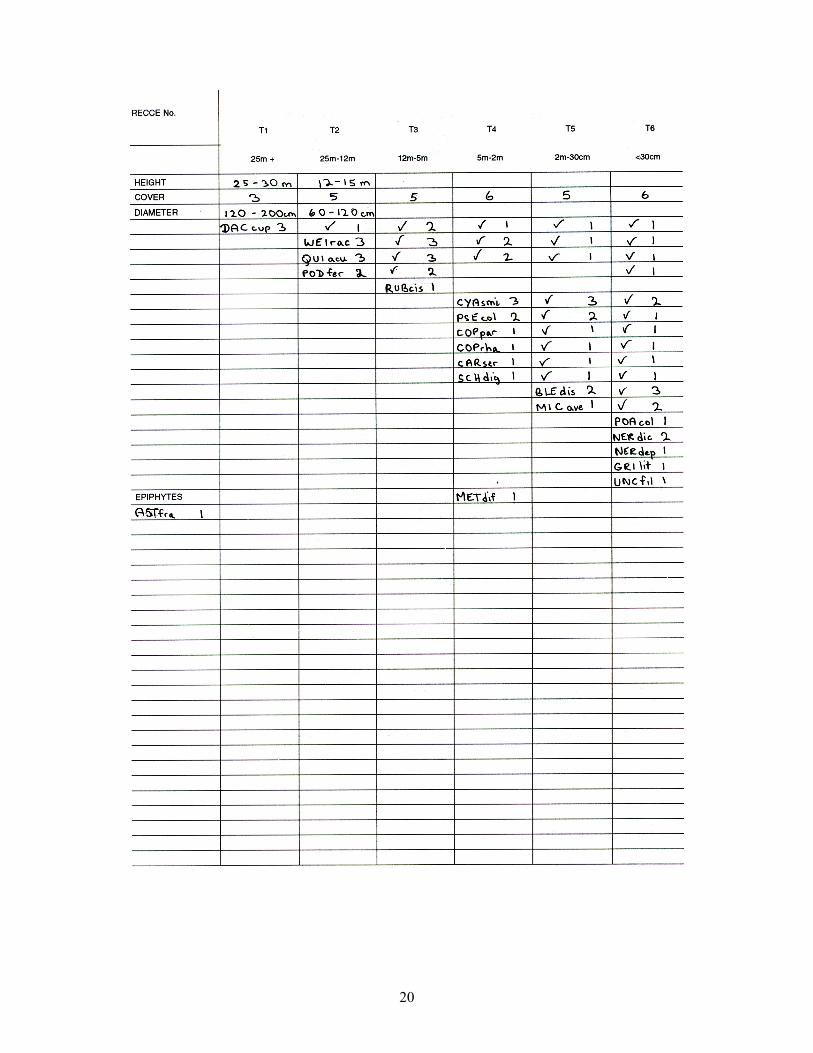
Full Recce description identification is recorded on the top left section of the Reconnaissance (Recce) Description Sheet, as shown in the Recce description of a hypothetical stand in Appendix 1.

• Recce description number: Record description number as an identifier, including transect line number when appropriate, in the space provided.

10

• Inventory: Record the name of the inventory, e.g., Hokitika Survey.

• Catchment: Record the name of the catchment in which the description is located, e.g., Whitcombe River.

• Subcatchment: If the description is located in a river or creek running into the main catchment, record as a subcatchment, e.g., Vincent Creek.

• Area: Describe the approximate location of the description.

• Aerial photo number: Record aerial photograph series and number on which the description occurs (if available).

• Date: Record day/month/year.

• Measured by: Record name of person doing description.

• Recorded by: Record name of person recording description data.

• Location diagram: In the space provided on the description sheet draw a quick sketch showing location of Recce description, including transect line when appropriate, and any prominent landscape features, e.g., small slips, gullies, banks.

• Map coordinates: These coordinates should be recorded after the field work is completed. For each description determine a grid reference using the NZMS Series 260 (metric) topographical map. Use the method described on all metric maps which will give a six-number grid reference. Every map sheet has a code, e.g., T16, L1, which should be recorded in front of the six-number grid reference. Zero is used as a place holder so that a code always uses four characters (S7 will become S007). The map coordinate can be recorded in the ‘Notes’ section. The New Zealand Mapping Grid (inch to the mile) has been used for much of the earlier data.

4.2 SITE CHARACTERISTICS

The main site characteristics that may relate to the type of vegetation in the area are also recorded on the Recce Description Sheet.

• Altitude: Measure to the nearest 10 m. Barometric altimeters should be corrected from spot heights on the topographical map each morning before work starts.

• Aspect: Measure at right angles to the general lie of the description area, with a compass to the nearest 5º.

• Slope: Measure the average slop of the area with an Abney level or hypsometer. Sight the Abney on an object at eye level some distance up or down the slope. The slope shape should be described as convex, concave, or linear.

11

• Physiography: Describe using four categories – ridge (including spurs), face, gully, or terrace. These categories can be used in combination with the slope shape to define a topographic position.

More detailed landform classifications can be used in addition to the standard methodology for studies focusing on relationships between compositional variation and landform. Dalrymple et al. (1968) developed a general nine-unit land surface model that has been used with Recce descriptions, and several other classifications have been used in publications using Recce description data (e.g., Myers et al. 1987; Rose et al. 1988; Whitehouse et al. 1990).

• Parent material: Usually read from geological survey maps. Any disagreement with

the broad map classification should be noted; this will be particularly important where there are extrusive/intrusive rocks.

• Soil depth: Measure the depth of the soil with a probe. Five measurements should be taken – one at description centre, one half-way to the description boundary above and below the description centre, and one half-way to the description boundary on either side of the description centre, along the slope contour. If the probe hits tree roots, the position should be changed slightly. The probe should be inserted at right angles to the slope. Measurements should be to the nearest 5 cm. Any depth over 50 cm is recorded as 50+.

A useful addition when compositional variation is being related to soil properties is to collect soil samples from the upper 10 cm of mineral soil. Soil samples analysed for chemical (pH, cations, percent base saturation) and physical properties (texture, water potential) are useful in the analysis and interpretation of compositional patterns, although this has not often been done in conjunction with Recce description data (e.g., Rose et al. 1988).

• Surface characteristics: Rock on surface – presence or absence of surface rock. Bedrock on surface – determine whether the surface rock is exposed bedrock or not. Quantity – percentage of exposed broken rock and percentage of soil at ground surface. Size – size of loose rock (if any) recorded as greater or less than 30 cm. Description – if possible classify loose rock into moraine (glacial deposits) or talus (erosion debris).

• Drainage: This parameter refers to the speed of runoff (slop) and degree of accumulation (internal drainage). Record as good, medium, or poor. Pakihi sites where water stands for long periods would be noted as poor drainage. On medium sites, runoff would be slow and water would accumulate in hollows for a day or two after rain. Good drainage would involve fast runoff and little accumulation of water.

It must be recognised that additions to the standard drainage method will not overcome the limitation that any subjective point-in-time assessment of soil drainage is difficult to use

12

consistently in other than extremes of soil drainage. However, several more refined soil drainage scales are available (e.g., Taylor & Pohlen 19762). 4.3 VEGETATION PARAMETERS

Vegetation parameters are visually assessed for rapid data collection. Interpretation of the data should be cautious and aimed at demonstrating large differences.

• Ground cover: Estimate the proportion of intercepts below 1.35 m height above ground level to the nearest 5% in the following classes:

V = live vascular vegetation including tree trunks and exposed roots M = non-vascular vegetation L = litter including dead logs, branches B = exposed soil (not covered by litter, vegetation, moss, or rocks) R = exposed rock on surface, either loose rock or bedrock

These will commonly add up to greater than 100%. Past Recce descriptions have often used the top intercept only, so that the sum of cover in all classes was 100%.

• Mean top height: Estimate the average height of the dominant canopy species, to

within 5%, and record in decimetres. Observer accuracy should be checked regularly by actual measurement.

• Canopy percentage: Estimate visually to the nearest 10% the proportion of sky blocked out by vegetation. This estimate is taken at the centre of the description at a height of 1.35 m (i.e., for vegetation less than 1.35 m record as 0).

• Basal area: Although basal area is not estimated on standard Recce descriptions, basal area can be determined in open forest stands from angle counts (Goulding 1986). With angle-count sampling, trees are included if the angle its diameter subtends at the plot centre is greater than the angle gauge specific critical angle. The contribution of each tree included is determined from a basal area factor, which is also specific to the instrument being used.

4.4 INCIDENTAL INFORMATION

The first two features are noted to provide the person who will ultimately interpret the data with an impression of what the area looks like.

• Approach: For the area adjacent to the Recce description describe the vegetation and physiography, taking particular notice of unusual species combinations. Records should be made of wind or snow damage, erosion, insect damage, fire history, and other influences.

13

• Notes: For the description area record phenology, insect damage, erosion, wind or snow damage, percentage of the ground surface permanently covered in water, fire history, mortality, and any other pertinent observations and impressions.

• Browsing: Record the degree of damage to all plant species, together with the animal responsible, i.e., light, medium, or heavy, by deer, brushtail possum, thar, chamois, insects, rabbits, and hares. State if unknown.

Light – browsing on one or two shoots only, on few plants. Medium – browsing on more than one or two shoots, but most not browsed. Heavy – browsing on most accessible shoots on most plants.

Browsed species should be recorded by abbreviations of the generic and specific names. The first three letters of the genus are recorded in capitals and the first three letters of the species in small letters, e.g., Metrosideros umbellata (southern rātā) becomes MET umb (Hall 1992). In the ‘Notes’ section, general features of browsing in the area can be described, e.g., bark stripping and the height of browsing. When compositional variation is specifically being related to the distribution and abundance of introduced browsing animals (e.g., Wardle et al. 1971), it is useful to record additional data on animal distribution and abundance (see Baddeley 1985).

• Birds: Record only positive identification by sighting or sound. Any distinctive bird sign should be noted.

When compositional variation is specifically being related to the distribution and abundance of birds it is useful to record additional bird observations using a recommended method (e.g. Dawson 1981). When compositional variation is specifically being related to habitat use by birds, Spurr & Warburton (1991) suggest that in addition to the standard height-tier information on top height of individual species should be noted.

• Cultural: Note any human interference, e.g., logged, burnt, tracked, cleared, mined, grazed (domestic stock), none.

4.5 HEIGHT-TIER INFORMATION

The vegetation is described in six height tiers with estimates of cover and stature. When a species is unknown, collect a specimen with as much of the vegetative and floral parts as practical. Record the species with a provisional name that reflects a feature of the plant. The specimen can be carefully stored for a day in a plastic bag. If it is to be stored for longer, it should be pressed in dry paper. The name given to the species must be included on a label with the sample for later identification.

14

On the reverse side of the Recce Description Sheet are six columns headed for each of the tier classes, and a seventh column for epiphytes. Allocate one species per row so that if the species occurs in other tiers it can be ticked on the same row, avoiding repetitive recordings (see Appendix 1). Care should be taken to ensure that recordings are made in the correct tier. This is especially important in T4, T5, and T6 if determining the impact of ungulate browsing is an objective, since it is the presence or absence of species in these tiers that indicates past and present usage and damage by ungulates.

• Tier One (T1): Record canopy trees taller than 25 m in this tier. Estimate their height range in metres and their diameter range at breast height over bark in centimetres (e.g., 28–30 m high, 60–100 cm in d.b.h.). Breast height is taken as 1.35 m above ground level at the side of the tree rather than the uphill or downhill position. Estimate and record the total foliage cover of all species in the tier (see below for cover classes).

• Tier Two (T2): Record species between 12–25 m tall. Estimate the height and diameter ranges and record them in the space provided. Estimate the total cover of all species in the tier.

• Tier Three (T3): Record species 5–12 m tall. In forest some of the understorey small-tree species, large shrubs, and tree ferns occur in this tier. If the canopy occurs in this height tier, record as for T2. Estimate the total cover of all species in the tier.

• Tier Four (T4): Record species 2–5 m tall. Estimate the total cover of all species in the tier.

• Tier Five (T5): Record all species 30 cm – 2 m tall. Estimate the total cover of all species in the tier.

• Tier Six (T6): Record all vascular plants up to 30 cm tall in this tier. Estimate the total cover of all species in the tier.

Cover classes modified from the Braun-Blanquet cover-abundance scale (see Mueller-Dombois & Ellenberg 1974) are also assigned to each species listed in each tier. The percentage foliage cover is visually estimated and recorded in one of six cover classes:

Percentage Cover

Cover Class Recordec

< 1 1–5 6–25 26–50 51–75 76–100

1 2 3 4 5 6

15

Several other similar cover-abundance scales exist (see Mueller-Dombois & Ellenberg 1974), of which that of Bailey & Poulton (e.g., Leathwick 1987) and Braun-Blanquet (e.g., Allen et al. 1991) have been applied to Recce description data. Note that both these can be condensed to the standard method.

• Epiphytes: Record species in column on left-hand side of plot sheet.

• Lianes and tree ferns: Record in the tier in which they occur. For instance, if the foliage of Rubus cissoides reaches 10 m above the ground, it wold be recorded in T3 (5–12 m).

The previous manual had different definitions for T1 and T2. For consistency these two tiers now also have fixed heights, which adds better structural information for tall forest. It is envisaged these tiers could be combined for analyses if data have been collected by both methods. In short vegetation the lower tiers can be subdivided for better structural information. For example, Rose (1985a) split T3 (30 cm – 2 m tier) into a 30 cm – 1 m tier and a 1 m – 2 m tier. Similarly the <30 cm tier could be subdivided in fellfield vegetation. Note that such divisions can be combined into the tiers used by the standard method for analyses with other data collected in the standard way. 5. DATA STORAGE

Systematic storage of the various forms of data collected is important. It may be many years before the data are looked at again, very likely by a different group of people. Documentation of datasets should include sample design, Recce description locations, and any departures from the standard method. It would be useful to lodge a copy of any data on the NIVS database held by FRI, Christchurch. 5.1 RECCE DESCRIPTION SHEETS

Recce description sheets are stored in ring-binder folders. The description sheets fit into an A4-sized folder. Description sheets are stored together in ascending order by Recce description number. The area and year of survey are written on the folder back. The sheets are also microfilmed and stored in a fireproof room for extra security. 5.2 MAPS AND AERIAL PHOTOGRAPHS

Maps containing Recce description locations can be stored in a map cabinet. Each map is fitted with a file mount and hung in the cabinet. Maps for one survey area are grouped and have the survey area recorded on the map mount.

16

Aerial photographs are stored in a filing cabinet, with all the photographs for one survey grouped together. 6. ACKNOWLDEGEMENTS

Many staff of the Forest Research Institute have been involved with developing the methodologies outlined in this manual, particularly Larry Burrows, Graeme Hall, John Leathwick, Kevin Platt, Alan Rose, Glenn Stewart, and John Wardle. This work was partially funded by the Department of Conservation and the Ministry for Research, Science, and Technology. 7. REFERENCES

ALLEN, R.B.; McLENNAN, M.J. 1983: Indigenous forest survey manual: Two inventory methods. Forest Research Institute, New Zealand, FRI Bulletin No. 48. 73 p.

ALLEN, R.B.; PEET, R.K. 1990: Gradient analysis of forests of the Sangre de Cristo Range, Colorado. Canadian Journal of Botany 68: 193–201.

ALLEN, R.B.; REIF, A.; HALL, G.M.J. 1991: Elevation distribution of conifer-broadleaved hardwood forests on South Island, New Zealand. Journal of Vegetation Science 2: 323–330.

AUSTIN, M.P. 1985: Continuum concept, ordination methods, and niche theory. Annual Review of Ecology and Systematics 16: 3961.

BADDELEY, C. 1985: Assessment of animal abundance. New Zealand Forest Service, FRI Bulledin No. 106. 44 p.

DALRYMPLE, J.B.; BLONG, R.J.; CONACHER, A.J. 1968: An hypothetical nine-unit landsurface model. Zeitschrift für Geomorphologie 12: 60–76.

DAWSON, D.G. 1981: Counting birds for a relative measure (index) of density. Pp. 12–16 in C.J. Ralph; J.M. Scott (eds), Estimating numbers of terrestrial birds. Studies in Avian Biology No.6.

ESPIE, P.R.; HUNT, J.E.; BUTTS, C.A.; COOPER, P.J.; HARRINGTON, W.M.A. 1984: Mackenzie Ecological Region; New Zealand Protected Natural Areas Programme. Department of Lands and Survey, Wellington.

FOREST RESEARCH INSTITUTE 1989: Databases for New Zealand’s indigenous vegetation. What’s New in Forest Research No. 175. 4 p.

GAUCH, H.G. 1982: Multivariate analysis in community ecology. Cambridge University Press, New York. 298 p.

GOULDING, C.J. 1986: Forest Inventory. Pp. 81–82 in Levack, H. (ed), Forestry Handbook. New Zealand Institute of Foresters, Wellington.

17

HAVEL, J.J. 1980: Application of fundamental synecological knowledge to practical problems in forest management, I : Theory and methods. Forest Ecology and Management 3: 1–29.

HALL, G.M. 1992: PC-RECCE Vegetation inventory data analysis. Ministry of Forestry, FRI Bulletin No. 177. 108 p.

HOLLOWAY, J.T. 1956: The National Forest Survey and the watershed protection forests. New Zealand Journal of Forestry 7(3): 61–67.

JONGMAN, R.H.G.; TER BRAAK, C.J.F.; VAN TONGEREN, O.F.R. 1987: Data analysis in community and landscape ecology. Pudoc, Wageningen.

KELLY, G.C.; PARK, G.N. 1986: The New Zealand Protected Natural Areas Programme: a scientific focus. New Zealand Biological Resources Centre Publication No.4. Department of Scientific and Industrial Research.

LEATHWICK, J.R. 1987: Waipapa Ecological Area: a study of vegetation pattern in a scientific reserve. Ministry of Forestry, FRI Bulletin No. 130. 82 p.

MANSON, B.R.; GUEST, R. 1975: Protection forests of the Wairau catchment. New Zealand Journal of Forestry Science 5(2): 123–142.

MUELLER-DOMBOIS, D.; ELLENBERG, H. 1974: Aims and Methods of Vegetation Ecology. John Wiley and Sons, New York. 547 p.

MYERS, S.C.; PARK, G.N.; OVERMARS, F.B. 1987: The New Zealand Protected Natural Areas Programme: A guidebook for the rapid ecological survey of natural areas. New Zealand Biological Resources Centre Publication No.6. New Zealand Department of Conservation, Wellington.

NEWSOME, P.F.J. 1987: The vegetative cover of New Zealand. Water and Soil Miscellaneous Publication 112, Wellington. 153 p.

NORTON, D.A.; LEATHWICK, J.R. 1990: The lowland vegetation patterns, south Westland, New Zealand 1. Saltwater Ecological Area. New Zealand Journal of Botany 28: 41–51.

ØKLAND, R.H. 1990: Vegetation ecology : theory, methods, and applications with reference to Fennoscandia. Sommerfeltia Supplement 1: 1–223.

REIF, A.; ALLEN, R.B. 1988: Plant communities of the steepland conifer-broadleaved hardwood forests of central Westland, South Island, New Zealand. Phytocoenologia 16: 145–224.

ROSE, A.B. 1985a: The high altitude grasslands. Pp. 110–124 in Davis, M.R.; Orwin, J. (eds), Report on a survey of the proposed wapiti area, West Nelson. New Zealand Forest Service, FRI Bulletin No. 84. 245 p.

ROSE, A.B. 1985b: The forests. Pp. 68–109 in Davis, M.R.; Orwin, J. (eds), Report on a survey of the proposed wapiti area, West Nelson. New Zealand Forest Service, FRI Bulletin No. 84. 245 p.

18

ROSE, A.B.; HARRISON, J.B.J.; PLATT, K.H. 1988: Alpine tussockland communities and vegetation-landform-soil relationships, Wapiti Lake, Fiordland. New Zealand Journal of Botany 26: 525–540.

SPURR, E.B.; WARBURTON, B. 1991: Methods of measuring the proportions of plant species present in forest and their effects on estimates of bird preferences for plant species. New Zealand Journal of Ecology 15: 171–175.

STEWART, G.H.; HARRISON, J.B.J. 1987: Plant communities, landforms, and soils of a geomorphically active drainage basin, Southern Alps, New Zealand. New Zealand Journal of Botany 25: 385–399.

STEWART, G.H.; ORWIN, J. (eds) 1986: Indigenous vegetation surveys : Methods and interpretation. Proceedings of a workshop, Forestry Research Centre, Forest Research Institute, Christchurch, May 1986. 67 p.

TAYLOR, N.H.; POHLEN, I.J. 1962: Soil survey method. Soil Bureau Bulletin No. 25. 242 p.

WARDLE, J.A.; HAYWARD, J. 1970: The forests and scrublands of the Taramakau and the effects of browsing by deer and chamois. Proceedings of the New Zealand Ecological Society 17: 80–91.

WARDLE, J.A.; HAYWARD, J.; HERBERT, J. 1971: Forests and scrublands of Northern Fiordland. New Zealand Journal of Forestry Science 1: 80–115.

WARDLE, J.A. 1974: Influence of introduced animals on the forests and scrublands of the Grey River headwaters. New Zealand Journal of Forestry Science 4: 459–486.

WHITEHOUSE, I.E.; BASHER, L.R.; TONKIN, P.J. 1990: A landform classification for PNA surveys in eastern Southern Alps. Land Resources Technical Record 19, Department of Scientific and Industrial Research, Lower Hutt.

WILLIAMS, P.A.; COURTNEY, S.; GLENNY, D.; HALL, G.M.J.; MEW, C. 1990: Pakihi and surrounding vegetation in North Westland, South Island. Journal of the Royal Society of New Zealand 20: 179–203.

19

APPENDIX 1 : Reconnaissance (Recce) Description Sheet

20

21

APPENDIX 2 : Equipment List This list specifies the equipment needed for a Recce description. Spares should be carried in case of loss or breakage.

Topographical map Aerial photograph Pen, pencil, and eraser Description sheet Altimeter Compass Abney level Angle gauge Soil probe Plastic bags (for plant material) Labels