NASA-CR-197950 i- J° Research Institute for Advanced Computer Science NASA Ames Research Center Recent Advances in Lanczos-based Iterative Methods for Nonsymmetric Linear Systems Roland W. Freund, Gene H. Golub, and No61 M. Nachtigal (NASA-CR-197950) RECENT ADVANCES IN LANCZQS-BASEO ITERATIVE METHOOS FOR NONSYMMETRIC LINEAR SYSTEMS (Research Inst. for Advanced Computer Science) 20 p G]I6_ N95-23611 Unclas 0043877 RIACS Technical Report 92.02 January 1992 To appear in Algorithmic Trends for Computational Fluid Dynamics in the 90's https://ntrs.nasa.gov/search.jsp?R=19950017191 2018-07-17T17:21:01+00:00Z
Transcript
NASA-CR-197950
i- J°Research Institute for Advanced Computer Science
NASA Ames Research Center
Recent Advances inLanczos-based Iterative Methods
for Nonsymmetric Linear Systems
Roland W. Freund, Gene H. Golub,
and No61 M. Nachtigal
(NASA-CR-197950) RECENT ADVANCESIN LANCZQS-BASEO ITERATIVE METHOOSFOR NONSYMMETRIC LINEAR SYSTEMS(Research Inst. for AdvancedComputer Science) 20 p
G]I6_
N95-23611
Unclas
0043877
RIACS Technical Report 92.02
January 1992
To appear in
Algorithmic Trends for Computational Fluid Dynamics in the 90's
Abstract. In recent years, there has been a true revival of the nonsymmetric Lanczos method. On
the one hand, the possible breakdowns in the classical algorithm are now better understood, and so-
called look-ahead variants of the Lanczos process have been developed, which remedy this problem.
On the other hand, various new Lanczos-based iterative schemes for solving nonsymmetric linear
systems have been proposed. This paper gives a survey of some of these recent developments.
1 Introduction
Many numerical computations involve the solution of large nonsingular systems of linear equations
Az = b. (1.1)
For example, such systems arise from finite difference or finite element approximations to partial
differential equations (PDEs), as intermediate steps in computing the solution of nonlinear prob-
lems, or as subproblems in large-scale l]near and nonlinear programming. Typically, the coefficient
"The work of these authors was supported by Cooperative Agreement NCC 2-387 between NASA and the Uni-
versities Space Research Association (USRA).
tThe work of this author wa_ supported in part by the National Science Foundation under Grant NSF CCR-
8821078,
2 R.W. Freund, G.B. Golub, and N.M. Nachtigal
matrix A of (1.1) is sparse and highly structured. A natural way to exploit the sparsity of A in the
solution process is to use iterative techniques, which involve A only in the form of matrLx-vector
products. Most iterative schemes of this type fall into the category of Krylov subspace methods:
they produce approximations x,_ to A-lb of the form
z,_ E x 0 ÷ K,,(r0, A), n = 1, 2, .... (1.2)
Here x 0 is any initial guess for A-lb, r 0 := b - Az o is the corresponding residual vector, and
K,_(r0, A ) := span{r0, Ar0,...,An-lr0} (1.3)
is the nth Krylov subspace generated by r 0 and A.
The most powerful iterative method of this type is the conjugate gradient algorithm (CG) due
to Hestenes and Stiefel [33], which is a scheme for linear systems (1.1) with Hermitian positive
definite A. Although CG was introduced as early as 1952, its true potential was not appreciated
until the 1970s. In 1971, Reid [45] revived interest in the method when he demonstrated its
usefulness for solving linear systems arising from self-adjoint elliptic PDEs. Moreover, it was realized
(see, e.g., [7]) that the performance of CG can be enhanced by combining it with preconditioning,
and efficient preconditioners, such as the incomplete Cholesky factorization [40], were developed.
Thereafter, the success of CG triggered an extensive search for CG-type Krylov subspace meth-
ods for non-Hermitian linear systems, and a number of such algorithms have been proposed; we
refer the reader to [1, 51, 48, 47, 17] and the references given there. Among the many properties
of CG, the following two are the most important ones: its nth iterate is defined by a minimization
property over Kn(ro, A), and the algorithm is based on three-term vector recurrences. Ideally, aCG-like method for non-Hermitian matrices would have features similar to these two. It would
produce iterates z,, in (1.2) that:
(i) are characterized by a minimization property over K,_(r0, A), such as the minimal residual
property
lib- Az,_[[ = min lib- Az[[, z,_ e Zo + g_(ro, A);zEzo+Kn(ro,A)
(ii) can be computed with little work per iteration and low overall storage requirements.
Unfortunately, it turns out that, for general non-Hermitian matrices, one cannot fulfill (i) and (ii)
simultaneously. This result is due to Faber and Manteuffel [10, 11] who have shown that, except
for a few anomalies, CG-type algorithms with (i) and (ii) exist only for matrices of the special form
A = e_e(T + aI), where T=T H, 8 E R, a E C, (1.4)
(see also Voevodin [55] and Joubert and Young [35]). Note that the class (1.4) consists of just theshifted and rotated Hermitian matrices. We remark that the important subclass of real nonsym-
metric matrices
A=I-S, where 3'=-S T is real, (1.5)
is contained in (1.4), with e_° = i, a = -i, and T = iS. Concus and Golub [6] and Widlund [56]
were the first to devise a CG-type algorithm for the family (1.5).
Most of the non-Hermitian Krylov subspace methods that have been proposed satisfy either
(i) or (ii). Until recently, the emphasis was on requirement (i), and numerous algorithms with
Advances in Lanczos-based Methods for Linear Systems 3
iteratescharacterizedby (i)or a similarconditionhave been developed,startingwith Vinsome's
Orthomin [54].The most widely used method in thisclassis the generalizedminimal residual
algorithm (GMRES) due to Saad and Schultz[49].Of course,none of thesemethods fulfills(ii),
and indeed,forallthesealgorithmswork per iterationand overallstoragerequirementsgrow linearly
with the iterationnumber n. Consequently,in practiceone cannot affordto run the fullversion
of these algorithms,and itisnecessaryto use restarts.For diffficultproblems,thisoftenresultsin
very slow convergence.
The second category of CG-like non-Hermitian Krylov subspace methods consistsof schemes
that satisfy (ii), but not (i). The archetype in this class is the classical biconjugate gradient algorithm
(BCG), which was proposed by Lanczos [38] already in 1952 and later revived by Fletcher [12] in
1976. Since no minimization condition of type (i) holds for BCG, the algorithm can exhibit--and
typically does--a rather irregular convergence behavior with wild oscillations in the residual norm.
Even worse, breakdowns in the form of division by 0 may be encountered during the iteration
process. In finite precision arithmetic, such exact breakdowns are very unlikely; however, near-
breakdowns may occur, leading to numerical instabilities in subsequent iterations.
The BCG method is intimately connected with the nonsymmetric Lanczos process [37] for
tridiagonalizing square matrices. In particular, the Lanczos algorithm in its original form is also
susceptible to breakdowns and potential numerical instabilities. In recent years, there has been
a true revival of the nonsymmetric Lanczos process. On the one hand, the possible breakdowns
in the classical algorithm are now better understood, and so-called look-ahead variants of the
Lanczos process have been developed, which remedy this problem. On the other hand, various new
Lanczos-based Krylov subspace methods for solving general non-Hermitian linear systems have
been proposed. Here we review some of these recent developments.
The remainder of the paper is organized as follows. In Section 2, we focus on the nonsymmetric
Lanczos process; in particular, we sketch a look-ahead variant of the method and briefly discuss
related work. We then turn to Lanczos-based Krylov subspace algorithms for non-Hermitian linear
systems. First, in Section 3, we consider the recently proposed quasi-minimal residual method
(QMI{.) and outline two implementations. In addition to matrix-vector products with the coefficient
matrix A of (1.1), BCG and QMR also require multiplications with its transpose A T. This is a
disadvantage for certain applications where A T is not readily available. It is possible to devise
Lanczos-based methods that do not involve A T, and in Section 4, we survey some of these so-called
transpose-free schemes. In Section 5, we make some concluding remarks.
Throughout the paper, all vectors and matrices are allowed to have real or complex entries.
As usual, M T and M H denote the transpose and conjugate transpose of a matrix M, respectively.
The vector norm ]lzl] = _ is always the Euclidean norm. The notation
= {¢(A) - a0 + alA +... + Ia0,...,a, e C}
is used for the set of all complex polynomials of degree at most n. Finally, A is always assumed to
be a square matrix of order N.
2 The Nonsymmetric Lanczos Process
In this section, we consider the nonsymmetric Lanczos process. Here the matrix A is not required
to be nonsingular.
4 R.W.Freund,G.H. Golub, and N.M. Nachtigal
2.1 A Look-Ahead Lanczos Algorithm
The La_czos method in its original form as proposed by Lanczos [37] can break down prematurely.
Taylor [52] and Parlett, Taylor, and Liu [44]--with their look-ahead Lanczos algorithm--were thefirst to devise a variant of the classical process that skips over possible breakdowns. We use the term
look-ahead Lanczos method in a broader sense to denote any extension of the standard algorithm
that circumvents breakdowns. In this section, we sketch an implementation of a look-ahead Lanczos
algorithm that was recently developed by Freund, Gutknecht, and Nachtigal [18].Given two nonzero starting vectors v1 E CN and w 1 E CN, the look-ahead Lanczos process
generates two sequences of vectors {vj}jn__x and {wj)jn__x such that, for n = 1, 2,...,
span {v,, v2,..., v,} = K, (vl, A), (2.1)
span{w 1, w2,. •., wn} = Kn(w x, AT).
Here, K,_(vI,A ) and K,_(wl, A T) denote the nth Krylov subspace of C N generated by v1 and A,
and w 1 and A T, respectively (of. (1.3)). Moreover, the Lanczos vectors are constructed so that the
holds. Here, the matrices V (k) and W (k) contain the Lanczos vectors built during the kth look-ahead
step. More precisely,
V(k) = [v._ v._+l "'" v._.,_l],
W(k)=[w._ w._+l "'" w.,.,_l],k = 1,...,l- 1,
and
where
V( t)=[v., v.,+l "'" v.],
W(O=[w., w.,+a "'" w.],
1 = n 1 < n 2 < ... < n k < "" < nt < n < hi+ 1.
The first vectors vn_ and w_k in each block are called regular, and any remaining vectors are calledinner. Note that l = l(n) denotes the index of the last constructed regular vector. Furthermore, in
(2.2), the blocks D (k) are nonsingular for k = 1,...,l- 1, and D (t) is nonsingular if n = nt+ 1 - 1.
With these preliminaries, the look-ahead Lanczos algorithm can be sketched as follows.
Algorithm 2.1 (Sketch of the look-ahead Lanczos process)
O) Choose nonzero vectors Vl, w 1 E CN.
Set VO) = vx, W (x) = Wl, DO) = (W(1))Tv (1).
Seth 1 =l,l=l, vo=wo=O, Vo=Wo=O.
For n = 1,2,..., do :
1) Decide whether to construct vn+ 1 and wn+ 1 as regular or inner vectors
and go to 2) or 3), respectively.
Advances in Lanczos-based Methods for Linear Systems 5
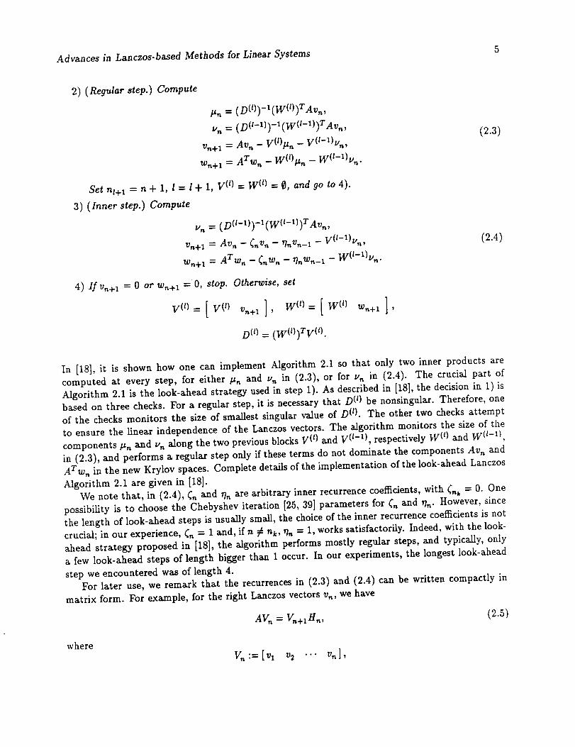
2) (Regular step.) Compute
It,, = (D(O)-x(W(O)T Avn,
Vn = (D(I-1))-I(W(I-1))TAvn,
Vn+_ = Avn - V(t)lZn - V(t-1)Vn,
Wn+ 1 = ATwn - W(l)l_n - W(t-1)vn.
Set nt+ 1 = n + l, l = l + l, V (t) = W (t) = O, and go to 4).
3) (Inner step.) Compute
u,, = (D(t-1))-I(W(t-x))T Av,,,
Vn+l = Avn - _,_Vn -- rl,aVn--1 -- V(t-1)Vn,
Wn+l = Arwn - f,,Wn - rlnWn__ - W(t-1)Vn •
4) If v,,+l = 0 or w,,+l = O, stop. Otherwise, set
V(') = [V(') Vn+, ], W(')= [W(" w,.,+x ],
D(O = (W(O)TV(O.
(2.3)
(2.4)
In [18], it is shown how one can implement Algorithm 2.1 so that only two inner products are
computed at every step, for either ttn and vn in (2.3), or for Vn in (2.4). The crucial part of
Algorithm 2.1 is the look-ahead strategy used in step 1). As described in [18], the decision in 1) is
based on three checks. For a regular step, it is necessary that D(l) be nonsingular. Therefore, one
of the checks monitors the size of smallest singular value of D (0. The other two checks attempt
to ensure the linear independence of the Lanczos vectors. The algorithm monitors the size of the
components ttn and v,_ along the two previous blocks V (t} and V (t-_}, respectively W(0 and W (t-l},
in (2.3), and performs rt regular step only if these terms do not dominate the components Av,_ and
ATw,_ in the new Krylov spaces. Complete details of the implementation of the look-ahead Lanczos
Algorithm 2.1 are given in [18].
We note that, in (2.4), _n and 0r are axbitrary inner recurrence coefficients, with _n, = 0. Onepossibility is to choose the Chebyshev iteration [25, 39] parameters for Q and r/,v However, since
the length of look-ahead steps is usually small, the choice of the inner recurrence coefficients is not
crucial; in our experience, Cn = 1 and, if n _ n_, On = 1, works satisfactorily. Indeed, with the look-
ahead strategy proposed in [18], the algorithm performs mostly regular steps, and typically, only
a few look-ahead steps of length bigger than 1 occur. In our experiments, the longest look-ahead
step we encountered was of length 4.
For later use, we remark that the recurrences in (2.3) and (2.4) can be written compactly in
matrix form. For example, for the right Lanczos vectors vn, we have
AVn= vn+ Hn, (2.5)
where
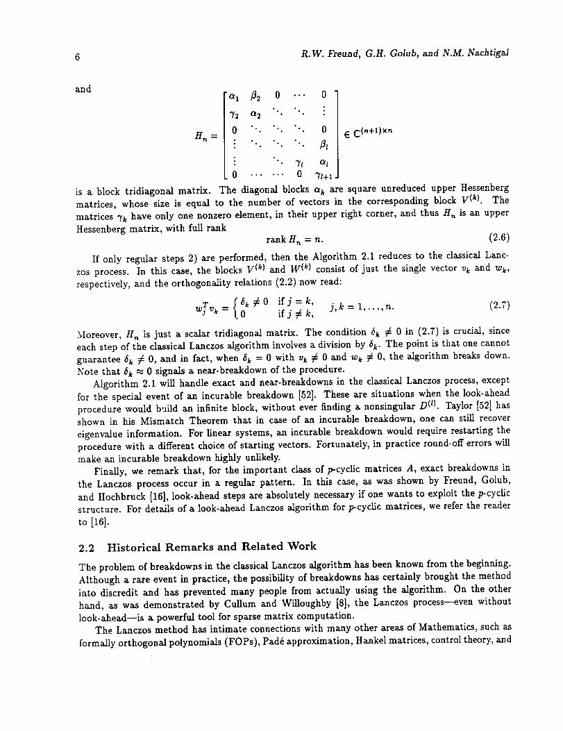
6 R.W.Freund, G.H. Golub, and N.M. Nachtigal
and'% d2 0 .-.
• •72 cw2 "
°.. °° *..
°,. °. "°
" 71
0 ...... 0
0
0E C (n+1)x'_
otI
is a block tridiagonal matrix. The diagonal blocks a k are square unreduced upper Hessenberg
matrices, whose size is equal to the number of vectors in the corresponding block V (k). The
matrices "rk have only one nonzero element, in their upper right corner, and thus H,_ is an upper
Hessenberg matrix, with full rank
rank H,_ = n. (2.6)
If only regular steps 2) axe performed, then the Algorithm 2.1 reduces to the classical Lanc-zos process. In this case, the blocks V (k) and W (k) consist of just the single vector % and wk,
respectively, and the orthogonality relations (2.2) now read:
{ _k_O .,n. (2.7)ifj=k,
wTvk= 0 ifj_k, j,k=l,..
Moreover, Hn is just a scalar tridiagonal matrix. The condition _k _ 0 in (2.7) is crucial, since
each step of the classical Lanczos algorithm involves a division by 5k- The point is that one cannot
guarantee 5k _ 0, and in fact, when 5k = 0 with vk y_ 0 and w_ y_ 0, the algorithm breaks down.
Note that 5k _ 0 signals a near-breakdown of the procedure.
Algorithm 2.1 will handle exact and near-breakdowns in the classical Lanczos process, except
for the special event of an incurable breakdown [52]. These are situations when the look-ahead
procedure would b,_ild an infinite block, without ever finding a nonsingular D (l). Taylor [52] has
shown in his Mismatch Theorem that in case of an incurable breakdown, one can still recover
eigenvalue information. For linear systems, an incurable breakdown would require restarting the
procedure with a different choice of starting vectors. Fortunately, in practice round-off errors will
make an incurable breakdown highly unlikely.
Finally, we remark that, for the important class of p-cyclic matrices A, exact breakdowns in
the Lanczos process occur in a regular pattern. In this case, as was shown by Freund, Golub,
and Hochbruck [16], look-ahead steps are absolutely necessary if one wants to exploit the p-cyclic
structure. For details of a look-ahead Lanczos algorithm for p-cyclic matrices, we refer the reader
to [16l.
2.2 Historical Remarks and Related Work
The problem of breakdowns in the classical Lanczos algorithm has been known from the beginning.
Although a rare event in practice, the possibility of breakdowns has certainly brought the method
into discredit and has prevented many people from actually using the algorithm. On the other
hand, as was demonstrated by Cullum and Willoughby [8], the Lanczos process--even without
look-ahead--is a powerful tool for sparse matrix computation.
The Lanczos method has intimate connections with many other areas of Mathematics, such as
formally orthogonal polynomials (FOPs), Padd approximation, Hankel matrices, control theory, and
Advances in Lanczos-based Methods for Linear Systems 7
coding theory. The problem of breakdowns has a correspondingformulationin allof these areas,
and remedies for breakdowns in these differentsettingshave been known for quite some time.
For example, the breakdown in the Lanczos processisequivalentto a breakdown of the generic
three-termrecurrencerelationfor FOPs, and itiswellknown how to overcome such breakdowns
by modifying the recursionsfor FOPs (see [26,9, 31] and the referencesgiven there). In the
context of the partialrealizationproblem in controltheory,remedies for breakdowns were given
in [36, 27]. The Lanczos process is also closely related to fast algorithms for the factorization of
Ha_kel matrices, and again it was known how to overcome possible breakdowns of these algorithms
(see [32, 22] and the references therein). However, in all these cases, only the problem of exactbreakdowns was addressed.
The look-ahead Lanczos algorithm of Taylor [52] and Parlett, Taylor, and Liu [44] was the first
procedure that remedies both exact and near-breakdowns. We point out that their implementation
is different from Algorithm 2.1. In particular, it always requires more work per step than Algo-
rithm 2.1, and it does not reduce to the classical Lanczos process in the absence of look-ahead
steps. Furthermore, in [52, 44], details axe given only for the case of look-ahead steps of size 2, and
their algorithm does not generalize easily to blocks of more than two vectors.
In recent years, there has been a revival of the nonsymmetric Lanczos algorithm, and since 1990,
in addition to the papers we have already cited in this section, there are several others dealing with
various aspects of the Lanczos process. We refer the reader to [2, 3, 4, 22, 29, 34, 43] and the
references given therein.
3 The Quasi-Minimal Residual Approach
We now return to linear systems (1.1). From now on, it is always assumed that the matrix A is
nonsingular. In this section, we describe the QMR method. The procedure was first proposed by
Freund [13, 15] for the case of complex symmetric matrices A = A T, and then extended by Freund
and Nachtigai [19] for the case of general non-Hermitian matrices.
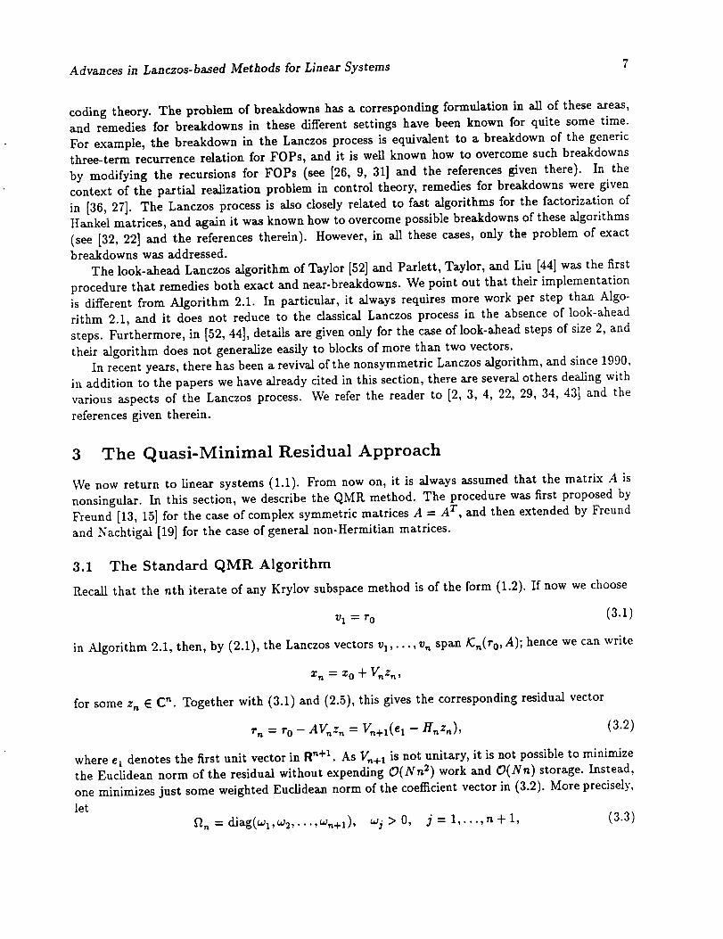
3.1 The Standard QMR Algorithm
Recall that the nth iterate of any Krylov subspace method is of the form (1.2). If now we choose
v 1 = r0 (3.1)
in Algorithm 2.I, then, by (2.1), the Lanczos vectors vl,..., v,, span/C,t(r0, A); hence we can write
xrL -- x 0 + V,tzrL,
for some z, E C'*. Together with (3.1) and (2.5), this gives the corresponding residual vector
r,_ = r0 - AV,_z n = Vr,+l(e _ - H,tz,t), (3.2)
where e 1 denotes the first unit vector in R '_+1. As V,t+l is not unitary, it is not possible to minimizethe Euclidean norm of the residual without expending O(Nn 2) work and O(Nn) storage. Instead,
one minimizes just some weighted Euclidean norm of the coefficient vector in (3.2). More precisely,let
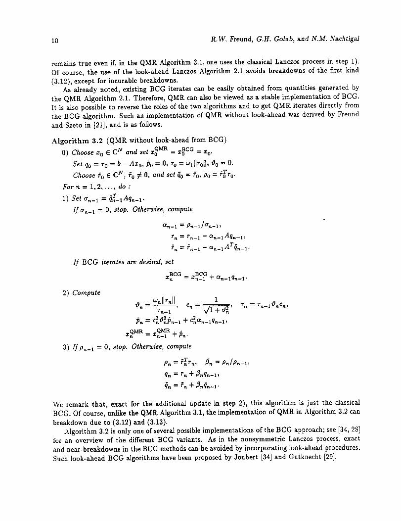
Choose ro E C N, ro 7t O, and set qo = to, Po = r0Tr0 •
For n = 1,2,..., do :
1) Set a,__ x = 4T_IAq,_I.
If a,,_ 1 = O, stop. Otherwise, compute
Otn_ 1 = Pn_l/(Tn_l,
r_ = rn_ 1 -- ¢_._lAq._l,
fa = fn-1 - an-lATqa-1 •
If BCG iterates are desired, set
zBCG = zBCGn n-I + an-lq--l"
2) Compute llr.II 1
7",_1 V/'_n '
Cn I_nPn_ 1 _- C20_n_lqn_l ,Pn -- 2 2 "
QMR X QMR Jr ]_nn -- n--1 "
3) If p,__, = O, stop. Otherwise, compute
p. = fTr., _,_= p./p._,,
q. = r. + $.q.-1,
r. = r._l_.C_,
We remark that, exact for the additional update in step 2), this algorithm is just the classical
BCG. Of course, unlike the QMR. Algorithm 3.1, the implementation of QMR. in Algorithm 3.2 can
breakdown due to (3.12) and (3.13).
Algorithm 3.2 is only one of several possible implementations of the BCG approach; see [34, 28]for an overview of the different BCG variants. As in the nonsymmetric Lanczos process, exact
and near-breakdowns in the BCG methods can be avoided by incorporating look-ahead procedures.
Such look-ahead BCG algorithms have been proposed by Joubert [34] and Gutknecht [29].
Advances in Lanczos-based Methods for Linear Systems 11
4 Transpose-Free Methods
Krylov subspace methods such as BCG and QMR, which are based directly on the Lanczos process,
involve matrix-vector products with A and A T. This is a disadvantage for certain applications,
where A T is not readily available. It is possible to devise Lanczos-based Krylov subspace methods
that do not involve the transpose of A. In this section, we give an overview of such transpose-free
schemes.
First, we consider the QMR algorithm. As pointed out by Freund and Zha [23], in principle
it is always possible to eliminate A T altogether, by choosing the starting vector w 1 suitably. This
observation is based on the fact that any square matrix is similar to its transpose• In particular,
there always exists a nonsingular matrix P such that
AT p = PA. (4.1)
Now suppose that in the QMR Algorithm 3.1 we choosethe special starting vector w1 = Pv I . Then,
with (4.1), one readily verifies that the vectors generated by look-ahead Lanczos Algorithm 2.1
satisfy
w,_ = Pv,_ for all n. (4.2)
Hence, instead of updating the left Lanczos vectors {w_} by means of the recursions in (2.3) or (2.4),
they can be computed directly from (4.2). The resulting QMlZ algorithm no longer involves the
transpose of A; in exchange, it requires one matrix-vector multiplication with P in each iteration
step. Therefore, this approach is only viable for special classes of matrices A, for which one can
find a matrix P satisfying (4.1) easily, and for which, at the same time, matrix-vector products
with P can be computed cheaply. The most trivial case are real or complex symmetric matrices
A = A T, which fulfill (4.1) with P = 1. Another simple case are Toeplitz matrices A, i.e., matrices
whose entries are constant along each diagonal. Toeplitz matrices satisfy (4.1) with P = J, where
J __ [i°i]• °° 1
° •
oo.
is the N x N antidiagonal identity matrix. Finally, the condition (4.1) is also fulfilled for matricesof the form
A = TM -1, P = M -1,
where T and M are real symmetric matrices and M is nonsingular. Matrices of this type arise when
real symmetric linear systems Tz = b are preconditioned by M. The resulting QMlZ algorithm for
the solution of preconditioned symmetric linear system has the same work and storage requirements
as preconditioned SYMMLQ or MINP_ES [42]. However, the QMR approach is more general, in
that it can be combined with any nonsingular symmetric preconditioner M, while SYMMLQ and
MINRES require M to be positive definite (see, e.g., [24]). For strongly indefinite matrices T, the
use of indefinite preconditioners M typically leads to considerably faster convergence; see [23] for
numerical examples.
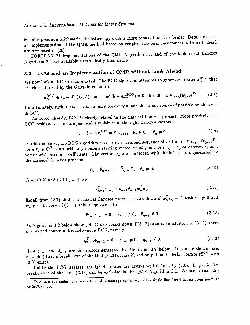
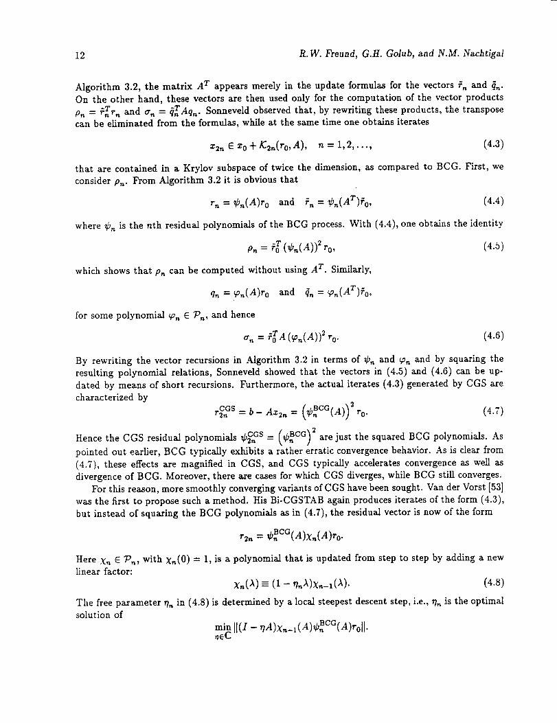
Next, we turn to transpose-free variants of the BCG method. Sonneveld [50] with his CGS
algorithm was the first to devise a transpose-free BCG-type scheme. Note that, in the BCG
12 R.W. Freund, G.H. Golub, and N.M. Nachtigal
Algorithm 3.2, the matrix A T appears merely in the update formulas for the vectors rn and {,.
On the other hand, these vectors are then used only for the computation of the vector products
p'* = _nrr'* and a,, - (trAq'*. Sonneveld observed that, by rewriting these products, the transposecan be eliminated from the formulas, while at the same time one obtains iterates
x2". E Zo + ]C2n(ro,A), n = 1,2,..., (4.3)
that are contained in a Krylov subspace of twice the dimension, as compared to BCG. First, we
consider p_. From Algorithm 3.2 it is obvious that
r n -- Cn(A)r0 and _, = _bn(Ar)_o, (4.4)
where _,_ is the nth residual polynomials of the BCG process. With (4.4), one obtains the identity
Pn = r0T (¢'*(A)) 2 r0, (4.5)
which shows that p,, can be computed without using A T. Similarly,
an = ¢Pn(A)ro and qn = _,_(AT)ro,
for some polynomial _,, E 7_,, and hence
an = fToA (¢2"*(A ) )2 ro • (4.6)
By rewriting the vector recursions in Algorithm 3.2 in terms of _b'*and _'* and by squaring the
resulting polynomial relations, Sonneveld showed that the vectors in (4.5) and (4.6) can be up-
dated by means of short recursions. Furthermore, the actual iterates (4.3) generated by CGS are
characterized by
rCGS ( ))22,, = b- Az2"* = ¢_CC(A ro. (4.7)
Hence the CGS residual polynomials !b2cnGs (¢BCG) 2= are just the squared BCG polynomials. As
pointed out earlier, BCG typically exhibits a rather erratic convergence behavior. As is clear from
(4.7), these effects are magnified in CGS, and CGS typically accelerates convergence as well as
divergence of BCG. Moreover, there axe cases for which CGS diverges, while BCG still converges.For this reason, more smoothly converging variants of CGS have been sought. Van der Vorst [53]
was the first to propose such a method. His Bi-CGSTAB again produces iterates of the form (4.3),
but instead of squaring the BCG polynomials as in (4.7), the residual vector is now of the form
r2n = o_CG(A)x'*(A)ro .
Here X'* E 7an, with X'*(O) = 1, is a polynomial that is updated from step to step by adding a newlinear factor:
X'*(A) - (I - rI'*A)X'*_:(A). (4.8)
The free parameter rl". in (4.8) is determined by a local steepest descent step, i.e., r/'* is the optimalsolution of
min II(I - rlA)x'*-:(A)_CC(A)roI[ •neC
Advances in Lanezos-based Methods for Linear Systems 13
Due to the steepestdescentsteps,Bi-CGSTAB typicallyhas much smoother convergencebehavior
than BCG or CGS. However, thenorms ofthe Bi-CGSTAB residualsmay stilloscillateconsiderably
for difficultproblems. Finally,Gutknecht [30]has noted that,for realA, the polynomialsXn will
always have realroots only,even ifA has complex eigenvalues.He proposed a variantof Bi-
CGSTAB with polynomials (4.8)thatare updated by quadraticfactorsin each stepand thus can
have complex rootsingeneral.
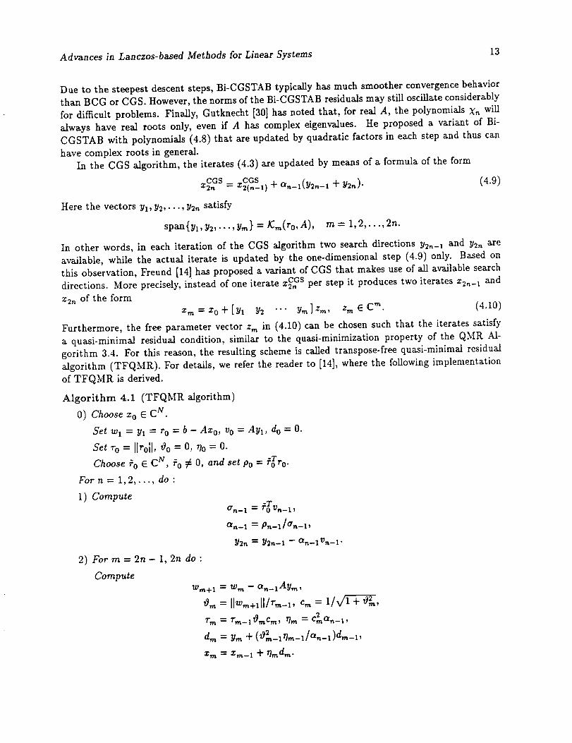
In the CGS algorithm,the iterates(4.3)are updated by means ofa formula ofthe form
:CGS _CGS2n - "_2(,-I) + an-1(Y2--1 + Y2,)" (4.9)
Here the vectors Yl, Y2,. -., Y2n satisfy
span{_,,y2,...,y,,) =/C,,(_o,A), m = 1,2,...,2n.
In other words, in each iteration of the CGS algorithm two search directions Y_,,-1 and Y2, are
available, while the actual iterate is updated by the one-dimensional step (4.9) only. Based on
this observation, Freund [14] has proposed a variant of CGS that makes use of all available search
directions. More precisely, instead of one iterate zCnGs per step it produces two iterates z2__ 1 and
z2n of the form
zm=Xo'F[Yl Y2 ... y,n]z,_, zm EC m. (4.10)
Furthermore, the free parameter vector zm in (4.10) can be chosen such that the iterates satisfy
a quasi-minimal residual condition, similar to the quasi-minimization property of the QMR Al-
gorithm 3.4. For this reason, the resulting scheme is called transpose-free quasi-minimal residual
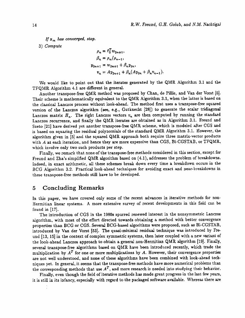
algorithm (TFQMR.). For details, we refer the reader to [14], where the following implementation
We would like to point out that the iterates generated by the QMP, Algorithm 3.1 and the
TFQMR. Algorithm 4.1 are different in general.
Another transpose-free QMR method was proposed by Chan, de Pillis, and Van der Vorst [5].
Their scheme is mathematically equivalent to the QMR Algorithm 3.1, when the latter is based on
the classical Lanczos process without look-ahead. The method first uses a transpose-free squared
version of the Lanczos algorithm (see, e.g., Gutknecht [28]) to generate the scalar tridiagonal
Lanczos matrix H,,. The right Lanczos vectors v,, are then computed by running the standard
Lanczos recurrence, and finally the QMR iterates are obtained as in Algorithm 3.1. Freund and
Szeto [21] have derived yet another transpose-free QMR scheme, which is modeled after CGS and
is based on squaring the residual polynomials of the standard QMR Algorithm 3.1. However, the
algorithm given in [5] and the squared QMR approach both require three matrix-vector productswith A at each iteration, and hence they are more expensive than CGS, Bi-CGSTAB, or TFQMR,
which involve only two such products per step.
Finally, we remark that none of the transpose-free methods considered in this section, except for
Freund and Zha's simplified QMR algorithm based on (4.1), addresses the problem of breakdowns.
Indeed, in exact arithmetic, all these schemes break down every time a breakdown occurs in the
BCG Algorithm 3.2. Practical look-ahead techniques for avoiding exact and near-breakdowns in
these transpose-free methods still have to be developed.
5 Concluding Remarks
In this paper, we have covered only some of the recent advances in iterative methods for non-
Hermitian linear systems. A more extensive survey of recent developments in this field can be
found in [17].The introduction of CGS in the 1980s spurred renewed interest in the nonsymmetric Lanczos
aigorithm, with most of the effort directed towards obtaining a method with better convergence
properties than BCG or CGS. Several BCG-based algorithms were proposed, such as Bi-CGSTAB,
introduced by Van der Vorst [53]. The quasi-minimal residual technique was introduced by Fre-
und [13, 15] in the context of complex symmetric systems, then later coupled with a new variant of
the look-ahead Lanczos approach to obtain a general non-Hermitian QMt_ algorithm [19]. Finally,
several transpose-free algorithms based on QMR have been introduced recently, which trade the
multiplication by A T for one or more multiplications by A. However, their convergence properties
are not well understood, and none of these algorithms have been combined with look-ahead tech-
niques yet. In general, it seems that the transpose-free methods have more numerical problems than
the corresponding methods that use A T , and more research is needed into studying their behavior.
Finally, even though the field of iterative methods has made great progress in the last few years,
it is still in its infancy, especially with regard to the packaged software available. Whereas there are
Advances in Lanczos-based Methods for Linear Systems 15
well-established robust general-purpose solvers based on direct methods, the same cannot be said
about solvers based on iterative methods. There are no established iterative packages of the same
robustness and wide acceptance as, for example, the LINPACK library, and as a result many of the
scientists who use iterative methods write their own specialized solvers. We feel that this situation
needs to change, and we would like to encourage researchers to provide code for their methods.
References
[1] O. Axelsson, Conjugate gradient type methods for unsymmetric and inconsistent systems of
Linear equations, Linear Algebra Appl. 29 (1980), pp. 1-16.
[2]D.L. Boley, S. Elhay, G.H. Golub, and M.H. Gutknecht, Nonsymmetric Lanczos and find-
ing orthogonal polynomials associated with indefinite weights, Numer. Algorithms 1 (1991),
pp. 21-43.
[3] D.L. Boley and G.H. Golub, The nonsymmetric Lanczos algorithm and controllability, Systems
Control Lett. 16 (1991), pp. 97-105.
[4] C. Brezinski, M. Redivo Zaglia, and H. Sadok, A breakdown-free Lanczos type algorithm for
solving linear systems, Technical Report ANO-239, Universit4 des Sciences et Techniques de
Lille Flandres-Artois, ViUeneuve d'Ascq, France, 1991.
Is] T.F. Chan, L. de PiUis, and H.A. Van der Vorst, A transpose-free squared Lanczos algo-
rithm and application to solving nonsymmetric linear systems, Technical Report CAM 91-17,
Department of Mathematics, University of California, Los Angeles, CA, 1991.
[6] P. Concus and G.H. Golub, A generalized conjugate gradient method for nonsymmetric systems
of linear equations, in Computing Methods in Applied Sciences and Engineering (R. Glowinski
and J.L. Lions, eds.), Lecture Notes in Economics and Mathematical Systems 134, Springer,
Berlin, 1976, pp. 56-65.
[7] P. Concus, G.H. Golub, and D.P. O'Leary, A generalized conjugate gradient method for the
numerical solution of elliptic partial differential equations, in Sparse Matriz Computations
(J.R. Bunch and D.J. Rose, eds.), Academic Press, New York, 1976, pp. 309-332.
[8] J. Cullum and R.A. Willoughby, A practical procedure for computing eigenvaiues of
large sparse nonsymmetric matrices, in Large Scale Eigenvalue Problems (J. CuUum and
R.A. Willoughby, eds.), North-Holland, Amsterdam, 1986, pp. 193-240.
[9] A. DratLx, Polyn6mes Orthogonauz Formels - Applications, Lecture Notes in Mathematics
974, Springer, Berlin, 1983.
[10] V. Faber and T. Manteuffel, Necessary and sufficient conditions for the e_stence of a conjugate
gradient method, SIAM J. Numer. Anal. 21 (1984), pp. 352-362.
[11] V. Faber and T. Manteuffel, Orthogonal error methods, SIAM J. Numer. Anal. 24 (1987),
pp. 170-187.
16 R.W. Freund, G.H. Golub, and N.M. Nachtigal
[12] R. Fletcher, Conjugate gradient methods for indefinite systems, in Numerical Analysis Dundee
1975 (G.A. Watson, ed.), Lecture Notes in Mathematics 506, Springer, Berlin, 1976, pp. 73-89.
[13] R.W. Freund, Conjugate gradienttype methods forlinearsystems with complex symmetric
coefficientmatrices,RIACS TechnicalReport 89.54,NASA Ames Research Center,Moffett
Field,CA, 1989.
[14]
[15]
[16]
R.W. Freund, A transpose-free quasi-minimal residual algorithm for non-Hermitian linear sys-
tems, RIACS Technical Report 91.18, NASA Ames Research Center, Moffett Field, CA, 1991.
R.W. Freund, Conjugate gradient-type methods for linear systems with complex symmetric
coefficient matrices, SIAM J. Sci. Stat. Comput. 13 (1992), to appear.
R.W. Freund, G.tt. Golub, and M. ttochbruck, Krylov subspace methods for non-Hermitian
p-cycllc matrices, Technical Report, RIACS, NASA Ames Research Center, Moffett Field, CA,1992.
[17] R.W. Freund, G.H. Golub, and N.M. Nachtigal, Iterative solution of linear systems, RIACS
Technical Report 91.21, NASA Ames Research Center, Moffett Field, 1991, to appear in ActaNumerica.
[18]
[19]
[2o]
R.W.
ahead
Ames
Freund, M.H. Gutknecht and N.M. Nachtigal (1991b), An implementation of the look-
Lanczos algorithm for non-Hermitian matrices, Technical Report 91.09, RIACS, NASA
Research Center, Moffett Field, CA, 1991, SIAM J. Sci. Stat. Comput., to appear.
R.W. Freund and N.M. Nachtigal, QMR: a quasi-minimal residual method for non-Hermitian
linear systems, Numer. Math. 60 (1991), pp. 315-339.
R.W. Freund, N.M. Nachtigal, and T. Szeto, An implementation of the QMR method based
on coupled two-term recurrences, Technical Report, RIACS, NASA Ames Research Center,
Moffett Field, CA, 1992.
[21] R.W. Freund and T. Szeto, A quasi-minimal residual squared algorithm for non-Hermitian
linear systems, Technical Report 91.26, RIACS, NASA Ames Research Center, Moffett Field,CA, 1991.
[22]
[23]
[24]
R.W. Freund and H. Zha, A look-ahead algorithm for the solution of general Hankel systems,
Technical Report 91.24, RIACS, NASA Ames Research Center, Moffett Field, CA, 1991.
R.W. Freund and H. Zha, Simplifications of the nonsymmetric Lanczos process and a new
algorithm for solving indefinite symmetric linear systems, Technical Report, RIACS, NASA
Ames Research Center, Moffett Field, CA, 1992.
P.E. Gill, W. Murray, D.B. Ponceledn, and M.A. Sannders, Preconditioners for indefinite
systems arising in optimization, Technical Report SOL 90-8, Stanford University, Stanford,CA, 1990.