Recent advances in numerical modelling of deep-stabilized soil

Minna Karstunen, University of Glasgow, ScotlandHarald Krenn, Donaldson Associates Ltd, Glasgow, Scotland

Asko Aalto, Helsinki University of Technology, Finland

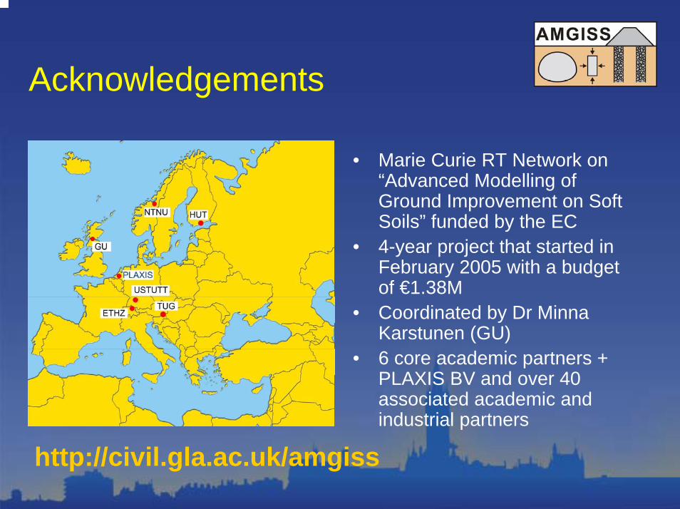
Acknowledgements

• Marie Curie RT Network on “Advanced Modelling of Ground Improvement on Soft Soils” funded by the EC

• 4-year project that started in February 2005 with a budget of €1.38M

• Coordinated by Dr Minna Karstunen (GU)

• 6 core academic partners + PLAXIS BV and over 40 associated academic and industrial partners

http://civil.gla.ac.uk/amgiss

Acknowledgements

• The experimental programme was funded by the Academy of Finland (Grant No 53936)

• The research programme on deep-stabilization was funded by TEKES (the National Technology Agency in Finland); deep-stabilization contractors: Rakennus Oy Lemminkäinen, YIT-Rakennus Oy and Rakentajat Piippo & Pakarinen Oy; the developers: City of Helsinki, City of Espoo, City of Vantaa, Finnish Road Enterprise, Finnish Rail Administration; the binder producers: Nordkalk Oy Ab, Finnsementti Oy and the consultancy: SCC Viatek Oy.

• The work by the second author was sponsored by Donaldson Associates Ltd and the Faculty of Engineering at the University of Glasgow.

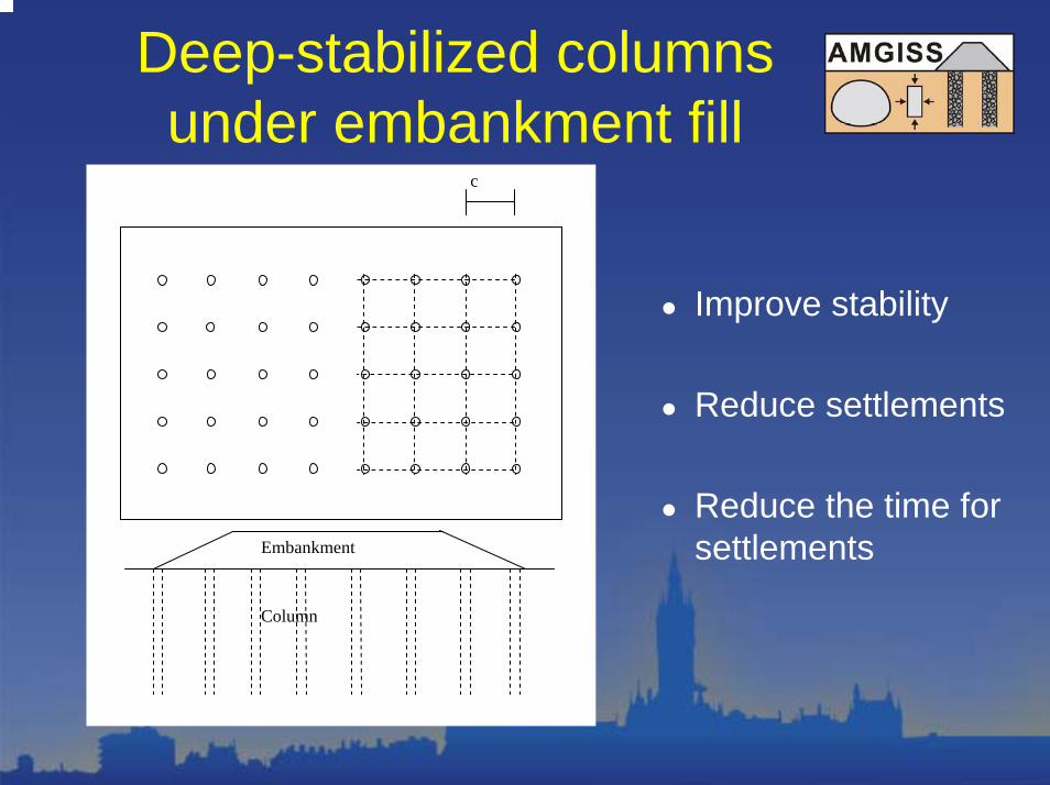
Deep-stabilized columnsunder embankment fill

c

Embankment

Column

Improve stability

Reduce settlements

Reduce the time for settlements

Why numerical modelling?

• Current design methods are simplistic and limited (based on work by Broms & Boman in 1970’s)

• Soft soils are very complex non-linear materials, exhibiting features such as anisotropy, bonding and creep

• Mechanics of in situ stabilized soils is complex and unfortunately (yet) not very well understood

• The problem has a complex 3D geometry

FE modelling

• Equilibrium, compatibility, stress-strain relationship and boundary conditions fulfilled

• Enables adapting “realistic” constitutive models for the materials (natural soil and stabilized soil)

• Possible to model realistically soil-structure interaction

• Now also possible to use 3D modelling• Numerical “benchmark” simulations and

parametric studies can be used as tools to develop design guidelines

Soft soil modelling

4 different constitutive models:• Modified Cam Clay (isotropic hardening model)• Soft-Soil-Creep model (MCC type of model that

comes as standard in PLAXIS), with creep set (effectively) to zero

• S-CLAY1 (accounts for initial and plastic-strain induced anisotropy)

• S-CLAY1S (accounts for anisotropy and bonding, and degradation of bonds)

S-CLAY1/S-CLAY1S

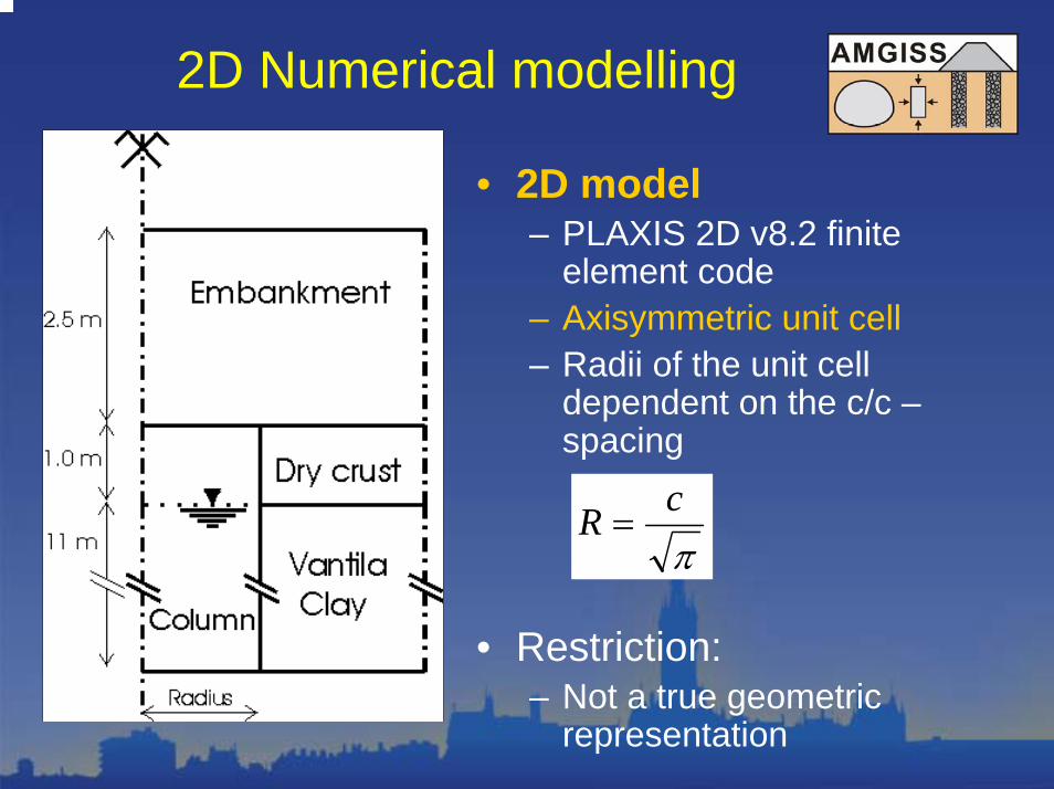
Idealised soil profile

Vanttila clay (Finland)– Dry crust (0-1m depth)

• over-consolidated (POP 30kPa)• Limited lab data available

– WT at 1 m depth– Soft Vanttila clay (1-12 m

depth)• Lightly over-consolidated (POP

10 kPa)• Plenty of lab data available

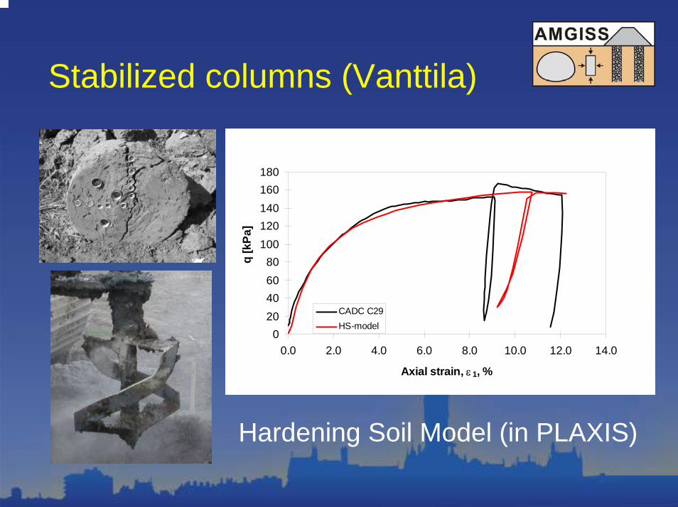
Stabilized columns (Vanttila)

020406080

100120140160180

0.0 2.0 4.0 6.0 8.0 10.0 12.0 14.0

Axial strain, ε 1, %

q [k

Pa]

CADC C29HS-model

Hardening Soil Model (in PLAXIS)

Soil parameters• Initial values for state parameters

• Conventional soil constants

• Additional soil constants for S-CLAY1 and S-CLAY1S

Soil Depth e0 POP [kPa] α xDry crust 0 - 1 1.7 30 0.63 90Vantilla clay 1 - 11 3.2 10 0.46 20

Soil γ[kN/m3]

κ ν’ λ M kx= ky[m/day]

Dry crust 13.8 0.029 0.2 0.25 1.6 -

Vantillaclay

13.8 0.032 0.2 0.88 1.2 6.9E-5

Soil β µ λi a b

Dry crust 1.07 15 0.07 11 0.2

Vantillaclay

0.76 40 0.27 11 0.2

Deep-stabilized columns

• Laboratory tests (by Aalto, 2003)– laboratory-mixed and in-situ mixed samples of

stabilized Vanttila clay– Drained and undrained triaxial tests– Stiffness is highly non-linear and dependent on

confining pressure• Hardening Soil model (in PLAXIS)

E50ref Eoed

ref Eurref ν’ur m c’ ϕ’ γ’

kPa kPa kPa - - kPa [ ° ] kN/m3

12000 12000 27000 0.35 0.8 27 36 15

Reference stress for stiffness, pref=100kPa

2D Numerical modelling

• 2D model– PLAXIS 2D v8.2 finite

element code– Axisymmetric unit cell– Radii of the unit cell

dependent on the c/c –spacing

• Restriction:– Not a true geometric

representation

πcR =

3D Numerical modelling

• 3D model– Advanced version

PLAXIS 3D Tunnel (with gravity rotated by 90 deg.)

– True unit cell– All calculation phases

fully drained

• Restrictions:– Idealisation of columns in

square grid under the centreline of an embankment

Predicted Settlements

c/c - spacing [m]

0.8 1.0 1.2 1.4 1.6

Dis

plac

emen

ts [m

]

-1.0

-0.9

-0.8

-0.7

-0.6

-0.5

-0.4

-0.3

-0.2

2D MCC2D S-CLAY12D S-CLAY1S3D SS

Vertical stress distributions

dσ'v [kN/m²]

-250-200-150-100-500

Dep

th [m

]

-12

-10

-8

-6

-4

-2

02D MCC2D S-CLAY12D S-CLAY1S3D SS

ColumnsSoil

dσ'v [kN/m²]

-250-200-150-100-500

Dep

th [m

]

-12

-10

-8

-6

-4

-2

0

2D MCC2D S-CLAY12D S-CLAY1S3D SS

ColumnsSoil

dσ'v [kN/m²]

-250-200-150-100-500

Dep

th [m

]

-12

-10

-8

-6

-4

-2

0

2D MCC2D S-CLAY12D S-CLAY1S3D SS

Columns

Soil

1 m c/c 1.2 m c/c 1.4 m c/c

Principal stress directions

Conclusions

2D unit cell• Anisotropy and destructuration have a

– noticeable effect on the predicted settlements

– minor effect on the predicted vertical stresses

3D model (true unit cell) vs. 2D model• Settlements predicted by the 3D model

significantly larger than those by the 2D model – Is it real or could it be due to creep effects?

Future work• Implement S-CLAY1S to the 3D version of

PLAXIS (automatically then gives you S-CLAY1S and MCC)

• Perform systematic parametric studies (also on a true 3D model)

• Investigate the applicability of so-called volume averaging methods (enhanced 2D technique)

• Apply the modelling techniques for real field problems